Thermodynamics of Black holes With Higher Order Corrected Entropy

Abstract

For analyzing the thermodynamical behavior of two well-known black holes such as RN-AdS black hole with global monopole and $f(R)$ black hole, we consider the higher order logarithmic corrected entropy. We develop various thermodynamical properties such as, entropy, specific heats, pressure, Gibb’s and Helmhotz free energies for both black holes in the presence of corrected entropy. The versatile study on the stability of black holes is being made by using various frameworks such as the ratio of heat capacities ($\gamma$), grand canonical and canonical ensembles, and phase transition in view of higher order logarithmic corrected entropy. It is observed that both black holes exhibit more stability (locally as well as globally) for growing values of cosmological constant and higher order correction terms.

1 Introduction

A classical black hole (BH) resembles an object in the thermodynamic equilibrium state which was firstly observed by Bekenstein [1], that led a concept of BH entropy. In this way, Hawking [2] discovered heat emission from BHs and introduced the famous formula of entropy, i.e., it is proportional to area of event horizon. The event horizon only allows us to explore the information about mass, charge and angular momentum (no hair theorem) [3]. So, various BHs have same charge, mass and angular momentum which is formed by different configuration of in-falling matter. These variables are similar to the thermodynamical variables of pressure and energy. There are many possible configurations of a system leading to the same overall behavior. This leads to the concept of maximum entropy of BHs [4] which needs corrections because of quantum fluctuations and paved the way of holographic principle [5, 6]. These fluctuations lead to the corrections of standard relation between area and entropy because BH size is reduced due to Hawking radiations [7].

In statistical mechanics, there are the notions of the canonical and the microcanonical ensembles. In general, we can define entropy in canonical as well as microcanonical ensembles. There is the difference between two definitions which should be noted. The energy is allowed to fluctuate about a mean energy $\bar{E}$ in the canonical ensemble, while the energy is fixed (say at point $E$) in the microcanonical ensemble. If one uses the entropy as information then the canonical entropy must be higher than the microcanonical entropy. This is because there is an additional ambiguity that which configurations a system can take as the system can be in a configuration with energy close to $\bar{E}$ apart from the configurations with energy equal to $\bar{E}$ in the canonical ensemble [4]. The leading order difference between the microcanonical and canonical entropies for any thermodynamic system is given by $-1/2ln(CT^{2})$ where $C$ and $T$ is the specific heat and temperature of the system [8]. This is accounted for by the logarithmic corrections found by other methods [9] suggesting that the semiclassical arguments leading to Bekenstein Hawking entropy give us the canonical entropy. That such a correction to the canonical entropy leads closer to the microcanonical entropy also has been verified analytically and numerically in [8].

Higher order corrections to thermodynamic entropy occur in all thermodynamic systems when small stable fluctuations around equilibrium are taken into account. These thermal fluctuations determine the prefactor in the density of states of the system whose logarithm gives the corrected entropy of the system. Higher order corrections to Bekenstein standard area entropy relation can be interpreted as corrections due to small fluctuations of BH around its equilibrium configuration which is applicable to all BHs with positive heat capacity [8]. This analysis simply uses macroscopic properties (entropy, pressure, etc.) but does not use properties of microscopic theories of gravity such as quantum geometry, string theory, etc. It is argued that results of [4] are applicable to all classical black holes at thermodynamics equilibrium. However, one can use the first and second order of corrections in some unstable black holes under the special conditions. In that case the approximation is valid as one consider only small fluctuations near equilibrium. But we should comment that as the black hole becomes really small possible near Planck scale such approximation should break down which can not be trusted. But as long as we consider small fluctuations we can analyze them perturbatively, and therefore we consider only the first and second order corrections and neglect the higher order terms in the perturbative expansion [10].

There are various approaches to evaluate such corrections [11, 12]. For example, thermal fluctuations effects have been analyzed onto different BHs by using logarithmic correction upto first order [7, 13, 14]. However, it is also possible to evaluate higher order correction to BH entropy for analyzing the thermal fluctuations around the equilibrium [4]. It is argued that the results of higher order corrections are applicable to all classical BHs at thermodynamics equilibrium. Moreover, these corrections has been applied to different BHs [10]. However, one can utilize the first (logarithmic) as well as second order correction on some unstable BHs. These corrections are valid and can apply on small fluctuations near equilibrium [10].

There is a strong observational evidence such as type 1a supernova [15], cosmic microwave background [16] and large scale structure [17, 18] have shown that ’dark energy’ dominates the energy budget of the Universe. The dynamical effect of dark energy is responsible for the accelerated expansion of Universe. Recently, the simplest best strategy is to model the dark energy via small but positive cosmological constant [19]. Furthermore, during the phase transitions, many topological defects are produced such as domain walls, cosmic strings, monopoles, etc. Monopoles are the three-dimensional topological defects that are formed when the spherical symmetry is broken during the phase transition [20]. The pioneer work in this direction was done by Barriola and Vilenkin [21], who found the approximate solution of the Einstein equations for the static spherically symmetric BH with a global monopole (GM). Many authors have also investigated different physical phenomena of BHs with GMs [22, 23, 24]. However, thermodynamical properties of BHs with GMs still remain obscure, although it deserves a detail analysis of thermodynamics. One of the modified theories is $f(R)$ theory of gravity [25, 26, 27, 28, 29], which explains the accelerated expansion of the universe. There are a lot of valid reasons because of which $f(R)$ gravity has become one of the most interesting theories of this era. It is important and interesting to study the astrophysical phenomenon in $f(R)$ gravity [30].

In this work, we will utilize the higher order corrected entropy for evaluating various thermodynamical properties for RN-AdS with GM and $f(R)$ BHs. Rest of the paper can be organized as: In section 2, we discuss the thermal fluctuations by utilizing the higher order correction terms. In section 3 and 4, we analyze the thermodynamical quantities as well as stability globally and locally of above mentioned both BHs, respectively. In the end of the paper, we summarized our results.

2 Thermal Fluctuations

In BH thermodynamics, the quantum fluctuations give rise to many important problems and thermal fluctuations in the geometry of BH is one of them. To solve this problem, it is necessary to contribute the correction terms of entropy when the size of BH is reduced due to the Hawking radiation and its temperature is increased. One can neglect the correction terms for large BHs, as the thermal fluctuations may not occur in it. Hence, the thermodynamics of BH is modified by the thermal fluctuations and becomes more important for smaller size BHs with sufficiently high temperature [10]. Here, we analyze the effect of thermal fluctuations on the entropy of general spherical symmetric metric, which can be done by utilizing the Euclidean quantum gravity formalism whose partition function can be defined as [31, 32, 33, 34, 35]

$$Y=\int DgDAe^{-I},$$ (1)

where the Euclidean action is represented by $I\rightarrow-iI$ for this system. The partition function can be related to statistical mechanical terms as follows [36, 37]

$$Y=\int_{0}^{\infty}DE\xi(E)e^{(-\gamma E)},$$ (2)

where $\gamma=T^{-1}$.

Moreover, the density of states can be obtained with the help of partition functions together with Laplace inverse as

$$\xi(E)=\frac{1}{2\pi i}\int_{\gamma_{0}-i\infty}^{\gamma_{0}+i\infty}d\gamma e^{S(\gamma)},$$ (3)

where $S=\gamma E+\ln Y$. This entropy can be calculated by neglecting all thermal fluctuations around the equilibrium temperature $\gamma_{0}$. However, by utilizing the thermal fluctuations along with Taylor series expansion around $\gamma_{0}$, $S(\gamma)$ can be written as [4, 10]

$$S=S_{0}+\frac{1}{2!}\big{(}\gamma-\gamma_{0}\big{)}^{2}\Big{(}\frac{\partial^{2}S(\gamma)}{\partial\gamma^{2}}\Big{)}_{\gamma=\gamma_{0}}+\frac{1}{3!}\big{(}\gamma-\gamma_{0}\big{)}^{3}\Big{(}\frac{\partial^{3}S(\gamma)}{\partial\gamma^{3}}\Big{)}_{\gamma=\gamma_{0}}+....$$ (4)

As we know that the first derivative will vanish and hence density of states turn out to be

$$\xi(E)=\frac{1}{2\pi i}\int_{\gamma_{0}-i\infty}^{\gamma_{0}+i\infty}d\gamma e^{\frac{1}{2!}\big{(}\gamma-\gamma_{0}\big{)}^{2}\Big{(}\frac{\partial^{2}S(\gamma)}{\partial\gamma^{2}}\Big{)}_{\gamma=\gamma_{0}}+\frac{1}{3!}\big{(}\gamma-\gamma_{0}\big{)}^{3}\Big{(}\frac{\partial^{3}S(\gamma)}{\partial\gamma^{3}}\Big{)}_{\gamma=\gamma_{0}}}.$$ (5)

Furthermore, by following [4], one can obtain the corrected entropy

$$S=S_{0}-\frac{b}{2}\ln S_{0}T^{2}+\frac{c}{S_{0}},$$ (6)

where $b$ and $c$ are introduced as constant parameters.

• The original results can be obtained by setting $b,~{}c\rightarrow 0$, i.e., the entropy without any correction terms. One can consider this case for large BHs where temperature is very small.

• The usual logarithmic corrections can be recovered by setting $b\rightarrow 1$ and $c\rightarrow 0$.

• The second order correction term can be obtained by setting $b\rightarrow 0$ and $c\rightarrow 1$ which represents the inverse proportionality of original entropy.

• Finally, higher order corrections can be found by setting $b\rightarrow 1$ and $c\rightarrow 1$.

Hence, the first order correction term represent the logarithmic correction but the second order correction term represents the inverse proportionality of original entropy. So, quantum correction can be considered by these correction terms. As mentioned above, one can avoid these correction terms for larger BHs. However, these correction terms can be considered for BHs whose size decreases due to Hawking radiation, while temperature increases and also thermal fluctuation in the geometry of BH increases [10].

3 Thermodynamical Analysis of RN-AdS Black Hole with GM

We consider the spherical symmetric metric of the form

$$ds^{2}_{e}=f(r)dt^{2}-(f(r))^{-1}dr^{2}-r^{2}({d\theta}^{2}+\sin\theta{d\phi}^{2}),$$ (7)

where

$$f(r)=1+2\big{(}\alpha-\frac{M}{r}\big{)}+\frac{Q^{2}}{r^{2}}-\frac{\Lambda r^{2}}{3}.$$ (8)

Here, $\alpha=\frac{\lambda^{2}}{2}$ is the GM charge, $\lambda$ is the scale of gauge symmetric breaking $\lambda\sim 10^{6}$ GeV [20] and $M$ is the mass of BH. The metric function (8) reduces to RN-AdS BH for $\alpha=0$ while it becomes RN BH for $\alpha=\Lambda=0$. By setting $f(r)=0$, which leads to

$$r_{+}^{4}-\frac{3(1+2\alpha)}{\Lambda}r_{+}^{2}+\frac{6M}{\Lambda}r_{+}-\frac{3Q^{2}}{\Lambda}=0,~{}~{}~{}~{}~{}\Lambda\neq 0,$$ (9)

now set $d_{1}=-\frac{3(1+2\alpha)}{\Lambda},d_{2}=+\frac{6M}{\Lambda},d_{3}=-\frac{3Q^{2}}{\Lambda}$, we obtain the following algebraic equation

$$r_{+}^{4}+d_{1}r_{+}^{2}+d_{2}r_{+}+d_{3}=0.$$ (10)

By factorizing the above equation $X^{2}-Y^{2}=(X-Y)(X+Y)$ and solving it, we obtain the resolvent cubic equation. The quantities $X$ and $Y$ in perfect square are given by

$$X=r^{2}+\frac{x}{2},~{}~{}~{}~{}~{}~{}~{}~{}~{}~{}~{}~{}~{}~{}~{}~{}Y=\sqrt{x-d_{1}}\Big{(}r-\frac{d_{2}}{2(x-d_{1})}\Big{)},$$ (11)

if the variable $x$ is chosen such that

$$x^{3}-d_{1}x^{2}-4d_{3}x+d=0,$$ (12)

where $d=4d_{1}d_{3}-d_{2}^{2}=(36Q^{2}+72\alpha Q^{2}-36M^{2})/\Lambda^{2}$ is the resolvent cubic. Let $x_{1}$ be real roots of (12), the four roots of original quadratic equation (10) could be obtained by following quadratic equation

$$r_{+}^{2}\pm\sqrt{x_{1}-d_{1}}r_{+}+\frac{1}{2}\Big{(}x_{1}\mp\frac{d_{2}}{\sqrt{x_{1}-d_{1}}}\Big{)},$$ (13)

which are

$$r_{1+} = \frac{1}{2}\Big{(}\sqrt{x_{1}-d_{1}}+\sqrt{\Omega_{-}}\Big{)},$$ (14)

$$r_{2+} = \frac{1}{2}\Big{(}\sqrt{x_{1}-d_{1}}-\sqrt{\Omega_{-}}\Big{)},$$ (15)

$$r_{3+} = \frac{1}{2}\Big{(}\sqrt{x_{1}-d_{1}}+\sqrt{\Omega_{+}}\Big{)},$$ (16)

$$r_{4+} = \frac{1}{2}\Big{(}\sqrt{x_{1}-d_{1}}-\sqrt{\Omega_{+}}\Big{)}.$$ (17)

where $\Omega_{\pm}=-(x_{1}+d_{1})\pm\frac{2d_{2}}{\sqrt{x_{1}-d_{1}}}$ and $x_{1}>d_{1}=-\frac{3(1+2\alpha)}{\Lambda}$. The polynomial (9) has at most three real roots, which are Cauchy, cosmological and event horizons [20].

The mass, entropy, volume and temperature of RN-AdS BH with GM in horizon radius form can be written as

$$M|_{r=r_{+}} = \frac{-r_{+}^{4}\Lambda+6\alpha r_{+}^{2}+3Q^{2}+3r_{+}^{2}}{6r_{+}},$$ (18)

$$S_{0}|_{r=r_{+}} = \pi r_{+}^{2},$$ (19)

$$V|_{r=r_{+}} = \frac{4}{3}\pi r_{+}^{3},$$ (20)

$$T|_{r=r_{+}} = \frac{f^{\prime}(r)}{4\pi}=\frac{-r_{+}^{4}\Lambda+3Mr_{+}-3Q^{2}}{6\pi r_{+}^{3}},$$ (21)

where $r_{+}\neq 0$. We can analyze the thermodynamics of RN-AdS BH with GM in terms of mass $M$, horizon radius $r_{+}$, cosmological constant $\Lambda$ and charge $Q$. Inserting the mass $M$ in above equation, the temperature reduces to

$$T|_{r=r_{+}}=\frac{-r_{+}^{4}\Lambda+2\alpha r_{+}^{2}-Q^{2}+r_{+}^{2}}{4\pi r_{+}^{3}}.$$ (22)

It is clear that the temperature is decreasing function of horizon radius, so when the size of black hole decreased, the temperature grow up and thermal fluctuations will be important as mentioned before. For real positive temperature, we have the following condition

$$r_{+}^{2}\geq\frac{(2\alpha+1)\pm\sqrt{(2\alpha+1)^{2}-4\Lambda Q^{2}}}{2\Lambda}\quad~{}~{}~{}\text{with}~{}~{}~{}(2\alpha+1)^{2}\geq 4\Lambda Q^{2}.$$ (23)

The corrected entropy of RN-AdS BH with GM can be obtained by using Eqs.(6), (19) and (22), which turns out to be

$$S|_{r=r_{+}}=\pi r_{+}^{2}-\frac{b}{2}\ln\Big{(}\frac{(-r_{+}^{4}\Lambda+2\alpha r_{+}^{2}-Q^{2}+r_{+}^{2})^{2}}{16\pi r_{+}^{4}}\Big{)}+\frac{c}{\pi r_{+}^{2}}.$$ (24)

The pressure can also be calculated in view of Eqs.(20), (22), (24) as

$$P|_{r=r_{+}} = T\Big{(}\frac{\partial S}{\partial V}\Big{)}_{V}=\frac{1}{8\pi^{3}r_{+}^{8}}\Big{(}-\pi^{2}r_{+}^{8}\Lambda+\pi(2\pi\alpha+b\Lambda+\pi)r_{+}^{6}+(c\Lambda-\pi^{2}Q^{2})r_{+}^{4}$$ (25)

$$- (\pi bQ^{2}+2\alpha c+c)r_{+}^{2}+cQ^{2}\Big{)}.$$

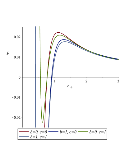
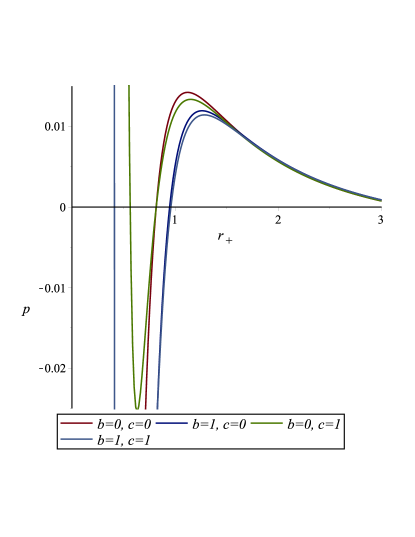
Figure 1: The plot of pressure for RN-AdS BH with GM for $\alpha=0.075$, $Q=0.85$ and $\Lambda=-0.1$ (left panel), $\Lambda=0.1$ (right panel).

In Fig. 1, we discuss the behavior of pressure for negative and positive values of cosmological constant. In both panels, we observe that the pressure decreases due to correction terms. For $b=1,c=1$, we observe the lowest trajectory of pressure then above it we have the trajectory of pressure at $b=1,c=0$ which becomes the logarithmic correction term. Furthermore, we see that the pressure increases for $b=0,c=1$ which is the second order correction term. The pressure is maximum if we avoid these correction terms. Also, we observe in both panels that the pressure increases for negative cosmological constant. However, the pressure becomes zero at $r_{+}=3.3$ for positive value of $\Lambda$ and becomes negative for large horizon while remains positive for negative value of $\Lambda$. Hence, we can conclude that the pressure decreases due to higher order correction terms and positive values of $\Lambda$. BHs derived from general relativity coupled with matter fields with $P\leq 0$ are thermodynamically unstable.

3.1 Stability of RN-AdS BH with GM

Here, we shall discuss the thermodynamical stability of RN-AdS with GM for which we can define

$$E|_{r=r_{+}}=\int TdS.$$ (26)

In BH thermodynamics, an important measurable physical quantity is the heat capacity or thermal capacity. The heat capacity of the BH may be stable or unstable by observing its sign (positive or negative), respectively. There are two types of heat capacities corresponding to a system such as $C_{v}$ and $C_{p}$ which determine the specific heat with constant volume and pressure, respectively. $C_{v}$ can be defined as

$$C_{V}|_{r=r_{+}}=T\left(\frac{\partial S}{\partial T}\right)_{V}.$$ (27)

Eqs. (22) and (24) lead to

$$C_{V}|_{r=r_{+}} = -\frac{2}{\pi r_{+}^{2}(r_{+}^{4}\Lambda+2\alpha r_{+}^{2}-3Q^{2}+r_{+}^{2})}\Big{(}-\pi^{2}r_{+}^{8}\Lambda+2\pi^{2}\alpha r_{+}^{6}+\pi br_{+}^{6}\Lambda$$ (28)

$$- \pi^{2}Q^{2}r_{+}^{4}+\pi^{2}r^{6}-\pi bQ^{2}r_{+}^{2}+cr_{+}^{4}\Lambda-2\alpha cr_{+}^{2}+cQ^{2}-cr_{+}^{2}\Big{)}.$$

Moreover, the $C_{p}$ can be evaluated as

$$C_{P}|_{r=r_{+}}=\left(\frac{\partial(E+PV)}{\partial T}\right)_{P},$$ (29)

and its expression can be obtained with the help of Eqs. (20), (22), (25) and (26) as

$$C_{P}|_{r=r_{+}} = -\frac{4}{\pi r_{+}^{2}(r_{+}^{4}\Lambda+2\alpha r_{+}^{2}-3Q^{2}+r_{+}^{2})}\Big{(}-3\pi^{2}r_{+}^{8}\Lambda+4\pi^{2}\alpha r_{+}^{6}$$ (30)

$$+ 2\pi br_{+}^{6}\Lambda-\pi^{2}Q^{2}r_{+}^{4}+2\pi^{2}r_{+}^{6}-cr_{+}^{4}\Lambda-cQ^{2}\Big{)}.$$

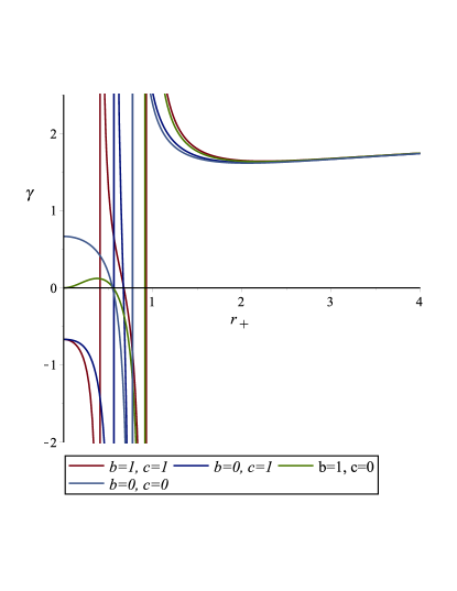
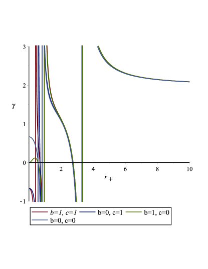
Figure 2: The plot of $\gamma$ versus horizon radius for RN-AdS BH with GM for $\alpha=0.075$, $Q=0.85$ and $\Lambda=-0.1$ (left panel), $\Lambda=0.1$ (right panel).

The above two specific heat relations can be comprises into a ratio that is denoted by $\gamma=C_{p}/C_{v}$ and its plot is given in Fig. 2. It can be noted that the value of $\gamma$ increases due to the correction terms. We find maximum value of $\gamma$ as $\gamma\rightarrow 2.1$ for positive value of $\Lambda$ and larger horizon, while for negative value of cosmological constant $\gamma\rightarrow 1.8$. Thus, one can observe that $\gamma$ exhibits more stable behavior for lower value of $\Lambda$ as compare to positive value of $\Lambda$. In left panel of Fig. 2, we observe that the value of $\gamma$ becomes higher by utilizing both correction and logarithmic correction terms in small horizon. Hence, it is pointed out that the value of $\gamma$ becomes higher due to correction terms and exhibits more stable behavior for lower values of $\Lambda$.

3.2 Phase transition

The stability of BH can be analyzed through $C_{v}$ (Eq. (28)) because $C_{v}\lesseqgtr 0$ corresponds to local stability of BH, phase transition and local instability of the BH.

$\Lambda$	correction terms	range of local stability	phase transition
$-0.1$	$b=1$, $c=1$ $b=0$, $c=1$ $b=1$, $c=0$ $b=0$, $c=0$	$0<r_{+}<0.4,0.92<r_{+}<1.53,r_{+}>3$ $0<r_{+}<0.55,0.76<r_{+}<1.53,~{}r_{+}>3$ $0.91<r_{+}<1.53,~{}r_{+}>3$ $0.77<r_{+}<1.53,~{}r_{+}>3$	$0.41,~{}0.93$ $0.56,~{}0.77$ $0.91$ $0.77$
0.1	$b=1$, $c=1$ $b=0$, $c=1$ $b=1$, $c=0$ $b=0$, $c=0$	$0<r_{+}<0.41,~{}0.95<r_{+}<1.27,~{}r_{+}>3.34$ $0<r_{+}<0.56,~{}0.81<r_{+}<1.27,~{}r_{+}>3.29$ $0.95<r_{+}<1.27,~{}r_{+}>3.34$ $0.81<r_{+}<1.27,~{}r_{+}>3.33$	$0.41,~{}0.96,~{}3.34$ $0.56,~{}0.82,~{}3.29$ $0.95,~{}3.34$ $0.82,~{}3.29$

Table 1: Range of local stability and critical points of horizon radius of phase transition for RN-AdS BH with GM due to the effect of higher order correction entropy.

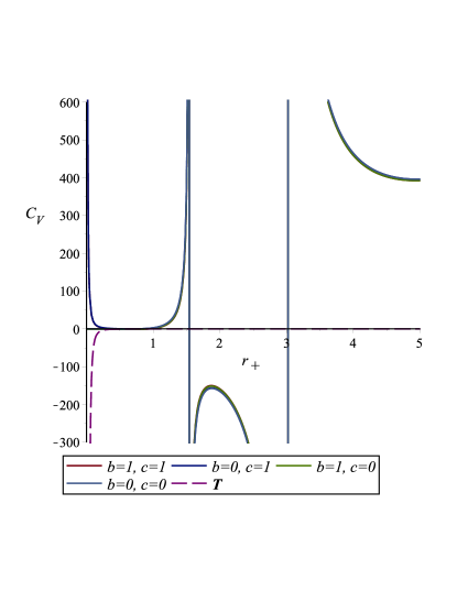
Figure 3: The plot of specific heat at constant volume for RN-AdS BH with GM for $\alpha=0.075$, $Q=0.85$ and $\Lambda=-0.1$ (left panel), $\Lambda=0.1$ (right panel)

We find the range of BH horizon of locally thermodynamical stability due to thermal fluctuations for negative and positive values of cosmological constant in left and right panels of Fig. 3, respectively and in Table 1. We can observe from Table 1 that the range of local stability is maximum for second order correction terms ($b=0,c=1$) as well as for both correction terms ($b=1,c=1$) as compare to the others in both cases of $\Lambda$. Moreover, we obtain the phase transition points for both case in Table 1. We observe that one can obtain more phase transition points for $b=0,c=1$ and $b=1,c=1$ as compare to others in both cases. Also, we find more phase transition points for positive value of cosmological constant as compare to negative value. It is noted that RN-AdS BH with GM is the most locally stable by considering the both correction terms for negative cosmological constant. We also find the different horizon regions where the BH is stable. For instance, it is completely stable for $r_{+}>3$ in the case of negative $\Lambda$ while for positive $\Lambda$, it is completely stable for $r_{+}\geq 3$. Hence, it can be concluded that if we increases the value of $\Lambda$ and consider the second order or both correction terms then we can find more phase transition points and the range of local stability is also increased.

3.3 Grand Canonical Ensemble

The BH can be considered as a thermodynamical object by treating it as grand canonical ensemble system where fix chemical charge is represented by $\mu=\frac{Q}{r_{+}}$. The temperature increases due to effect of chemical potential. The grand canonical ensemble is also known as Gibb’s free energy, which can be defined as

$$G=M-TS-\mu Q,$$ (31)

and it turns out to be

$$G|_{r=r_{+}} = -\frac{-r_{+}^{4}\Lambda+(2\alpha+1)r_{+}^{2}-Q^{2}}{8\pi^{2}r_{+}^{5}}\Big{(}-2\pi^{2}r_{+}^{4}-2c$$ (32)

$$+ b\ln\big{(}\frac{(-r_{+}^{4}\Lambda+2\alpha r_{+}^{2}-Q^{2}+r_{+}^{2})^{2}}{16\pi r_{+}^{4}}\big{)}\Big{)}-\mu r_{+}.$$

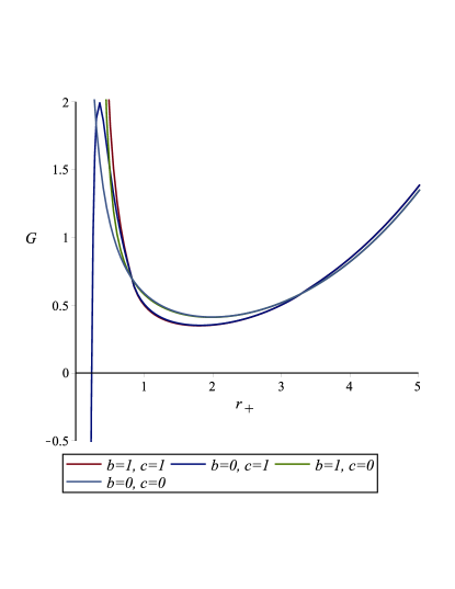
Figure 4: The plot of Gibb’s free energy for RN-AdS BH with GM for $\alpha=0.075$, $Q=0.85$ and $\Lambda=-0.1$ (left panel), $\Lambda=0.1$ (right panel)

Fig. 4 indicates the view of Gibb’s free energy for negative and positive cosmological constant. It can be noted from both panels of this figure that the correction terms reduce the Gibb’s free energy. In left panel, we observe that the BH is most stable for higher order correction terms ($b=1,c=1$ and $b=0,c=1$) near the singularity while it exhibits the most stable behavior at $r_{+}>0.8$ for second order correction term ($b=0,c=1$). In right panel, it is noticed that the BH is most stable for both correction terms ($b=1,c=1$) in the case for positive cosmological constant. Hence, it is concluded that RN-AdS with GM is the most stable BH for positive cosmological constant and higher order correction terms.

3.4 Canonical Ensemble

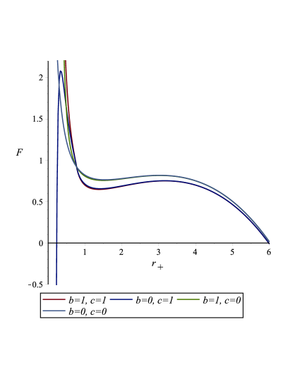
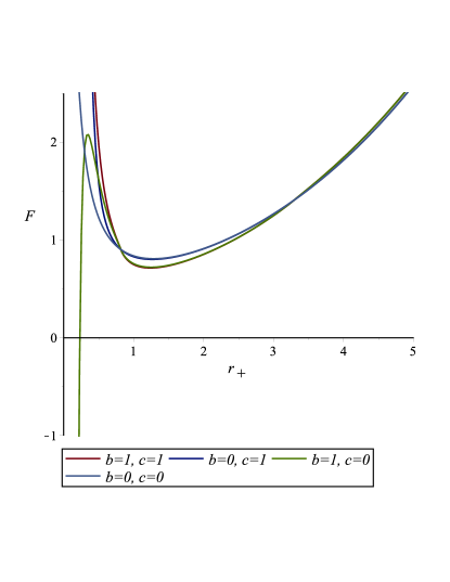
Figure 5: The plot of Helmhotz free energy versus horizon radius for RN-AdS BH with GM for $\alpha=0.075$, $Q=0.85$ and $\Lambda=-0.1$ (left panel), $\Lambda=0.1$ (right panel.

Here, we consider BH as a canonical ensemble (closed system) where transformation of charge is prohibited. For fixed charge, the free energy in canonical ensemble form termed as Helmhotz free energy and can be defined as

$$F=M-TS,$$ (33)

which becomes

$$F|_{r=r_{+}} = -\Big{(}-2\pi^{2}r_{+}^{4}-2c+b\ln\big{(}\frac{(-r_{+}^{4}\Lambda+2\alpha r_{+}^{2}-Q^{2}+r_{+}^{2})^{2}}{16\pi r_{+}^{4}}\big{)}\Big{)}$$ (34)

$$\times \frac{-r_{+}^{4}\Lambda+(2\alpha+1)r_{+}^{2}-Q^{2}}{8\pi^{2}r_{+}^{5}}.$$

The behavior of Helmhotz free energy for negative and positive cosmological constant is plotted in Fig. 5. In both panels, we observe that Helmhotz free energy decreases due to correction terms. For negative value of $\Lambda$, the BH is most stable for both correction terms ($b=1,c=1$) near the singularity while at $r_{+}>0.8$, it is the most stable for second order correction ($b=0,c=1$). For positive value of $\Lambda$, BH exhibits the most stable behavior for both correction terms at $r_{+}<0.8$ and $r_{+}>3.4$ while it is the most stable for second order correction term for $0.8<r_{+}<3.4$ approximately.

4 Thermodynamical Analysis of $f(R)$ BH

We consider the spherical symmetric metric of $f(R)$ BH of the form [38]

$$ds^{2}=f(r)dt^{2}-(f(r))^{-1}dr^{2}-r^{2}({d\theta}^{2}+\sin\theta{d\phi}^{2}),$$ (35)

where

$$f(r)=1+\frac{2M}{r}+\beta r-\frac{\Lambda r^{2}}{3}.$$ (36)

Here, $M$ is the mass of the BH, $\beta=a/d\geq 0$ is a constant with $d$ is the scale factor and $a$ is the dimensionless parameter [38]. The horizon radius can be obtained through metric function (36) as

$$r_{+}^{3}\Lambda--3r_{+}^{2}\beta+6M-3r_{+}=0.$$ (37)

One can obtain the mass and temperature of $f(R)$ BH at horizon radius as

$$M|_{r=r_{+}}=\frac{-r_{+}^{3}\Lambda+3\beta r_{+}^{2}+3r_{+}}{6},T|_{r=r_{+}} = \frac{-2r_{+}^{3}\Lambda+3\beta r_{+}^{2}+6M}{12\pi r_{+}^{2}}.$$ (38)

By utilizing the mass $M$ in above equation, the temperature reduces to

$$T|_{r=r_{+}}=\frac{-r_{+}^{2}\Lambda+2r_{+}\beta+1}{4\pi r_{+}}.$$ (39)

For real and positivity of temperature, we have

$$r_{+}\geq\frac{\beta+\sqrt{\beta^{2}+\Lambda}}{\Lambda}.$$ (40)

The condition satisfied

$$\beta^{2}+\Lambda\geq 0.$$ (41)

Since, the temperature is decreasing function of horizon radius, so when the size of black hole decreased, the temperature grow up and thermal fluctuations will be important. The higher order corrected entropy and pressure for this BH take the form

$$S|_{r=r_{+}} = \pi r_{+}^{2}-\frac{b}{2}\ln(\frac{(r_{+}^{2}\Lambda-2\beta r_{+}-1)^{2}}{16\pi})+\frac{c}{\pi r_{+}^{2}},$$ (42)

$$P|_{r=r_{+}} = \frac{1}{8\pi^{3}r_{+}^{6}}\big{(}-\pi^{2}r_{+}^{6}\Lambda+2\pi^{2}r_{+}^{5}\beta+b\pi r_{+}^{4}\Lambda-b\pi r_{+}^{3}\beta+\pi^{2}r_{+}^{4}+cr_{+}^{2}\Lambda$$ (43)

$$- 2cr_{+}\beta-c\big{)}.$$

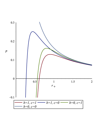
Figure 6: The plot of pressure for $f(R)$ BH for $\beta=1.5$ and $\Lambda=-0.1$ (left panel), $\Lambda=0.1$ (right panel)

In Fig. 6, we analyze the trajectories of pressure for negative and positive values of $\Lambda$. We can see pressure decreases due to correction terms. We obtain highest pressure in the absence of correction terms and the lowest pressure in the presence of both correction terms $(b=1,c=1)$. Also, we observe that the pressure is lower for second order correction term $(b=0,c=1)$ as compare to logarithmic correction term $(b=1,c=0)$. Interestingly, we find no change in pressure with respect to cosmological constant. Hence, it can be concluded that the pressure decreases due to higher order correction terms only.

4.1 Stability of $f(R)$ BH

For stability of $f(R)$ BH, we can obtain $C_{v}$ by using Eqs. (39) and (42) as follows

$$C_{V}|_{r=r_{+}} = -\frac{2}{\pi r_{+}^{2}(r_{+}^{2}\Lambda+1)}\Big{(}-\pi^{2}r_{+}^{6}\Lambda+2\pi^{2}\beta r_{+}^{5}+\pi br_{+}^{4}\Lambda$$ (44)

$$- \pi r_{+}^{3}\beta+\pi^{2}r_{+}^{4}+cr_{+}^{2}\Lambda-2\beta cr_{+}-c\Big{)}.$$

Moreover, $C_{p}$ can be obtained by using Eqs. (20), (39) and (43), we have

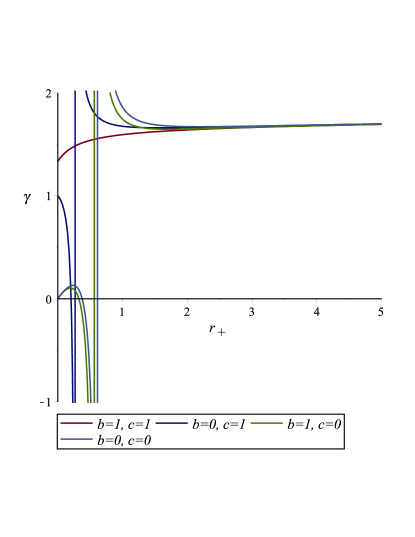
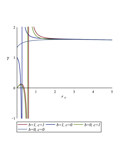
Figure 7: The plot of $\gamma$ for $f(R)$ BH for $\beta=1.5$ and $\Lambda=-0.1$ (left panel), $\Lambda=0.1$ (right panel)

$$C_{P}|_{r=r_{+}} = -\frac{2}{3\pi r_{+}(r_{+}^{2}\Lambda+1)}\Big{(}-6\pi^{2}r_{+}^{5}\Lambda+10\pi^{2}\beta r_{+}^{4}$$ (45)

$$+ 4\pi br_{+}^{3}\Lambda-3\pi b\beta r_{+}^{2}+4\pi^{2}r_{+}^{3}+2cr_{+}\Lambda-2c\beta\Big{)}.$$

For this BH, the plot of $\gamma=C_{p}/C_{v}$ is shown in Fig. 7. We observe that the value of $\gamma$ increases for larger horizon due to correction terms. Also, we find that the value of $\gamma$ is same for both cases (positive and negative values of $\Lambda$), i.e., $\gamma\rightarrow 0.6$ for larger horizon. Thus, we can say that $\gamma$ shows similar stable behavior for both cases of cosmological constant. It is realized that the value of $\gamma$ becomes higher due to correction terms and exhibits similar stable behavior for both cases of $\Lambda$ in $f(R)$ BHs.

4.2 Phase transition

$\Lambda$	correction terms	range of local stability	phase transition
$-0.1$	$b=1$, $c=1$ $b=0$, $c=1$ $b=1$, $c=0$ $b=0$, $c=0$	$0<r_{+}<0.61,~{}r_{+}>3.2$ $0<r_{+}<0.27,~{}r_{+}>3.2$ $0<r_{+}<0.56,~{}r_{+}>3.2$ $r_{+}>3.2$	$0.61$ $0.27$ $0.56$ $\phi$
0.1	$b=1$, $c=1$ $b=0$, $c=1$ $b=1$, $c=0$ $b=0$, $c=0$	$0<r_{+}<0.61,~{}r_{+}>30.33$ $0<r_{+}<0.26,~{}r_{+}>30.33$ $0<r_{+}<0.56,~{}r_{+}>30.33$ $~{}r_{+}>30.33$	$0.61,~{}30.33$ $0.26,~{}30.33$ $0.56,~{}30.33$ $30.33$

Table 2: Range of local stability and critical points of horizon radius of phase transition for f(R) BH due to the effect of higher order correction entropy

.

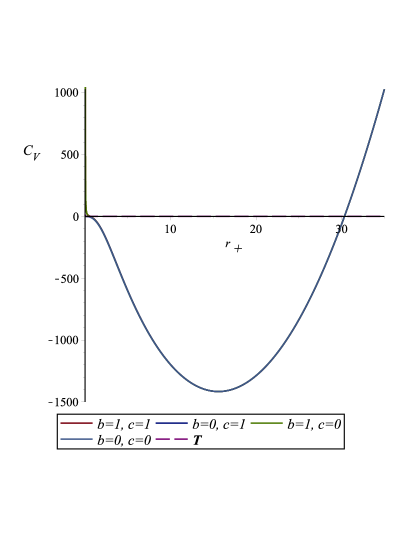
Figure 8: The plot of specific heat at constant volume for $f(R)$ BH for $\beta=1.5$ and $\Lambda=-0.1$ (left panel), $\Lambda=0.1$ (right panel)

We discuss the phase transition and range of local stability of BH horizon due to thermal fluctuation for negative and positive values of $\Lambda$. In both panels of Fig. 8, it is observed that the range of local stability is maximum for both correction terms and then the range of local stability is higher for second order correction term as compare to first order logarithmic correction term. Furthermore, we also find the phase transition points for both cases in Table 2. We obtain more phase transition points in the presence of correction term as compare to its absence. Moreover, we have more phase transition points for positive cosmological constant as compare to negative. We also observe that $f(R)$ BH is the most locally stable for $r_{+}>3.2$ in the case of negative $\Lambda$ while it is completely stable for $r_{+}>30.33$ in the case of positive $\Lambda$. Hence, we can conclude that if we utilize the correction terms and increases the value of cosmological constant then the range of local stability increases and we can obtain more phase transition points.

4.3 Grand Canonical Ensemble

The free energy in grand canonical ensemble (Gibb’s free energy) is given by

$$G|_{r=r_{+}} = -\frac{1}{24\pi^{2}r_{+}^{3}}\Big{(}2r_{+}^{6}\pi^{2}\Lambda+6r_{+}^{4}\pi^{2}+6cr_{+}^{2}\Lambda-12cr_{+}\beta-6c$$ (46)

$$- 3br_{+}^{2}\pi(r_{+}^{2}\Lambda-2r_{+}\beta-1)\ln\big{(}\frac{(-r_{+}^{2}\Lambda+2\beta r_{+}-1)^{2}}{16\pi}\big{)}\Big{)}-\mu r_{+}.$$

Figure 9: The plot of Gibb’s free energy for $f(R)$ BH for $\beta=1.5$ and $\Lambda=-0.1$ (left panel), $\Lambda=0.1$ (right panel)

Fig. 9 represents the behavior of Gibb’s free energy for negative and positive cosmological constant. In both panels, it is observed that the correction terms reduce the Gibb’s free energy. In left panel, we notice that the f(R) BH is stable for both correction terms ($b=1,c=1$) as compare to others while at $r_{+}=1$, we find the most stable BH by utilizing the logarithmic correction term ($b=1,c=0$). From right panel, we can see that Gibb’s free energy is higher for both correction terms and logarithmic correction term as compare to others. Hence, we can conclude that $f(R)$ BH is the most thermodynamically stable for higher order correction terms and positive cosmological constant.

4.4 Canonical Ensemble

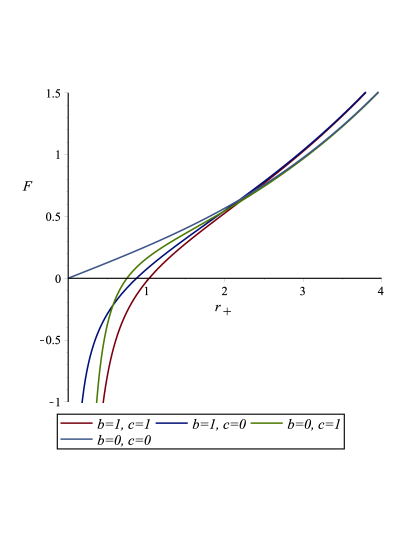
Figure 10: The plot of Helmhotz free energy for $f(R)$ BH for $\beta=1.5$ and $\Lambda=-0.1$ (left panel), $\Lambda=0.1$ (right panel)

The free energy in canonical ensemble is known as Helmhotz free energy if the charge is fixed, which is

$$F|_{r=r_{+}} = -\frac{1}{24\pi^{2}r_{+}^{3}}\Big{(}2r_{+}^{6}\pi^{2}\Lambda+6r_{+}^{4}\pi^{2}+6cr_{+}^{2}\Lambda-12cr_{+}\beta-6c$$ (47)

$$- 3br_{+}^{2}\pi(r_{+}^{2}\Lambda-2r_{+}\beta-1)\ln\big{(}\frac{(-r_{+}^{2}\Lambda+2\beta r_{+}-1)^{2}}{16\pi}\big{)}\Big{)}$$

The behavior of Helmhotz free energy for negative and positive cosmological constant is plotted in Fig. 10. In both panels, we observe that free energy decreases due to correction terms. In left panel, one can see the free energy is positive till $r_{+}=6$ and the BH is most stable for both correction term (red line) and second order correction term (green line) in the case of negative cosmological constant. In right panel, for positive value of $\Lambda$, BH is most stable for both correction term (red line) and logarithmic correction term (blue line) as compare to others. Hence, we can conclude that $f(R)$ BH shows most stable behavior for positive values of cosmological constant and higher order correction terms.

5 Conclusion

In this paper, we considered the RN-AdS BH with GM and $f(R)$ BH, and discussed the thermodynamics in the presence of higher order corrections of entropy. We utilize the results of corrected entropy by setting first order term is logarithmic and second order term is inversely proportional to original entropy. In these scenarios, we have studied the behavior of pressure and specific heat for both BHs. It is observed that the pressure reduces for second order correction term for both BHs but the pressure of RN-AdS BH with GM also decreases by considering higher values of cosmological constant while there is no change in pressure with respect to cosmological constant in $f(R)$ BH. We have also discussed the ratio of specific heat ($\gamma$) at constant pressure and volume for both BHs. We have observed that the value of $\gamma$ increases due to the effect of higher order correction terms for both BHs. The value of $\gamma$ for RN-AdS BH with GM exhibits more stable behavior for lower values of cosmological constant while $f(R)$ BH shows similar behavior for both (negative and positive) cases of $\Lambda$.

We have also studied the phase transition due to the effect of higher order correction terms for both BHs and obtained the phase transition points. We have noticed that the range of local stability and the phase transition points increases due to the effect of second order correction term and the higher values of cosmological constant for both BHs. We have investigated the free energy in canonical (Helmhotz free energy) and and grand canonical (Gibb’s free energy) ensembles. We have observed that the free energy reduces due to higher order correction terms. The Helmhotz free energy and Gibb’s free energy show the most stable behavior for both BHs in case of positive cosmological constant as compare to negative cosmological constant. We noticed that the both free energies exhibit the most stable behavior by utilizing the both correction terms ($b=1,c=1$). The Gibb’s free energy is reduced in both BHs due to chemical potential as compare to Helmhotz free energy. We also observe that both BHs exhibit the most locally stable behavior for negative cosmological constant while both BHs show the most globally stable behavior for positive values of cosmological constant. Hence, it is concluded that both BHs show the most locally stable behavior for second order correction term ($b=0,c=1$) while both BHs is most globally stable by utilizing the both correction terms ($b=1,c=1$), so it is better to consider the higher order correction terms.

References

- [1] J. D. Bekenstein, Phys. Rev. D, 7, 2333, (1973).
- [2] S. W. Hawking, Nature, 248, 30, (1974).
- [3] J. D. Bekenstein, Phys. Rev. Lett., 28, 452, (1972); J. D. Bekenstein, Phys. Rev. D, 5, 1239, (1972).
- [4] S. S. More, Clas. Quantum Grav., 22, 4129, (2005).
- [5] S. K. Rama, Phys. Lett. B, 457, 268, (1999).
- [6] A. Ashtekar, Lectures on Non-perturbative Canonical Gravity, World Scientific, (1991).
- [7] Govindarajan et al., Class. Quant. Grav., 18, 2877, (2001).
- [8] S. Das, P. Majumdar, R. Bhaduri, Class. Quantum Grav., 19, 2355, (2002).
- [9] A. Chatterjee, P. Majumdar, Phys. Rev. Lett., 92, 141301, (2004).
- [10] B. Pourhassan, S. Upadhyay, H. Farahani, Gen. Relativ. Gravit., 49, 144, (2017).
- [11] S. Carlip, Class. Quant. Grav., 17, 4175, (2000).
- [12] D. Birmingham, S. Sen, Phys. Rev. D, 63, 47501, (2001).
- [13] B. Pourhassan et al., Eur. Phys. J. C, 76, 145, (2016).
- [14] A. Jawad, M. U. Shahzad, Eur. Phys. J. C, 77, 349, (2017).
- [15] S. Perlmutter et al., Supernova Cosmology Project Collaboration. Astrophys. J., 517, 565, (1999).
- [16] D.N. Spergel et al., WMAP Collaboration. Astrophys. J. Suppl., 170, 377, (2007).
- [17] D. J. Eisenstein et al., SDSS Collaboration. Astrophys. J., 633, 560, (2005).
- [18] A. G. Riess et al., Supernova Search Team Collaboration. Astron. J., 116, 1009, (1998).
- [19] A. Ashtekar, Rep. Prog. Phys., 80, 102901, (2017).
- [20] A. Ahmed, U. Camci, M. Jamil, Class. Quant. Grav., 33, 215012, (2016).
- [21] M. Barriola, A. Vilenkin, Phys. Rev. Lett., 63, 341, (1989).
- [22] A. K. Bronnikov, B. E. Meierovich, E. R. Podolyak, J. Exp. and Theor. Phys., 95, 392, (2002).
- [23] H. Yu, Phys. Rev. D, 65, 087502, (2002).
- [24] J. Man, H. Cheng, Phys. Rev. D, 87, 044002, (2013).
- [25] A. A. Starobinsky, Phys. Lett. B, 91, 99, (1980).
- [26] N. Ohta, R. Percacci, G. P. Vacca, Phys. Rev. D, 92, 061501, (2015).
- [27] S. Soroushfar, R. Saffari, J. Kunz, C. Lammerzahl, Phys. Rev. D, 92, 044010, (2015).
- [28] M. U. Farooq, M. Jamil, D. Momeni, R. Myrzakulov, Can. J. Phys. 91, 703, (2013).
- [29] S. H. Hendi, Phys. Lett. B, 690, 220, (2010).
- [30] B. Majeed, M. Jamil, INT. J. MOD. PHYS. D, 26, 1741017, (2017).
- [31] B. P. Dolan, Class. Quantum Gravity, 28, 235017, (2011).
- [32] S. Hawking, D. N. Page, Commun. Math. Phys., 87, 577, (1983).
- [33] G. W. Gibbons, S. W. Hawking, M. J. Perry, Nucl. Phys. B, 138, 141, (1978).
- [34] R. F. Sobreiro, V. J. V. Otoya, Class. Quant. Grav., 24, 4937, (2007).
- [35] L. Bonora, A. A. Bytsenko, Nucl. Phys. B, 852, 508, (2011).
- [36] G. W. Gibbons, S. W. Hawking, Phys. Rev. D, 15, 2752, (1977).
- [37] V. Iyer, R. M. Wald, Phys. Rev. D, 52, 4430, (1995).
- [38] R. Saffari, S. Rahvar, Phys. Rev. D, 77, 104028, (2008).