Accurate, Data-Efficient Learning from Noisy, Choice-Based Labels for Inherent Risk Scoring

Abstract

Inherent risk scoring is an important function in anti-money laundering, used for determining the riskiness of an individual during onboarding before fraudulent transactions occur. It is, however, often fraught with two challenges: (1) inconsistent notions of what constitutes as high or low risk by experts and (2) the lack of labeled data. This paper explores a new paradigm of data labeling and data collection to tackle these issues. The data labeling is choice-based; the expert does not provide an absolute risk score but merely chooses the most/least risky example out of a small choice set, which reduces inconsistency because experts make only relative judgments of risk. The data collection is synthetic; examples are crafted using optimal experimental design methods, obviating the need for real data which is often difficult to obtain due to regulatory concerns. We present the methodology of an end-to-end inherent risk scoring algorithm that we built for a large financial institution. The system was trained on a small set of synthetic data (188 examples, 24 features) whose labels are obtained via the choice-based paradigm using an efficient number of expert labelers. The system achieves 89% accuracy on a test set of 52 examples, with an area under the ROC curve of 93%.

1 Introduction

Financial institutions today are tasked with Know Your Customer obligations in order to mitigate money laundering activity in their systems that often serves to enable terrorism or drug trafficking. Banks as a result have collected large amounts of background information about their customers, such as their source of funds, business operations, and financial statements. Accurately predicting customer inherent risk from this information is a critical function in preventing money laundering and other fraudulent behaviors before they happen.

Despite the abundance of customer information (features), there is a paucity of data on actual instances of financial crime (labels). Traditionally, expert money laundering investigators are employed to sift through large amounts of customer records and provide their judgments on (i.e., act as a prediction module for) the risk level of each individual. Because such a process is costly, manual, and time-consuming, much work is focused on building accurate machine learning models for predicting inherent risk.

Inherent risk is a concept that most find easy to evaluate in comparisons. For example, one might easily judge that a politically exposed person with frequent transactions of more than $10k to foreign parties is inherently riskier compared to a customer with smaller, more stable transactions, who in turn is inherently riskier compared to a long-established domestic customer on a fixed-term deposit. However, due to the subjective and ever-changing nature of the notion of risk, it is far more difficult to judge the inherent risk of an individual on a standard scale, e.g., between -1 and 1, than it is to make comparisons between different examples. In practice, investigators are often asked only to provide labels on a binary scale of either “high” or “low” risk. While such binning strategies may make it easier for investigators, they also allow for highly inconsistent and noisy labels, because different investigators have different ideas of what constitutes as, e.g., “high” risk.

1.1 Contributions

To address the noisy and subjective nature of inherent risk labeling, we present a novel method for obtaining standard scale continuous valued labels of inherent risk from purely choice-based queries from a crowd of expert labelers. Contributions include the following: (1) leveraging a Monte Carlo D-optimal design-of-experiments approach for generating a set of synthetic customer examples which covers the input space without bias; (2) an optimal algorithm for generating choice sets which minimizes redundant pairings; and (3) a formulation which aggregates choice-based queries into continuous target values with maximal, unbiased use of the information provided. Finally, we show that our end-to-end algorithm learned from such labels achieves a classification accuracy of 89% on a test set of customers. This is, to the authors’ knowledge, the first time choice-based conjoint analysis techniques have been successfully applied to financial crimes risk prediction.

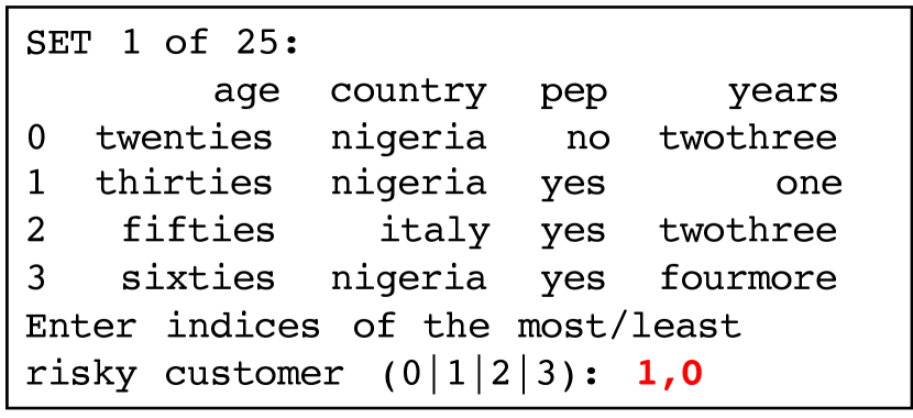
(a) Example of a choice set.

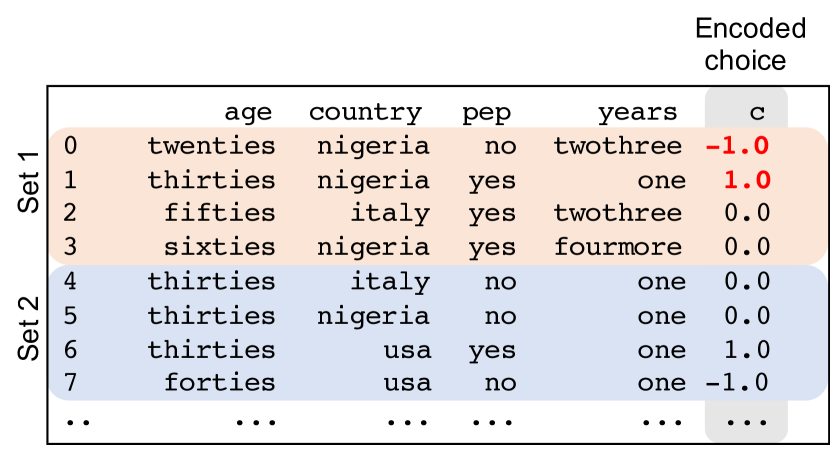
(b) Example data layout.

Figure 1: Illustration of the choice-based format for querying the experts. (a) Experts are presented with a small minibatch (choice set size of 4 here) of examples, and they are asked to select only the highest and lowest risk example from within that set. (b) Layout of the data obtained after labeling of a choice-based questionnaire. Most/least risky examples from each choice set are encoded as 1/-1 while unselected examples are encoded as 0. These encodings are mean-aggregated over multiple questionnaires (with different minibatching) to obtain the final label. See Section 2.3 for more discussion.

2 The Choice-Based Labeling Paradigm

2.1 Conjoint Analysis: A questionnaire of Label Querying Formats

We first motivate the need for choice-based label querying. Conjoint analysis is a method wherein the responses from one or more human labelers (who have access to the oracle labeling function with some error, i.e., $y=f(x)+\epsilon$) are used to label a set of examples for supervised training. The labels can be queried in several formats, including direct, ranking, or choice formats. Table 1 summarizes their properties.

The direct label format is typically assumed in most machine learning formulations (i.e., $y_{i}$ is directly queried for every example $x_{i}$). However, in risk scoring, the expert often has a relative notion of the true label and is unable to provide $y_{i}$ directly. Binning the label value into discrete ordinal values (e.g., high/medium/low) is one solution but still suffers from subjectivity.

In contrast, the ranking and choice formats demand less of the expert—they require only pairwise comparisons (e.g., Is example A riskier than example B?) which alleviate the need for labeling on a standard, absolute scale. Such labeling formats are often employed in marketing to learn customer preferences on variations of potential products, where again the expert, i.e., customer, has only a relative notion of the true label, i.e., utility of one product vs. another (Asioli et al. [2016]). Table 1 shows a comparison of the three formats.

The ranking format asks the expert to sort the entire set of examples according to their target value (risk score in our case), a task that can be broken down into a series of pairwise comparisons. However, it is time-consuming for a human expert to sort hundreds or thousands of examples—using MergeSort, one could achieve $O(n\log n)$ time complexity at best. In the choice format, the expert is presented with small choice sets, or minibatches, of examples and asked only to select the most and least risky examples from within that set. In addition to having a time complexity of $O(n)$, choice-based formats tend to be most natural for human experts (Sethuraman et al. [2005]) because human experts can “eye-ball” the choice set and quickly determine the examples at the extremes of the risky/non-risky spectrum, without needing to deliberate between the relative risk levels of those examples in between. For these reasons, the choice-based format is most popular in conjoint analysis and is the format that we will henceforth consider. Figure 1(a) shows an example of a choice set, and Figure 1(b) shows an example of how choice-based information queried from the human experts is stored.

Table 1: Comparison and descriptions of three formats of label querying.

Format	Information obtained	Mathematical expression
Direct	Continuous valued labels	$y_{i},\forall i$
Ranking	Ranking of all labels	$\{r(i),\forall i\mid y_{i}\!>\!y_{j},\forall\>r(i)\!>\!r(j)\}$
Choice	Max/min label w/in choice set	$\big{\{}\underset{j\in S_{k}}{\mathrm{argmax}}\ y^{j},\forall\ S_{k}\in Q\big{\}}\cup\big{\{}\underset{j\in S_{k}}{\mathrm{argmin}}\ y^{j},\forall\ S_{k}\in Q\big{\}}$

2.2 The Choice-Based Questionnaire

Suppose we have an unlabeled dataset of $n$ examples, $X=\{x_{1},\cdots,x_{n}\},x_{i}\in\mathcal{X}$, for which we wish to obtain absolute-scale, continuous-valued labels suitable for supervised training, i.e., $Y=\{y_{1},\cdots,y_{n}\},y_{i}\in\mathcal{Y}\subseteq\mathbb{R}$. In choice formats, the examples are partitioned in to $n/s$ choice sets (minibatches) each of size $s$. Experts are then asked to choose the most and least risky example within each choice set, $S_{k}=\{x^{k},\cdots,x^{k+s-1}\},x^{i}\in X$. The identifier function, $t:x^{t(i)}=x_{i}$, is assumed to be known. The superset of choice sets encompassing all $n$ examples is called the questionnaire, $Q=\{S_{1},\cdots,S_{n/s}\}$. There may be multiple questionnaires $Q_{1},\cdots,Q_{q}$ assigned to multiple experts; however, each questionnaire consists of the same set of examples $X$, and each example $x_{i}$ appears only once in each questionnaire. The partitioning (or minibatching) of choice sets should, however, be different across questionnaires to increase the diversity of pairwise comparisons (i.e., $Q_{i}\cap Q_{j}=\emptyset,\forall\ i\!\neq\!j$). A method for maximizing pairwise diversity is presented in Section 3.4. We allow the experts to have some zero-mean uncertainty $\epsilon$ in their judgment.

2.3 From Choice to Score

In the $l$-th questionnaire, we encode the choice $c$ of example $i$ as follows:

$$c(y_{i}|l)=\begin{dcases}1,&\text{if }y_{i}=\max_{j\in S_{k}}y^{j}\\ -1,&\text{if }y_{i}=\min_{j\in S_{k}}y^{j}\\ 0,&\text{otherwise}\end{dcases}$$ (1)

Here, $S_{k}$ is the choice set which hosts $x_{i}$ in questionnaire $l$. We then compute the mean choice $\bar{c}_{i}$ by averaging the choice $c(y_{i}|l)$ for example $i$ across all $q$ questionnaires:

$$\bar{c}_{i}(y_{i})=\frac{1}{q}\sum_{l=1}^{q}c(y_{i}|l)$$ (2)

We seek to know the functional relationship between mean choice and risk score so that we can convert the relative choice-based questionnaire results to a stand-alone, absolute-scale measure of risk, i.e., the label $y$, for supervised training. Given a label distribution $P(Y=y)=f(y)$ as a prior, the expected choice of example $i$ can be derived as:

$$\begin{split}\braket{c(y_{i})}&=\mathbb{E}_{y_{i}\sim Y}\enspace c(y_{i})\\ &=+1\times P(y_{i}\!=\!\max_{j\in S_{k}}y^{j})\\ &\quad-1\times P(y_{i}\!=\!\min_{j\in S_{k}}y^{j})\\ &\quad+0\times P(y_{i}\text{ is neither max nor min})\end{split}$$ (3)

Based on independence (i.e., examples are placed into choice sets without regard for the others selected), the probability that example $i$ has the largest true label within its choice set is:

$$\begin{split}P(y_{i}\!=\!\max_{j\in S_{k}}y^{j})&=\prod_{j\in S_{k},j\neq i}P(y_{i}\!>\!y^{j})\\ &=\prod_{j\in S_{k},j\neq i}\left(\int_{-\infty}^{y_{i}}f(y^{j})\>\mathrm{d}y^{j}\right)\\ &=\left(\int_{-\infty}^{y_{i}}f(y^{\prime})\>\mathrm{d}y^{\prime}\right)^{s-1}\end{split}$$ (4)

A similar derivation can be made for the probability that example $i$ has the smallest true label. Substituting that and Eq. 4 into Eq. 3, the relationship between the expected choice and risk score is:

$$\braket{c(y_{i})}=\left(\int_{-\infty}^{y_{i}}f(y^{\prime})\>\mathrm{d}y^{\prime}\right)^{s-1}-\left(\int_{y_{i}}^{\infty}f(y^{\prime})\>\mathrm{d}y^{\prime}\right)^{s-1}$$ (5)

There is no analytical inverse for Eq. 5, but the inverse is readily estimated by numerical optimization. In the limit of a large number of questionnaires, the mean choice (which is measured) and expected choice converge:

$$\lim_{q\to\infty}\bar{c}(y_{i})=\braket{c(y_{i})}$$ (6)

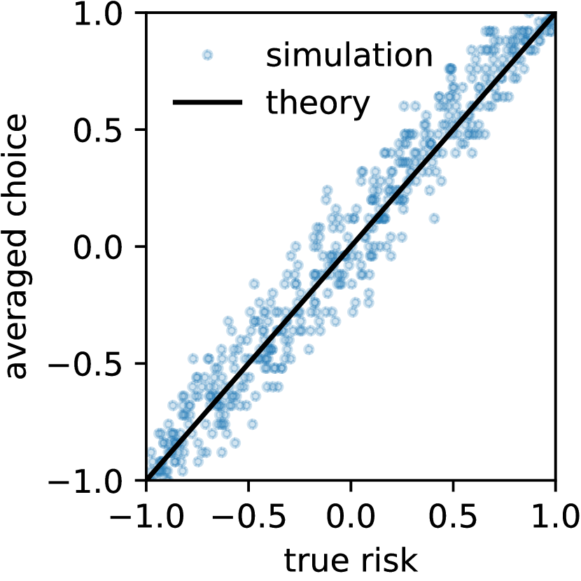
(a) Choice set size = 3

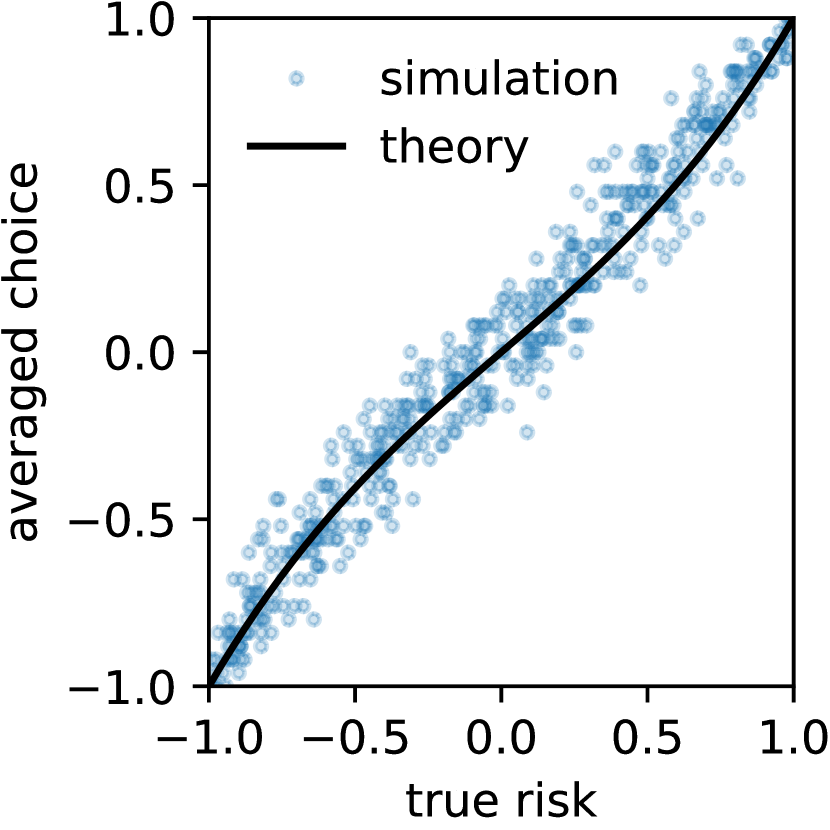
(b) Choice set size = 4

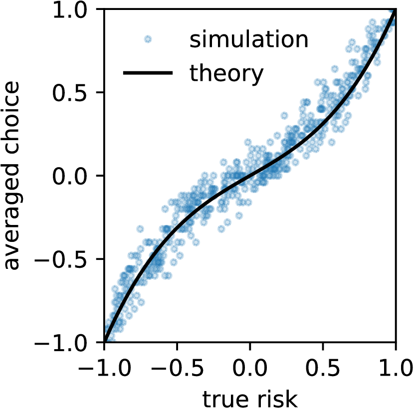
(c) Choice set size = 5

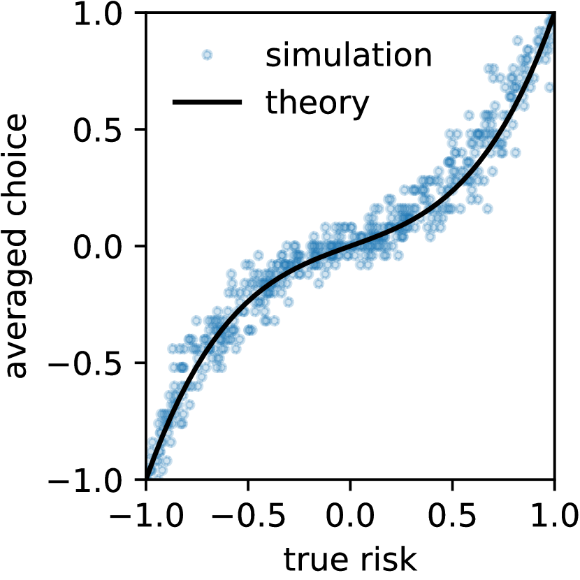
(d) Choice set size = 6

Figure 2: Simulation results showing averaged choice as a function of true label for 500 different examples (blue dots). An oracle evaluated each of the examples using the choice-based paradigm over 25 questionnaires. The examples’ true labels are sampled from a uniform distribution.

Example Consider a uniform label distribution $f(y)=1/2$ for $y\in[-1,1]$. The expected choice based on Eq. 5 is:

$$\braket{c(y_{i})}=\left(\frac{y_{i}}{2}+\frac{1}{2}\right)^{s-1}-\left(-\frac{y_{i}}{2}+\frac{1}{2}\right)^{s-1}$$ (7)

We conduct a simulation of 25 questionnaires each with the same set of 500 examples whose labels are sampled from a uniform distribution between -1 and 1. In each questionnaire, the examples are randomly partitioned into choice sets of size $s$. Within each choice set, an oracle is used to provide the choice $c_{i}$ for each example as to whether it is most/least/neither risky within its respective choice set. The choices are encoded and mean aggregated as described by Eqs. 2, 3. Figure 2 plots the averaged choice for each example as function of its true label. The simulation data fits our theoretical result perfectly, verifying that the choice-to-score relation in Eq. 5 can be used to convert relative information to absolute information about the labels.

3 End-to-End Algorithm for Inherent Risk Scoring

3.1 Overview

We now present the Inherent Risk Model (IRM) built for a large financial institution. The data consisted of all customers active over the course of a four-year period. All entities considered were banking participants during that time period. The IRM was developed with the intended purpose of being used as a risk prioritization framework to quickly estimate the probability that a given customer’s profile of Know Your Customer (KYC) variables was a high or low inherent risk for being involved in money laundering activity. The IRM’s prediction of a customer’s inherent risk based on KYC variables, without access to transaction information, was designed to mimic the kind of information that an anti-money laundering investigator, henceforth called Subject Matter Advisor (SMA), has access to when performing a first-level money laundering screening. Each customer (example) consisted of 24 variables (features), which included basic customer information, KYC risk flags, behavioral markers, and triggered alerts (we have redacted the specific variable names to protect the parties involved). Roughly 150,000 unique customer profiles were available.

3.2 Synthetic Examples via Optimal Experimental Design

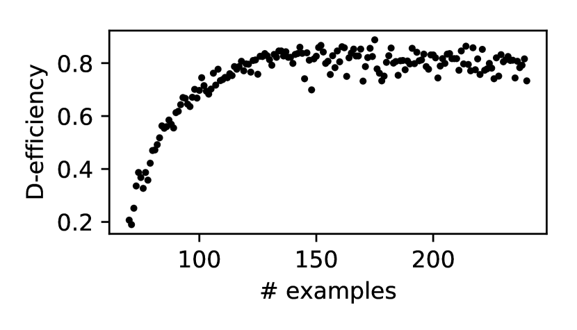
(a) Optimal D-efficiency computed by the optMonteCarlo function in R as a function of the number of examples. There are diminishing returns after about 120 examples.

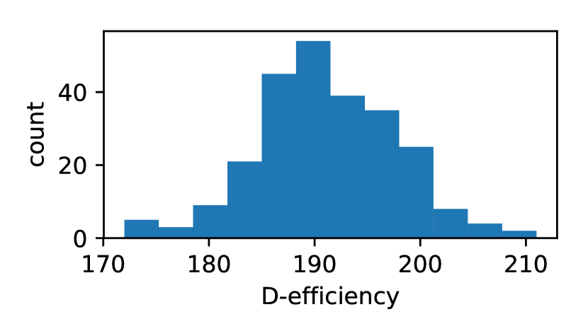
(b) Results of a simulation of 250 trials, for a fixed list of attributes and attribute levels, where the D-optimal number of profiles is returned from a sample size of 5 for one trial.

Figure 3: Results of our optimal experimental design using the optMonteCarlo package in R.

While we had access to many examples (i.e., customer profiles), we did not want our trained model to depend on the particular distribution of our training data, as distributions can vary across different institutions. Plus, we did not have the SMA resources to label such a large dataset. To eliminate these issues, we created a synthetic dataset of examples using Optimal Experimental Design (OED). OED operates under the assumption that obtaining a label for each example is costly and presents a theory for selecting examples that, given labels, predict the target variable as well as possible. In particular, we seek to optimize the D-efficiency, defined as $|X^{T}X|$ where $X\in\mathbb{R}^{n\times m}$ is the matrix of all $n$ examples with $m$ features. Maximizing D-efficiency makes the $n$ examples span the largest possible region in feature space, ensuring that the examples are as orthogonal and balanced as possible (Eriksson et al. [2000]).

Optimal experimental design is obtained for the model discussed in this letter through the use of the Federov Coordinate Exchange algorithm via Monte Carlo implemented in the optMonteCarlo function of the R library AlgDesign. Only linear terms were considered. We observe that the D-efficiency increases with the number of examples allowed up to about 120 examples, after which the gain in D-efficiency diminishes. See Figure 3(a). A simulation was then performed to assess stability of this result. optMonteCarlo was called on the collection of 24 business-approved features returning the maximum D-efficiency observed across a sample size of five, constituting one trial. Figure 3(b) shows 250 trials and identifies an optimal example count range from 185 to 190. An example count of 188 was selected based on the group theoretic results of Section 3.4.

3.3 Choice Set Size Selection

We now determine the optimal amount of information that we can obtain from the SMAs as a function of choice set size. We attack this problem using error analysis on simulations that we performed like the one in Section 2.3. 188 profiles are sampled from a normal label distribution, and we simulate the oracle responses to $q$ questionnaires to obtain the mean choice $\bar{c}_{i}$. The mean choice is then converted to an estimated label by Eq. 5. Next, we calculate the error per example as the difference between that example’s estimated label and its true label. We then take the RMS of the error across all the examples as a measure of how well the information from the SMAs approximates the ground truth. Figure 4(a) shows the RMS error as a function of the number of questionnaires and choice set size. It is apparent that a choice set size of 2 has the most RMS error; this makes sense because knowing the least risky example in a 2-example choice set is redundant when the most risky example is already known, so only one pairwise comparison’s worth of information is obtained. On the other hand, in choice set sizes of 3, at least 3 pairwise comparisons’ worth of information is obtained between the most risky, least risky, and in-between profiles. Choice set sizes of 3 and beyond have similar RMS errors, with set sizes 4 and 5 having the minimum values. Based on this analysis, we chose a choice set size of 4.

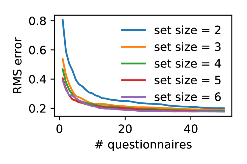
(a) RMS error between the true label and the label obtained by taking the inverse of Eq. 5 on a set of 188 examples. As the number of questionnaires increases, the error converges to zero. A choice set size of 4 yielded the lowest error at 20 questionnaires, informing our decision of using that size.

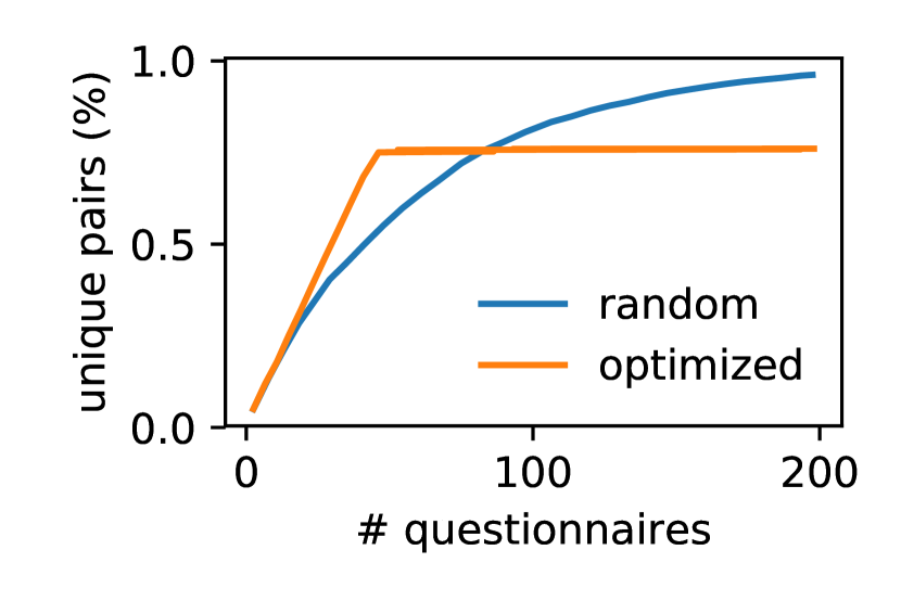
(b) Percentage of unique pairs within the choice sets of $q$ questionnaires, where $q$ is the x-axis. Random and optimized (group theoretic) choice sets are compared and demonstrated for 188 examples on 47 choice sets with prime number factors 13, 17, and 19.

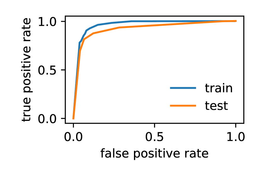
(c) Inherent Risk Model ROC curve on SMA-evaluated questionnaires. The champion model was logistic regression with a threshold for positive/negative classification. Area under the curve was 97% on train and 93% on test.

Figure 4: Results of (a) choice set size selection, (b) choice set optimization, and (c) ROC curve of model on train and test sets.

3.4 Choice Set (Minibatch) Optimization

Given $q$ questionnaires, how should examples be partitioned (minibatched) into choice sets to maximize the amount of information obtained? Since the base unit of relative information is the pairwise comparison, here we present a group theoretic method that maximizes the amount of unique intra-choice-set pairs as a proxy to maximizing the amount of information obtained through the questionnaires. We show in Figure 4(b) that our method achieves 75% of the possible unique pairwise comparison in half the number of questionnaires as compared to random minibatching.

Choice-based analysis references do not address information-theoretic concerns about the information extracted when the ground truth is not absolutely defined. The authors are not aware of a mechanism or technique that provides guidance on how to optimize the maximal information extracted from choice-based generated questionnaires. While optimal profiles were generated using the concept of D-optimality, the construction of the questionnaires itself is a combinatorics question handled by a computer if the problem size is small. Optimizing the arrangement of profile IDs is similar to the class of problems called backtracking. Randomly selecting the choice sets from over $10^{9}{\sim}185^{4}$ combinations and checking each against the required matching conditions that guarantee minimizing profile comparison redundancy, over a modest number of questionnaires, is not computationally tractable. We seek to develop a questionnaire generation optimization that uses each profile once per questionnaire and minimizes the redundant inferred choice set size two comparisons to approach an information-theoretic limit for information extraction. We achieve a general solution to this problem by constructing a reducible matrix representation of a finite group whose cycle corresponds to the maximum number of unique questionnaires that can be constructed given the representation.

We can motivate this approach by discussing the pairwise combinations of choice set profiles found in a choice set of size 4. The SMA’s act of observation is on one choice set at a time. The SMA assesses the relative risk of the profiles presented in that choice set, selecting one profile as highest relative risk and one profile as lowest relative risk. From one SMA’s evaluation of a choice set of size four, we can infer two of the four size three inferred choice set evaluations, and five of the six size two choice set evaluations. On four elements, five of the six pairs are implied. It is the opinion of the authors that this comparison of different choice sets sizes is similar to an analysis of reducible finite group representations as they are compositions of irreducible representations. We use this insight to generate a group theoretic questionnaire optimization of choice sets. The uniqueness of the result guarantees that any other sampling methodology obtaining this rate of unique pairs per questionnaire is isomorphic to the underlying group representation we construct. This also implies that no other algorithmic process can obtain a faster unique enumeration of pairs for a collection of choice sets.

We present this result as an application of the Polya Enumeration Theorem in Algorithm 1.

Algorithm 1 Choice Set Diversifier - Size 4

  Input: Range of D-optimal profiles $R$

  Select $c\in\mathbb{N}$ and $c\in R$ such that $c=4p$ where $p$ is prime; $p$ is the number of choice sets

  Select three different prime numbers $p_{1},p_{2},p_{3}$ such that $3<p_{i}$ and $p<p_{i}p_{j}$ for $i\neq j$.

  Without replacement, randomly Assign each of the $4p$ profiles a profile key from $1$ to $4p$ and place them into equal sized lists: $[A,B,C,D]$

  Construct a $rank(p)$ square identity matrix, $\mathbb{I}$

  For each prime number $p_{1},p_{2},p_{3}$: Construct a $rank(p)$ square permutation matrix, $\hat{G}_{p_{1}}$, $\hat{G}_{p_{2}}$, $\hat{G}_{p_{3}}$:Where elements of $[B,C,D]$ are mapped by position index $i$ in each list such that$i\mapsto i+p_{1}$ modulo $p$ OR $i\mapsto i+p_{2}$ modulo $p$ OR $i\mapsto i+p_{3}$ modulo $p$

  Define a Group Action $\hat{\textbf{G}}$ on the vector space of ordered tuples $\braket{a,b,c,d}$ where $a\in A,b\in B,c\in C,d\in D$ such that $\hat{G}=\mathbb{I}\oplus\hat{G}_{p_{1}}\oplus\hat{G}_{p_{2}}\oplus\hat{G}_{p_{3}}$ and $\hat{G}^{(p+1)}=\hat{G}$

  Action on a Choice Set is given by $\hat{G}(\braket{a_{1},b_{1},c_{1},d_{1}})=\mathbb{I}*a_{1}\oplus\hat{G}_{p_{1}}*b_{1}\oplus\hat{G}_{p_{2}}*c_{1}\oplus\hat{G}_{p_{3}}*d_{1}=\braket{a_{1},b_{1+p_{1}},c_{1+p_{2}},d_{1+p_{3}}}$

  Append each ordered list $[A,B,C,D]$ so that $U=A+B+C+D$. $U$ is the first questionnaire

  Apply $\hat{\textbf{G}}$ to the randomized ordered list $U$ to generate the next questionnaire

  Stop when $\hat{G}$ has been applied to $U$ $p$ number of times

  Return $p$ number of unique questionnaires $U$, $U^{\prime}$, $U^{\prime\prime}$, $\cdots$

We now have four permutation matrices (one is the identity matrix) that separately act on a choice set element. If the list of choice sets is a $4*p$ length row vector comprising one questionnaire, $\hat{G}$ becomes a $4*p$ dimensional representation with subsequent applications of $\hat{G}$ generating unique questionnaires until repeating on the $p+1$ questionnaire. This generates an optimal collection of questionnaires where each profile is used once per questionnaire, each choice set combination appears at most once for all questionnaires, and any two out of the four profiles in any choice set appear at most once over all questionnaires. This result motivated our choice of $n=188$ examples with prime number factors 13, 17, 19.

3.5 Training and Evaluation

Synthetic Data. Our inherent risk scoring model was trained, validated, and tested on the collected questionnaire results from a team of SMAs. The questionnaires consisted of unique choice sets of synthetic KYC profiles as per the complete methodology outlined in this paper. We trained a linear classifier on the 188 customer profiles from the training set. We separately obtained a test set of 52 examples from the same SMAs via the same approach. We define a threshold in the range of [-1,1] to separate profiles that are considered high (e.g., positive prediction) and low risk (e.g., negative prediction). The ROC curve as a function of this threshold is shown in Figure 4(c). We tuned the threshold to be compliant with an industry standard false-negative (misclassifying a high risk customer as low risk) rate of roughly 1:1,000. At this threshold, we achieved an area under the curve (AUC) of 97% on train and 93% on test, with a classification error of 8% on train and 11% on test.

Real-World Data. The same IRM model was applied to the customer population and provided a rank-ordering of those profiles. A logic layer stating the presence of 1 of 14 scenarios associated with risky trading, transaction, or settlement behavior conditioned the sample down to roughly 8,000 unique customers. The remaining alerted accounts were individually reviewed, providing a rare performance evaluation for the model on real-world data. The prioritization framework created with the authors’ complete methodology was tested by letting it select the 1,500 profiles it predicted to be the riskiest, partitioning the alerting population. After SMAs reviewed the 4,000 profiles and identified which ones should be recommended for escalation, the IRM capability to pick truly “riskier” profiles resulted in a 15.5x improvement in the escalation rate. Compared with the escalation rate associated with a random alerting profile of 0.775%, the IRM achieved a 2.4x improvement. None of the 31 SMA-recommended escalations were in the bottom 40% of the IRM risk score, highlighting a low false-negative rate.

Table 2: IRM performance on SMA-evaluated questionnaires.

Metric	Train	Test
AUC	97%	93%
Classification Error	8%	11%

Population Group	Profiles	SMA Escalations	Escalation Rate
IRM Selected Alerted Profiles	1,500	28	1.87
Remaining Scenario Alerted Profiles	2,500	3	0.12

4 Related work

Ratner et al. [2016] presented the idea of programmatically generating (possibly noisy) training data using distant supervision and rule-based labeling functions. The fact that noisy, crowdsourced training data may still be used to achieve high accuracy models forms the basis of our approach. Generating labels from alternative feedback (other than direct labels) is not new: much work has been done in the field of learning to rank via pairwise preferences (Hullermeier et al. [2008], Jamieson and Nowak [2011]). Xu et al. [2018] considers the leveraging of ranking or comparison information as a way to improve on their model, but their method assumes that some number of direct labels are known, whereas we do not make this assumption. Choice-based conjoint analysis has been widely used in preference learning (Asioli et al. [2016]) in marketing, but has not been applied to risk assessment.

5 Conclusion

We have introduced a novel end-to-end methodology for developing machine learning models trained on labels that are defined by relative comparisons in the absence of absolute label definitions. Our model, used for inherent risk prediction, was trained on a set of choice-based responses to group theoretic optimized questionnaires consisting of synthetic examples. The model was applied to real-world profiles to evaluate the money laundering risk of banking customers. We achieved a 15.5x improvement of the identification rate of customer profiles that money laundering experts recommended for escalation. Broadly, these results challenge the community to consider the class of machine learning problems where expert feedback is missing absolute label definitions and labels must be gathered from alternative feedback methods, such as choice.

Two shortcomings of our approach are listed here to stimulate further research. First, our formulation assumes oracle questionnaire respondents who choose the most/least risky customer in each choice set with no mistakes with regard to their ground truth risk score. In reality, human experts in this domain will have differing biases and noise in their responses. Second, we assume that the label distribution is known. While it is reasonable to assume a normal distribution, based on the central limit theorem, in the case of a linear model and D-optimal example set, this is a restrictive condition.

Acknowledgments

The people referenced in this acknowledgements section are the authors’ colleagues at Ernst & Young LLP, and we thank them for their support. The authors thank Jonathan DeGange and Carl Case for detailed preliminary technical conversations that seeded this work. Jonathan DeGange’s contributions as an expert in Monte Carlo methods were critical to this work. Nick Brennan, Zachary Carideo, and Maoxin Ye provided data science support and experimentation. Finally, the authors thank Ron Giammarco, Darrin Williams, Sameer Gupta, Carl Case, Ali Khan, Jonathan DeGange, Joe Kruse, Greg Capece, and Rajarajan Sampath for project oversight and support. The results discussed in this letter and references to terms accurate, efficient, and bias are with respect to the letter’s mathematical treatment of a generalized methodology framework. The views and conclusions expressed in this material are those of the authors and should not be interpreted as representing the official policies or endorsements, either expressed or implied, of Ernst & Young LLP.

References

- Asioli et al. [2016] D. Asioli, T. Nass, A. Avrum, and V.L. Almli. Comparison of rating-based and choice-based conjoint analysis models. a case study based on preferences for iced coffee in norway. Food Quality and Preference, 48:174 – 184, 2016. URL http://www.sciencedirect.com/science/article/pii/S0950329315002499.
- Sethuraman et al. [2005] Raj Sethuraman, Roger A Kerin, and William L Cron. A field study comparing online and offline data collection methods for identifying product attribute preferences using conjoint analysis. J. Bus. Res., 58(5):602–610, 2005. ISSN 0148-2963. doi: https://doi.org/10.1016/j.jbusres.2003.09.009. URL http://www.sciencedirect.com/science/article/pii/S0148296303002029.
- Eriksson et al. [2000] L. Eriksson, E. Johansson, N. Kettaneh-Wold, C. Wikstrom, and S. Wold. Design of Experiments: Principles and Applications. Learnways AB, 2000.
- Ratner et al. [2016] Alexander J Ratner, Christopher M De Sa, Sen Wu, Daniel Selsam, and Christopher Ré. Data programming: Creating large training sets, quickly. In Advances in Neural Information Processing Systems 29, pages 3567–3575. 2016. URL http://papers.nips.cc/paper/6523-data-programming-creating-large-training-sets-quickly.pdf.
- Hullermeier et al. [2008] Eyke Hullermeier, Johannes Farnkranz, Weiwei Cheng, and Klaus Brinker. Label ranking by learning pairwise preferences. Artificial Intelligence, 172(16), 2008. URL http://www.sciencedirect.com/science/article/pii/S000437020800101X.
- Jamieson and Nowak [2011] Kevin G. Jamieson and Robert D. Nowak. Active ranking using pairwise comparisons. In Advances in Neural Information Processing Systems. 2011.
- Xu et al. [2018] Yichong Xu, Hariank Muthakana, Sivaraman Balakrishnan, Aarti Singh, and Artur Dubrawski. Nonparametric regression with comparisons: Escaping the curse of dimensionality with ordinal information. In Proceedings of the 35th International Conference on Machine Learning, ICML 2018, Stockholmsmässan, Stockholm, Sweden, July 10-15, 2018, 2018. URL http://proceedings.mlr.press/v80/xu18e.html.