High-dimensional Index Volatility Models via Stein’s Identity

Abstract

We study the estimation of the parametric components of single and multiple index volatility models. Using the first- and second-order Stein’s identities, we develop methods that are applicable for the estimation of the variance index in the high-dimensional setting requiring finite moment condition, which allows for heavy-tailed data. Our approach complements the existing literature in the low-dimensional setting, while relaxing the conditions on estimation, and provides a novel approach in the high-dimensional setting. We prove that the statistical rate of convergence of our variance index estimators consists of a parametric rate and a nonparametric rate, where the latter appears from the estimation of the mean link function. However, under standard assumptions, the parametric rate dominates the rate of convergence and our results match the minimax optimal rate for the mean index estimation. Simulation results illustrate finite sample properties of our methodology and back our theoretical conclusions.

1 Introduction

We consider the following index volatility model:

$$y\mid\mathbf{x}=f(\langle\bm{\beta}^{\star},\mathbf{x}\rangle)+g({\bm{G}^{\star}}^{T}\mathbf{x})\epsilon$$ (1)

where $y$ is the response variable, $\mathbf{x}\in\mathbb{R}^{d}$ is the vector of predictors, and $\epsilon$ is a random error independent of $\mathbf{x}$ with $\mathbb{E}[\epsilon]=0$ and $\mathbb{E}[\epsilon^{2}]=1$. In the model above, the conditional mean and variance of the response depend on the multivariate predictors only through linear projections. The unknown parts of this semi-parametric model are link functions $f:\mathbb{R}\rightarrow\mathbb{R}$ and $g:\mathbb{R}^{v}\rightarrow\mathbb{R}$, which are nonparametric components, and signals $\bm{\beta}^{\star}\in\mathbb{R}^{d}$ and $\bm{G}^{\star}=(\bm{\gamma}^{\star}_{1},\ldots,\bm{\gamma}^{\star}_{v})\in\mathbb{R}^{d\times v}$, which are parametric components satisfying ${\bm{\beta}^{\star}}^{T}\bm{\beta}^{\star}=1$ and ${\bm{G}^{\star}}^{T}\bm{G}^{\star}=I_{v}$. See Yang et al. (2017a) and Dudeja and Hsu (2018) for a similar setup. Li (1991) termed the linear space spanned by the direction of the projections as effective dimension reduction (e.d.r.). In this paper, we focus our attention to the estimation of $\bm{G}^{\star}$.

In order to emphasize the main contribution of the work, we assume that the conditional mean of $y$ given $\mathbf{x}$ follows a single index model. We note, however, that this assumption is not crucial and we will be able to estimate $\bm{G}^{\star}$ as long as the mean function can be estimated sufficiently quickly, as we illustrate later. Estimators of $f$ and $g$ only depend on the projection of predictors $\mathbf{x}$ onto the e.d.r. direction. In particular, one can apply local polynomial regression or a spline-based method on $\{y_{i},{\widehat{\bm{\beta}}}^{T}\mathbf{x}_{i},{\widehat{\bm{G}}}^{T}\mathbf{x}_{i}\}_{i=1}^{n}$ to estimate $f$ and $g$ once $\widehat{\bm{\beta}}$ and $\widehat{\bm{G}}$ are computed. Furthermore, the estimation of the nonparametric components does not depend on the ambient dimensionality $d$ of the problem. Thus, our focus will be on estimating parametric components in a high-dimensional setting, allowing for heavy-tailed covariates $\mathbf{x}$, without using knowledge of $f$ and $g$.

Model in (1) has been widely studied in the literature as it allows for flexible modeling of data without making rigid assumptions that parametric models make, while at the same time allowing for tractable estimation without suffering from the curse of dimensionality that obsesses fully nonparametric methods (Robins and Ritov, 1997; Bach, 2017). When the variance function is constant and does not depend on the predictors $\mathbf{x}$, the model (1) becomes the homoscedastic single index model (SIM), which plays a prominent role in econometrics and applied quantitative sciences (see, for example, Sharpe (1963); Collins and Barry (1986); Stock and Watson (1988)). Due to its wide-ranged applicability, a number of estimation procedures were proposed and studied (see Ichimura (1993); Härdle et al. (1993); Horowitz and Härdle (1996); Xia et al. (2002b); Delecroix et al. (2006) and references therein). Li (1991) developed the sliced inverse regression (SIR), which is one of the first widespread methods for estimating the e.d.r. direction. Subsequently, a number of more advanced methods were proposed for estimating single and multiple index models. Hristache et al. (2001) estimated the e.d.r. direction by iteratively estimating $\bm{\beta}^{\star}$ and $f^{\prime}$. Gaïffas and Lecué (2007) used an aggregation algorithm with local polynomial estimator to estimate $f$ at the minimax rate, while Lepski and Serdyukova (2014) developed a procedure that adapts to the smoothness of $f$. In a setting where the dimension of the predictors, $d$, increases with the sample size, $n$, Zhu and Zhu (2009) developed a penalized inverse regression method with a nonconcave SCAD penalty and their estimator $\widehat{\bm{\beta}}$ is asymptotically normal as long as $d=O(n^{1/3})$. Very recently, Dudeja and Hsu (2018) studied the landscape of semi-parametric likelihood function of SIM by expanding $f$ in the Hermite polynomial basis. They proved that the likelihood function has no spurious local minimum. Using this result, they proposed an iterative procedure based on the gradient descent method to estimate $\bm{\beta}^{\star}$ and showed that the sample complexity of the estimator is polynomial in $d$, with the degree determined by the order of degeneracy of $f$. Besides this series of work, a number of papers have studied other index structures. For example, Carroll et al. (1997), Müller (2001), and Wang et al. (2010) studied partial-linear index model; Ait-Saïdi et al. (2008) and Lian (2011) studied functional index model; and Wong et al. (2008), Xue and Wang (2012), and Ma and Song (2015) studied varying-coefficient index model.

The above mentioned literature, while able to attain either $\sqrt{n}$-consistency or asymptotic normality for estimating parametric components, have two limitations. First, most of them require the predictors $\mathbf{x}$ to have Gaussian or elliptically symmetric distribution. Second, they focus on estimation in a low-dimensional setting where the sample size $n$ far exceeds the dimension of predictors, $d$. More recent literature, that is closer to the approach we take in this paper, addressed these two limitations by incorporating Stein’s identity into estimation of index models. Babichev and Bach (2018) developed a sliced inverse regression method based on Stein’s identity that allows for estimation under weak conditions on the distribution of $\mathbf{x}$, albeit still in a low-dimensional setting. Plan and Vershynin (2016) studied estimation of single index models in a high-dimensional setting with Gaussian design and showed that the generalized Lasso enjoys the optimal rate for the estimation of the parametric part of the model. Yang et al. (2017a) extended the above work to heavy-tailed designs, while maintaining the optimal statistical rate using the first-order Stein’s identity, and further, Yang et al. (2017b) developed methodology for estimation of multiple index models. Na et al. (2019) illustrated how to estimate varying-coefficient index models. Furthermore, Stein’s method has also been applied into risk estimation in Gaussian sequence model and normal approximation in recent work (Chen et al., 2011; Bellec and Zhang, 2018).

Allowing for conditional heteroscedasticity extends the applicability of the model even further. In financial time series, the function $g(\cdot)$ is usually interpreted as diffusion or volatility, with a long history in stochastic process, dating back to Doob (1953). Development of the heteroscedastic model is attributed to Engle et al. (1987). Estimating the function $g$ does not only help in the estimation of the mean, but is interesting in its own right (see Box and Hill (1974); Bickel (1978); Box and Meyer (1986) and references therein). Härdle et al. (1993) first considered model (1) with $v=1$ and termed it single index volatility model, which was subsequently studied in Xia et al. (2002a). Zhang (2018) extended the quasi-likelihood estimator of Xia (2006) to low-dimensional single index volatility model. Chiou and Müller (2004) proposed a semiparametric quasi-likelihood approach to estimate multiple index models with purely nonparametric variance function. Klein and Vella (2009) studied a special case of a single index volatility model and built a likelihood-based estimator for unknown variance function using local smoothing. Van Keilegom and Wang (2010) studied general semiparametric location-dispersion models with applications to index volatility models. Fang et al. (2015) proposed a two-step procedure for fitting a heteroscedastic additive partial-linear model, while Lian et al. (2015) extended the method of Wang et al. (2010) for fitting a model where both mean function and variance function are in partial-linear single index form. In the literature, estimation of the variance part of index volatility models is done similarly to estimation of the mean part after properly dealing with residuals. We use these ideas to develop estimation procedures based on the Stein’s identity, those allowing for estimation of volatility models in a high-dimensional setting without assuming Gaussian design.

In this paper, we address this missing study. Specifically, we consider a generalization of the single index volatility model with $v>1$, which we call multiple index volatility model. To compare with existing literature on index volatility modeling, we focus our attention on estimation in a high-dimensional setting, which is possible under an assumption that $\bm{G}^{\star}$ is sparse. We add weak assumptions on the predictors, that allow for a wide range of heavy-tailed designs, and develop an estimator that can estimate parametric components without knowing the link function $g$, as is needed in many applications (Boufounos and Baraniuk, 2008; Yi et al., 2015). In particular, we avoid iterative estimation of $\bm{G}^{\star}$ and $g$ that is common in the literature on index volatility modeling and requires some knowledge of $g$. While our estimator of $\bm{G}^{\star}$ can skip the estimation of $g$, it does rely on having a good estimator of the conditional mean. Some necessary results concerning the mean estimation are discussed in Section 2, while detailed theoretical analysis is given in Appendix A. The effect of the mean estimation will be evident from the obtained statistical convergence results, which can be decomposed into two parts: (i) nonparametric rate, originating from the estimation of $f$, and (ii) parametric rate at which we can estimate $\bm{G}^{\star}$ under the knowledge of $f$. In a high-dimensional setting, it is often the latter, parametric part, that dominates the convergence rate, as long as $f$ is sufficiently smooth.

The main contributions of the paper are three-fold. First, we develop a flexible method for estimating $\bm{G}^{\star}$ in the index volatility model (1), with either $v=1$ or $v>1$. Our estimation procedure applies the first- and second-order Stein’s identities on the residuals, and does not require neither sub-Gaussian or elliptical designs, nor the knowledge of the link function $g$. Second, we establish the statistical rate of convergence of the proposed estimators in a high-dimensional setting. To our knowledge, this is the first comprehensive study on high-dimensional heavy-tailed index volatility models, compared to the aforementioned literature where $\bm{G}^{\star}$ and $g$ are iteratively estimated under a low-dimensional Gaussian design. As a byproduct of our study, we also provide a result for the low-dimensional setting. Third, from technical aspect, we explicitly characterize the residuals of the local linear estimator of (1), without assuming predictors to have bounded support, which is widely used in the literature (see, for example, Zhu and Xue, 2006; Van Keilegom and Wang, 2010; Wang et al., 2010; Lian et al., 2015). This extension is critical for studying heavy-tailed designs, and bridges the gap in conditions required for estimation of $\bm{\beta}^{\star}$ and those for estimation of $f$. Specifically, while estimating $\bm{\beta}^{\star}$ can be done under weak conditions on predictors (Yang et al., 2017a), estimating $f$ requires rather stronger assumptions. In on our work, these two steps are carried jointly and, furthermore, the variance is estimated under the same, universal setup. We illustrate finite sample properties of our estimators through a series of experiments, including scenarios for which there were no suitable estimators before.

1.1 Notation

We summarize notations that are used throughout the paper. We use boldface symbols to denote column vectors. For any two vectors $\bm{a}$ and $\bm{b}$, we use $(\bm{a};\bm{b})$ to denote a column vector obtained by stacking them together. $\bm{e}$ denotes the canonical basis of $\mathbb{R}^{r}$ for some $r$ that will be clear from the context. Given an integer $k$, $[k]=\{1,2,\ldots,k\}$ denotes the index set. For any two scalars $a$ and $b$, we let $a\wedge b=\min\{a,b\}$ and $a\vee b=\max\{a,b\}$. For positive $a$ and $b$, we write $a\lesssim b$ ($a\gtrsim b$) if there exists a constant $c$ such that $a/b\leq c$ ($b/a\leq c$). We also write $a\asymp b$ if $a\lesssim b$ and $a\gtrsim b$. For a vector $\bm{\beta}\in\mathbb{R}^{d}$, we define $\|\bm{\beta}\|_{0}=|\text{supp}(\bm{\beta})|$. We say $\bm{\beta}$ is $s$-sparse if $\|\bm{\beta}\|_{0}\leq s$. The norm $\|\cdot\|_{p}$ represents either the $\ell_{p}$ norm of a vector or the induced $p$-norm of a matrix (for $p=2$ the norm is used without a subscript). For a matrix $A\in\mathbb{R}^{m\times n}$, we let $\|A\|_{*}$ denote the nuclear norm, $\|A\|_{F}$ denote the Frobenius norm, and $\|A\|_{p,q}=\big{(}\sum_{j=1}^{n}(\sum_{i=1}^{m}|A_{ij}|^{p})^{q/p}\big{)}^{1/q}$. We use $I_{r}$ to denote $r\times r$ identity matrix. For a random variable $v$, $\mathbb{E}_{v}[\cdot]=\mathbb{E}[\cdot\mid v]$ is the conditional expectation given randomness in $v$. Also, a sequence of variable $v_{n}$ is written as $v_{n}=O_{P}(a_{n})$ if $v_{n}/a_{n}$ is stochastically bounded. Finally, $C^{r}(\mathbb{R})$ denotes all $r$ times continuously differentiable functions, while $\mathbb{Q}^{d\times d}$ denotes all $d\times d$ orthogonal matrices.

2 Preliminary

In this section, we present the first- and second-order Stein’s identities that will be used as fundamental tools in our estimation. Furthermore, we introduce the finite moment condition and some basic results on the mean estimation, under which we develop detailed estimation procedures in Sections 3 and 4.

2.1 Stein’s Identity

Stein (1981) described the first-order Stein’s identity for a Gaussian random variable, which was further extended to general random variables in Stein et al. (2004). To present the first-order Stein’s identity, we need the following definition.

Definition 2.1 (First-order regularity condition).

Suppose $\mathbf{X}$ is a $\mathbb{R}^{d}$ random vector with a differentiable density $p_{\mathbf{X}}:\mathbb{R}^{d}\rightarrow\mathbb{R}$, whose support is denoted as ${\cal X}\subseteq\mathbb{R}^{d}$. Further, we suppose $p_{\mathbf{X}}(\bm{x})$ is strictly positive in the interior of $\cal X$ with $|p_{\mathbf{X}}(\bm{x})|\rightarrow 0$ as $\bm{x}$ goes to the boundary. Let $S_{\mathbf{X}}:{\cal X}\rightarrow\mathbb{R}^{d}$ be the first-order score function defined as $S_{\mathbf{X}}(\bm{x})=-\nabla_{\bm{x}}\log p_{\mathbf{X}}(\bm{x})$. A differentiable function $f:{\cal X}\rightarrow\mathbb{R}$ together with $\mathbf{X}$ satisfies the first-order regularity condition if both $\mathbb{E}[|f(\mathbf{X})\cdot S_{\mathbf{X}}(\mathbf{X})|]$ and $\mathbb{E}[|\nabla_{\bm{x}}f(\mathbf{X})|]$ exist.

With this definition, we have the following theorem.

Theorem 2.2 (First-order Stein’s identity, Stein et al. (2004)).

If function $f$ together with random vector $\mathbf{X}$ satisfies the first-order regularity condition, then we have

$$\mathbb{E}[f(\mathbf{X})\cdot S_{\mathbf{X}}(\mathbf{X})]=\mathbb{E}[\nabla_{\bm{x}}f(\mathbf{X})].$$

In order to generalize to the second-order identity, we define the second-order regularity condition.

Definition 2.3 (Second-order regularity condition).

Suppose the same conditions as in Definition 2.1 hold. Let $H_{\mathbf{X}}:{\cal X}\rightarrow\mathbb{R}^{d\times d}$ be the second-order score function defined as $H_{\mathbf{X}}(\bm{x})=\nabla_{\bm{x}}^{2}p_{\mathbf{X}}(\bm{x})/p_{\mathbf{X}}(\bm{x})$. A twice differentiable function $f:{\cal X}\rightarrow\mathbb{R}$ together with $\mathbf{X}$ satisfies the second-order regularity condition if both $\mathbb{E}[|f(\mathbf{X})\cdot H_{\mathbf{X}}(\mathbf{X})|]$ and $\mathbb{E}[|\nabla_{\bm{x}}^{2}f(\mathbf{X})|]$ exist.

Theorem 2.4 (Second-order Stein’s identity, Janzamin et al. (2014)).

If function $f$ together with random vector $\mathbf{X}$ satisfies the second-order regularity condition, then we have

$$\mathbb{E}[f(\mathbf{X})\cdot H_{\mathbf{X}}(\mathbf{X})]=\mathbb{E}[\nabla_{\bm{x}}^{2}f(\mathbf{X})].$$

In what follows, we will omit the subscript in $\nabla_{\bm{x}}f,S_{\mathbf{X}},H_{\mathbf{X}}$ and write $\nabla f,S,H$ whenever it’s clear from the context. It is easy to see that when $\mathbf{X}\sim\mathcal{N}(\bm{0},I_{d})$, then $S(\mathbf{X})=\mathbf{X}$, $H(\mathbf{X})=\mathbf{X}\mathbf{X}^{T}-I_{d}$. Furthermore, by the above two theorems, we get

$$\mathbb{E}[f(\mathbf{X})\cdot\mathbf{X}]=\mathbb{E}[\nabla f(\mathbf{X})]\text{\ \ and\ \ }\mathbb{E}[f(\mathbf{X})\cdot(\mathbf{X}\mathbf{X}^{T}-I_{d})]=\mathbb{E}[\nabla^{2}f(\mathbf{X})],$$

if $f$ satisfies both regularity conditions. The regularity conditions are fairly mild and are required in the literature on Stein-based estimators. See, for example, Yang et al. (2017a); Babichev and Bach (2018); Na et al. (2019) and references therein. In addition to the regularity conditions above, we will need a moment assumption.

Assumption 2.5 (Finite moment assumption).

We say finite $p$-th moment assumption holds for the model (1), if $\mathbb{E}[|\epsilon|^{p}]<\infty$ and there exists constant $M_{p}>0$ such that $\forall j,k\in[d]$ and unit vector $\mathbf{v}\in\mathbb{R}^{d}$,

$$\mathbb{E}[|\mathbf{x}^{T}\mathbf{v}|^{p}]\vee\mathbb{E}[|f({\bm{\beta}^{\star}}^{T}\mathbf{x})|^{p}]\vee\mathbb{E}[|g({\bm{G}^{\star}}^{T}\mathbf{x})|^{p}]\vee\mathbb{E}[|S(\mathbf{x})_{j}|^{p}]\vee\mathbb{E}[|H(\mathbf{x})_{jk}|^{p}]\leq M_{p}.$$

Furthermore, we have

$$\mathbb{E}[|y|^{p}]\lesssim\mathbb{E}[|f(\langle\mathbf{x},\bm{\beta}^{\star}\rangle)|^{p}]+\mathbb{E}[|g({\bm{G}^{\star}}^{T}\mathbf{x})|^{p}]\cdot\mathbb{E}[|\epsilon|^{p}]\lesssim M_{p}.$$

In the above assumption, we assume that $\mathbb{E}[|\epsilon|^{p}]$ is a constant and do not keep track of it. On the other hand, we explicitly keep track of the quantity $M_{p}$. Although the above assumption does not explicitly put restrictions on the tails of $\mathbf{x}$, it does allow for certain types of heavy-tailed designs, including Gamma and $t$-distribution. Furthermore, when the predictor $\mathbf{x}$ has $i.i.d$ entries, $\mathbb{E}[|H(\mathbf{x})_{jk}|^{p}]$ is bounded as long as the $p$-th moment of $S(\mathbf{x})_{j}$ and its derivative are bounded.

2.2 Mean Estimation

Our estimator for $\bm{G}^{\star}$ in the model (1) relies on a good estimator of the conditional mean. Since the variance estimation procedure does not depend on the specific form of the conditional mean function, in order to simplify the presentation, we first consider the following model,

$$y\mid\mathbf{x}=f(\mathbf{x})+g({\bm{G}^{\star}}^{T}\mathbf{x})\epsilon,$$ (2)

where $\mathbf{x}\in\mathbb{R}^{d}$ is the predictor vector, $\epsilon$ is noise with $\mathbb{E}[\epsilon|\mathbf{x}]=0$, and $f(\cdot)$ is an unknown function that is not necessarily of the index form. While this model is not suitable in a high-dimensional setting, it helps us illustrate the main requirements on the conditional mean estimator. Detailed estimation procedure, assumptions, and convergence results for the index model (1) are provided in Appendix A.

Under the model (2) with $\mathbf{x}$ belonging to a compact set, a number of standard nonparametric methods can be used to estimate $f$, such as local polynomial regression and smoothing spline. Suppose we use $n$ independent samples, say $\mathcal{D}=\{y_{i},\mathbf{x}_{i}\}_{i=1}^{n}$ to estimate $\widehat{f}$, under suitable regularity conditions (see, for example, the Condition 1 in Fan (1993) for one-dimensional case), the pointwise mean squared error can be upper-bounded as

$$\mathbb{E}[|\widehat{f}(\mathbf{x})-f(\mathbf{x})|^{2}\mid\mathbf{x}=\mathbf{x}_{0}]\leq e_{f}(\mathbf{x}_{0},n,d)$$ (3)

for some error function $e_{f}(\mathbf{x}_{0},n,d)$ depending on the evaluation point $\mathbf{x}_{0}$, dimension $d$ and sample size $n$. In particular, when $f\in\bm{\Sigma}(k,L)$ where $\bm{\Sigma}(k,L)$ denotes the Hölder class indexed by $k$ and $L$ (see Definition 1.2 in Tsybakov (2009)), the integrated mean squared error satisfies

$$\mathbb{E}[|\widehat{f}(\mathbf{x})-f(\mathbf{x})|^{2}]\leq\mathbb{E}[e_{f}(\mathbf{x},n,d)]\leq\Upsilon\cdot n^{-\frac{2k}{2k+d}},$$ (4)

for some constant $\Upsilon$, which is also the minimax rate (Györfi et al., 2002).

Different from the above discussed mean estimation, in order to have precise variance information for a given $\widehat{f}$, we require a slightly stronger result on $\widehat{f}$. Suppose $W(\mathbf{x})$ is an entry of either the first- or second-order score variable. We require that the weighted mean squared error, for the given $\widehat{f}$, is well controlled. In particular, $\forall 0<\delta<1$,

$$\mathbb{E}\big{[}|\widehat{f}(\mathbf{x})-f(\mathbf{x})|^{2}\cdot W(\mathbf{x})\mid\mathcal{D}\big{]}\leq \sqrt{\mathbb{E}[|\widehat{f}(\mathbf{x})-f(\mathbf{x})|^{4}\mid\mathcal{D}]}\cdot\underbrace{\sqrt{\mathbb{E}[W(\mathbf{x})^{2}]}}_{\text{bounded}}$$

$$\lesssim \sqrt{\mathbb{E}[|\widehat{f}(\mathbf{x})-f(\mathbf{x})|^{4}]}/\delta\eqqcolon\widetilde{e}_{f}(n,d)/\delta,$$ (5)

where the second inequality is due to the Markov’s inequality and holds with probability $1-\delta$. To have the weighted mean squared error bounded, we require the mean estimator to satisfy

$$\widetilde{e}_{f}(n,d)=\sqrt{\mathbb{E}[\bar{e}_{f}(\mathbf{x},n,d)]}<\infty,$$ (6)

where

$$\bar{e}_{f}(\mathbf{x}_{0},n,d)\coloneqq\mathbb{E}[|\widehat{f}(\mathbf{x})-f(\mathbf{x})|^{4}\mid\mathbf{x}=\mathbf{x}_{0}].$$ (7)

Compared to the bounded second moment in (3), here we require the fourth moment to be bounded in (7), due to the application of the Cauchy-Schwarz in (2.2). When the covariate vector $\mathbf{x}$ is supported on a compact set and its density is bounded away from zero, one can simply show that $e_{f}(\mathbf{x},n,d)$ is uniformly upper bounded and, in fact, converges to zero at the rate of $n^{-\frac{2k}{2k+d}}$, and as a result has all the moments bounded.

In order to emphasize the main contribution, which is the variance estimation, we use the local linear estimator proposed in Fan (1993) and derive an explicit formula for $\bar{e}_{f}(\mathbf{x},n,d)$ under the model (1) in Appendix A. We prove that (6) holds under a tail condition on $\bar{e}_{f}(\mathbf{x},n,d)$, which is satisfied for any compact designs, as well as for any link functions $f$ with appropriate decay properties. We note that an alternative proof technique is possible using uniform convergence result of $\widehat{f}$, see Hansen (2008), which, however, would require different regularity conditions.

Under (6), the following theorem provides a result on the mean estimation that will allow us to estimate $\bm{G}^{\star}$ in model (2).

Theorem 2.6.

Suppose there is an estimator $\widehat{f}$ of the conditional mean under the model (2) which is calculated from $n$ samples $\mathcal{D}=\{y_{i},\mathbf{x}_{i}\}_{i\in[n]}$ and satisfies condition (6). Let $W(\mathbf{x})$ be either $S(\mathbf{x})$ or $H(\mathbf{x})$ and assume that each entry of $W(\mathbf{x})$ has a finite $2$-nd moment bounded by $M_{2}$. Then, for any $0<\delta<1$, we have

$$P\bigg{(}\biggl{\|}\mathbb{E}\big{[}|\widehat{f}(\mathbf{x})-f(\mathbf{x})|^{2}\cdot W(\mathbf{x})\mid\mathcal{D}\big{]}\biggr{\|}_{\infty}\geq\frac{\sqrt{M_{2}}\cdot\widetilde{e}_{f}(n,d)}{\delta}\bigg{)}\leq\delta.$$ (8)

The following result is an immediate corollary for the index model (1).

Corollary 2.7.

Suppose $\widehat{\bm{\beta}}$ and $\widehat{f}$ are estimators of $\bm{\beta}^{\star}$ and $f$ under the model (1), calculated from two independent sample sets $\mathcal{D}_{1}$ and $\mathcal{D}_{2}$ with size $n$ for each. We define the mean quartic error as

$$\bar{e}_{f}(\widehat{\bm{\beta}}^{T}\mathbf{x},n,1)\coloneqq \mathbb{E}\big{[}|\widehat{f}(\langle\widehat{\bm{\beta}},\mathbf{x}\rangle)-f(\langle\bm{\beta}^{\star},\mathbf{x}\rangle)|^{4}\mid\mathbf{x},\mathcal{D}_{1}\big{]}$$ (9)

and assume

$$\widehat{e}_{f}(\widehat{\bm{\beta}},n,1)\coloneqq\mathbb{E}\big{[}\bar{e}_{f}(\widehat{\bm{\beta}}^{T}\mathbf{x},n,1)\mid\mathcal{D}_{1}\big{]}<\infty,$$ (10)

$$P\big{(}\sqrt{\widehat{e}_{f}(\widehat{\bm{\beta}},n,1)}\geq\widetilde{e}_{f,\delta}(n,1)\big{)}\leq\delta,\text{\ \ \ }\forall 0<\delta<1,$$

for some rate $\widetilde{e}_{f,\delta}(n,1)$. Let $W(\mathbf{x})$ be either $S(\mathbf{x})$ or $H(\mathbf{x})$ and assume that each entry of $W(\mathbf{x})$ has a finite $2$-nd moment bounded by $M_{2}$. Then we have

$$P\bigg{(}\biggl{\|}\mathbb{E}\big{[}|\widehat{f}(\langle\widehat{\bm{\beta}},\mathbf{x}\rangle)-f(\langle\bm{\beta}^{\star},\mathbf{x}\rangle)|^{2}\cdot W(\mathbf{x})\mid\mathcal{D}_{1},\mathcal{D}_{2}\big{]}\biggr{\|}_{\infty}\geq\frac{\sqrt{M_{2}}\cdot\widetilde{e}_{f,\delta}(n,1)}{\delta}\bigg{)}\leq 2\delta,$$ (11)

where probability is taken over randomness in $\mathcal{D}_{1}$ and $\mathcal{D}_{2}$.

Estimation procedures we develop in Section 3 and 4 for $\bm{G}^{\star}$ assume that the mean estimation satisfies (11). In Appendix A, we will provide a simple estimator that indeed satisfies (11) for completeness. In particular, we show that $\widehat{\bm{\beta}}$ can be estimated using the approach proposed in Yang et al. (2017a), while $\widehat{f}$ can be estimated by local linear regression (Fan, 1993). However, note that a number of alternative procedures, such as smoothing splines (de Boor, 2001; Green and Silverman, 1993), wavelets (Johnstone, 2011; Mallat, 2009)) could be used, since under standard assumptions the quantity in (9) can be uniformly bounded over evaluation points. We show that the condition (10) follows from an explicit formula for $\bar{e}_{f}(\widehat{\bm{\beta}}^{T}\mathbf{x},n,1)$. Moreover, when $f\in\bm{\Sigma}(2,L)$, Theorem A.3 shows that $\widetilde{e}_{f,\delta}(n,1)\asymp n^{-4/5}$. Our analysis recovers the existing results on estimating $f$ under model (1) when $\mathbf{x}$ is in a compact set, however, a more careful analysis is needed when $\mathbf{x}$ is heavy-tailed.

In the following two sections, we assume existence of the estimators of $\widehat{\bm{\beta}}$ and $\widehat{f}$ under model (1), which satisfy the error rate in (11). Furthermore, to simplify the presentation of the paper, we assume that estimation of $\bm{G}^{\star}$ is done on an independent sample set with size $n$, which ensures the independence of $\widehat{\bm{G}}$ from $\widehat{\bm{\beta}}$ and $\widehat{f}$. This can be achieved through data splitting and will not affect the statistical rate of convergence, but only the constants.

3 Single Index Volatility Model

We start our analysis by focusing on single index volatility models, which are a sub-class of model in (1) with $v=1$. In particular, we focus on the following model

$$y\mid\mathbf{x}=f(\langle\mathbf{x},\bm{\beta}^{\star}\rangle)+g(\langle\mathbf{x},\bm{\gamma}^{\star}\rangle)\epsilon,$$ (12)

and develop a procedure for estimating $\bm{\gamma}^{\star}$. As discussed in Section 2, we assume existence of estimators $\widehat{\bm{\beta}}$ and $\widehat{f}$ that satisfy (11). We present our estimators based on the first- and second-order Stein’s identities in the following two subsections.

3.1 First-order estimation

Suppose the function $g^{2}(\langle\mathbf{x},\bm{\gamma}^{\star}\rangle)$ together with $\mathbf{x}$ satisfies the first-order regularity condition, then

$$\mathbb{E}\big{[}\big{(}y-f(\langle\mathbf{x},\bm{\beta}^{\star}\rangle)\big{)}^{2}S(\mathbf{x})\big{]}=\mathbb{E}[\epsilon^{2}g^{2}(\langle\mathbf{x},\bm{\gamma}^{\star}\rangle)S(\mathbf{x})]=2\mu_{1}\bm{\gamma}^{\star}\eqqcolon\widetilde{\bm{\gamma}},$$ (13)

where $\mu_{1}=\mathbb{E}[g(\langle\mathbf{x},\bm{\gamma}^{\star}\rangle)g^{\prime}(\langle\mathbf{x},\bm{\gamma}^{\star}\rangle)]$. Note that whenever $\mu_{1}\neq 0$, the line spanned by $\bm{\gamma}^{\star}$ is identifiable from $\widetilde{\bm{\gamma}}$. In particular, one can estimate $\pm\bm{\gamma}^{\star}$ by normalizing the estimator of $\widetilde{\bm{\gamma}}$. If we further assume that $\mu_{1}>0$ or the first entry of $\bm{\gamma}^{\star}$ is positive, then one can fully identify $\bm{\gamma}^{\star}$ from $\widetilde{\bm{\gamma}}$ (Xia, 2006; Wang et al., 2010). We take a different approach and, in order to avoid issues with normalization, use the following distance

$${\rm dist}(\widehat{\bm{\gamma}},\bm{\gamma}^{\star})=1-\frac{|\langle\widehat{\bm{\gamma}},\bm{\gamma}^{\star}\rangle|}{\|\widehat{\bm{\gamma}}\|_{2}\|\bm{\gamma}^{\star}\|_{2}},$$ (14)

as a surrogate of $\|\widehat{\bm{\gamma}}-\widetilde{\bm{\gamma}}\|_{2}^{2}$, to quantify the convergence rate for the first-order estimator. We will estimate $\widetilde{\bm{\gamma}}$ by replacing the left hand side in (13) with its truncated empirical counterpart. We first introduce the truncation notation.

Definition 3.1 (Truncation function).

For a scalar $v\in\mathbb{R}$, the truncation function is defined as $\Psi_{\tau}(v)=v\cdot\boldsymbol{1}_{\{|v|\leq\tau\}}$. For a vector or matrix $\bm{v}$, the truncation function $\Psi_{\tau}(\bm{v})$ is applied elementwise.

In a low-dimensional setting, we estimate $\widetilde{\bm{\gamma}}$ as

$$\widehat{\bm{\gamma}}_{1}=\frac{1}{n}\sum_{i=1}^{n}\left(\Psi_{\tau}(y_{i})-\Psi_{\tau}(\widehat{f}(\mathbf{x}_{i}^{T}\widehat{\bm{\beta}}))\right)^{2}\cdot\Psi_{\tau}(S(\mathbf{x}_{i})).$$ (15)

The following theorem gives us its statistical convergence rate.

Theorem 3.2 (Low-dimensional first-order estimator).

Suppose the function $g^{2}(\langle\mathbf{x},\bm{\gamma}^{\star}\rangle)$ together with $\mathbf{x}$ satisfies the first-order regularity condition. Furthermore, suppose Assumption 2.5 holds with $p\geq 6$, $f$ is Lipschitz continuous and $\mu_{1}\neq 0$. Then, for any $0<\delta<1$, there exist constants $N_{\delta}$ (depending on $\delta$) and $\Upsilon$ such that the estimator (15) with $\tau=\Upsilon\left(\frac{nM_{6}}{\log(d/\delta)}\right)^{1/6}$ satisfies

$$P\bigg{(}\|\widehat{\bm{\gamma}}_{1}-\widetilde{\bm{\gamma}}\|_{\infty}\leq\Upsilon\big{(}\sqrt{\frac{M_{6}\log(d/\delta)}{n}}+\frac{\sqrt{M_{6}}\cdot\widetilde{e}_{f,\delta}(n,1)}{\delta}\big{)}\bigg{)}\geq 1-\delta,$$

for all $n\geq N_{\delta}$. In addition, by the fact that $\|\widehat{\bm{\gamma}}_{1}-\widetilde{\bm{\gamma}}\|_{2}\leq\sqrt{d}\|\widehat{\bm{\gamma}}_{1}-\widetilde{\bm{\gamma}}\|_{\infty}$, if the mean estimation in Theorem A.1 and A.3 are satisfied, then we have

$$\text{dist}(\widehat{\bm{\gamma}}_{1},\bm{\gamma}^{\star})=O_{P}\left(\frac{d\log d}{\mu_{1}^{2}n}\right).$$

Lipschitz continuity on the conditional mean function, also assumed in Xia (2006) and Wang et al. (2010), is only required to hold in a small neighborhood of $\bm{\beta}^{\star}$. See Assumption C2 in Xia (2006), for example. It guarantees that $f(\mathbf{x}^{T}\widehat{\bm{\beta}})$ and $f(\mathbf{x}^{T}\bm{\beta}^{\star})$ are close to each other for a given estimator $\widehat{\bm{\beta}}$ and, furthermore, $\mathbb{E}_{\widehat{\bm{\beta}},\widehat{f}}[|\widehat{f}(\mathbf{x}^{T}\widehat{\bm{\beta}})|^{6}]\lesssim M_{6}$ with high probability. Lipschitz condition can be imposed on $f^{\prime}$ or $f^{\prime\prime}$ if $\mathbf{x}$ has higher order moments (Zhang, 2018).

The convergence rate consists of two parts: parametric rate and nonparametric rate. When $f\in\bm{\Sigma}(2,L)$, Theorem A.3 shows that $\widetilde{e}_{f,\delta}(n,1)\asymp n^{-4/5}$ and therefore the parametric rate is the dominant one. Generally, when a one-dimensional function $f\in\bm{\Sigma}(k,L)$, we have that $\widetilde{e}_{f,\delta}(n,1)\asymp n^{-\frac{2k}{2k+1}}$, and the dominant term will be the parametric rate. A similar rate has also been established in Dudeja and Hsu (2018), where authors analyzed the landscape of nonconvex, semiparametric likelihood function. However, their analysis requires Gaussian design. It is not clear if their landscape analysis can be extended to general distributions.

In a high-dimensional setting, estimation of $\bm{\gamma}^{\star}$ is possible under additional structural assumptions on the unknown vector. It is common to assume that $\bm{\gamma}^{\star}$ is sparse and satisfies $\|\bm{\gamma}^{\star}\|_{0}\leq s$. Under this assumption, we propose the following $\ell_{1}$-penalized estimator

$$\widehat{\bm{\gamma}}_{2}=\arg\min_{\bm{\gamma}}\ \frac{1}{2}\|\bm{\gamma}\|^{2}-\langle\bm{\gamma},\widehat{\bm{\gamma}}_{1}\rangle+\lambda\|\bm{\gamma}\|_{1}.$$ (16)

It is well known that $\widehat{\bm{\gamma}}_{2}$ can be obtained by soft-thresholding $\widehat{\bm{\gamma}}_{1}$ as $\widehat{\bm{\gamma}}_{2}=\phi_{\lambda}(\widehat{\bm{\gamma}}_{1})$, where the soft-thresholding function $\phi_{\lambda}(v)=(1-\lambda/|v|)_{+}\cdot v$ is applied elementwise. We have the following convergence result.

Theorem 3.3 (High-dimensional first-order estimator).

Suppose the conditions of Theorem 3.2 are satisfied and further suppose $\|\bm{\gamma}^{\star}\|_{0}\leq s$. Then, for the same constants $\Upsilon$ and $N_{\delta}$, the estimator (16) with $\widehat{\bm{\gamma}}_{1}$ as in Theorem 3.2 and

$$\lambda\geq 2\Upsilon\bigg{(}\sqrt{\frac{M_{6}\log(d/\delta)}{n}}+\frac{\sqrt{M_{6}}\cdot\widetilde{e}_{f,\delta}(n,1)}{\delta}\bigg{)}$$

satisfies

$$P\left(\|\widehat{\bm{\gamma}}_{2}-\widetilde{\bm{\gamma}}\|_{2}\leq 3\sqrt{s}\lambda\text{\ \ and\ \ }\|\widehat{\bm{\gamma}}_{2}-\widetilde{\bm{\gamma}}\|_{1}\leq 12s\lambda\right)\geq 1-\delta,$$

for all $n\geq N_{\delta}$. In addition, if the mean estimation in Theorem A.1 and A.3 are satisfied, we have

$$\text{dist}(\widehat{\bm{\gamma}}_{2},\bm{\gamma}^{\star})=O_{P}\left(\frac{s\log d}{\mu_{1}^{2}n}\right).$$

The above two theorems show that $\bm{\gamma}^{\star}$ can be estimated at a parametric rate in a low-dimensional setting and at the rate $\sqrt{s\log d/n}$ in a high-dimensional setting. These rates are minimax optimal when estimating mean signal $\bm{\beta}^{\star}$ in homoscedastic index model (Lin et al., 2017). The results only hold asymptotically due to the estimation of the link function $f$.

3.2 Second-order estimation

In this section, we develop the second-order estimation procedure for $\bm{\gamma}^{\star}$. Though the first-order estimator is easy to compute and has good statistical convergence rate, it has been observed in the literature that second-order estimators are more robust and the regularity condition allows for estimation under a wider class of functions (Babichev and Bach, 2018).

Suppose the function $g^{2}(\langle\mathbf{x},\bm{\gamma}^{\star}\rangle)$ together with $\mathbf{x}$ satisfies the second-order regularity condition. Under the model (12), we have

$${U^{\star}}\coloneq\mathbb{E}[(y-f(\langle\mathbf{x},\bm{\beta}^{\star}\rangle))^{2}H(\mathbf{x})]=\mathbb{E}[\epsilon^{2}g^{2}(\langle\mathbf{x},\bm{\gamma}^{\star}\rangle)H(\mathbf{x})]=2\mu_{2}\bm{\gamma}^{\star}{\bm{\gamma}^{\star}}^{T},$$ (17)

where $\mu_{2}=\mathbb{E}[(g^{\prime}(\mathbf{x}^{T}\bm{\gamma}^{\star}))^{2}]+\mathbb{E}[g(\mathbf{x}^{T}\bm{\gamma}^{\star})g^{\prime\prime}(\mathbf{x}^{T}\bm{\gamma}^{\star})]$. Suppose $\mu_{2}\neq 0$, one strategy for estimating $\pm\bm{\gamma}^{\star}$ is based on estimating the matrix ${U^{\star}}$ and then extracting its leading eigenvector. In a low-dimensional setting, this strategy leads to our second-order estimator, which is defined as

$$\widehat{\bm{\gamma}}_{3}\in\arg\max_{\|\bm{\gamma}\|_{2}\leq 1}\bigg{|}\bm{\gamma}^{T}\bigg{(}\underbrace{\frac{1}{n}\sum_{i=1}^{n}\big{(}\Psi_{\tau}(y_{i})-\Psi_{\tau}(\widehat{f}(\mathbf{x}^{T}\widehat{\bm{\beta}}))\big{)}^{2}\cdot\Psi_{\tau}(H(\mathbf{x}_{i}))}_{\widehat{U}}\bigg{)}\bm{\gamma}\bigg{|}.$$ (18)

The following theorem establishes its rate of convergence.

Theorem 3.4 (Low-dimensional second-order estimator).

Suppose the function $g^{2}(\langle\mathbf{x},\bm{\gamma}^{\star}\rangle)$ together with $\mathbf{x}$ satisfies the second-order regularity condition. Furthermore, suppose Assumption 2.5 holds with $p\geq 6$, $f$ is Lipschitz continuous and $\mu_{2}\neq 0$. Then, for any $0<\delta<1$, there exist constants $N_{\delta}$ (depending on $\delta$) and $\Upsilon$ such that the estimator (18) with $\tau=\Upsilon\left(\frac{nM_{6}}{\log(d/\delta)}\right)^{\frac{1}{6}}$ satisfies

$$P\left(\min_{\iota=\pm 1}\|\iota\widehat{\bm{\gamma}}_{3}-\bm{\gamma}^{\star}\|_{2}\leq\frac{\Upsilon}{\mu_{2}}\left(d\sqrt{\frac{M_{6}\log(d/\delta)}{n}}+\frac{d\sqrt{M_{6}}\cdot\widetilde{e}_{f,\delta}(n,1)}{\delta}\right)\right)\geq 1-\delta,$$

for all $n\geq N_{\delta}$. In addition, if the mean estimation in Theorem A.1 and A.3 are satisfied, then we have

$$\min_{\iota=\pm 1}\|\iota\widehat{\bm{\gamma}}_{3}-\bm{\gamma}^{\star}\|_{2}=O_{P}\left(\frac{d}{\mu_{2}}\sqrt{\frac{\log d}{n}}\right).$$

Theorem 3.4 suggests that the estimator $\widehat{\bm{\gamma}}_{3}$ attains $\sqrt{n}$-consistency in a low dimensional setting, which matches the optimal parametric rate. Our rate is the same as the one established in Babichev and Bach (2018), while we relax their assumptions from sub-Gaussian condition to finite moment condition. Lin et al. (2018) improved the dependence on $d$ in the rate by applying sliced inverse regression and letting sizes of slices tend to infinity. It is unclear how to improve the rate for heavy-tailed designs or without doing slicing. In the following remark, we discuss an alternative estimator in the Gaussian setup with improved rate. The modified estimator uses a soft-truncated estimator of ${U^{\star}}$, as the hard-truncated estimator, $\widehat{U}$, is not suitable due to its loose error bound in $\|\cdot\|_{2}$.

Remark 3.5.

For the model (12), suppose $\mathbf{x}$ is Gaussian, $y$ and $f(\mathbf{x}^{T}\bm{\beta}^{\star})$ have bounded $6$-th moment. Define the following soft-truncated estimator

$$\widehat{U}^{\prime}=\frac{1}{n\kappa}\sum_{i=1}^{n}\Phi\big{(}\kappa\cdot(y_{i}-\widehat{f}(\mathbf{x}^{T}_{i}\widehat{\bm{\beta}}))^{2}H(\mathbf{x}_{i})\big{)},$$

where $\Phi(\cdot)$ is defined in Minsker (2018) (equation (3.5)) and $\kappa$ is a truncation threshold. Similar to the proof of Lemma 10 in Na et al. (2019), we can show that $\|\widehat{U}^{\prime}-{U^{\star}}\|_{2}\lesssim\sqrt{d\log d/n}$ with $\kappa\asymp\sqrt{\log d/(nd)}$. Hence, extracting the leading eigenvector based on $\widehat{U}^{\prime}$ will result in the rate $\sqrt{d\log d/n}$ for estimating $\bm{\gamma}^{\star}$. Comparing with the second-order estimator in Dudeja and Hsu (2018), we do not require the error term to be Gaussian, nor $f$ to be bounded. In addition, our estimator has a closed form, while Dudeja and Hsu (2018) relies on an iterative algorithm. Finally, we note that although $\widehat{U}^{\prime}$ attains a better dependence on $d$, it is not suitable in high dimensions, in contrast to $\widehat{U}$, due to its loose error bound in $\|\cdot\|_{\infty,\infty}$.

Based on $\widehat{U}$ defined in (18), we proceed to estimating $\bm{\gamma}^{\star}$ in high dimensions. Our estimator is built on the optimization algorithm that was proposed as a convex relaxation for sparse PCA problem (Vu et al., 2013). Given a symmetric matrix $A$, tuning parameter $\lambda$, and an integer $r$, we denote $\mathcal{T}_{\lambda}(A,r)$ to be the optimal solution of the following optimization program

$$\mathcal{T}_{\lambda}(A,r)=\arg\max_{V} \langle V,A\rangle-\lambda\|V\|_{1,1},$$ (19)

s.t. $$0\preceq V\preceq I_{d},\ \ \text{Trace}(V)=r.$$

The constraint set in (19) is called the Fantope of order $r$, which is the convex hull of rank-$r$ projection matrices (Vu et al., 2013). The tuning parameter $r$ controls the number of eigenvectors we aim to estimate, while $\lambda$ controls the overall sparsity of eigenvectors. Let $\widehat{V}=\mathcal{T}_{\lambda}(\widehat{U},1)$ where $\widehat{U}$ is defined in (18). Our high-dimensional second-order estimator is further defined as

$$\widehat{\bm{\gamma}}_{4}\in\arg\max_{\|\bm{\gamma}\|_{2}\leq 1}|\bm{\gamma}^{T}\widehat{V}\bm{\gamma}|.$$ (20)

Theorem 3.6 (High-dimensional second-order estimator).

Suppose the conditions of Theorem 3.4 are satisfied and further suppose $\|\bm{\gamma}^{\star}\|_{0}\leq s$. Then, for the same constants $\Upsilon$ and $N_{\delta}$, the estimator (20) with $\widehat{U}$ as in Theorem 3.4 and

$$\lambda\geq\Upsilon\bigg{(}\sqrt{\frac{M_{6}\log(d/\delta)}{n}}+\frac{\sqrt{M_{6}}\cdot\widetilde{e}_{f,\delta}(n,1)}{\delta}\bigg{)}$$

satisfies

$$P\bigg{(}\min_{\iota=\pm 1}\|\iota\widehat{\bm{\gamma}}_{4}-\bm{\gamma}^{\star}\|_{2}\leq\frac{4\sqrt{2}s\lambda}{\mu_{2}}\bigg{)}\geq 1-\delta,$$

for all $n\geq N_{\delta}$. In addition, if the mean estimation in Theorem A.1 and A.3 are satisfied, we have

$$\min_{\iota=\pm 1}\|\iota\widehat{\bm{\gamma}}_{4}-\bm{\gamma}^{\star}\|_{2}=O_{P}\left(\frac{s}{\mu_{2}}\sqrt{\frac{\log d}{n}}\right).$$

From Theorem 3.6, we see that the second-order estimator $\widehat{\bm{\gamma}}_{4}$ achieves $s\sqrt{\log d/n}$ rate of convergence in a high-dimensional setting. Compared to the first-order estimators, the high-dimensional rate has an extra $\sqrt{s}$ factor, which comes from the convex relaxation programming we adopted. Our rate matches the one in Vu et al. (2013), even though the estimation is done on truncated data due to heavy-tailedness. As discussed in Vu et al. (2013), this $\sqrt{s}$ factor is necessary for having a polynomial time procedure when doing sparse PCA under some cases. On the other hand, the success of existing sparse PCA algorithms relies on a sharp concentration of the restricted operator norm defined as

$$\|\widehat{U}-{U^{\star}}\|_{2,s}=\sup_{\|\bm{v}\|_{0}\leq s,\|\bm{v}\|_{2}=1}|\bm{v}^{T}(\widehat{U}-{U^{\star}})\bm{v}|.$$

To the best of our knowledge, when each entry of $\widehat{U}$ only has finite moment, it is an open question whether the restricted operator norm above has the rate $\sqrt{s\log d/n}$. Under a Gaussian (or sub-Gaussian) setup, Vu and Lei (2013) proved that the restricted operator norm concentrates with rate $\sqrt{s\log d/n}$ and, hence, one can apply, for example, the two-stage algorithm in Wang et al. (2014) to attain the optimal $\sqrt{s\log d/n}$ rate. Despite the worse rate, the second-order estimator requires $\mu_{2}\neq 0$, which is a milder condition than $\mu_{1}\neq 0$. For example, if $\mathbf{x}^{T}\bm{\beta}^{\star}$ has a symmetric distribution and $g(x)=x^{k}$ for some $k$, then $\mu_{1}=0$, while $\mu_{2}\neq 0$. Therefore, each estimator has its own advantages.

So far, we have investigated first- and second-order estimators under model (12) and derived asymptotic results on their convergence in different settings. In the following, we will discuss an estimation procedure that can obtain a finite sample result in a setting where the mean and variance index are approximately orthogonal.

3.3 Estimation under orthogonality

In the previous two subsections, we discussed estimators of $\bm{\gamma}^{\star}$ that require estimation of $\bm{\beta}^{\star}$ and $f$. It is interesting to point out that estimation of $\bm{\gamma}^{\star}$ is possible without estimating $f$ in a certain setting. To illustrate this, we consider the model (12) in a high-dimensional setting. We have following two observations. First, if $\bm{\beta}^{\star}$ and $\bm{\gamma}^{\star}$ are suitably orthogonal, then our estimation procedure should take advantage of this property. Second, two sparse vectors in high dimensions are orthogonal to each other with high probability.

We illustrate the second point from a Bayesian point of view. Suppose that $\bm{\beta}^{\star}$ and $\bm{\gamma}^{\star}$ are drawn from a prior that puts a lot of mass on $s$-sparse vectors. For example, consider the following mixture distribution from which each entry of $\bm{\beta}^{\star}$ and $\bm{\gamma}^{\star}$ are drawn independently

$$\beta_{i}^{\star},\gamma_{i}^{\star}\sim(1-\pi)\cdot\delta_{0}+\pi\cdot\mathcal{N}(0,1),\text{\ \ \ }\forall i\in[d]$$

where $\delta_{0}$ is the Dirac function, putting all mass on $0$, and $\pi=s/d$. Such a mixture distribution has been widely used in high-dimensional sparse parameter estimation (Johnstone and Silverman, 2004), variable selection (Mitchell and Beauchamp, 1988; Ishwaran and Rao, 2005), multi-task learning (Titsias and Lázaro-Gredilla, 2011), and Bayesian multiple testing (Scott and Berger, 2006). Under this prior, we have that ${\bm{\beta}^{\star}}^{T}\bm{\gamma}^{\star}=0$ with high probability, since

$$P({\bm{\beta}^{\star}}^{T}\bm{\gamma}^{\star}=0)\geq\prod_{i\in[d]}P(\beta_{i}^{\star}\gamma_{i}^{\star}=0)=(1-\pi^{2})^{d}\geq 1-\frac{s^{2}}{d}.$$

Next, we show that when ${\bm{\beta}^{\star}}^{T}\bm{\gamma}^{\star}=0$, we can estimate $\bm{\gamma}^{\star}$ without estimating $f$.

We start with an estimator based on the first-order Stein’s identity. Suppose $f^{2}(\langle\mathbf{x},\bm{\beta}^{\star}\rangle)$ and $g^{2}(\langle\mathbf{x},\bm{\gamma}^{\star}\rangle)$ together with $\mathbf{x}$ satisfy the first-order regularity condition, then

$$\mathbb{E}[y^{2}S(\mathbf{x})]=\mathbb{E}[f^{2}(\langle\mathbf{x},\bm{\beta}^{\star}\rangle)S(\mathbf{x})]+\mathbb{E}[g^{2}(\langle\mathbf{x},\bm{\gamma}^{\star}\rangle)S(\mathbf{x})]=2\eta_{1}\bm{\beta}^{\star}+\widetilde{\bm{\gamma}},$$ (21)

where $\eta_{1}=\mathbb{E}[f(\mathbf{x}^{T}\bm{\beta}^{\star})f^{\prime}(\mathbf{x}^{T}\bm{\beta}^{\star})]$. We utilize (21) to obtain our estimator. First, we can use the procedure of Yang et al. (2017a) to estimate $\bm{\beta}^{\star}$. Note that other estimators are also possible, as long as $\widehat{\bm{\beta}}$ satisfies the convergence rate in Theorem A.1. Next, given user specified thresholds $\tau$ and $\kappa$, we define $\bar{\bm{w}}=\frac{1}{n}\sum_{i=1}^{n}\Psi_{\tau}(y_{i})^{2}\cdot\Psi_{\tau}(S(\mathbf{x}_{i}))$ and its soft-thresholded version $\widehat{\bm{w}}=\phi_{\kappa}(\bar{\bm{w}})$. Our estimator is then given as

$$\widehat{\bm{\gamma}}_{5}=\phi_{\lambda}(\bar{\bm{w}}-\langle\widehat{\bm{\beta}},\widehat{\bm{w}}\rangle\cdot\widehat{\bm{\beta}}),$$ (22)

where $\lambda$ is a user specified parameter that controls the sparsity of the estimator. Its statistical convergence rate is provided in next theorem.

Theorem 3.7 (First-order orthogonal estimation).

Suppose $f^{2}(\langle\mathbf{x},\bm{\beta}^{\star}\rangle)$ and $g^{2}(\langle\mathbf{x},\bm{\gamma}^{\star}\rangle)$ together with $\mathbf{x}$ satisfy the first-order regularity condition, $\|\bm{\beta}^{\star}\|_{0}\vee\|\bm{\gamma}^{\star}\|_{0}\leq s$, $\langle\bm{\beta}^{\star},\bm{\gamma}^{\star}\rangle=0$, and $\mu_{1}\neq 0$ (defined in (13)). Furthermore, suppose Assumption 2.5 holds with $p\geq 6$ and $\widehat{\bm{\beta}}$ converges at the rate in Theorem A.1. Then, for any $0<\delta<1$, there exists a constant $C_{(\eta_{1},\mu_{1},\|\bm{\beta}^{\star}\|_{1},\|\bm{\gamma}^{\star}\|_{1})}$ such that the estimator (22) with $\tau=(\frac{nM_{6}}{\log(2d/\delta)})^{\frac{1}{6}}$, $\kappa=14\sqrt{\frac{M_{6}\log(2d/\delta)}{n}}$, and $\lambda\geq C_{(\eta_{1},\mu_{1},\|\bm{\beta}^{\star}\|_{1},\|\bm{\gamma}^{\star}\|_{1})}\kappa$ satisfies

$$P\bigg{(}\|\widehat{\bm{\gamma}}_{5}-\widetilde{\bm{\gamma}}\|_{2}\leq 3\sqrt{s}\lambda\text{\ \ and\ \ }\|\widehat{\bm{\gamma}}_{5}-\widetilde{\bm{\gamma}}\|_{1}\leq 12s\lambda\bigg{)}\geq 1-\delta.$$

Unlike the results in the previous sections, the argument in Theorem 3.7 holds for finite sample size $n$. The choice of the tuning parameter $\lambda$ depends on some quantities of $\bm{\beta}^{\star}$ and $\bm{\gamma}^{\star}$, which need to be tuned in practice. Even though our estimation is built on the identity (21), the above result still holds for $\eta_{1}=0$.

The estimator based on the second-order Stein’s identity is obtained similarly. Suppose the functions $f^{2}(\langle\mathbf{x},\bm{\beta}^{\star}\rangle)$ and $g^{2}(\langle\mathbf{x},\bm{\gamma}^{\star}\rangle)$ together with $\mathbf{x}$ satisfy the second-order regularity condition. Then

$$\mathbb{E}[y^{2}H(\mathbf{x})]=\mathbb{E}[f^{2}(\langle\mathbf{x},\bm{\beta}^{\star}\rangle)H(\mathbf{x})]+\mathbb{E}[g^{2}(\langle\mathbf{x},\bm{\gamma}^{\star}\rangle)H(\mathbf{x})]=2\eta_{2}\bm{\beta}^{\star}{\bm{\beta}^{\star}}^{T}+2\mu_{2}\bm{\gamma}^{\star}{\bm{\gamma}^{\star}}^{T},$$ (23)

where $\eta_{2}=\mathbb{E}[(f^{\prime}(\mathbf{x}^{T}\bm{\beta}^{\star}))^{2}]+\mathbb{E}[f(\mathbf{x}^{T}\bm{\beta}^{\star})f^{\prime\prime}(\mathbf{x}^{T}\bm{\beta}^{\star})]$ and $\mu_{2}$ is defined same as (17). Let $\widetilde{U}=\frac{1}{n}\sum_{i=1}^{n}\Psi_{\tau}(y_{i})^{2}\cdot\Psi_{\tau}(H(\mathbf{x}_{i}))$ be the truncated counterpart of the left hand side in (23), $\bar{U}=\widetilde{U}-\left(\widehat{\bm{\beta}}^{T}\widetilde{U}\widehat{\bm{\beta}}\right)\cdot\widehat{\bm{\beta}}\widehat{\bm{\beta}}^{T}$, and $\bar{V}=\mathcal{T}_{\lambda}(\bar{U},1)$. Then our estimator can be computed as

$$\widehat{\bm{\gamma}}_{6}\in\arg\max_{\|\bm{\gamma}\|_{2}\leq 1}|\bm{\gamma}^{T}\bar{V}\bm{\gamma}|.$$ (24)

Theorem 3.8 (Second-order orthogonal estimation).

Suppose $f^{2}(\langle\mathbf{x},\bm{\beta}^{\star}\rangle)$ and $g^{2}(\langle\mathbf{x},\bm{\gamma}^{\star}\rangle)$ together with $\mathbf{x}$ satisfy the second-order regularity condition, $\|\bm{\beta}^{\star}\|_{0}\vee\|\bm{\gamma}^{\star}\|_{0}\leq s$, $\langle\bm{\beta}^{\star},\bm{\gamma}^{\star}\rangle=0$, and $\mu_{2}\neq 0$ (defined in (17)). Furthermore, suppose Assumption 2.5 holds with $p\geq 6$ and $\widehat{\bm{\beta}}$ converges at the rate in Theorem A.1. Then, for any $0<\delta<1$, there exists a constant $C^{\prime}_{(\eta_{2},\mu_{2},\|\bm{\beta}^{\star}\|_{1},\|\bm{\gamma}^{\star}\|_{1})}$ such that the estimator (24) with $\tau=(\frac{nM_{6}}{\log(2d^{2}/\delta)})^{\frac{1}{6}}$ and $\lambda\geq C^{\prime}_{(\eta_{2},\mu_{2},\|\bm{\beta}^{\star}\|_{1},\|\bm{\gamma}^{\star}\|_{1})}\sqrt{\frac{M_{6}\log(2d^{2}/\delta)}{n}}$ satisfies

$$P\bigg{(}\min_{\iota=\pm 1}\|\iota\widehat{\bm{\gamma}}_{6}-\bm{\gamma}^{\star}\|_{2}\leq\frac{4\sqrt{2}s\lambda}{\mu_{2}}\bigg{)}\geq 1-\delta.$$

We conclude this section by noting that while the requirement ${\bm{\beta}^{\star}}^{T}\bm{\gamma}^{\star}=0$ might seem restrictive, our proof technique can be trivially modified to allow for a relaxed assumption stating that $\left|{\bm{\beta}^{\star}}^{T}\bm{\gamma}^{\star}\right|\lesssim\sqrt{\log d/n}$ for the same estimator, which would be often satisfied in a high-dimensional setting. Compared to the results in the last two subsections, here we utilize the approximate orthogonality to obtain non-asymptotic results, rather than relying on estimation of $f$. Furthermore, we note that the orthogonality condition holds in applications of generalized linear mixed models, where predictors that contribute to the mean part will not be included in the variance part. Therefore, Theorem 3.7 and 3.8 are useful for orthogonal design generalized linear mixed models (Faraway, 2016; McCullagh, 2018).

4 Multiple Index Volatility Model

In this section, we study the model (1) with $v>1$, which is called multiple index volatility model. We develop an estimator for $\bm{G}^{\star}$ based on the second-order Stein’s identity. The first-order Stein’s identity is not directly applicable here, unless combined with sliced inverse regression. See Babichev and Bach (2018); Lin et al. (2019) for related issues in multiple index models.

Our starting point is the second-order identity, which states that

$$\mathbb{E}[(y-f(\mathbf{x}^{T}\bm{\beta}^{\star}))^{2}H(\mathbf{x})]=\mathbb{E}[g^{2}({\bm{G}^{\star}}^{T}\mathbf{x})H(\mathbf{x})]=2\bm{G}^{\star}\bm{\Lambda}{\bm{G}^{\star}}^{T},$$ (25)

where $\bm{\Lambda}=\mathbb{E}[\nabla g({\bm{G}^{\star}}^{T}\mathbf{x})\nabla^{T}g({\bm{G}^{\star}}^{T}\mathbf{x})+g({\bm{G}^{\star}}^{T}\mathbf{x})\nabla^{2}g({\bm{G}^{\star}}^{T}\mathbf{x})]\in\mathbb{R}^{v\times v}$. Let $\mu_{3}=\lambda_{\min}(\bm{\Lambda})$ be the minimum eigenvalue of $\bm{\Lambda}$ and suppose $\mu_{3}>0$. Note that we could replace this identifiability condition by $\mu_{3}=\lambda_{\max}(\bm{\Lambda})<0$. Our estimation procedure is similar to what we discussed in Section 3.2, however, we will extract top $v$ eigenvectors that will estimate $\bm{G}^{\star}$ up to an orthogonal transformation.

In a low-dimensional setting, starting from $\widehat{U}$ defined in (18), we define $\widehat{\bm{G}}_{1}$ as a solution to the following optimization program:

$$\widehat{\bm{G}}_{1}\in\arg \max_{\bm{G}\in\mathbb{R}^{d\times v}}\langle\widehat{U},\bm{G}\bm{G}^{T}\rangle$$ (26)

$$\text{s.t. }\bm{G}^{T}\bm{G}=I_{v}.$$

Theorem 4.1 (Low-dimensional second-order estimator).

Suppose conditions of Theorem 3.4 are satisfied and $\mu_{3}>0$. The estimator (26), with $\widehat{U}$ set by Theorem 3.4, satisfies

$$P\bigg{(}\inf_{Q\in\mathbb{Q}^{v\times v}}\|\widehat{\bm{G}}_{1}-\bm{G}^{\star}Q\|_{F}\leq\frac{\Upsilon}{\mu_{3}}\big{(}d\sqrt{\frac{M_{6}\log(d/\delta)}{n}}+\frac{d\sqrt{M_{6}}\cdot\widetilde{e}_{f,\delta}(n,1)}{\delta}\big{)}\bigg{)}\geq 1-\delta.$$

Furthermore, if the mean estimation in Theorem A.1 and A.3 are satisfied, we have

$$\inf_{Q\in\mathbb{Q}^{v\times v}}\|\widehat{\bm{G}}_{1}-\bm{G}^{\star}Q\|_{F}=O_{P}\left(\frac{d}{\mu_{3}}\sqrt{\frac{\log d}{n}}\right).$$

In a high-dimensional setting, we let $\widehat{V}=\mathcal{T}_{\lambda}(\widehat{U},v)$ be the top-$v$ sparse eigenvectors of $\widehat{U}$ where $\mathcal{T}_{\lambda}(\cdot,\cdot)$ is defined in (19), then our high-dimensional estimator $\widehat{\bm{G}}_{2}$ can be solved from (26) with $\widehat{U}$ replaced by $\widehat{V}$. Its statistical rate of convergence is given in next theorem.

Theorem 4.2 (High-dimensional second-order estimator).

Suppose conditions of Theorem 3.6 are satisfied (we replace $\|\bm{\gamma}^{\star}\|_{0}\leq s$ by $\|\bm{G}^{\star}\|_{0,\max}\leq s$) and $\mu_{3}>0$. Under the same setup of $\lambda$ as in Theorem 3.6, the estimator $\widehat{\bm{G}}_{2}$ satisfies

$$P\bigg{(}\inf_{Q\in\mathbb{Q}^{v\times v}}\|\widehat{\bm{G}}_{2}-\bm{G}^{\star}Q\|_{F}\leq\frac{4s\sqrt{v}\lambda}{\mu_{3}}\bigg{)}\geq 1-\delta.$$

Furthermore, if the mean estimation in Theorem A.1 and A.3 are satisfied, we have

$$\inf_{Q\in\mathbb{Q}^{v\times v}}\|\widehat{\bm{G}}_{2}-\bm{G}^{\star}Q\|_{F}=O_{P}\left(\frac{s}{\mu_{3}}\sqrt{\frac{v\log d}{n}}\right).$$

Analogously, in the orthogonal case, i.e. ${\bm{\beta}^{\star}}^{T}\bm{G}^{\star}=\bm{0}$, we redefine $\bar{V}$ in (24) by letting $\bar{V}=\mathcal{T}_{\lambda}(\bar{U},v)$, and apply (26) on $\bar{V}$ to extract its top-$v$ eigenvectors. The estimator is denoted as $\widehat{\bm{G}}_{3}$, and its convergence rate is summarized next.

Theorem 4.3 (Orthogonal estimation).

Suppose conditions of Theorem 3.8 are satisfied with ${\bm{\beta}^{\star}}^{T}\bm{G}^{\star}=\bm{0}$, $\|\bm{G}^{\star}\|_{0,\max}\leq s$, and $\mu_{3}>0$. Then, under the same setup of $\tau$ and $\lambda$ as in Theorem 3.8, the estimator $\widehat{\bm{G}}_{3}$ satisfies

$$\inf_{Q\in\mathbb{Q}^{v\times v}}\|\widehat{\bm{G}}_{3}-\bm{G}^{\star}Q\|_{F}\leq\frac{4s\sqrt{v}\lambda}{\mu_{3}}$$

with probability at least $1-\delta$.

The rate of convergence in the last two theorems is proportional to $s\sqrt{v}\lambda/\mu_{3}$ as $\bm{G}^{\star}{\bm{G}^{\star}}^{T}$ has at most $s^{2}v$ nonzero elements when $\|\bm{G}^{\star}\|_{0,\max}\leq s$. If, instead, the sparsity structure on $\bm{G}^{\star}$ is assumed that $\|{\bm{G}^{\star}}^{T}\|_{0,0}\leq s$, i.e. $\bm{G}^{\star}$ has at most $s$ nonzero rows (Xu et al., 2010; Obozinski et al., 2011), then $\bm{G}^{\star}{\bm{G}^{\star}}^{T}$ has at most $s^{2}$ nonzero elements and the rate would be proportional to $s\lambda/\mu_{3}$.

In summary, the estimation of multiple index volatility models is a straight-forward generalization from the single index case. Dudeja and Hsu (2018) considered a different problem: what if a multiple index model is misspecified to a single index model. We leave the problem of misspecification in the context of Stein’s estimators for future work.

5 Numerical Experiment

We conduct extensive numerical experiments to validate theoretical results presented in Section 3 and 4. We focus our attention on recovery of $\bm{G}^{\star}$ and verify convergence rates in a high-dimensional setting assuming the knowledge of $f$ and using Yang et al. (2017a) to estimate $\bm{\beta}^{\star}$. Under this setup, all statements hold for finite sample. Also, only the step of estimating $\bm{\beta}^{\star}$ contributes the error $\widetilde{e}_{f,\delta}(n,1)$, which is still in smaller order comparing to the error occurs in the step of estimating $\bm{G}^{\star}$. Specifically, we will empirically show that the estimation error is upper bounded by $\sqrt{s\log d/n}$ for the first-order estimation and $s\sqrt{\log d/n}$ for the second-order estimation. The estimation accuracy is measured using (14) for single index volatility models, and the sine distance, defined as

$$\|\sin(\angle(\widehat{\bm{G}},\bm{G}^{\star}))\|_{F}=\frac{1}{\sqrt{2}}\|\widehat{\bm{G}}\widehat{\bm{G}}^{T}-\bm{G}^{\star}{\bm{G}^{\star}}^{T}\|_{F},$$

for multiple index volatility model. Throughout the simulations, we set the mean link function to be $f(x)=2x+\cos(x)$ and consider three different designs for $\mathbf{x}$: Gaussian, Student’s $t$, and Gamma. Table 1 summarizes the parameters used in experiments, as well as the first- and second-order score functions. We let $\epsilon\sim\mathcal{N}(0,1)$. All simulation results are reported over 10 independent runs.

Distribution	Parameter	First-order score	Second-order score
Gaussian	$\mu=0$, $\sigma=1$	$S(x)=x$	$H(x)=x^{2}-1$
Student’s $t$	degree of freedom $13$	$S(x)=\frac{14x}{13+x^{2}}$	$H(x)=\frac{224x^{2}}{(13+x^{2})^{2}}-\frac{14}{13+x^{2}}$
Gamma	$k=13$, $\theta=2$	$S(x)=\frac{1}{2}-\frac{12}{x}$	$H(x)=\frac{132}{x^{2}}-\frac{12}{x}+\frac{1}{4}$

Table 1: Distribution of covariate $\mathbf{x}$

Although our theorems rely on prior knowledge of score functions, we also consider the case in simulation that this information is not accessible. We apply the approach in Babichev and Bach (2018) to estimate score functions, which is originally inspired by the score matching method in Hyvärinen (2005). In particular, suppose $\{\zeta_{j}(x)\}_{j=1}^{m}$ is a set of basis functions and the first-order score function satisfies $S(x)=\sum_{j=1}^{m}\nu_{j}^{\star}\zeta_{j}(x)$. We further define $\bm{\zeta}(x)=(\zeta_{1}(x);\ldots;\zeta_{m}(x))$ and $\bm{\zeta}^{\prime}(x)=(\zeta_{1}^{\prime}(x);\ldots;\zeta_{m}^{\prime}(x))$. Then, given $n$ independent samples, we estimate $\bm{\nu}^{\star}=(\nu_{1}^{\star};\ldots;\nu_{m}^{\star})$ by

$$\widehat{\bm{\nu}}=\left(\frac{1}{n}\sum_{i=1}^{n}\bm{\zeta}(x_{i})\bm{\zeta}(x_{i})^{T}+\alpha I_{m}\right)^{-1}\left(\frac{1}{n}\sum_{i=1}^{n}\bm{\zeta}^{\prime}(x_{i})\right).$$ (27)

Therefore, the first-order score function is estimated by $\widehat{S}(x)=\widehat{\bm{\nu}}^{T}\bm{\zeta}(x)$, and the second-order score function is estimated by $\widehat{H}(x)=\widehat{\bm{\nu}}^{T}\bm{\zeta}(x)\bm{\zeta}(x)^{T}\widehat{\bm{\nu}}-\widehat{\bm{\nu}}^{T}\bm{\zeta}^{\prime}(x)$. In our simulations, we let $\alpha=0.01$, $m=101$ and, $\zeta_{j}(x)=\frac{1}{\sqrt{2\pi h^{2}}}\exp\left(-\frac{(x-z_{j})^{2}}{2h^{2}}\right)$ is the Gaussian kernels with $h=0.5$ and $z_{j}=-5+0.25(j-1)$, $j=1,\ldots,m$.

5.1 Single index experiment

We consider two estimators of $\bm{\gamma}^{\star}$ here: $\widehat{\bm{\gamma}}_{2}$ in (16) and $\widehat{\bm{\gamma}}_{4}$ in (20). The optimization program in (19) is approximately solved using the ADMM-based algorithm proposed in Vu et al. (2013) with the Lagrange multiplier $\rho=1$ (see equation (9) in Vu et al. (2013)). We consider six different variance link functions:

$$g_{1}(x)=x+1+\cos(x);\quad g_{2}(x)=x+1+\exp(-x^{2});\quad g_{3}(x)=x+1+\frac{\exp(x)}{(1+\exp(x))^{2}};$$

$$g_{4}(x)=x^{2}+x+\cos(x);\text{\ \ }g_{5}(x)=x^{2}+x+\exp(-x^{2});\text{\ \ }g_{6}(x)=x^{2}+x+\frac{\exp(x)}{(1+\exp(x))^{2}}.$$

We set $d=100$ and $s=10$, and vary the sample size $n$. For each $i\in[n]$ and $j\in[d]$, $[\mathbf{x}_{i}]_{j}$ is generated independently from the corresponding distributions. For unknown coefficients $\bm{\beta}^{\star}$ and $\bm{\gamma}^{\star}$, we first randomly generate positions of non-zero indices from $[d]$, and then each non-zero entry is set to $\pm 1/\sqrt{s}$ with equal probability. We set $\tau=15(n/\log d)^{\frac{1}{6}}$ and $\lambda=0.1\sqrt{\log d/n}$ for both first- and second-order estimations. The simulation results are shown in Figures 1 and 2.

From the plots, we observe that our theories explain the relationship between the estimation error and the problem parameters. In particular, when sample size is sufficiently large, Figure 1 shows that the estimation error for the first-order method decreases linearly with $\sqrt{s\log d/n}$, as suggested by Theorem 3.3. Although there are small differences between different designs, we observe that for each design the error decreases linearly in the control parameters. Furthermore, even if score functions are unknown in practice, we note from the second row of Figure 1 that one can estimate score functions first and then plug estimated functions into our procedure. The resulted error is still controllable when sample size is large. Similar observations hold for the estimator $\widehat{\bm{\gamma}}_{4}$ which is based on the second-order Stein’s identity. We should also mention that, for the second-order method, the performance of our procedure on linear functions $\{g_{i}\}_{i=1}^{3}$ is worse than quadratic functions $\{g_{i}\}_{i=4}^{6}$, since their second derivative contains less information of signals.

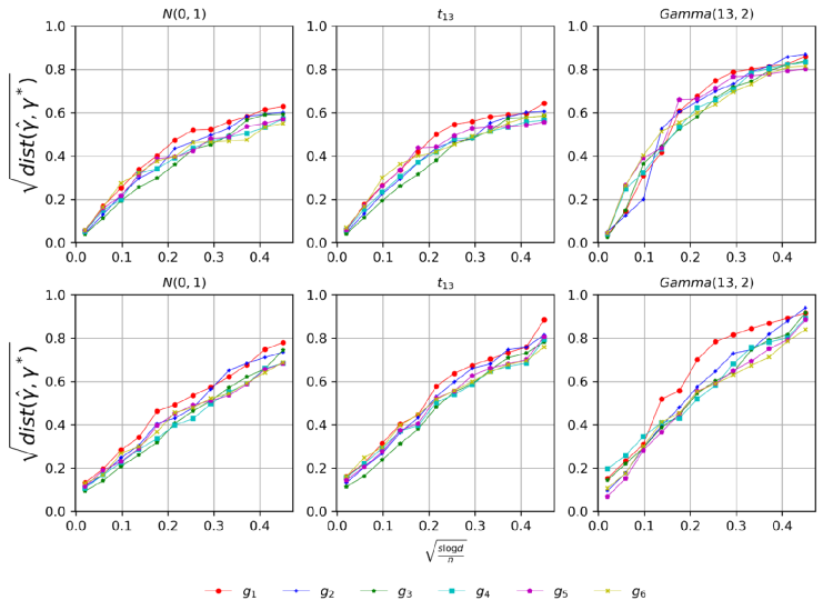
Figure 1: Estimation error for the first-order estimator $\widehat{\bm{\gamma}}_{2}$. The lines indicate different variance functions, while columns indicate different designs on $\mathbf{x}$. The first row corresponds to the setup where score functions are known, while the bottom row to the setup where score functions are estimated by (27).

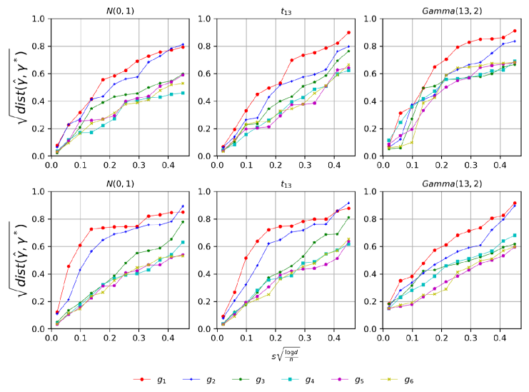
Figure 2: Estimation error for the second-order estimator $\widehat{\bm{\gamma}}_{4}$. Notations are same as Figure 1.

5.2 Multiple index experiment

We consider two estimators of $\bm{G}^{\star}$ here: $\widehat{\bm{G}}_{2}$ and $\widehat{\bm{G}}_{3}$ described in Section 4. We set $d=100$, $s=10$, and $v=3$. We let $\text{supp}(\bm{\gamma}^{\star}_{j})=[(j-1)s,js]$ and each entry in the support is set to $\pm 1/\sqrt{s}$ with equal probability. The variance link function is defined as $g({\bm{G}^{\star}}^{T}\mathbf{x})=\sum_{j=1}^{v}g(\mathbf{x}^{T}\bm{\gamma}^{\star}_{j})$ where $g\in\{g_{i}\}_{i=1}^{6}$ is the variance function used in the single index experiment. In this experiment, we let $\tau=10(n/\log d)^{\frac{1}{6}}$, $\lambda=0.01\sqrt{\log d/n}$. The results are shown in Figures 3 and 4, and again we observe that the error rate is correctly explained by our theory for sufficiently large sample size. In particular, we observe that the error rate is sublinear in term of $s\sqrt{v\log d/n}$ as expected.

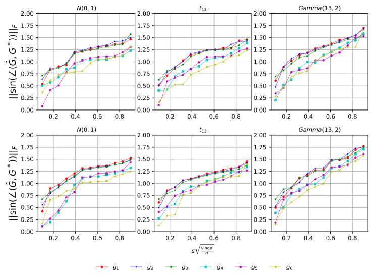
Figure 3: Estimation error for the second-order estimator $\widehat{\bm{G}}_{2}$ (regular case).

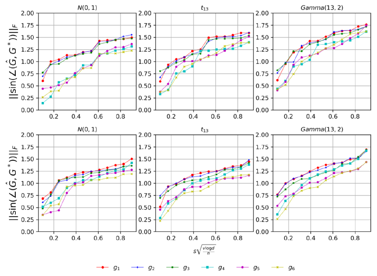
Figure 4: Estimation error for the second-order estimator $\widehat{\bm{G}}_{3}$ (orthogonal case).

6 Discussion

We proposed new estimators for parametric components of index volatility models based on the first- and second-order Stein’s identities. Our approach extracts the direction of variance index by multiplying the score variables with residuals and incorporating weighted mean squared minimization with truncation and regularization to accommodate for estimation in a high-dimensional and heavy-tailed setting. We established statistical rates of convergence of our estimators under both single and multiple index structures, which were then verified in finite samples through numerical experiments. In particular, our results were qualitatively the same under a range of designs, including heavy-tailed ones. The estimation rate is comprised of both nonparametric and parametric rates, though the parametric rate is the dominant term and matches the corresponding rate in the mean estimation. We illustrated that when the mean index is orthogonal to the variance index, which would naturally be the case in many high-dimensional applications, we need not estimate the mean link function and can obtain finite sample results.

Our estimation procedures rely on estimation of the gradient of link function through Stein’s identities, which is aligned with the e.d.r. direction in index volatility models. Using this approach, we were able to naturally extend traditional fixed design setup to randomized design. The drawback of the approach based on Stein’s identity is that the prior knowledge of a distribution of covariates $\mathbf{x}$ is needed. In a low-dimensional setting, Babichev and Bach (2018) proposed an approach for estimating the first-order score function under the assumption that the score function can be represented as a finite linear combination of basis functions in a given dictionary. We implement this approach in our experiments to address practical concerns, however theoretical analysis for extending their approach to a high-dimensional setting seems challenging without strong assumptions on the underlying distribution of $\mathbf{x}$. We leave investigation of possible estimators for future work. Fortunately, in some applications, such as compressed sensing (Ai et al., 2014; Davenport et al., 2014) or phase retrieval (Candès et al., 2015a, b), the distribution of covariates is known.

In this work, we have focused on point estimation of the e.d.r. direction. Establishing tools that would allow for construction of confidence intervals and more generally uncertainty quantification is an important future direction. Another direction is improving the statistical rate obtained by the second-order estimation procedures, which arises from the finite moment condition on $H(\mathbf{x})$ that makes bounding of the restricted operator norm difficult. We note, however, that obtaining the error rate of $\sqrt{s\log d/n}$ under heavy-tailed design for sparse PCA is still an open problem. In addition, developing a robust version of the estimators based on absolute residuals, as used for robust variance estimation (Davidian and Carroll, 1987), would further enlarge potential for diverse applications of our methodology. Finally, it is also of interest to study higher-order methods. Dudeja and Hsu (2018) proposed $l$-th order estimator based on Hermite polynomials, and proved that the rate of convergence is $\sqrt{d(\log d)^{l}/n}$. This is useful especially when $\mu_{1}=\mu_{2}=0$. Analogously and to deal with non-Gaussian design, one can recursively define higher-order score variable $S_{l}(\mathbf{x})=-S_{l-1}(\mathbf{x})\otimes\nabla\log p(\mathbf{x})+\nabla S_{l-1}(\mathbf{x})$ and use higher-order Stein’s identity, $\mathbb{E}[f(\mathbf{x}^{T}\bm{\beta}^{\star})S_{l}(\mathbf{x})]=f^{(l)}(\mathbf{x}^{T}\bm{\beta}^{\star})\cdot(\bm{\beta}^{\star})^{\otimes l}$, to estimate the index. However, this may require tensor decomposition and is less efficient than the nonconvex method in Dudeja and Hsu (2018). How to bridge this computational gap and have an efficient higher-order estimator with optimal convergence rate is an attractive topic for future work.

Supplemental Materials:
High-dimensional Index Volatility Models via Stein’s Identity

Appendix A Estimation of Index Mean Function

In this section, we present results on the mean estimation for the model (1). In particular, we develop an explicit formula for $\bar{e}_{f}(\widehat{\bm{\beta}}^{T}\mathbf{x},n,1)$ in (9), and further derive a bound on its first moment, $\widehat{e}_{f}(\widehat{\bm{\beta}},n,1)$, and error rate $\widetilde{e}_{f,\delta}(n,1)$. By Corollary 2.7 we finally verify the argument in (11). Our estimation procedure is based on two steps. First, we use the approach in Yang et al. (2017a) to estimate the mean index $\bm{\beta}^{\star}$. Next, a local linear regression is applied on the pair $(y,\widehat{\bm{\beta}}^{T}\mathbf{x})$ to obtain the mean link function estimator $\widehat{f}$. Finally, we use $\widehat{f}(\langle\widehat{\bm{\beta}},\mathbf{x}\rangle)$ as an estimation of $f(\langle\bm{\beta}^{\star},\mathbf{x}\rangle)$. To simplify the analysis, we assume that two steps are conducted on independent samples of size $n$ for each, which is obtained, for example, by sample splitting in practice. This simplifies the analysis while keeping the statistical rate unchanged. We note that the local linear regression is just one way to estimate the nonparametric component in index models. See Liu et al. (2013) for a robust estimator as an alternative.

To unify the presentation, we consider a more general heteroscedastic index model:

$$y\mid\mathbf{x}=f(\langle\bm{\beta}^{\star},\mathbf{x}\rangle)+\widetilde{g}(\mathbf{x})\epsilon,$$ (A.1)

where $\mathbb{E}[\epsilon|\mathbf{x}]=0$, $\mathbb{E}[\epsilon^{2}|\mathbf{x}]=1$. By setting $\widetilde{g}(\mathbf{x})=g(\langle\bm{\gamma}^{\star},\mathbf{x}\rangle)$ we obtain the single index volatility model and $\widetilde{g}(\mathbf{x})=g({\bm{G}^{\star}}^{T}\mathbf{x})$ would lead to multiple index volatility model. The estimator $\widehat{\bm{\beta}}$ in Yang et al. (2017a) is defined as

$$\widehat{\bm{\beta}}=\phi_{\lambda}\bigg{(}\frac{1}{n}\sum_{i=1}^{n}\Psi_{\tau}(y_{i})\Psi_{\tau}(S(\mathbf{x}_{i}))\bigg{)},$$ (A.2)

where $\lambda$ and $\tau$ are tuning parameters. This Lasso-type estimator comes from the first-order Stein’s identity applied on the response $y$. Here $\tau$ is the truncation threshold and $\lambda$ controls the sparsity of $\widehat{\bm{\beta}}$. Note that $\widehat{\bm{\beta}}$ can be computed without the knowledge of $f$. Its convergence rate is presented in the following theorem.

Theorem A.1 ($\bm{\beta}^{\star}$ estimation).

Suppose the function $f(\langle\bm{\beta}^{\star},\mathbf{x}\rangle)$ together with $\mathbf{x}$ satisfies the first-order regularity condition. Furthermore, suppose Assumption 2.5 holds with $p\geq 4$ and $\|\bm{\beta}^{\star}\|_{0}\leq s$. Then, for any $0<\delta<1$, the estimator $\widehat{\bm{\beta}}$ defined in (A.2) for $\bm{\beta}^{\star}$ in model (A.1), with $\lambda\asymp\sqrt{\log(d/\delta)/n}$ and $\tau\asymp(n/\log(d/\delta))^{1/4}$, satisfies

$$\|\widehat{\bm{\beta}}-\bm{\beta}^{\star}\|_{2}\lesssim\sqrt{\frac{s\log(d/\delta)}{n}},\quad\|\widehat{\bm{\beta}}-\bm{\beta}^{\star}\|_{1}\lesssim s\sqrt{\frac{\log(d/\delta)}{n}},\quad\|\widehat{\bm{\beta}}-\bm{\beta}^{\star}\|_{\infty}\lesssim\sqrt{\frac{\log(d/\delta)}{n}},$$

with probability at least $1-\delta$.

Theorem 4.2 in Yang et al. (2017a) proves the above result for a high-dimensional homoscedastic single index model. Theorem A.1 states a more general result that is valid for a heteroscedastic single index model. The proof is omitted as the proof strategy of Yang et al. (2017a) is directly applicable, since

$$\mathbb{E}[yS(\mathbf{x})]=\mathbb{E}[f(\langle\bm{\beta}^{\star},\mathbf{x}\rangle)S(\mathbf{x})]+\mathbb{E}[\epsilon\widetilde{g}(\mathbf{x})S(\mathbf{x})]=\mathbb{E}[f(\langle\bm{\beta}^{\star},\mathbf{x}\rangle)S(\mathbf{x})]=c\bm{\beta}^{\star}.$$

With $\widehat{\bm{\beta}}$ defined above, we use a local linear regression estimator to estimate $f(\cdot)$. The results borrows from Fan (1993) and requires the following assumption (see Condition 1 in Fan (1993) for comparison). The assumption is specifically required for estimation using local linear regression and would need to be adjusted if other estimators are used.

Assumption A.2.

For any fixed estimator $\widehat{\bm{\beta}}$ with the rate of convergence as in Theorem A.1, we assume

1. (smoothness) $f\in C^{2}(\mathbb{R})$ with $|f^{\prime}(x)|\vee|f^{\prime\prime}(x)|\leq L_{1}$, $\forall x\in\mathbb{R}$.

2. ($4$th moment function) $r_{\widehat{\bm{\beta}}}(x)=\mathbb{E}[\widetilde{g}^{4}(\mathbf{x})\mid\widehat{\bm{\beta}}^{T}\mathbf{x}=x]$ is continuous and bounded.

3. (density) $\widehat{\bm{\beta}}^{T}\mathbf{x}$ has bounded positive density $q_{\widehat{\bm{\beta}}}$ with $|q_{\widehat{\bm{\beta}}}(x)-q_{\widehat{\bm{\beta}}}(y)|\leq L_{2}|x-y|^{\alpha}$ for $\alpha\in(0,1)$.

4. (tail) there exists a constant $L_{3}>0$ such that $|f(x)|^{4}/q_{\widehat{\bm{\beta}}}^{8}(x)$, $r_{\widehat{\bm{\beta}}}(x)/q_{\widehat{\bm{\beta}}}(x)$, and $|f^{\prime}(x)|^{4}/q_{\widehat{\bm{\beta}}}(x)$ are integrable on $(-\infty,-L_{3})\cup(L_{3},\infty)$.

With these assumptions, we define the local linear estimator as

$$\widehat{f}(t)=\frac{\sum_{i=1}^{n}w_{i}y_{i}}{\sum_{i=1}^{n}w_{i}+(nh)^{-2}},$$ (A.3)

where $w_{i}=K_{h}(\mathbf{x}_{i}^{T}\widehat{\bm{\beta}}-t)\big{(}s_{n2}-(\mathbf{x}_{i}^{T}\widehat{\bm{\beta}}-t)\cdot s_{n1}\big{)}$ with $s_{nl}=\sum_{i=1}^{n}K_{h}(\mathbf{x}_{i}^{T}\widehat{\bm{\beta}}-t)(\mathbf{x}_{i}^{T}\widehat{\bm{\beta}}-t)^{l}$ for $l=1,2$, $h$ is the bandwidth, and $K_{h}(\cdot)=K(\cdot/h)/h$ for a kernel function $K(\cdot)$. With a Gaussian kernel, we have the following rate of convergence for the mean estimator.

Theorem A.3 (Mean estimation).

Suppose $\widehat{\bm{\beta}}$ is estimated using samples $\mathcal{D}_{1}$ and satisfies the rate in Theorem A.1. Given $\widehat{\bm{\beta}}$, let $\widehat{f}$, defined in (A.3), be a local linear estimator of the link function $f$ using samples $\mathcal{D}_{2}=\{y_{i},\widehat{\bm{\beta}}^{T}\mathbf{x}_{i}\}_{i\in[n]}$ that are independent from $\mathcal{D}_{1}$. Suppose Assumption 2.5 with $p\geq 4$ and Assumption A.2 (a-c) hold and the bandwidth $h$ satisfies $h\rightarrow 0$ and $nh\rightarrow\infty$. Then there exist $N$ and $\Upsilon_{1}$ such that $\forall n\geq N$,

$$\mathbb{E}[|\widehat{f}(\mathbf{x}^{T}\widehat{\bm{\beta}})-f(\mathbf{x}^{T}\bm{\beta}^{\star})|^{4}\mid\mathbf{x},\mathcal{D}_{1}]\leq\Upsilon_{1}\bigg{(}h^{8}+ \frac{r_{\widehat{\bm{\beta}}}(\mathbf{x}^{T}\widehat{\bm{\beta}})}{n^{2}h^{2}q_{\widehat{\bm{\beta}}}^{2}(\mathbf{x}^{T}\widehat{\bm{\beta}})}+\frac{\|\widehat{\bm{\beta}}-\bm{\beta}^{\star}\|_{2}^{4}\cdot|f^{\prime}(\mathbf{x}^{T}\widehat{\bm{\beta}})|^{4}}{h^{2}q_{\widehat{\bm{\beta}}}^{2}(\mathbf{x}^{T}\widehat{\bm{\beta}})}$$

$$+ |\mathbf{x}^{T}\bm{\beta}^{\star}-\mathbf{x}^{T}\widehat{\bm{\beta}}|^{4}+\frac{|f(\mathbf{x}^{T}\widehat{\bm{\beta}})|^{4}}{n^{16}h^{16}q_{\widehat{\bm{\beta}}}^{8}(\mathbf{x}^{T}\widehat{\bm{\beta}})}\bigg{)}.$$ (A.4)

Furthermore, suppose Assumption A.2 (d) holds as well and $h\asymp n^{-1/5}$, then there exists a constant $\Upsilon_{2}$ such that

$$P\bigg{(}\biggl{\|}\mathbb{E}\big{[}|\widehat{f}(\mathbf{x}^{T}\widehat{\bm{\beta}})-f(\mathbf{x}^{T}\bm{\beta}^{\star})|^{2}\cdot W(\mathbf{x})\mid\mathcal{D}_{1},\mathcal{D}_{2}\big{]}\biggr{\|}_{\infty}\geq\frac{\sqrt{M_{2}}}{\delta}\underbrace{\Upsilon_{2}n^{-4/5}}_{\widetilde{e}_{f,\delta}(n,1)}\bigg{)}\leq 2\delta,$$ (A.5)

where $W(\mathbf{x})$ is either the first-order score variable $S(\mathbf{x})$ or the second-order score variable $H(\mathbf{x})$.

We see equation (A.3) provides an explicit form of $\bar{e}_{f}(\widehat{\bm{\beta}}^{T}\mathbf{x},n,1)$ in (9). We explicitly write out higher-order terms in (A.3) to clarify the difference between a high-dimensional single index model and a nonparametric model. In a low-dimensional setting with $\mathbf{x}$ being in a compact set and $q_{\widehat{\bm{\beta}}}$ lower bounded away from zero (Zhu and Xue, 2006; Van Keilegom and Wang, 2010; Wang et al., 2010; Lian et al., 2015), the last two terms can be ignored.

As discussed in Section 2, estimation of $\bm{G}^{\star}$ is possible under a heavy-tailed design if condition (10) holds. Assumption A.2 (d) implies that expectation of the right hand side of (A.3), conditional on $\widehat{\bm{\beta}}$, is bounded on the tails; while within the interval $[-L_{3},L_{3}]$, we can make use of continuity so that the integral is bounded naturally. In particular, the assumption imposes conditions on the decay rate of $|f(x)|$, $|f^{\prime}(x)|$, and $r_{\widehat{\bm{\beta}}}(x)$, and holds for any random variables that have compact support. Taking conditional expectation for $\bar{e}_{f}(\widehat{\bm{\beta}}^{T}\mathbf{x},n,1)$ and ignoring all smaller order terms, we have

$$\widehat{e}_{f}(\widehat{\bm{\beta}},n,1)\lesssim h^{8}+\frac{1}{n^{2}h^{2}}+\frac{\|\widehat{\bm{\beta}}-\bm{\beta}^{\star}\|_{2}^{4}}{h^{2}}.$$

Moreover, using the fact that $\|\widehat{\bm{\beta}}-\bm{\beta}^{\star}\|_{2}\lesssim 1/\sqrt{n}$, we can set the bandwidth $h\asymp n^{-1/5}$ to obtain $\widetilde{e}_{f,\delta}(n,1)\lesssim n^{-4/5}$.

We also point out that $L_{2}$ and $L_{3}$ in Assumption A.2 (c-d) do not depend on $\widehat{\bm{\beta}}$ as long as it is close to $\bm{\beta}^{\star}$, which is assumed similarly in Zhang (2018). An equivalent statement would be to assume $q_{\bm{\beta}^{\star}},r_{\bm{\beta}^{\star}}$ satisfy conditions (c-d) and further add some continuity conditions on $q_{\bm{\beta}^{\star}},r_{\bm{\beta}^{\star}}$ with respect to $\bm{\beta}$, such that $|q_{\widehat{\bm{\beta}}}-q_{\bm{\beta}^{\star}}|$ and $|r_{\widehat{\bm{\beta}}}-r_{\bm{\beta}^{\star}}|$ are small enough. For example, suppose $|q_{\widehat{\bm{\beta}}}(x)-q_{\widehat{\bm{\beta}}}(x)|\leq L_{x}\|\widehat{\bm{\beta}}-\bm{\beta}^{\star}\|_{2}$ and $\sup_{x}L_{x}<\infty$, then by triangle inequality we have $\forall x,y$

$$|q_{\widehat{\bm{\beta}}}(x)-q_{\widehat{\bm{\beta}}}(y)|\leq |q_{\widehat{\bm{\beta}}}(x)-q_{\bm{\beta}^{\star}}(x)|+|q_{\bm{\beta}^{\star}}(x)+q_{\bm{\beta}^{\star}}(y)|+|q_{\widehat{\bm{\beta}}}(y)-q_{\bm{\beta}^{\star}}(y)|$$

$$\leq \underbrace{2\sup_{x}L_{x}\|\widehat{\bm{\beta}}-\bm{\beta}^{\star}\|_{2}}_{\text{ignorable}}+L_{3}|x-y|^{\alpha}\lesssim L_{3}^{\prime}|x-y|^{\alpha}.$$

Appendix B Proofs of Main Theorems and Lemmas

Throughout this section, we write $M$, omitting the subscript of $M_{p}$, since the moment degree $p$ is clear from the statement of theorem. For simplicity, we replace the truncation function $\Psi_{\tau}$ by notation $\widecheck{(\cdot)}$ where the truncation threshold $\tau$ is contained implicitly. In particular, we have $\Psi_{\tau}(\bm{v})=\widecheck{\bm{v}}$. We use $\Upsilon>0$ to denote a generic constant, which may take different values for each appearance. For Theorem 3.2, 3.3, 3.4, 3.6, 4.1, 4.2, we only prove the first part of statement since the second part is trivial to obtain by plugging in $\widetilde{e}_{f,\delta}(n,1)\asymp n^{-4/5}$.

B.1 Proof of Theorem 2.6

We prove the result for $W(\mathbf{x})=S(\mathbf{x})$ as the other case is shown analogously. For any $j\in[d]$,

$$\mathbb{E}_{\widehat{f}}\big{[}|\widehat{f}(\mathbf{x})-f(\mathbf{x})|^{2}\cdot|S(\mathbf{x})_{j}|\big{]}\leq \sqrt{\mathbb{E}_{\widehat{f}}\big{[}|\widehat{f}(\mathbf{x})-f(\mathbf{x})|^{4}\big{]}}\sqrt{\mathbb{E}[|S(\mathbf{x})_{j}|^{2}]}$$

$$\leq \sqrt{M}\sqrt{\mathbb{E}_{\widehat{f}}\big{[}|\widehat{f}(\mathbf{x})-f(\mathbf{x})|^{4}\big{]}}.$$

Therefore, we have

$$\big{\|}\mathbb{E}_{\widehat{f}}\big{[}|\widehat{f}(\mathbf{x})-f(\mathbf{x})|^{2}\cdot S(\mathbf{x})\big{]}\big{\|}_{\infty}\leq\sqrt{M}\sqrt{\mathbb{E}_{\widehat{f}}\big{[}|\widehat{f}(\mathbf{x})-f(\mathbf{x})|^{4}\big{]}}.$$

By Markov’s inequality, for any $0<\delta<1$, with probability $1-\delta$, we have

$$\sqrt{\mathbb{E}_{\widehat{f}}\big{[}|\widehat{f}(\mathbf{x})-f(\mathbf{x})|^{4}\big{]}}\leq\sqrt{\frac{\mathbb{E}[|\widehat{f}(\mathbf{x})-f(\mathbf{x})|^{4}]}{\delta}}\stackrel{{\scriptstyle(\ref{cond:3})}}{{\leq}}\frac{\widetilde{e}_{f}(n,d)}{\delta}.$$

Combining the above two inequalities completes the proof.

B.2 Proof of Corollary 2.7

Similar to the proof of Theorem 2.6, we have for any $j\in[d]$,

$$\mathbb{E}_{\widehat{\bm{\beta}},\widehat{f}}\big{[}|\widehat{f}(\mathbf{x}^{T}\widehat{\bm{\beta}})-f(\mathbf{x}^{T}\bm{\beta}^{\star})|^{2}\cdot|S(\mathbf{x})_{j}|\big{]}\leq \sqrt{\mathbb{E}_{\widehat{\bm{\beta}},\widehat{f}}\big{[}|\widehat{f}(\mathbf{x}^{T}\widehat{\bm{\beta}})-f(\mathbf{x}^{T}\bm{\beta}^{\star})|^{4}\big{]}}\sqrt{\mathbb{E}[|S(\mathbf{x})_{j}|^{2}]}$$

$$\leq \sqrt{M}\sqrt{\mathbb{E}_{\widehat{\bm{\beta}},\widehat{f}}\big{[}|\widehat{f}(\mathbf{x}^{T}\widehat{\bm{\beta}})-f(\mathbf{x}^{T}\bm{\beta}^{\star})|^{4}\big{]}}$$

and

$$\big{\|}\mathbb{E}_{\widehat{\bm{\beta}},\widehat{f}}\big{[}|\widehat{f}(\mathbf{x}^{T}\widehat{\bm{\beta}})-f(\mathbf{x}^{T}\bm{\beta}^{\star})|^{2}\cdot|S(\mathbf{x})_{j}|\big{]}\big{\|}_{\infty}\leq\sqrt{M}\sqrt{\mathbb{E}_{\widehat{\bm{\beta}},\widehat{f}}\big{[}|\widehat{f}(\mathbf{x}^{T}\widehat{\bm{\beta}})-f(\mathbf{x}^{T}\bm{\beta}^{\star})|^{4}\big{]}}.$$

By Markov’s inequality, for any $0<\delta<1$ and any sample set $\mathcal{D}_{1}$,

$$P\bigg{(}\mathbb{E}_{\widehat{\bm{\beta}},\widehat{f}}\big{[}|\widehat{f}(\mathbf{x}^{T}\widehat{\bm{\beta}})-f(\mathbf{x}^{T}\bm{\beta}^{\star})|^{4}\big{]}\leq\frac{\mathbb{E}_{\widehat{\bm{\beta}}}\big{[}|\widehat{f}(\mathbf{x}^{T}\widehat{\bm{\beta}})-f(\mathbf{x}^{T}\bm{\beta}^{\star})|^{4}\big{]}}{\delta}\mathrel{\bigg{|}}\mathcal{D}_{1}\bigg{)}\geq 1-\delta,$$ (B.1)

where the probability is taken over randomness in $\mathcal{D}_{2}$. By the definition in (9), we have

$$P\bigg{(}\sqrt{\mathbb{E}_{\widehat{\bm{\beta}},\widehat{f}}\big{[}|\widehat{f}(\mathbf{x}^{T}\widehat{\bm{\beta}})-f(\mathbf{x}^{T}\bm{\beta}^{\star})|^{4}\big{]}}\leq\sqrt{\widehat{e}_{f}(\widehat{\bm{\beta}},n,1)}/\delta\mathrel{\bigg{|}}\mathcal{D}_{1}\bigg{)}\geq 1-\delta.$$

Under the condition (10), we have

$$P\bigg{(}\bigg{\|} \mathbb{E}_{\widehat{\bm{\beta}},\widehat{f}}\big{[}|\widehat{f}(\mathbf{x}^{T}\widehat{\bm{\beta}})-f(\mathbf{x}^{T}\bm{\beta}^{\star})|^{2}\cdot|S(\mathbf{x})_{j}|\big{]}\bigg{\|}_{\infty}\geq\frac{\sqrt{M}\cdot\widetilde{e}_{f,\delta}(n,1)}{\delta}\bigg{)}$$

$$\leq P\bigg{(}\sqrt{\mathbb{E}_{\widehat{\bm{\beta}},\widehat{f}}\big{[}|\widehat{f}(\mathbf{x}^{T}\widehat{\bm{\beta}})-f(\mathbf{x}^{T}\bm{\beta}^{\star})|^{4}\big{]}}\geq\widetilde{e}_{f,\delta}(n,1)/\delta\bigg{)}$$

$$\leq P\bigg{(}\sqrt{\mathbb{E}_{\widehat{\bm{\beta}},\widehat{f}}\big{[}|\widehat{f}(\mathbf{x}^{T}\widehat{\bm{\beta}})-f(\mathbf{x}^{T}\bm{\beta}^{\star})|^{4}\big{]}}\geq\sqrt{\widehat{e}_{f}(\widehat{\bm{\beta}},n,1)}/\delta\text{\ or\ }\sqrt{\widehat{e}_{f}(\widehat{\bm{\beta}},n,1)}\geq\widetilde{e}_{f,\delta}(n,1)\bigg{)}$$

$$\leq P\bigg{(}\sqrt{\mathbb{E}_{\widehat{\bm{\beta}},\widehat{f}}\big{[}|\widehat{f}(\mathbf{x}^{T}\widehat{\bm{\beta}})-f(\mathbf{x}^{T}\bm{\beta}^{\star})|^{4}\big{]}}\geq\sqrt{\widehat{e}_{f}(\widehat{\bm{\beta}},n,1)}/\delta\bigg{)}+P\bigg{(}\sqrt{\widehat{e}_{f}(\widehat{\bm{\beta}},n,1)}\geq\widetilde{e}_{f,\delta}(n,1)\bigg{)}$$

$$\stackrel{{\scriptstyle\eqref{cond:6}}}{{\leq}} \delta+\int P\bigg{(}\sqrt{\mathbb{E}_{\widehat{\bm{\beta}},\widehat{f}}\big{[}|\widehat{f}(\mathbf{x}^{T}\widehat{\bm{\beta}})-f(\mathbf{x}^{T}\bm{\beta}^{\star})|^{4}\big{]}}\geq\sqrt{\widehat{e}_{f}(\widehat{\bm{\beta}},n,1)}/\delta\mathrel{\bigg{|}}\mathcal{D}_{1}\bigg{)}\underbrace{dP(\mathcal{D}_{1})}_{\begin{subarray}{c}\text{take integral over}\\ \\ \text{randomness in }\mathcal{D}_{1}\end{subarray}}$$

$$\leq 2\delta.$$

Here the last inequality is due to the fact that $\mathcal{D}_{1}$ and $\mathcal{D}_{2}$ are independent, so (B.1) holds uniformly for any $\mathcal{D}_{1}$.

B.3 Proof of Theorem 3.2

Since the samples used for estimating $\widetilde{\bm{\gamma}}$ are independent from $\widehat{f}$, $\widehat{\bm{\beta}}$,

$$\mathbb{E}_{\widehat{\bm{\beta}},\widehat{f}}[(y-\widehat{f}(\mathbf{x}^{T}\widehat{\bm{\beta}}))^{2}\cdot S(\mathbf{x})] =\mathbb{E}_{\widehat{\bm{\beta}},\widehat{f}}[(y-f(\mathbf{x}^{T}\bm{\beta}^{\star})+f(\mathbf{x}^{T}\bm{\beta}^{\star})-\widehat{f}(\mathbf{x}^{T}\widehat{\bm{\beta}}))^{2}\cdot S(\mathbf{x})]$$

$$=\mathbb{E}[g^{2}(\mathbf{x}^{T}\bm{\gamma}^{\star})S(\mathbf{x})]+\mathbb{E}_{\widehat{\bm{\beta}},\widehat{f}}[(f(\mathbf{x}^{T}\bm{\beta}^{\star})-\widehat{f}(\mathbf{x}^{T}\widehat{\bm{\beta}}))^{2}\cdot S(\mathbf{x})]$$

$$\stackrel{{\scriptstyle\eqref{equ:1}}}{{=}}\widetilde{\bm{\gamma}}+\mathbb{E}_{\widehat{\bm{\beta}},\widehat{f}}[(f(\mathbf{x}^{T}\bm{\beta}^{\star})-\widehat{f}(\mathbf{x}^{T}\widehat{\bm{\beta}}))^{2}\cdot S(\mathbf{x})].$$ (B.2)

For the second term, according to (11), for any $\delta>0$

$$P\bigg{(}\biggl{\|}\mathbb{E}_{\widehat{\bm{\beta}},\widehat{f}}\big{[}|\widehat{f}(\langle\widehat{\bm{\beta}},\mathbf{x}\rangle)-f(\langle\bm{\beta}^{\star},\mathbf{x}\rangle)|^{2}\cdot S(\mathbf{x})\big{]}\biggr{\|}_{\infty}\geq\frac{\sqrt{M}\cdot\widetilde{e}_{f,\delta}(n,1)}{\delta}\bigg{)}\leq 2\delta.$$ (B.3)

(Here $M$ refers to $M_{6}$ since $\sqrt{M_{2}}\leq\sqrt{M_{6}}$.) Next, we bound the error that occurs when using $\widehat{\bm{\gamma}}_{1}$ to approximate the left hand side term in (B.3). We apply Lemma C.2. Based on Assumption 2.5 ($p\geq 6$) we know that for some constant $\Upsilon_{1}$

$$\mathbb{E}[|y|^{6}]\vee\mathbb{E}[|S(\mathbf{x})_{j}|^{6}]\vee\mathbb{E}[|f({\bm{\beta}^{\star}}^{T}\mathbf{x})|^{6}]\leq\Upsilon_{1}M,\text{\ \ }\forall j\in[d].$$

Furthermore, by Markov’s inequality, for any $\delta>0$, we have

$$\mathbb{E}_{\widehat{\bm{\beta}},\widehat{f}}[|\widehat{f}(\mathbf{x}^{T}\widehat{\bm{\beta}})|^{6}]\leq \frac{32}{\delta}\mathbb{E}[|\widehat{f}(\mathbf{x}^{T}\widehat{\bm{\beta}})-f(\mathbf{x}^{T}\widehat{\bm{\beta}})|^{6}]+32\mathbb{E}_{\widehat{\bm{\beta}}}[|f(\mathbf{x}^{T}\widehat{\bm{\beta}})|^{6}]$$

with probability $1-\delta$. The first term goes to zero as $n\rightarrow\infty$ and it only attributes to higher order errors. Thus, there exists $N_{\delta}$ such that $\forall n\geq N_{\delta}$

$$\frac{32\mathbb{E}[|\widehat{f}(\mathbf{x}^{T}\widehat{\bm{\beta}})-f(\mathbf{x}^{T}\widehat{\bm{\beta}})|^{6}]}{\delta}\leq\frac{\Upsilon_{1}M}{2}.$$

Roughly, by nonparametric rate, we only require $\frac{1}{\delta n^{p}}\leq M$, which implies $n\geq(\frac{1}{\delta M})^{\frac{1}{p}}\eqqcolon N_{\delta}$ for some $p>1$. From Lemma C.1, we also have $\mathbb{E}_{\widehat{\bm{\beta}}}[|f(\mathbf{x}^{T}\widehat{\bm{\beta}})|^{6}]\leq\frac{\Upsilon_{1}M}{64}$ for a sufficiently large $N$ (not depending on $\delta$) and $\Upsilon_{1}$. Combining them together, we have $\mathbb{E}_{\widehat{\bm{\beta}},\widehat{f}}[|\widehat{f}(\mathbf{x}^{T}\widehat{\bm{\beta}})|^{6}]\leq\Upsilon_{1}M$ with probability $1-\delta$. Based on the definition of $\widehat{\bm{\gamma}}_{1}$ in (15),

$$\|\widehat{\bm{\gamma}}_{1}- \mathbb{E}_{\widehat{\bm{\beta}},\widehat{f}}[(y-\widehat{f}(\mathbf{x}^{T}\widehat{\bm{\beta}}))^{2}\cdot S(\mathbf{x})]\|_{\infty}$$

$$\leq \biggl{\|}\frac{1}{n}\sum_{i=1}^{n}\widecheck{y_{i}}^{2}\widecheck{S(\mathbf{x}_{i})}-\mathbb{E}_{\widehat{\bm{\beta}},\widehat{f}}[y^{2}S(\mathbf{x})]\biggr{\|}_{\infty}+2\biggl{\|}\frac{1}{n}\sum_{i=1}^{n}\widecheck{y_{i}}\widecheck{\widehat{f}(\mathbf{x}_{i}^{T}\widehat{\bm{\beta}})}\widecheck{S(\mathbf{x}_{i})}-\mathbb{E}_{\widehat{\bm{\beta}},\widehat{f}}[y\widehat{f}(\mathbf{x}^{T}\widehat{\bm{\beta}})S(\mathbf{x})]\biggr{\|}_{\infty}$$

$$+\biggl{\|}\frac{1}{n}\sum_{i=1}^{n}\widecheck{\widehat{f}(\mathbf{x}_{i}^{T}\widehat{\bm{\beta}})}^{2}\widecheck{S(\mathbf{x}_{i})}-\mathbb{E}_{\widehat{\bm{\beta}},\widehat{f}}[\widehat{f}(\mathbf{x}^{T}\widehat{\bm{\beta}})S(\mathbf{x})]\biggr{\|}_{\infty}.$$

For the above each term, applying Lemma C.2, setting $\tau=(\frac{n\Upsilon_{1}M}{\log(2d/\delta)})^{\frac{1}{6}}$ and taking union bound over all $d$ indices, we obtain

$$P\bigg{(}\biggr{\|}\widehat{\bm{\gamma}}_{1}-\mathbb{E}_{\widehat{\bm{\beta}},\widehat{f}}[(y-\widehat{f}(\mathbf{x}^{T}\widehat{\bm{\beta}}))^{2}S(\mathbf{x})]\biggl{\|}_{\infty}\leq 28\sqrt{\frac{\Upsilon_{1}M\log(2d/\delta)}{n}}\bigg{)}\geq 1-4\delta.$$ (B.4)

Combining (B.3), (B.3) and (B.4) together and adjusting $\delta$ properly, we know there exists constant $\Upsilon$ large enough such that, by setting $\tau=\Upsilon(\frac{nM}{\log(d/\delta)})^{\frac{1}{6}}$,

$$\|\widehat{\bm{\gamma}}_{1}-\widetilde{\bm{\gamma}}\|_{\infty}\leq \|\widehat{\bm{\gamma}}_{1}-\mathbb{E}_{\widehat{\bm{\beta}},\widehat{f}}[(y-\widehat{f}(\mathbf{x}^{T}\widehat{\bm{\beta}}))^{2}S(\mathbf{x})]\|_{\infty}+\|\mathbb{E}_{\widehat{\bm{\beta}},\widehat{f}}[(f(\mathbf{x}^{T}\bm{\beta}^{\star})-\widehat{f}(\mathbf{x}^{T}\widehat{\bm{\beta}}))^{2}S(\mathbf{x})]\|_{\infty}$$

$$\leq \Upsilon\bigg{(}\sqrt{\frac{M\log(d/\delta)}{n}}+\frac{\sqrt{M}\cdot\widetilde{e}_{f,\delta}(n,1)}{\delta}\bigg{)}$$ (B.5)

with probability at least $1-\delta$. This completes the first part of the proof.

Moreover, since $\|\widehat{\bm{\gamma}}_{1}-\widetilde{\bm{\gamma}}\|_{2}\leq\sqrt{d}\|\widehat{\bm{\gamma}}_{1}-\widetilde{\bm{\gamma}}\|_{\infty}$, we know that

$$P\bigg{(}\|\widehat{\bm{\gamma}}_{1}-\widetilde{\bm{\gamma}}\|_{2}\leq\Upsilon\big{(}\sqrt{\frac{Md\log(12d/\delta)}{n}}+\frac{\sqrt{Md}\cdot\widetilde{e}_{f,\delta}(n,1)}{\delta}\big{)}\bigg{)}\geq 1-\delta.$$ (B.6)

Plugging in $\widetilde{e}_{f,\delta}(n,1)\asymp n^{-4/5}$, we see that the latter rate is negligible. Thus, it suffices to show $\text{dist}(\widehat{\bm{\gamma}}_{1},\bm{\gamma}^{\star})\lesssim\frac{1}{\mu_{1}^{2}}\|\widehat{\bm{\gamma}}_{1}-\widetilde{\bm{\gamma}}\|_{2}^{2}$. In fact, because $\|\bm{\gamma}^{\star}\|_{2}=1$,

$$\text{dist}(\widehat{\bm{\gamma}}_{1},\bm{\gamma}^{\star})= 1-\frac{|\widehat{\bm{\gamma}}_{1}^{T}\bm{\gamma}^{\star}|}{\|\widehat{\bm{\gamma}}_{1}\|_{2}}=1-\frac{1}{2|\mu_{1}|\|\widehat{\bm{\gamma}}_{1}\|_{2}}\big{|}\|\widetilde{\bm{\gamma}}\|_{2}^{2}+\|\widehat{\bm{\gamma}}_{1}\|_{2}^{2}-\|\widehat{\bm{\gamma}}_{1}-\widetilde{\bm{\gamma}}\|_{2}^{2}\big{|}$$

$$\leq \bigg{(}1-\frac{|\mu_{1}|}{2\|\widehat{\bm{\gamma}}_{1}\|_{2}}-\frac{\|\widehat{\bm{\gamma}}_{1}\|_{2}}{2|\mu_{1}|}\bigg{)}+\frac{1}{2|\mu_{1}|\|\widehat{\bm{\gamma}}_{1}\|_{2}}\cdot\|\widehat{\bm{\gamma}}_{1}-\widetilde{\bm{\gamma}}\|_{2}^{2}$$

$$\leq \frac{1}{2|\mu_{1}|^{2}}\cdot\|\widehat{\bm{\gamma}}_{1}-\widetilde{\bm{\gamma}}\|_{2}^{2}\cdot\frac{|\mu_{1}|}{\|\widehat{\bm{\gamma}}_{1}\|_{2}}.$$ (B.7)

Note that

$$|\mu_{1}|-\|\widehat{\bm{\gamma}}_{1}-\widetilde{\bm{\gamma}}\|_{2}\leq\|\widehat{\bm{\gamma}}_{1}\|_{2}\leq|\mu_{1}|+\|\widehat{\bm{\gamma}}_{1}-\widetilde{\bm{\gamma}}\|_{2},$$

hence we have ($\|\widehat{\bm{\gamma}}_{1}-\widetilde{\bm{\gamma}}\|_{2}/|\mu_{1}|\leq 1/2$)

$$1-\frac{\|\widehat{\bm{\gamma}}_{1}-\widetilde{\bm{\gamma}}\|_{2}}{|\mu_{1}|}\leq \frac{|\mu_{1}|}{\|\widehat{\bm{\gamma}}_{1}\|}\leq 1+\frac{2\|\widehat{\bm{\gamma}}_{1}-\widetilde{\bm{\gamma}}\|_{2}}{|\mu_{1}|}.$$

Plugging back into (B.3) concludes the proof.

B.4 Proof of Theorem 3.3

We start from the definition of $\widehat{\bm{\gamma}}_{2}$ in (16). From the basic inequality, we know

$$\frac{1}{2}\|\widehat{\bm{\gamma}}_{2}\|^{2}-\langle\widehat{\bm{\gamma}}_{2},\widehat{\bm{\gamma}}_{1}\rangle+\lambda\|\widehat{\bm{\gamma}}_{2}\|_{1}\leq\frac{1}{2}\|\widetilde{\bm{\gamma}}\|^{2}-\langle\widetilde{\bm{\gamma}},\widehat{\bm{\gamma}}_{1}\rangle+\lambda\|\widetilde{\bm{\gamma}}\|_{1}.$$

Define $\bm{\Delta}=\widehat{\bm{\gamma}}_{2}-\widetilde{\bm{\gamma}}$ and $\omega=\text{supp}(\widetilde{\bm{\gamma}})=\text{supp}(\bm{\gamma}^{\star})$, then

$$\frac{1}{2}\|\widehat{\bm{\gamma}}_{2}-\widetilde{\bm{\gamma}}\|^{2}\leq \langle\bm{\Delta},\widehat{\bm{\gamma}}_{1}-\widetilde{\bm{\gamma}}\rangle+\lambda(\|\widetilde{\bm{\gamma}}\|_{1}-\|\widehat{\bm{\gamma}}_{2}\|_{1})$$

$$\leq \|\bm{\Delta}\|_{1}\|\widetilde{\bm{\gamma}}-\widehat{\bm{\gamma}}_{1}\|_{\infty}+\lambda\|\widetilde{\bm{\gamma}}_{\omega}\|_{1}-\lambda\|(\widehat{\bm{\gamma}}_{2})_{\omega}\|_{1}-\lambda\|\bm{\Delta}_{\omega^{c}}\|_{1}$$

$$\leq \|\bm{\Delta}\|_{1}\|\widetilde{\bm{\gamma}}-\widehat{\bm{\gamma}}_{1}\|_{\infty}+\lambda\|\bm{\Delta}_{\omega}\|_{1}-\lambda\|\bm{\Delta}_{\omega^{c}}\|_{1}.$$

By (B.3) and the setup of $\lambda$, we know $\|\widetilde{\bm{\gamma}}-\widehat{\bm{\gamma}}_{1}\|_{\infty}\leq\lambda/2$ with probability $1-\delta$. Therefore,

$$\frac{1}{2}\|\bm{\Delta}\|^{2}_{2}\leq\frac{3\lambda}{2}\|\bm{\Delta}_{\omega}\|_{1}-\frac{\lambda}{2}\|\bm{\Delta}_{\omega^{c}}\|_{1}\Longrightarrow\|\bm{\Delta}\|_{2}\leq 3\sqrt{s}\lambda,$$ (B.8)

$$\|\bm{\Delta}\|_{1}\leq 4\|\bm{\Delta}_{\omega}\|_{1}\leq 4\sqrt{s}\|\bm{\Delta}\|_{2}\leq 12s\lambda.$$

For bounding $\text{dist}(\widehat{\bm{\gamma}}_{2},\bm{\gamma}^{\star})$, we follow the same derivation as in (B.3). This completes the proof.

B.5 Proof of Theorem 3.4

We apply the one-dimensional $\sin(\theta)$ theorem in Lemma C.5. Recall that ${U^{\star}}=2\mu_{2}\bm{\gamma}^{\star}{\bm{\gamma}^{\star}}^{T}$ in (17). We have

$$\|\widehat{U} -{U^{\star}}\|_{\infty,\infty}$$

$$\leq \|\widehat{U}-\mathbb{E}_{\widehat{\bm{\beta}},\widehat{f}}[(y-\widehat{f}(\mathbf{x}^{T}\widehat{\bm{\beta}}))^{2}H(\mathbf{x})]\|_{\infty,\infty}+\|\mathbb{E}_{\widehat{\bm{\beta}},\widehat{f}}[(y-\widehat{f}(\mathbf{x}^{T}\widehat{\bm{\beta}}))^{2}H(\mathbf{x})]-{U^{\star}}\|_{\infty,\infty}.$$ (B.9)

For the second term, by the independence of $\epsilon$ and $\mathbf{x}$,

$$\|\mathbb{E}_{\widehat{\bm{\beta}},\widehat{f}}[(y-\widehat{f}(\mathbf{x}^{T}\widehat{\bm{\beta}}))^{2}H(\mathbf{x})]-{U^{\star}}\|_{\infty,\infty}= \|\mathbb{E}_{\widehat{\bm{\beta}},\widehat{f}}[(f(\mathbf{x}^{T}\bm{\beta}^{\star})-\widehat{f}(\mathbf{x}^{T}\widehat{\bm{\beta}}))^{2}H(\mathbf{x})]\|_{\infty,\infty}.$$

By argument in (11), we have

$$P\bigg{(}\bigg{\|}\mathbb{E}_{\widehat{\bm{\beta}},\widehat{f}}[(y-\widehat{f}(\mathbf{x}^{T}\widehat{\bm{\beta}}))^{2}H(\mathbf{x})]-{U^{\star}}\bigg{\|}_{\infty,\infty}\geq\frac{\sqrt{M}\cdot\widetilde{e}_{f,\delta}(n,1)}{\delta}\bigg{)}\leq 2\delta.$$ (B.10)

For the first term, we proceed as (B.4) and apply Lemma C.2. For any $\delta>0$, there exist constants $N_{\delta},\Upsilon_{1}$ such that if $n\geq N_{\delta}$ and $\tau=\Upsilon_{1}(\frac{nM}{\log(2d^{2}/\delta)})^{\frac{1}{6}}$, we have

$$P\bigg{(}\biggr{\|}\widehat{U}-\mathbb{E}_{\widehat{\bm{\beta}},\widehat{f}}[(y-\widehat{f}(\mathbf{x}^{T}\widehat{\bm{\beta}}))^{2}H(\mathbf{x})]\biggl{\|}_{\infty,\infty}>28\sqrt{\frac{\Upsilon_{1}M\log(2d^{2}/\delta)}{n}}\bigg{)}<4\delta.$$ (B.11)

Combining (B.5), (B.10) and (B.11) together and adjusting $\delta$ properly, we know, for some constant $\Upsilon$,

$$P\bigg{(}\|\widehat{U}-{U^{\star}}\|_{\infty,\infty}\leq\Upsilon\big{(}\sqrt{\frac{M\log(d/\delta)}{n}}+\frac{\sqrt{M}\cdot\widetilde{e}_{f,\delta}(n,1)}{\delta}\big{)}\bigg{)}\geq 1-\delta.$$ (B.12)

Since $\|\widehat{U}-{U^{\star}}\|_{2}\leq d\|\widehat{U}-{U^{\star}}\|_{\infty,\infty}$, we further have

$$\|\widehat{U}-{U^{\star}}\|_{2}\leq\Upsilon\big{(}d\sqrt{\frac{M\log(d/\delta)}{n}}+\frac{\sqrt{M}d\cdot\widetilde{e}_{f,\delta}(n,1)}{\delta}\big{)}$$

with probability at least $1-\delta$. Without loss of generality, we assume $\mu_{2}>0$. Otherwise we can replace ${U^{\star}}$ by $-{U^{\star}}$ and $\widehat{U}$ by $-\widehat{U}$, but the estimator in (18) does not change, since we extract the eigenvector of $\widehat{U}$ corresponding to the eigenvalue with the largest magnitude. To apply Lemma C.5, we need the leading eigenvalue of $\widehat{U}$ to be positive. This is guaranteed by Weyl’s inequality. In fact, since $\lambda_{\max}({U^{\star}})=2\mu_{2}>0$, for $n$ large enough, Lemma C.6 implies

$$\lambda_{\max}(\widehat{U})\geq 2\mu_{2}-\|\widehat{U}-{U^{\star}}\|_{2}>0.$$

Thus, by Lemma C.5, we finally obtain

$$\min_{\iota=\pm 1}\|\iota\widehat{\bm{\gamma}}_{3}-\bm{\gamma}^{\star}\|_{2}\leq\frac{\sqrt{2}\Upsilon}{\mu_{2}}\bigg{(}d\sqrt{\frac{M\log(d/\delta)}{n}}+\frac{\sqrt{M}d\cdot\widetilde{e}_{f,\delta}(n,1)}{\delta}\bigg{)},$$

with probability at least $1-\delta$, which completes the proof.

B.6 Proof of Theorem 3.6

Let ${V^{\star}}=\bm{\gamma}^{\star}{\bm{\gamma}^{\star}}^{T}$ and ${U^{\star}}=2\mu_{2}{V^{\star}}$. Since ${V^{\star}}$ is feasible for the optimization program (19), from the basic inequality we have

$$\langle\widehat{V},\widehat{U}\rangle-\lambda\|\widehat{V}\|_{1,1}\geq\langle{V^{\star}},\widehat{U}\rangle-\lambda\|{V^{\star}}\|_{1,1}.$$

This is equivalent to

$$\langle\widehat{V}-{V^{\star}},\widehat{U}-{U^{\star}}\rangle-\lambda\|\widehat{V}\|_{1,1}+\lambda\|{V^{\star}}\|_{1,1}\geq\langle{U^{\star}},{V^{\star}}-\widehat{V}\rangle.$$

For the right hand side term, we can assume $\mu_{2}>0$ without loss of generality. Otherwise we replace ${U^{\star}}$ by $-{U^{\star}}$. We apply Lemma C.7 and get

$$\langle{U^{\star}},{V^{\star}}-\widehat{V}\rangle\geq\mu_{2}\|{V^{\star}}-\widehat{V}\|_{F}^{2}.$$

Applying the elementwise Holder’s inequality, we get

$$\|\widehat{V}-{V^{\star}}\|_{1,1}\|\widehat{U}-{U^{\star}}\|_{\infty,\infty}-\lambda\|\widehat{V}\|_{1,1}+\lambda\|{V^{\star}}\|_{1,1}\geq\mu_{2}\|{V^{\star}}-\widehat{V}\|_{F}^{2}.$$ (B.13)

Denote $\bm{\Delta}=\widehat{V}-{V^{\star}}$ and $\omega=\text{supp}(\bm{\gamma}^{\star})\times\text{supp}(\bm{\gamma}^{\star})$. By (B.12) and setup of $\lambda$, we have $\|\widehat{U}-{U^{\star}}\|_{\infty,\infty}\leq\lambda$ with probability at least $1-\delta$. Therefore, the left hand side of (B.13) can be further upper bounded as

$$\lambda(\|\bm{\Delta}\|_{1,1}-\|\widehat{V}\|_{1,1}+\|{V^{\star}}\|_{1,1})=\lambda(\|\bm{\Delta}_{\omega}\|_{1,1}-\|\widehat{V}_{\omega}\|_{1,1}+\|{V^{\star}}_{\omega}\|_{1,1})\leq 2\lambda\|\bm{\Delta}_{\omega}\|_{1,1}\leq 2s\lambda\|\bm{\Delta}\|_{F}.$$

Plugging back into (B.13), we have

$$\|\bm{\Delta}\|_{2}\leq\|\bm{\Delta}\|_{F}\leq\frac{2s\lambda}{\mu_{2}}.$$

Using Lemma C.5 and C.6, we obtain

$$\min_{\iota=\pm 1}\|\iota\widehat{\bm{\gamma}}_{4}-\bm{\gamma}^{\star}\|_{2}\leq\frac{4\sqrt{2}s\lambda}{\mu_{2}},$$

which finishes the proof.

B.7 Proof of Theorem 3.7

We can apply same derivations as in Theorem 3.3. We only need show $\lambda\geq 2\|\bar{\bm{w}}-\langle\widehat{\bm{\beta}},\widehat{\bm{w}}\rangle\cdot\widehat{\bm{\beta}}-\widetilde{\bm{\gamma}}\|_{\infty}$ and the result then follows from (B.8). Let $\bar{\bm{\gamma}}=\bar{\bm{w}}-\langle\widehat{\bm{\beta}},\widehat{\bm{w}}\rangle\cdot\widehat{\bm{\beta}}$. By (21), we have

$$\|\bar{\bm{\gamma}}-\widetilde{\bm{\gamma}}\|_{\infty}\leq \|\bar{\bm{w}}-\mathbb{E}[y^{2}S(\mathbf{x})]\|_{\infty}+\|\langle\widehat{\bm{\beta}},\widehat{\bm{w}}\rangle\cdot\widehat{\bm{\beta}}-2\eta_{1}\bm{\beta}^{\star}\|_{\infty}$$

$$\leq \|\bar{\bm{w}}-\mathbb{E}[y^{2}S(\mathbf{x})]\|_{\infty}+2|\eta_{1}|\cdot\|\widehat{\bm{\beta}}-\bm{\beta}^{\star}\|_{\infty}+|\langle\widehat{\bm{\beta}},\widehat{\bm{w}}\rangle-2\eta_{1}|.$$ (B.14)

For the first term, Lemma C.2 suggests that, by setting $\tau=(\frac{nM}{\log(2d/\delta)})^{\frac{1}{6}}$,

$$P\bigg{(}\|\bar{\bm{w}}-\mathbb{E}[y^{2}S(\mathbf{x})]\|_{\infty}\leq 7\sqrt{\frac{M\log(2d/\delta)}{n}}\bigg{)}\geq 1-\delta.$$ (B.15)

The second term has the rate from Theorem A.1. For the third term,

$$|\langle\widehat{\bm{\beta}},\widehat{\bm{w}}\rangle-2\eta_{1}|= |\langle\widehat{\bm{\beta}},\widehat{\bm{w}}\rangle-\langle\bm{\beta}^{\star},\mathbb{E}[y^{2}S(\mathbf{x})]\rangle|$$

$$\leq |\langle\widehat{\bm{\beta}},\widehat{\bm{w}}\rangle-\langle\bm{\beta}^{\star},\widehat{\bm{w}}\rangle|+|\langle\bm{\beta}^{\star},\widehat{\bm{w}}\rangle-\langle\bm{\beta}^{\star},\mathbb{E}[y^{2}S(\mathbf{x})]\rangle|$$

$$\leq \|\widehat{\bm{\beta}}-\bm{\beta}^{\star}\|_{\infty}\|\widehat{\bm{w}}\|_{1}+\|\bm{\beta}^{\star}\|_{1}\|\widehat{\bm{w}}-\mathbb{E}[y^{2}S(\mathbf{x})]\|_{\infty}$$

$$\leq \|\widehat{\bm{\beta}}-\bm{\beta}^{\star}\|_{\infty}\|\widehat{\bm{w}}-\mathbb{E}[y^{2}S(\mathbf{x})]\|_{1}+\|\mathbb{E}[y^{2}S(\mathbf{x})]\|_{1}\|\widehat{\bm{\beta}}-\bm{\beta}^{\star}\|_{\infty}$$

$$+\|\bm{\beta}^{\star}\|_{1}\|\widehat{\bm{w}}-\mathbb{E}[y^{2}S(\mathbf{x})]\|_{\infty}.$$ (B.16)

As proved in Theorem 3.3, if $\kappa=14\sqrt{\frac{M\log(2d/\delta)}{n}}\geq 2\|\bar{\bm{w}}-\mathbb{E}[y^{2}S(\mathbf{x})]\|_{\infty}$, then

$$\|\widehat{\bm{w}}-\mathbb{E}[y^{2}S(\mathbf{x})]\|_{1}\leq 24s\kappa,$$

$$\|\widehat{\bm{w}}-\mathbb{E}[y^{2}S(\mathbf{x})]\|_{\infty}\leq \|\widehat{\bm{w}}-\bar{\bm{w}}\|_{\infty}+\|\bar{\bm{w}}-\mathbb{E}[y^{2}S(\mathbf{x})]\|_{\infty}\leq\frac{3}{2}\kappa.$$

The first inequality is from (B.8) noting that $\|\mathbb{E}[y^{2}S(\mathbf{x})]\|_{0}\leq 2s$; the second inequality is due to the fact that $\|\bm{v}-\phi_{\kappa}(\bm{v})\|_{\infty}\leq\kappa$, $\forall\bm{v}\in\mathbb{R}^{d}$. Plugging back into (B.7) and noting that $\|\mathbb{E}[y^{2}S(\mathbf{x})]\|_{1}\leq 2|\eta_{1}|\cdot\|\bm{\beta}^{\star}\|_{1}+|\mu_{1}|\cdot\|\bm{\gamma}^{\star}\|_{1}$,

$$|\langle\widehat{\bm{\beta}},\widehat{\bm{w}}\rangle-2\eta_{1}|\leq\underbrace{24s\kappa\|\widehat{\bm{\beta}}-\bm{\beta}^{\star}\|_{\infty}}_{\text{small order}}+(2|\eta_{1}|\cdot\|\bm{\beta}^{\star}\|_{1}+|\mu_{1}|\cdot\|\bm{\gamma}^{\star}\|_{1})\|\widehat{\bm{\beta}}-\bm{\beta}^{\star}\|_{\infty}+\frac{3}{2}\|\bm{\beta}^{\star}\|_{1}\kappa.$$ (B.17)

Combining (B.7), (B.15), (B.17), Theorem A.1 and using $\|\widehat{\bm{\beta}}-\bm{\beta}^{\star}\|_{\infty}\asymp\kappa$, we have

$$\|\bar{\bm{\gamma}}-\widetilde{\bm{\gamma}}\|_{\infty}\lesssim\underbrace{\big{(}(|\eta_{1}|+1)\cdot\|\bm{\beta}^{\star}\|_{1}+|\mu_{1}|\cdot\|\bm{\gamma}^{\star}\|_{1}\big{)}}_{C_{(\eta_{1},\mu_{1},\|\bm{\beta}^{\star}\|_{1},\|\bm{\gamma}^{\star}\|_{1})}}\kappa.$$

Therefore, $\lambda\geq 2\|\bar{\bm{\gamma}}-\widetilde{\bm{\gamma}}\|_{\infty}$ and the proof now follows as in Theorem 3.3.

B.8 Proof of Theorem 3.8

Based on the proof of Theorem 3.6 (see (B.13)), we only need show the setup of $\lambda$ satisfies $\lambda\geq\|\bar{U}-{U^{\star}}\|_{\infty,\infty}$, then the result holds by following the same derivations. By (23) and the definition of $\bar{U}$,

$$\|\bar{U}-{U^{\star}}\|_{\infty,\infty}\leq\|\widetilde{U}-\mathbb{E}[y^{2}H(\mathbf{x})]\|_{\infty,\infty}+\|\widehat{\bm{\beta}}^{T}\widetilde{U}\widehat{\bm{\beta}}\cdot\widehat{\bm{\beta}}\widehat{\bm{\beta}}^{T}-2\eta_{2}\bm{\beta}^{\star}{\bm{\beta}^{\star}}^{T}\|_{\infty,\infty}.$$

By Lemma C.2, with $\tau=(\frac{nM}{\log(2d^{2}/\delta)})^{\frac{1}{6}}$, we have

$$P(\|\widetilde{U}-\mathbb{E}[y^{2}H(\mathbf{x})]\|_{\infty,\infty}>7\sqrt{\frac{M\log(2d^{2}/\delta)}{n}})<\delta.$$ (B.18)

For the second term, we have

$$\|\widehat{\bm{\beta}}^{T}\widetilde{U}\widehat{\bm{\beta}}\cdot\widehat{\bm{\beta}}\widehat{\bm{\beta}}^{T}-2\eta_{2}\bm{\beta}^{\star}{\bm{\beta}^{\star}}^{T}\|_{\infty,\infty}\leq |\widehat{\bm{\beta}}^{T}\widetilde{U}\widehat{\bm{\beta}}-2\eta_{2}|+2|\eta_{2}|\cdot\|\widehat{\bm{\beta}}\widehat{\bm{\beta}}^{T}-\bm{\beta}^{\star}{\bm{\beta}^{\star}}^{T}\|_{\infty,\infty}$$

$$\leq |\widehat{\bm{\beta}}^{T}\widetilde{U}\widehat{\bm{\beta}}-2\eta_{2}|+4|\eta_{2}|\cdot\|\widehat{\bm{\beta}}-\bm{\beta}^{\star}\|_{\infty}.$$

Furthermore,

$$|\widehat{\bm{\beta}}^{T}\widetilde{U}\widehat{\bm{\beta}}-2\eta_{2}|= |\widehat{\bm{\beta}}^{T}\widetilde{U}\widehat{\bm{\beta}}-{\bm{\beta}^{\star}}^{T}\mathbb{E}[y^{2}H(\mathbf{x})]\bm{\beta}^{\star}|=|\langle\widetilde{U},\widehat{\bm{\beta}}\widehat{\bm{\beta}}^{T}\rangle-\langle\mathbb{E}[y^{2}H(\mathbf{x})],\bm{\beta}^{\star}{\bm{\beta}^{\star}}^{T}\rangle|$$

$$\leq |\langle\widetilde{U}-\mathbb{E}[y^{2}H(\mathbf{x})],\widehat{\bm{\beta}}\widehat{\bm{\beta}}^{T}\rangle|+|\langle\mathbb{E}[y^{2}H(\mathbf{x})],\widehat{\bm{\beta}}\widehat{\bm{\beta}}^{T}-\bm{\beta}^{\star}{\bm{\beta}^{\star}}^{T}\rangle|$$

$$\leq \|\widetilde{U}-\mathbb{E}[y^{2}H(\mathbf{x})]\|_{\infty,\infty}\|\widehat{\bm{\beta}}\widehat{\bm{\beta}}^{T}\|_{1,1}+\|\mathbb{E}[y^{2}H(\mathbf{x})]\|_{1,1}\|\widehat{\bm{\beta}}\widehat{\bm{\beta}}^{T}-\bm{\beta}^{\star}{\bm{\beta}^{\star}}^{T}\|_{\infty,\infty}$$

$$\leq \|\widetilde{U}-\mathbb{E}[y^{2}H(\mathbf{x})]\|_{\infty,\infty}\|\widehat{\bm{\beta}}\|_{1}^{2}+4(|\eta_{2}|\cdot\|\bm{\beta}^{\star}\|_{1}^{2}+|\mu_{2}|\cdot\|\bm{\gamma}^{\star}\|_{1}^{2})\|\widehat{\bm{\beta}}-\bm{\beta}^{\star}\|_{\infty}$$

$$\leq 2\underbrace{\|\widetilde{U}-\mathbb{E}[y^{2}H(\mathbf{x})]\|_{\infty,\infty}\|\widehat{\bm{\beta}}-\bm{\beta}^{\star}\|_{1}^{2}}_{\text{small order}}+2\|\bm{\beta}^{\star}\|_{1}^{2}\|\widetilde{U}-\mathbb{E}[y^{2}H(\mathbf{x})]\|_{\infty,\infty}$$

$$+4(|\eta_{2}|\cdot\|\bm{\beta}^{\star}\|_{1}^{2}+|\mu_{2}|\cdot\|\bm{\gamma}^{\star}\|_{1}^{2})\|\widehat{\bm{\beta}}-\bm{\beta}^{\star}\|_{\infty}.$$

Combining the above display with (B.18) and Theorem A.1, for some constant $\Upsilon$, we have

$$P\bigg{(}|\widehat{\bm{\beta}}^{T}\widetilde{U}\widehat{\bm{\beta}}-2\eta_{2}|\leq\Upsilon((|\eta_{2}|+1)\cdot\|\bm{\beta}^{\star}\|_{1}^{2}+|\mu_{2}|\cdot\|\bm{\gamma}^{\star}\|_{1}^{2})\sqrt{\frac{M\log(2d^{2}/\delta)}{n}}\bigg{)}\geq 1-\delta.$$

Hence,

$$P\bigg{(}\|\bar{U}-{U^{\star}}\|_{\infty,\infty}\leq\underbrace{\Upsilon((|\eta_{2}|+1)\cdot\|\bm{\beta}^{\star}\|_{1}^{2}+|\mu_{2}|\cdot\|\bm{\gamma}^{\star}\|_{1}^{2})}_{C^{\prime}_{(\eta_{2},\mu_{2},\|\bm{\beta}^{\star}\|_{1},\|\bm{\gamma}^{\star}\|_{1})}}\sqrt{\frac{M\log(2d^{2}/\delta)}{n}}\bigg{)}\geq 1-\delta.$$

This concludes the proof.

B.9 Proof of Theorem 4.1

From (26), $\widehat{\bm{G}}_{1}\in\mathbb{R}^{d\times v}$ is a matrix whose columns are eigenvectors of $\widehat{U}$ corresponding to the top-$v$ eigenvalues. Based on (25), ${U^{\star}}=2\bm{G}^{\star}\bm{\Lambda}{\bm{G}^{\star}}^{T}$. Suppose $2\bm{\Lambda}=P\Pi P^{T}$ to be the eigenvalue decomposition, then ${U^{\star}}=\bm{G}^{\star}P\Pi P^{T}{\bm{G}^{\star}}^{T}$. By (B.12), we know, for any $\delta>0$, there exist $N_{\delta}$, $\Upsilon$ such that $\forall n\geq N_{\delta}$,

$$\|\widehat{U}-{U^{\star}}\|_{2}\leq \|\widehat{U}-{U^{\star}}\|_{F}\leq\Upsilon(d\sqrt{\frac{M\log(d/\delta)}{n}}+\frac{\sqrt{M}d\cdot\widetilde{e}_{f,\delta}(n,1)}{\delta})$$ (B.19)

with probability at least $1-\delta$. Let $\lambda_{v}(\widehat{U})$ be the $v$-th largest eigenvalue of $\widehat{U}$. According to Lemma C.6, when $n$ large enough,

$$\lambda_{v}(\widehat{U})\geq 2\mu_{3}-\|\widehat{U}-{U^{\star}}\|_{2}>\frac{3\mu_{3}}{2},$$

$$\lambda_{v+1}(\widehat{U})\leq \|\widehat{U}-{U^{\star}}\|_{2}<\frac{\mu_{3}}{2}.$$

Therefore, the problem (26) has a unique solution up to an orthogonal transformation. Let $F=\bm{G}^{\star}P$ and note that $F^{T}F=I_{v}$, then

$$\langle\widehat{U},FF^{T}\rangle\leq\langle\widehat{U},\widehat{\bm{G}}_{1}\widehat{\bm{G}}_{1}^{T}\rangle.$$

By Lemma C.4 and C.8, we have

$$\inf_{Q\in\mathbb{Q}^{v\times v}}\|\widehat{\bm{G}}_{1}-\bm{G}^{\star}Q\|_{F}= \inf_{Q\in\mathbb{Q}^{v\times v}}\|\widehat{\bm{G}}_{1}-\bm{G}^{\star}PQ\|\leq\sqrt{2}\|\sin(\angle(\widehat{\bm{G}}_{1},F))\|_{F}$$

$$\leq \frac{1}{\mu_{3}}\|\widehat{U}-{U^{\star}}\|_{F}\stackrel{{\scriptstyle\eqref{b:29}}}{{\leq}}\frac{\Upsilon}{\mu_{3}}\bigg{(}d\sqrt{\frac{M\log(d/\delta)}{n}}+\frac{\sqrt{M}d\cdot\widetilde{e}_{f,\delta}(n,1)}{\delta}\bigg{)},$$

which concludes the proof.

B.10 Proof of Theorem 4.2

Define ${V^{\star}}=\bm{G}^{\star}{\bm{G}^{\star}}^{T}$ to be the projection matrix. Since ${V^{\star}}$ is feasible for (19), we have

$$\langle\widehat{V},\widehat{U}\rangle-\lambda\|\widehat{V}\|_{1,1}\geq\langle{V^{\star}},\widehat{U}\rangle-\lambda\|{V^{\star}}\|_{1,1}.$$

This implies

$$\langle\widehat{V}-{V^{\star}},\widehat{U}-{U^{\star}}\rangle-\lambda\|\widehat{V}\|_{1,1}+\lambda\|{V^{\star}}\|_{1,1}\geq\langle{U^{\star}},{V^{\star}}-\widehat{V}\rangle.$$

For the right hand side term, we apply Lemma C.7 and get

$$\langle{U^{\star}},{V^{\star}}-\widehat{V}\rangle\geq\mu_{3}\|{V^{\star}}-\widehat{V}\|_{F}^{2}.$$

Same as (B.13) in the proof of Theorem 3.6, as long as

$$\lambda\geq\Upsilon\bigg{(}\sqrt{\frac{M\log(d/\delta)}{n}}+\frac{\sqrt{M}\cdot\widetilde{e}_{f,\delta}(n,1)}{\delta}\bigg{)}\stackrel{{\scriptstyle\eqref{b:22}}}{{\geq}}\|\widehat{U}-{U^{\star}}\|_{\infty,\infty},$$

then

$$\|\widehat{V}-{V^{\star}}\|_{F}\leq\frac{2s\sqrt{v}\lambda}{\mu_{3}}.$$

Using Lemma C.6, we see that $\widehat{\bm{G}}_{2}$ is unique up to an orthogonal transformation and

$$\langle\widehat{V},\bm{G}^{\star}{\bm{G}^{\star}}^{T}\rangle\leq\langle\widehat{V},\widehat{\bm{G}}_{2}\widehat{\bm{G}}_{2}^{T}\rangle.$$

From Lemma C.4 and C.8, we finally have

$$\inf_{Q\in\mathbb{Q}^{v\times v}}\|\widehat{\bm{G}}_{2}-\bm{G}^{\star}Q\|_{F}\leq\sqrt{2}\|\sin(\angle(\widehat{\bm{G}}_{2},\bm{G}^{\star}))\|_{F}\leq 2\|\widehat{V}-{V^{\star}}\|_{F}\leq\frac{4s\sqrt{v}\lambda}{\mu_{3}}.$$

We finish the proof.

B.11 Proof of Theorem 4.3

Same as the proof of Theorem 4.2, as long as the setup of $\lambda$ satisfies $\|\bar{U}-{U^{\star}}\|_{\infty,\infty}\leq\lambda$, the result holds by following the same derivations. From the proof of Theorem 3.8,

$$\lambda\geq\Upsilon((|\eta_{2}|+1)\cdot\|\bm{\beta}^{\star}\|_{1}^{2}+|\mu_{2}|\cdot\|\bm{\gamma}^{\star}\|_{1}^{2})\sqrt{\frac{M\log(2d^{2}/\delta)}{n}}$$

satisfies the requirement. Thus, we conclude the proof.

Appendix C Auxiliary Lemmas

We summarize lemmas used in Section B. Some of the proofs are provided in Section D.

Lemma C.1 (Boundedness of $f(\mathbf{x}^{T}\widehat{\bm{\beta}})$).

Suppose Assumption 2.5 holds with $p\geq 6$, $f$ is Lipschitz continuous and $\widehat{\bm{\beta}}$ is a consistent estimator of $\bm{\beta}^{\star}$. Then

$$\mathbb{E}_{\widehat{\bm{\beta}}}[|f(\mathbf{x}^{T}\widehat{\bm{\beta}})|^{6}]\lesssim M_{6}$$

for any $n\geq N_{M_{6}}$, where $N_{M_{6}}$ depends on $M_{6}$ only.

Lemma C.2.

Suppose $\{x_{i},y_{i},z_{i},w_{i}\}_{i=1}^{n}$ is a sequence of $n$ i.i.d. samples distributed as $x_{i}\sim x$, $y_{i}\sim y$, $z_{i}\sim z$, and $w_{i}\sim w$. Define $\widecheck{x_{i}}=\Psi_{\tau}(x_{i})=x_{i}\cdot\boldsymbol{1}_{\{|x_{i}|\leq\tau\}}$ to be the truncated samples (similar for $\widecheck{y_{i}},\widecheck{z_{i}},\widecheck{w_{i}}$). Suppose there exists a constant $M$ such that

$$\mathbb{E}[|x|^{2(p+q+r+s)}]\vee\mathbb{E}[|y|^{2(p+q+r+s)}]\vee\mathbb{E}[|z|^{2(p+q+r+s)}]\vee\mathbb{E}[|w|^{2(p+q+r+s)}]\leq M$$

for some non-negative integers $p,q,r,s$. Then, for any $\delta>0$ and $\tau=(\frac{nM}{\log(2/\delta)})^{\frac{1}{2(p+q+r+s)}}$, we have

$$|\frac{1}{n}\sum_{i=1}^{n}\widecheck{x_{i}}^{p}\widecheck{y_{i}}^{q}\widecheck{z_{i}}^{r}\widecheck{w_{i}}^{s}-\mathbb{E}[x^{p}y^{q}z^{r}w^{s}]|\leq 7\sqrt{\frac{M\log(2/\delta)}{n}}$$

with probability at least $1-\delta$.

Definition C.3 (Principal angles between two spaces).

Let $A,B\in\mathbb{R}^{d\times r}$ such that $A^{T}A=B^{T}B=I_{r}$ and $A^{T}B=U\Sigma V^{T}$ is the singular value decomposition. Let $\angle(A,B)\in\mathbb{R}^{r\times r}$ be the diagonal matrix with $\angle(A,B)_{i}=\arccos(\Sigma_{i})$. We call $\angle(A,B)$ the $r$ principal angles between two subspaces $\text{Im}(A)$ and $\text{Im}(B)$.

Lemma C.4.

Suppose $A,B\in\mathbb{R}^{d\times r}$ have orthonormal columns. Then

$$\inf_{Q\in\mathbb{Q}^{r\times r}}\|A-BQ\|_{F}^{2}\leq 2\|\sin(\angle(A,B))\|_{F}^{2}=\|AA^{T}-BB^{T}\|_{F}^{2},$$

where the principal angles $\angle(A,B)$ are defined in Definition C.3.

Lemma C.5 (One-dimensional Davis-Kahan $\sin(\theta)$ theorem, Theorem 5.9 in Vershynin (2012)).

Suppose $A\in\mathbb{R}^{d\times d}$ is a positive semidefinite matrix. Let $(\lambda_{1},\bm{\gamma}_{1}),\ldots,(\lambda_{d},\bm{\gamma}_{d})$ denote the pairs of eigenvalues-eigenvectors of $A$ ordered such that $\lambda_{1}\geq\ldots\geq\lambda_{d}$. For any matrix $B\in\mathbb{R}^{d\times d}$ such that the leading eigenvalue is positive, let $\bm{\mu}_{1}\in\arg\max_{\|\bm{\mu}\|_{2}\leq 1}\bm{\mu}^{T}B\bm{\mu}$. Then

$$\min_{\delta=\pm 1}\|\delta\bm{\mu}_{1}-\bm{\gamma}_{1}\|_{2}\leq\sqrt{2}\sin(\angle(\bm{\mu}_{1},\bm{\gamma}_{1}))\leq\frac{2\sqrt{2}}{\lambda_{1}-\lambda_{2}}\|A-B\|_{2},$$

where $\angle(\bm{\mu}_{1},\bm{\gamma}_{1})=\arccos(|\bm{\mu}_{1}^{T}\bm{\gamma}_{1}|)$.

Lemma C.6 (Weyl’s inequality, Weyl (1912)).

Suppose we have $A=B+C$ for symmetric matrices $A,B,C\in\mathbb{R}^{d\times d}$, and their eigenvalues are denoted as $a_{i},b_{i},c_{i}$ in descending order. Then we have

$$b_{i}+c_{d}\leq a_{i}\leq b_{i}+c_{1}.$$

Lemma C.7 (Curvature, Lemma 3.1 in Vu et al. (2013)).

Let $A$ be a symmetric matrix and $E$ be the projection matrix that projects onto the subspace spanned by the eigenvectors of $A$ corresponding to its $d$ largest eigenvalues $\lambda_{1}\geq\lambda_{2}\geq\ldots\geq\lambda_{d}$. If $\delta_{A}=\lambda_{d}-\lambda_{d+1}>0$, then

$$\frac{\delta_{A}}{2}\|E-F\|_{F}^{2}\leq\langle A,E-F\rangle$$

for all $F$ satisfying $0\preceq F\preceq I$ and $\text{Trace}(F)=d$.

Lemma C.8 (Variational $\sin(\theta)$ theorem, Corollary 4.1 in Vu and Lei (2013)).

Let $A\in\mathbb{R}^{p\times p}$ be a positive semidefinite matrix and suppose its eigenvalues $\lambda_{1}\geq\lambda_{2}\geq\ldots\geq\lambda_{p}$ satisfy $\delta_{A}=\lambda_{d}-\lambda_{d+1}>0$ for some $d<p$. Let $Q_{1}\in\mathbb{R}^{p\times d}$ be the matrix whose columns are the eigenvectors of $A$ corresponding to the $d$ largest eigenvalues. We denote $E=Q_{1}Q_{1}^{T}$. Furthermore, suppose matrix $Q_{2}\in\mathbb{R}^{p\times d}$ has orthonormal columns and let $F=Q_{2}Q_{2}^{T}$. Then for any symmetric matrix $B$, if it satisfies

$$\langle B,E\rangle\leq\langle B,F\rangle,$$

we have

$$\|\sin(\angle(Q_{1},Q_{2}))\|_{F}\leq\frac{\sqrt{2}}{\delta_{A}}\|A-B\|_{F}.$$

Here $\sin(\angle(Q_{1},Q_{2}))$ is defined in Definition C.3.

Appendix D Proofs of Other Theorems and Lemmas

This section presents the proofs for results in the appendix and Section C.

D.1 Proof of Theorem A.3

The proof for classical nonparametric regression has been established in Theorem 1 in Fan (1993). For completeness, we present a proof for the index model (A.1), which involves additional techniques. Our starting point is

$$\mathbb{E}_{\widehat{\bm{\beta}},\mathbf{x}}[|\widehat{f}(\mathbf{x}^{T}\widehat{\bm{\beta}})-f(\mathbf{x}^{T}\bm{\beta}^{\star})|^{4}]\leq 8\mathbb{E}_{\widehat{\bm{\beta}},\mathbf{x}}[|\widehat{f}(\mathbf{x}^{T}\widehat{\bm{\beta}})-f(\mathbf{x}^{T}\widehat{\bm{\beta}})|^{4}]+8|f(\mathbf{x}^{T}\widehat{\bm{\beta}})-f(\mathbf{x}^{T}\bm{\beta}^{\star})|^{4}.$$ (D.1)

For the second term, by Assumption A.2 (a) we have

$$|f(\mathbf{x}^{T}\widehat{\bm{\beta}})-f(\mathbf{x}^{T}\bm{\beta}^{\star})|^{4}\leq L_{1}^{4}|\mathbf{x}^{T}\bm{\beta}^{\star}-\mathbf{x}^{T}\widehat{\bm{\beta}}|^{4}.$$ (D.2)

To deal with the first term, we first introduce some additional notations. Let $t=\mathbf{x}^{T}\widehat{\bm{\beta}}$, $t_{i}=\mathbf{x}^{T}_{i}\widehat{\bm{\beta}}$, $\forall i\in[n]$, $Y=(y_{1};\ldots;y_{n};)$, $Y_{0}=(f(\mathbf{x}_{1}^{T}\bm{\beta}^{\star});\ldots;f(\mathbf{x}_{n}^{T}\bm{\beta}^{\star}))$, $Y_{1}=(f(t_{1});\ldots;f(t_{n}))$, $\bm{r}=Y-Y_{0}=(\widetilde{g}(\mathbf{x}_{1})\epsilon_{1};\ldots;\widetilde{g}(\mathbf{x}_{n})\epsilon_{n})$, and

$$X_{t}=\begin{pmatrix}1&t_{1}-t\\ 1&t_{2}-t\\ \vdots&\vdots\\ 1&t_{n}-t\end{pmatrix},\text{\ \ }W_{t}=\begin{pmatrix}K_{h}(t_{1}-t)\\ &K_{h}(t_{2}-t)\\ &&\ddots\\ &&&K_{h}(t_{n}-t)\end{pmatrix},$$

for $K_{h}(\cdot)=K(\cdot/h)/h$ where $K(\cdot)$ is Gaussian kernel. For $l=0,1,2\ldots$, we define

$$S_{nl}= \sum_{j=1}^{n}(t_{j}-t)^{l}K_{h}(t_{j}-t),\text{\ \ }\Xi_{nl}=\sum_{j=1}^{n}(t_{j}-t)^{l}K_{h}^{2}(t_{j}-t)\sqrt{r_{\widehat{\bm{\beta}}}(t_{j})},$$

$$\bar{a}_{l}= \int|x|^{l}K(x)dx<\infty,\text{\ \ \ }\bar{b}_{l}=\int|x|^{l}K^{2}(x)dx<\infty,$$

and also use $a_{l},b_{l}$ to denote the integral without using absolute value. Note that taking expectation conditional on $\widehat{\bm{\beta}},\mathbf{x}$ means evaluation point, $t$, is fixed and randomness comes from $\{\mathbf{x}_{i},\epsilon_{i}\}_{i\in[n]}$, which are independent from $\widehat{\bm{\beta}},\mathbf{x}$. In what follows, we will drop off the subscript of matrix $X$ and $W$, and let $\mathbb{E}_{t}[\cdot]=\mathbb{E}_{\widehat{\bm{\beta}},\mathbf{x}}[\cdot]$. In addition, we define a $2$-by-$2$ matrix $H=\begin{pmatrix}S_{n2}&-S_{n1}\\ -S_{n1}&S_{n0}\end{pmatrix}$, a scalar $S_{n}=S_{n2}S_{n0}-S_{n1}^{2}+\frac{1}{n^{2}h^{2}}$, and a vector $\bm{l}=WXH\mathbf{e}_{1}/S_{n}\in\mathbb{R}^{n}$, where $\mathbf{e}_{1}\in\mathbb{R}^{2}$ is the first canonical basis of $\mathbb{R}^{2}$.

With the above notations, the estimator proposed in Fan (1993) can be written as $\widehat{f}(t)=\bm{l}^{T}Y$. We further have the following decomposition

$$\widehat{f}(t)-f(t)= \mathbf{e}_{1}^{T}HX^{T}WY/S_{n}-f(t)$$

$$= \mathbf{e}_{1}^{T}HX^{T}W(Y-Y_{0})/S_{n}+\mathbf{e}_{1}^{T}HX^{T}W(Y_{0}-Y_{1})/S_{n}+\mathbf{e}_{1}^{T}HX^{T}WY_{1}/S_{n}-f(t)$$

$$\eqqcolon \mathcal{I}_{1}+\mathcal{I}_{2}+\mathcal{I}_{3}.$$ (D.3)

We proceed to bound $\mathbb{E}_{t}[\mathcal{I}_{1}^{4}]$, $\mathbb{E}_{t}[\mathcal{I}_{2}^{4}]$, $\mathbb{E}_{t}[\mathcal{I}_{3}^{4}]$. Since $\mathcal{I}_{1}=\bm{l}^{T}\bm{r}$, we have

$$\mathbb{E}_{t}[\mathcal{I}_{1}^{4}]= \mathbb{E}_{t}[|\sum_{i\in[n]}\bm{l}_{i}\bm{r}_{i}|^{4}]=\mathbb{E}_{t}[\sum_{i,j,s,r\in[n]}\bm{l}_{i}\bm{l}_{j}\bm{l}_{s}\bm{l}_{r}\widetilde{g}(\mathbf{x}_{i})\widetilde{g}(\mathbf{x}_{j})\widetilde{g}(\mathbf{x}_{s})\widetilde{g}(\mathbf{x}_{r})\epsilon_{i}\epsilon_{j}\epsilon_{s}\epsilon_{r}]$$

$$= \mathbb{E}[\epsilon^{4}]\cdot\sum_{i\in[n]}\mathbb{E}_{t}[|\bm{l}_{i}\widetilde{g}(\mathbf{x}_{i})|^{4}]+6(\mathbb{E}[\epsilon^{2}])^{2}\sum_{i\neq j\in[n]}\mathbb{E}_{t}[\bm{l}_{i}^{2}\bm{l}_{j}^{2}\widetilde{g}(\mathbf{x}_{i})^{2}\widetilde{g}(\mathbf{x}_{j})^{2}]$$

$$\leq 6\mathbb{E}[\epsilon^{4}]\big{(}\sum_{i\in[n]}\mathbb{E}_{t}[\bm{l}_{i}^{4}r_{\widehat{\bm{\beta}}}(t_{i})]+\sum_{i\neq j\in[n]}\mathbb{E}_{t}[\bm{l}_{i}^{2}\bm{l}_{j}^{2}\sqrt{r_{\widehat{\bm{\beta}}}(t_{i})r_{\widehat{\bm{\beta}}}(t_{j})}]\big{)}$$

$$= 6\mathbb{E}[\epsilon^{4}]\mathbb{E}_{t}[(\bm{l}^{T}D_{1}\bm{l})^{2}],$$ (D.4)

where $D_{1}={\rm diag}(\sqrt{r_{\widehat{\bm{\beta}}}(t_{1})},\ldots,\sqrt{r_{\widehat{\bm{\beta}}}(t_{n})})$. For the term $\bm{l}^{T}D_{1}\bm{l}$, by simple calculations and we have

$$\bm{l}^{T}D_{1}\bm{l}=\frac{1}{S_{n}^{2}}(S_{n2}^{2}\Xi_{n0}-2S_{n1}S_{n2}\Xi_{n1}+S_{n1}^{2}\Xi_{n2}).$$ (D.5)

For any random variable $Z_{n}$ and integer $r$, we write $Z_{n}=O_{r}(a_{n})$, if $\mathbb{E}[|Z_{n}|^{r}]=O(a_{n}^{r})$, and define $o_{r}(a_{n})$ similarly. Note that $Z_{n}=\mathbb{E}[Z_{n}]+O_{r}\big{(}(\mathbb{E}[|Z_{n}-\mathbb{E}[Z_{n}]|^{r}])^{1/r}\big{)}$ and, by Cauchy-Schwarz inequality, we have $O_{r}(a_{n})O_{r}(b_{n})=O_{r/2}(a_{n}b_{n})$. We show how to control $S_{nl}$ in (D.5), while the other terms are bounded in a similar way. Note that

$$\mathbb{E}_{t}[\frac{1}{nh^{l}}S_{nl}]= \frac{1}{n}\sum_{j=1}^{n}\mathbb{E}_{t}[(\frac{t_{j}-t}{h})^{l}K_{h}(t_{j}-t)]=\int x^{l}K(x)q_{\widehat{\bm{\beta}}}(t+hx)\,dx=a_{l}\cdot q_{\widehat{\bm{\beta}}}(t)+O(h^{\alpha}).$$

For any even integer $r\geq 2$,

$$\mathbb{E}_{t}\bigg{[}\bigg{|}\frac{1}{nh^{l}}S_{nl}- \mathbb{E}_{t}[\frac{1}{nh^{l}}S_{nl}]\bigg{|}^{r}\bigg{]}$$

$$= \mathbb{E}_{t}\bigg{[}\bigg{|}\frac{1}{n}\sum_{j\in[n]}\bigg{(}\underbrace{(\frac{t_{j}-t}{h})^{l}K_{h}(t_{j}-t)-\mathbb{E}_{t}[(\frac{t_{j}-t}{h})^{l}K_{h}(t_{j}-t)]}_{\zeta_{j}}\bigg{)}\bigg{|}^{r}\bigg{]}.$$

For any positive integer ${\widetilde{r}}$, we know

$$\mathbb{E}_{t}[|\zeta_{j}|^{\widetilde{r}}]\leq 2^{\widetilde{r}}\mathbb{E}_{t}[|\frac{t_{j}-t}{h}|^{{\widetilde{r}}l}K_{h}^{\widetilde{r}}(t_{j}-t)]\leq\frac{C_{{\widetilde{r}},l}2^{\widetilde{r}}}{h^{{\widetilde{r}}-1}},$$

where $C_{{\widetilde{r}},l}$ is a constant depending on ${\widetilde{r}},l$ and upper boundedness of $q_{\widehat{\bm{\beta}}}$. Expanding the summation term and combining with above inequality, we can get that

$$\mathbb{E}_{t}[|\frac{1}{nh^{l}}S_{nl}-\mathbb{E}_{t}[\frac{1}{nh^{l}}S_{nl}]|^{r}]\leq \frac{1}{n^{r}}\mathbb{E}_{t}[(\sum_{j\in[n]}\zeta_{j})^{r}]$$

$$= \frac{1}{n^{r}}\sum_{k=1}^{r/2}\sum_{j_{1},\ldots,j_{k}\in[n]}\sum_{\begin{subarray}{c}c_{1}+\ldots+c_{k}=r\\ c_{i}\geq 2,\forall i\end{subarray}}\mathbb{E}_{t}\big{[}|\zeta_{j_{1}}|^{c_{1}}|\zeta_{j_{2}}|^{c_{2}}\cdots|\zeta_{j_{k}}|^{c_{k}}\big{]}$$

$$\lesssim \frac{1}{n^{r}}\sum_{k=1}^{r/2}\begin{pmatrix}[]n\\ k\end{pmatrix}\begin{pmatrix}[]r-k-1\\ k-1\end{pmatrix}\frac{2^{r}}{h^{r-k}}$$

$$\leq \max_{x\in\{2,3,\ldots,r/2\}}\begin{pmatrix}[]r-x-1\\ x-1\end{pmatrix}\frac{r2^{r}}{(nh)^{r/2}}.$$

We can do similar calculation for $\Xi_{nl}$. Therefore, for any even integer $r>0$,

$$\frac{1}{nh^{l}}S_{nl}= a_{l}q_{\widehat{\bm{\beta}}}(t)+O_{r}(h^{\alpha}+\frac{1}{\sqrt{nh}}),$$ (D.6)

$$\frac{h}{nh^{l}}\Xi_{nl}= b_{l}q_{\widehat{\bm{\beta}}}(t)\sqrt{r_{\widehat{\bm{\beta}}}(t)}+O_{r}(h^{\alpha}+\frac{1}{\sqrt{nh}}).$$

Using (D.6), we see the numerator in (D.5) can be written as

$$S_{n2}^{2}\Xi_{n0}-2S_{n1}S_{n2}\Xi_{n1}+S_{n1}^{2}\Xi_{n2}= n^{3}h^{3}a_{2}^{2}b_{0}q_{\widehat{\bm{\beta}}}^{3}(t)\sqrt{r_{\widehat{\bm{\beta}}}(t)}(1+O_{r}(h^{\alpha}+\frac{1}{\sqrt{nh}})).$$ (D.7)

From (6.6) in Fan (1993), we also have

$$\frac{n^{2}h^{2}}{S_{n}}=\frac{1}{a_{2}q_{\widehat{\bm{\beta}}}^{2}(t)}+o_{4}(1).$$ (D.8)

By (D.5), (D.7), (D.8), there exists constant $\Upsilon_{1}$ such that

$$(\bm{l}^{T}D_{1}\bm{l})^{2}=\Upsilon_{1}\bigg{(}\frac{b_{0}^{2}r_{\widehat{\bm{\beta}}}(t)}{n^{2}h^{2}q_{\widehat{\bm{\beta}}}^{2}(t)}+\frac{o_{1}(1)}{n^{2}h^{2}}\bigg{)}\bigg{(}1+O_{r}(h^{\alpha}+\frac{1}{\sqrt{nh}})\bigg{)}.$$

Combining with (D.1) and let $n$ sufficient large to ignore the smaller order term, we have

$$\mathbb{E}_{t}[\mathcal{I}_{1}^{4}]\lesssim\mathbb{E}_{t}[(\bm{l}^{T}D_{1}\bm{l})^{2}]\lesssim\frac{r_{\widehat{\bm{\beta}}}(t)}{n^{2}h^{2}q_{\widehat{\bm{\beta}}}^{2}(t)}.$$ (D.9)

Here we use the condition $h\rightarrow 0$ and $nh\rightarrow\infty$. For the term $\mathcal{I}_{2}$, by Taylor expansion

$$Y_{0}-Y_{1}= (f^{\prime}(t_{1})\mathbf{x}_{1}^{T}(\bm{\beta}^{\star}-\widehat{\bm{\beta}});\ldots;f^{\prime}(t_{n})\mathbf{x}_{n}^{T}(\bm{\beta}^{\star}-\widehat{\bm{\beta}}))$$

$$\qquad+(\frac{f^{\prime\prime}(\xi_{1})(\mathbf{x}_{1}^{T}(\bm{\beta}^{\star}-\widehat{\bm{\beta}}))^{2}}{2};\ldots;\frac{f^{\prime\prime}(\xi_{n})(\mathbf{x}_{n}^{T}(\bm{\beta}^{\star}-\widehat{\bm{\beta}}))^{2}}{2})$$

$$\eqqcolon \bm{b}_{1}+\bm{b}_{2},$$

where random variable $\xi_{j}\in(\mathbf{x}_{j}^{T}\bm{\beta}^{\star},\mathbf{x}_{j}^{T}\widehat{\bm{\beta}})$. Therefore,

$$\mathbb{E}_{t}[\mathcal{I}_{2}^{4}]=\mathbb{E}_{t}[(\bm{l}^{T}\bm{b}_{1}+\bm{l}^{T}\bm{b}_{2})^{4}]\leq 8\mathbb{E}_{t}[(\bm{l}^{T}\bm{b}_{1}\bm{b}_{1}^{T}\bm{l})^{2}]+8\mathbb{E}_{t}[(\bm{l}^{T}\bm{b}_{2}\bm{b}_{2}^{T}\bm{l})^{2}].$$

We bound the first term as an example, while the second term can be easily shown to have smaller order error using the boundedness of $f^{\prime\prime}$. We have

$$(\bm{l}^{T}\bm{b}_{1})^{4} =\big{(}\sum_{i\in[n]}\bm{l}_{i}f^{\prime}(t_{i})\mathbf{x}_{i}^{T}(\bm{\beta}^{\star}-\widehat{\bm{\beta}})\big{)}^{4}\leq\big{(}\sum_{i\in[n]}\bm{l}_{i}^{2}(f^{\prime}(t_{i}))^{2}\big{)}^{2}\big{(}\sum_{i\in[n]}(\mathbf{x}_{i}^{T}(\bm{\beta}^{\star}-\widehat{\bm{\beta}}))^{2}\big{)}^{2}$$

$$\eqqcolon n^{2}(\bm{l}^{T}D_{2}\bm{l})^{2}\cdot\bigg{(}\frac{1}{n}\sum_{i\in[n]}(\mathbf{x}_{i}^{T}(\bm{\beta}^{\star}-\widehat{\bm{\beta}}))^{2}\bigg{)}^{2},$$

where $D_{2}={\rm diag}(|f^{\prime}(t_{1})|^{2},\ldots,|f^{\prime}(t_{n})|^{2})$. Using the condition that $\mathbf{x}$ has bounded $4$-th moment in any direction, we know

$$\frac{1}{n}\sum_{i\in[n]}(\mathbf{x}_{i}^{T}(\bm{\beta}^{\star}-\widehat{\bm{\beta}}))^{2}=O_{2}(\|\widehat{\bm{\beta}}-\bm{\beta}^{\star}\|_{2}^{2}).$$

Moreover, using similar derivations as bounding $(\bm{l}^{T}D_{1}\bm{l})^{2}$, we obtain

$$(\bm{l}^{T}\bm{b}_{1})^{4}=\Upsilon_{2}\bigg{(}\frac{b_{0}^{2}(f^{\prime}(t))^{4}O_{1}(\|\widehat{\bm{\beta}}-\bm{\beta}^{\star}\|_{2}^{4})}{h^{2}q_{\widehat{\bm{\beta}}}^{2}(t)}+\frac{o_{1}(\|\widehat{\bm{\beta}}-\bm{\beta}^{\star}\|_{2}^{4})}{h^{2}}\bigg{)}\bigg{(}1+O_{r}(h^{\alpha}+\frac{1}{\sqrt{nh}})\bigg{)}.$$

Using the convergence rate of $\widehat{\bm{\beta}}$, which implies $\mathbb{E}_{t}[o_{1}(\|\widehat{\bm{\beta}}-\bm{\beta}^{\star}\|_{2}^{4})/h^{2}]\rightarrow 0$, and ignoring the smaller order terms, we have

$$\mathbb{E}_{t}[\mathcal{I}_{2}^{4}]\lesssim\mathbb{E}_{t}[(\bm{l}^{T}\bm{b}_{1})^{4}]\lesssim\frac{\|\widehat{\bm{\beta}}-\bm{\beta}^{\star}\|_{2}^{4}|f^{\prime}(t)|^{4}}{h^{2}q_{\widehat{\bm{\beta}}}^{2}(t)}.$$ (D.10)

Lastly, we deal with $\mathcal{I}_{3}$ term. A simple observation is that

$$Y_{1}=f(t)X\mathbf{e}_{1}+f^{\prime}(t)X\mathbf{e}_{2}+\bm{u},$$

where $\bm{u}\in\mathbb{R}^{n}$ with $\bm{u}_{j}=f(t_{j})-f(t)-f^{\prime}(t)(t_{j}-t)=\frac{f^{\prime\prime}(\xi_{j})}{2}(t_{j}-t)^{2}$. Based on this, we have

$$\mathcal{I}_{3} =\mathbf{e}_{1}^{T}HX^{T}WY_{1}/S_{n}-f(t)=-\frac{f(t)}{n^{2}h^{2}S_{n}}+\mathbf{e}^{T}_{1}HX^{T}W\bm{u}/S_{n}$$

$$= -\frac{f(t)}{n^{2}h^{2}S_{n}}+\frac{1}{2S_{n}}\big{(}S_{n2}\sum_{j\in[n]}f^{\prime\prime}(\xi_{j})(t_{j}-t)^{2}K_{h}(t_{j}-t)-S_{n1}\sum_{j\in[n]}f^{\prime\prime}(\xi_{j})(t_{j}-t)^{3}K_{h}(t_{j}-t)\big{)}$$

$$\leq -\frac{f(t)}{n^{2}h^{2}S_{n}}+\frac{L_{1}}{2S_{n}}(S_{n2}^{2}+S_{n1}\sum_{j\in[n]}|t_{j}-t|^{3}K_{h}(t_{j}-t)).$$

By simple calculations, we can obtain that

$$\sum_{j\in[n]}|t_{j}-t|^{3}K_{h}(t_{j}-t)=n\bar{a}_{3}q_{\widehat{\bm{\beta}}}(t)(1+O_{r}(h^{\alpha}+\frac{1}{\sqrt{nh}})).$$

Together with (D.6) and (D.8), we have

$$\mathbb{E}_{t}[\mathcal{I}_{3}^{4}]\lesssim h^{8}+\frac{|f(t)|^{4}}{n^{16}h^{16}q_{\widehat{\bm{\beta}}}^{8}(t)}.$$ (D.11)

Combining results in (D.1), (D.2), (D.1), (D.9), (D.10) and (D.11), we know there exists a constant $\Upsilon$ such that

$$\mathbb{E}_{t}[|\widehat{f}(t)- f(t)|^{4}]$$

$$\leq \Upsilon\bigg{(}h^{8}+\frac{r_{\widehat{\bm{\beta}}}(t)}{n^{2}h^{2}q_{\widehat{\bm{\beta}}}^{2}(t)}+\frac{\|\widehat{\bm{\beta}}-\bm{\beta}^{\star}\|_{2}^{4}\cdot|f^{\prime}(t)|^{4}}{h^{2}q_{\widehat{\bm{\beta}}}^{2}(t)}+|\mathbf{x}^{T}\bm{\beta}^{\star}-\mathbf{x}^{T}\widehat{\bm{\beta}}|^{4}+\frac{|f(t)|^{4}}{n^{16}h^{16}q_{\widehat{\bm{\beta}}}^{8}(t)}\bigg{)}$$

for a sufficiently large $n$. This concludes the first part of the proof and also gives an explicit formula for $\bar{e}_{f}(\widehat{\bm{\beta}}^{T}\mathbf{x},n,1)$.

For the second part of proof, we will use the result in Corollary 2.7. According to Assumption A.2 (d), we directly have that for another constant $\Upsilon^{\prime}$,

$$\widehat{e}_{f}(\widehat{\bm{\beta}},n,1)=\mathbb{E}_{\widehat{\bm{\beta}}}[\bar{e}(\widehat{\bm{\beta}}^{T}\mathbf{x},n,1)]\leq\Upsilon^{\prime}\bigg{(}h^{8}+\frac{1}{n^{2}h^{2}}+\frac{\|\widehat{\bm{\beta}}-\bm{\beta}^{\star}\|_{2}^{4}}{h^{2}}\bigg{)}.$$

Plugging in the rate in Theorem A.1, we get

$$P\bigg{(}\sqrt{\widehat{e}_{f}(\widehat{\bm{\beta}},n,1)}\gtrsim\underbrace{\big{(}h^{4}+\frac{s\log(d/\delta)}{nh}\big{)}}_{\widetilde{e}_{f,\delta}(n,1)}\bigg{)}\leq\delta,\text{\ \ \ }\forall 0<\delta<1.$$

Therefore, setting the bandwidth $h$ as $h\asymp n^{-1/5}$ we get $\widetilde{e}_{f,\delta}(n,1)\asymp n^{-4/5}$. Here we assume $s\log(d/\delta)$ is constant and negligible, otherwise we can choose the optimal bandwidth to be $h\asymp(s\log(d/\delta)/n)^{1/5}$ and get

$$\widetilde{e}_{f,\delta}(n,1)=\bigg{(}\frac{s\log(d/\delta)}{n}\bigg{)}^{4/5}.$$

This implies condition (10) holds and we apply Corollary 2.7 to complete the proof.

D.2 Proof of Lemma C.1

By triangular inequality,

$$|f(\mathbf{x}^{T}\widehat{\bm{\beta}})|^{6}\leq 32|f(\mathbf{x}^{T}\widehat{\bm{\beta}})-f(\mathbf{x}^{T}\bm{\beta}^{\star})|^{6}+32|f(\mathbf{x}^{T}\bm{\beta}^{\star})|^{6}.$$

By Assumption 2.5 and Lipschitz continuity of $f$, for any fixed $\widehat{\bm{\beta}}$, we have

$$\mathbb{E}_{\widehat{\bm{\beta}}}[|f(\mathbf{x}^{T}\widehat{\bm{\beta}})-f(\mathbf{x}^{T}\bm{\beta}^{\star})|^{6}]\lesssim\|\widehat{\bm{\beta}}-\bm{\beta}^{\star}\|_{2}^{6}.$$

Using the consistency of $\widehat{\bm{\beta}}$ and note that $\mathbb{E}_{\widehat{\bm{\beta}}}[|f(\mathbf{x}^{T}\bm{\beta}^{\star})|^{6}]=\mathbb{E}[|f(\mathbf{x}^{T}\bm{\beta}^{\star})|^{6}]\leq M_{6}$, we see

$$\mathbb{E}_{\widehat{\bm{\beta}}}[|f(\mathbf{x}^{T}\widehat{\bm{\beta}})|^{6}]\lesssim\|\widehat{\bm{\beta}}-\bm{\beta}^{\star}\|_{2}^{6}+M_{6}\lesssim M_{6},$$

for sufficient large $n$ that depends only on $M_{6}$.

D.3 Proof of Lemma C.2

Without loss of generality, we assume $\max(p,q,r,s)\geq 1$. We apply Bernstein’s inequality in Corollary 2.11 in Boucheron et al. (2013). We have

$$|\frac{1}{n}\sum_{i=1}^{n}\widecheck{x_{i}}^{p}\widecheck{y_{i}}^{q}\widecheck{z_{i}}^{r}\widecheck{w_{i}}^{s}- \mathbb{E}[x^{p}y^{q}z^{r}w^{s}]|$$

$$\leq |\frac{1}{n}\sum_{i=1}^{n}\widecheck{x_{i}}^{p}\widecheck{y_{i}}^{q}\widecheck{z_{i}}^{r}\widecheck{w_{i}}^{s}-\mathbb{E}[\widecheck{x}^{p}\widecheck{y}^{q}\widecheck{z}^{r}\widecheck{w}^{s}]|+|\mathbb{E}[\widecheck{x}^{p}\widecheck{y}^{q}\widecheck{z}^{r}\widecheck{w}^{s}]-\mathbb{E}[x^{p}y^{q}z^{r}w^{s}]|$$

$$\eqqcolon |\mathcal{I}_{1}|+|\mathcal{I}_{2}|.$$ (D.12)

For the term $\mathcal{I}_{2}$, we have

$$|\mathcal{I}_{2}|\leq \mathbb{E}[|x^{p}y^{q}z^{r}w^{s}|\boldsymbol{1}_{\{|x|>\tau\text{\ or\ }|y|>\tau\text{\ or\ }|z|>\tau\text{\ or\ }|w|>\tau\}}]$$

$$\leq \sqrt{\mathbb{E}[x^{2p}y^{2q}z^{2r}w^{2s}]}\cdot\sqrt{P(|x|>\tau)+P(|y|>\tau)+P(|z|>\tau)+P(|w|>\tau)}$$

$$\leq \sqrt{\big{(}\mathbb{E}[x^{2(p+q+r+s)}]\big{)}^{\frac{p}{p+q+r+s}}\big{(}\mathbb{E}[y^{2(p+q+r+s)}]\big{)}^{\frac{q}{p+q+r+s}}}\cdot$$

$$\sqrt{\big{(}\mathbb{E}[z^{2(p+q+r+s)}]\big{)}^{\frac{r}{p+q+r+s}}\big{(}\mathbb{E}[w^{2(p+q+r+s)}]\big{)}^{\frac{s}{p+q+r+s}}}\cdot\frac{\sqrt{4M}}{\tau^{p+q+r+s}}$$

$$\leq \frac{2M}{\tau^{p+q+r+s}}.$$ (D.13)

The third inequality is due to the generalized Hölder’s inequality. For the term $\mathcal{I}_{1}$, we have

$$|\widecheck{x_{i}}^{p}\widecheck{y_{i}}^{q}\widecheck{z_{i}}^{r}\widecheck{w_{i}}^{s}|\leq\tau^{p+q+r+s},$$

$$V_{n}=\sum_{i=1}^{n}\text{Var}(\widecheck{x_{i}}^{p}\widecheck{y_{i}}^{q}\widecheck{z_{i}}^{r}\widecheck{w_{i}}^{s})\leq n\mathbb{E}[\widecheck{x}^{2p}\widecheck{y}^{2q}\widecheck{z}^{2r}\widecheck{w}^{2s}]\leq nM.$$

By Bernstein’s inequality, $\forall t>0$,

$$P(|\mathcal{I}_{1}|>t)\leq 2\exp(-\frac{nt^{2}}{2M+4t\tau^{p+q+r+s}}).$$ (D.14)

For any $\delta>0$, we let $\frac{1}{\tau^{p+q+r+s}}=\sqrt{\frac{\log(2/\delta)}{nM}}$ and $t=5\sqrt{\frac{M\log(2/\delta)}{n}}$. Plugging in (D.14) and combining with (D.3) and (D.3), we obtain

$$\bigg{|}\frac{1}{n}\sum_{i=1}^{n}\widecheck{x_{i}}^{p}\widecheck{y_{i}}^{q}\widecheck{z_{i}}^{r}\widecheck{w_{i}}^{s}-\mathbb{E}[x^{p}y^{q}z^{r}w^{s}]\bigg{|}\leq 7\sqrt{\frac{M\log(2/\delta)}{n}}$$

with probability at least $1-\delta$. This concludes our proof.

D.4 Proof of Lemma C.4

Suppose $A^{T}B=U\cos(\angle(A,B))V^{T}$, then

$$\inf_{Q\in\mathbb{Q}^{r\times r}}\|A-BQ\|_{F}^{2}= \inf_{Q\in\mathbb{Q}^{r\times r}}(\|A\|_{F}^{2}+\|B\|_{F}^{2}-2\text{Trace}(A^{T}BQ))$$

$$= 2(r-\sup_{Q\in\mathbb{Q}^{r\times r}}\text{Trace}(A^{T}BQ))$$

$$= 2(r-\sup_{Q\in\mathbb{Q}^{r\times r}}\text{Trace}(U\cos(\angle(A,B))V^{T}Q))$$

$$= 2(r-\sup_{Q\in\mathbb{Q}^{r\times r}}\text{Trace}(\cos(\angle(A,B))V^{T}QU)).$$

Minimum is attained for $Q=VU^{T}$, hence

$$\inf_{Q\in\mathbb{Q}^{r\times r}}\|A-BQ\|_{F}^{2}= 2(r-\sum_{i=1}^{r}\cos(\angle(A,B)_{i}))$$

$$\leq 2(r-\sum_{i=1}^{r}\cos^{2}(\angle(A,B)_{i}))$$

$$= 2\sum_{i=1}^{r}\sin^{2}(\angle(A,B)_{i})=2\|\sin(\angle(A,B))\|_{F}^{2}.$$

Furthermore

$$\|\sin(\angle(A,B))\|_{F}^{2}= r-\|\cos(\angle(A,B))\|_{F}^{2}$$

$$= \frac{1}{2}(\|AA^{T}\|_{F}^{2}+\|BB^{T}\|_{F}^{2}-2\|A^{T}B\|_{F}^{2})$$

$$= \frac{1}{2}(\|AA^{T}\|_{F}^{2}+\|BB^{T}\|_{F}^{2}-2\langle AA^{T},BB^{T}\rangle)$$

$$= \frac{1}{2}\|AA^{T}-BB^{T}\|_{F}^{2}.$$

Combining the two equations together, we complete the proof.

References

- Ai et al. (2014) A. Ai, A. Lapanowski, Y. Plan, and R. Vershynin. One-bit compressed sensing with non-Gaussian measurements. Linear Algebra Appl., 441:222–239, 2014.
- Ait-Saïdi et al. (2008) A. Ait-Saïdi, F. Ferraty, R. Kassa, and P. Vieu. Cross-validated estimations in the single-functional index model. Statistics, 42(6):475–494, 2008.
- Babichev and Bach (2018) D. Babichev and F. Bach. Slice inverse regression with score functions. Electron. J. Stat., 12(1):1507–1543, 2018.
- Bach (2017) F. Bach. Breaking the curse of dimensionality with convex neural networks. Journal of Machine Learning Research, 18(19):1–53, 2017.
- Bellec and Zhang (2018) P. C. Bellec and C.-H. Zhang. Second order stein: Sure for sure and other applications in high-dimensional inference. Arxiv preprint 1811.04121, 2018, arXiv:http://arxiv.org/abs/1811.04121v2.
- Bickel (1978) P. J. Bickel. Using residuals robustly. I. Tests for heteroscedasticity, nonlinearity. Ann. Statist., 6(2):266--291, 1978.
- Boucheron et al. (2013) S. Boucheron, G. Lugosi, and P. Massart. Concentration inequalities. Oxford University Press, Oxford, 2013. A nonasymptotic theory of independence, With a foreword by Michel Ledoux.
- Boufounos and Baraniuk (2008) P. T. Boufounos and R. G. Baraniuk. 1-bit compressive sensing. In Information Sciences and Systems, 2008. CISS 2008. 42nd Annual Conference on, pages 16--21. IEEE, 2008.
- Box and Hill (1974) G. E. P. Box and W. J. Hill. Correcting inhomogeneity of variance with power transformation weighting. Technometrics, 16:385--389, 1974.
- Box and Meyer (1986) G. E. P. Box and R. D. Meyer. An analysis for unreplicated fractional factorials. Technometrics, 28(1):11--18, 1986.
- Candès et al. (2015a) E. J. Candès, Y. C. Eldar, T. Strohmer, and V. Voroninski. Phase retrieval via matrix completion [reprint of MR3032952]. SIAM Rev., 57(2):225--251, 2015a.
- Candès et al. (2015b) E. J. Candès, X. Li, and M. Soltanolkotabi. Phase retrieval via Wirtinger flow: theory and algorithms. IEEE Trans. Inform. Theory, 61(4):1985--2007, 2015b.
- Carroll et al. (1997) R. J. Carroll, J. Fan, I. Gijbels, and M. P. Wand. Generalized partially linear single-index models. J. Amer. Statist. Assoc., 92(438):477--489, 1997.
- Chen et al. (2011) L. H. Y. Chen, L. Goldstein, and Q.-M. Shao. Normal approximation by Stein’s method. Probability and its Applications (New York). Springer, Heidelberg, 2011.
- Chiou and Müller (2004) J.-M. Chiou and H.-G. Müller. Quasi-likelihood regression with multiple indices and smooth link and variance functions. Scand. J. Statist., 31(3):367--386, 2004.
- Collins and Barry (1986) R. A. Collins and P. J. Barry. Risk analysis with single-index portfolio models: An application to farm planning. American Journal of Agricultural Economics, 68(1):152--161, 1986.
- Davenport et al. (2014) M. A. Davenport, Y. Plan, E. van den Berg, and M. Wootters. 1-bit matrix completion. Inf. Inference, 3(3):189--223, 2014.
- Davidian and Carroll (1987) M. Davidian and R. J. Carroll. Variance function estimation. J. Amer. Statist. Assoc., 82(400):1079--1091, 1987.
- de Boor (2001) C. de Boor. A practical guide to splines, volume 27 of Applied Mathematical Sciences. Springer-Verlag, New York, revised edition, 2001.
- Delecroix et al. (2006) M. Delecroix, M. Hristache, and V. Patilea. On semiparametric -estimation in single-index regression. J. Statist. Plann. Inference, 136(3):730--769, 2006.
- Doob (1953) J. L. Doob. Stochastic processes. John Wiley & Sons, Inc., New York; Chapman & Hall, Limited, London, 1953.
- Dudeja and Hsu (2018) R. Dudeja and D. Hsu. Learning single-index models in gaussian space. In Conference On Learning Theory, pages 1887--1930, 2018.
- Engle et al. (1987) R. F. Engle, D. M. Lilien, and R. P. Robins. Estimating time varying risk premia in the term structure: The arch-m model. Econometrica: journal of the Econometric Society, pages 391--407, 1987.
- Fan (1993) J. Fan. Local linear regression smoothers and their minimax efficiencies. Ann. Stat., 21(1):196--216, 1993.
- Fang et al. (2015) Y. Fang, H. Lian, H. Liang, and D. Ruppert. Variance function additive partial linear models. Electron. J. Stat., 9(2):2793--2827, 2015.
- Faraway (2016) J. J. Faraway. Extending the linear model with R. Chapman & Hall/CRC Texts in Statistical Science Series. CRC Press, Boca Raton, FL, 2016. Generalized linear, mixed effects and nonparametric regression models, Second edition [of MR2192856].
- Gaïffas and Lecué (2007) S. Gaïffas and G. Lecué. Optimal rates and adaptation in the single-index model using aggregation. Electron. J. Stat., 1:538--573, 2007.
- Green and Silverman (1993) P. J. Green and B. W. Silverman. Nonparametric regression and generalized linear models: a roughness penalty approach. CRC Press, 1993.
- Györfi et al. (2002) L. Györfi, M. Kohler, A. Krzyżak, and H. Walk. A distribution-free theory of nonparametric regression. Springer Series in Statistics. Springer-Verlag, New York, 2002.
- Hansen (2008) B. E. Hansen. Uniform convergence rates for kernel estimation with dependent data. Econometric Theory, 24(3):726--748, 2008.
- Härdle et al. (1993) W. Härdle, P. Hall, and H. Ichimura. Optimal smoothing in single-index models. Ann. Statist., 21(1):157--178, 1993.
- Horowitz and Härdle (1996) J. L. Horowitz and W. Härdle. Direct semiparametric estimation of single-index models with discrete covariates. J. Amer. Statist. Assoc., 91(436):1632--1640, 1996.
- Hristache et al. (2001) M. Hristache, A. Juditsky, and V. Spokoiny. Direct estimation of the index coefficient in a single-index model. Ann. Statist., 29(3):595--623, 2001.
- Hyvärinen (2005) A. Hyvärinen. Estimation of non-normalized statistical models by score matching. J. Mach. Learn. Res., 6:695--709, 2005.
- Ichimura (1993) H. Ichimura. Semiparametric least squares (SLS) and weighted SLS estimation of single-index models. J. Econometrics, 58(1-2):71--120, 1993.
- Ishwaran and Rao (2005) H. Ishwaran and J. S. Rao. Spike and slab variable selection: frequentist and Bayesian strategies. Ann. Statist., 33(2):730--773, 2005.
- Janzamin et al. (2014) M. Janzamin, H. Sedghi, and A. Anandkumar. Score function features for discriminative learning: Matrix and tensor framework. arXiv preprint arXiv:1412.2863, 2014.
- Johnstone (2011) I. M. Johnstone. Gaussian estimation: Sequence and wavelet models. Manuscript, December, 2011.
- Johnstone and Silverman (2004) I. M. Johnstone and B. W. Silverman. Needles and straw in haystacks: empirical Bayes estimates of possibly sparse sequences. Ann. Statist., 32(4):1594--1649, 2004.
- Klein and Vella (2009) R. Klein and F. Vella. A semiparametric model for binary response and continuous outcomes under index heteroscedasticity. J. Appl. Econometrics, 24(5):735--762, 2009.
- Lepski and Serdyukova (2014) O. Lepski and N. Serdyukova. Adaptive estimation under single-index constraint in a regression model. Ann. Statist., 42(1):1--28, 2014.
- Li (1991) K.-C. Li. Sliced inverse regression for dimension reduction. J. Amer. Statist. Assoc., 86(414):316--342, 1991. With discussion and a rejoinder by the author.
- Lian (2011) H. Lian. Functional partial linear model. J. Nonparametr. Stat., 23(1):115--128, 2011.
- Lian et al. (2015) H. Lian, H. Liang, and R. J. Carroll. Variance function partially linear single-index models. J. R. Stat. Soc. Ser. B. Stat. Methodol., 77(1):171--194, 2015.
- Lin et al. (2017) Q. Lin, X. Li, D. Huang, and J. S. Liu. On the optimality of sliced inverse regression in high dimensions. ArXiv e-prints: 1701.06009, 2017, arXiv:http://arxiv.org/abs/1701.06009v2.
- Lin et al. (2018) Q. Lin, Z. Zhao, and J. S. Liu. On consistency and sparsity for sliced inverse regression in high dimensions. Ann. Statist., 46(2):580--610, 2018.
- Lin et al. (2019) Q. Lin, Z. Zhao, and J. S. Liu. Sparse sliced inverse regression via lasso. Journal of the American Statistical Association, pages 1--33, 2019.
- Liu et al. (2013) J. Liu, R. Zhang, W. Zhao, and Y. Lv. A robust and efficient estimation method for single index models. J. Multivariate Anal., 122:226--238, 2013.
- Ma and Song (2015) S. Ma and P. X.-K. Song. Varying index coefficient models. J. Amer. Statist. Assoc., 110(509):341--356, 2015.
- Mallat (2009) S. Mallat. A wavelet tour of signal processing. Elsevier/Academic Press, Amsterdam, third edition, 2009. The sparse way, With contributions from Gabriel Peyré.
- McCullagh (2018) P. McCullagh. Generalized linear models. Routledge, 2018.
- Minsker (2018) S. Minsker. Sub-Gaussian estimators of the mean of a random matrix with heavy-tailed entries. Ann. Statist., 46(6A):2871--2903, 2018.
- Mitchell and Beauchamp (1988) T. J. Mitchell and J. J. Beauchamp. Bayesian variable selection in linear regression. J. Amer. Statist. Assoc., 83(404):1023--1036, 1988. With comments by James Berger and C. L. Mallows and with a reply by the authors.
- Müller (2001) M. Müller. Estimation and testing in generalized partial linear models---a comparative study. Stat. Comput., 11(4):299--309, 2001.
- Na et al. (2019) S. Na, Z. Yang, Z. Wang, and M. Kolar. High-dimensional varying index coefficient models via stein’s identity. Journal of Machine Learning Research, 20(152):1--44, 2019.
- Obozinski et al. (2011) G. Obozinski, M. J. Wainwright, and M. I. Jordan. Support union recovery in high-dimensional multivariate regression. Ann. Statist., 39(1):1--47, 2011.
- Plan and Vershynin (2016) Y. Plan and R. Vershynin. The generalized Lasso with non-linear observations. IEEE Trans. Inform. Theory, 62(3):1528--1537, 2016.
- Robins and Ritov (1997) J. M. Robins and Y. Ritov. Toward a curse of dimensionality appropriate (coda) asymptotic theory for semi-parametric models. Statistics in medicine, 16(3):285--319, 1997.
- Scott and Berger (2006) J. G. Scott and J. O. Berger. An exploration of aspects of Bayesian multiple testing. J. Statist. Plann. Inference, 136(7):2144--2162, 2006.
- Sharpe (1963) W. F. Sharpe. A simplified model for portfolio analysis. Management science, 9(2):277--293, 1963.
- Stein et al. (2004) C. Stein, P. Diaconis, S. Holmes, and G. Reinert. Use of exchangeable pairs in the analysis of simulations. In Stein’s method: expository lectures and applications, volume 46 of IMS Lecture Notes Monogr. Ser., pages 1--26. Inst. Math. Statist., Beachwood, OH, 2004.
- Stein (1981) C. M. Stein. Estimation of the mean of a multivariate normal distribution. Ann. Statist., 9(6):1135--1151, 1981.
- Stock and Watson (1988) J. H. Stock and M. W. Watson. A probability model of the coincident economic indicators, 1988.
- Titsias and Lázaro-Gredilla (2011) M. K. Titsias and M. Lázaro-Gredilla. Spike and slab variational inference for multi-task and multiple kernel learning. In Advances in neural information processing systems, pages 2339--2347, 2011.
- Tsybakov (2009) A. B. Tsybakov. Introduction To Nonparametric Estimation. Springer Series in Statistics. Springer, New York, 2009. Revised and extended from the 2004 French original, Translated by Vladimir Zaiats.
- Van Keilegom and Wang (2010) I. Van Keilegom and L. Wang. Semiparametric modeling and estimation of heteroscedasticity in regression analysis of cross-sectional data. Electron. J. Stat., 4:133--160, 2010.
- Vershynin (2012) R. Vershynin. Introduction to the non-asymptotic analysis of random matrices. In Compressed sensing, pages 210--268. Cambridge Univ. Press, Cambridge, 2012.
- Vu and Lei (2013) V. Q. Vu and J. Lei. Minimax sparse principal subspace estimation in high dimensions. Ann. Statist., 41(6):2905--2947, 2013.
- Vu et al. (2013) V. Q. Vu, J. Cho, J. Lei, and K. Rohe. Fantope projection and selection: A near-optimal convex relaxation of sparse pca. In Advances in neural information processing systems, pages 2670--2678, 2013.
- Wang et al. (2010) J.-L. Wang, L. Xue, L. Zhu, and Y. S. Chong. Estimation for a partial-linear single-index model. Ann. Statist., 38(1):246--274, 2010.
- Wang et al. (2014) Z. Wang, H. Lu, and H. Liu. Tighten after relax: Minimax-optimal sparse pca in polynomial time. In Advances in neural information processing systems, pages 3383--3391, 2014.
- Weyl (1912) H. Weyl. Das asymptotische Verteilungsgesetz der Eigenwerte linearer partieller Differentialgleichungen (mit einer Anwendung auf die Theorie der Hohlraumstrahlung). Math. Ann., 71(4):441--479, 1912.
- Wong et al. (2008) H. Wong, W.-c. Ip, and R. Zhang. Varying-coefficient single-index model. Comput. Statist. Data Anal., 52(3):1458--1476, 2008.
- Xia (2006) Y. Xia. Asymptotic distributions for two estimators of the single-index model. Econometric Theory, 22(6):1112--1137, 2006.
- Xia et al. (2002a) Y. Xia, H. Tong, and W. K. Li. Single-index volatility models and estimation. Statist. Sinica, 12(3):785--799, 2002a.
- Xia et al. (2002b) Y. Xia, H. Tong, W. K. Li, and L.-X. Zhu. An adaptive estimation of dimension reduction space. J. R. Stat. Soc. Ser. B Stat. Methodol., 64(3):363--410, 2002b.
- Xu et al. (2010) H. Xu, C. Caramanis, and S. Sanghavi. Robust pca via outlier pursuit. In Advances in Neural Information Processing Systems, pages 2496--2504, 2010.
- Xue and Wang (2012) L. Xue and Q. Wang. Empirical likelihood for single-index varying-coefficient models. Bernoulli, 18(3):836--856, 2012.
- Yang et al. (2017a) Z. Yang, K. Balasubramanian, and H. Liu. High-dimensional non-Gaussian single index models via thresholded score function estimation. In D. Precup and Y. W. Teh, editors, Proceedings of the 34th International Conference on Machine Learning, volume 70 of Proceedings of Machine Learning Research, pages 3851--3860, International Convention Centre, Sydney, Australia, 2017a. PMLR.
- Yang et al. (2017b) Z. Yang, P. Z. Wang, H. Liu, et al. Estimating high-dimensional non-gaussian multiple index models via stein’s lemma. In Advances in Neural Information Processing Systems, pages 6097--6106, 2017b.
- Yi et al. (2015) X. Yi, Z. Wang, C. Caramanis, and H. Liu. Optimal linear estimation under unknown nonlinear transform. In Advances in neural information processing systems, pages 1549--1557, 2015.
- Zhang (2018) H. Zhang. Quasi-likelihood estimation of the single index conditional variance model. Comput. Statist. Data Anal., 128:58--72, 2018.
- Zhu and Zhu (2009) L.-P. Zhu and L.-X. Zhu. Nonconcave penalized inverse regression in single-index models with high dimensional predictors. J. Multivariate Anal., 100(5):862--875, 2009.
- Zhu and Xue (2006) L. Zhu and L. Xue. Empirical likelihood confidence regions in a partially linear single-index model. J. R. Stat. Soc. Ser. B Stat. Methodol., 68(3):549--570, 2006.