Quasiperiodic functions on the plane
and electron transport phenomena.

Abstract

While quasiperiodic functions in one variable appeared in applications since Eighteen hundreds, for example in connection with the trajectories of mechanical systems with $2n$ degress of freedom having $n$ commuting first integrals, the first applications of multivariable quasiperiodic functions were found only in Seventies, in connection with solitonic solutions of the KdV equation. Later, several other physical applications were found, especially in connection with Solid State Physics, in particular with the electron transport phenomena. In this article we reformulate, specifically in terms of the topology of level sets of quasiperiodic functions on the plane, some fundamental theoretical results found in Eighties and Nineties, then we review the physical models of electron transport and their connections with quasiperiodic functions and finally we present some old and new numerical results on the level sets of some specific family of quasiperiodic functions, some of which related to the magnetoresistance in normal metals.

1 Introduction

The canonical projection $\pi_{k}:\mathbb{R}^{k}\to{\mathbb{T}}^{k}\simeq\mathbb{R}^{k}/\mathbb{Z}^{k}$ determines a canonical linear embedding $C^{\infty}({\mathbb{T}}^{k})\hookrightarrow C^{\infty}(\mathbb{R}^{k})$ defined by $F\mapsto\pi_{k}^{*}F=F\circ\pi_{k}$ whose image is the set of periodic functions on $\mathbb{R}^{k}$. Quasiperiodic (QP) functions (sometimes also called conditionally periodic functions in literature) are produced by the following small perturbation of the procedure above:

Definition 1.

Let $A_{n,k}$ be the set of all affine embeddings $\psi:\mathbb{R}^{k}\hookrightarrow\mathbb{R}^{n}$, $k<n$. Then the image $QP_{k,n}$ of the map $A_{n,k}\times C^{\infty}({\mathbb{T}}^{n})\to C^{\infty}(\mathbb{R}^{k})$ defined by

$$(\psi,F)\mapsto F_{\psi}=(\pi_{n}\circ\psi)^{*}F$$

is the set of quasiperiodic functions on $\mathbb{R}^{k}$ with at most $n$ quasiperiods. The number of quasiperiods of $f$ is the smallest $n$ for which $f\in QP_{k,n}$ or, equivalently, the rank of the sublattice of $(\mathbb{R}^{k})^{*}$ generated by $\{\epsilon_{i}=\psi^{*}\eta_{i}\}$, $i=1,\dots,n$, where $\eta_{i}$ is any base for $(\mathbb{R}^{n})^{*}$.

Example 1.

The function in one variable $f(x)=\cos(2\pi x)+\cos(\sqrt{2}\,2\pi x)$ is not periodic but it can be written as the restriction of the periodic function in two variables $\varphi(x,y)=\cos(2\pi x)+\cos(2\pi y)$ to the straight line $y=\sqrt{2}x$. Since $\sqrt{2}$ is not rational, $f$ is not periodic and so is a QP function in one variable with two quasiperiods. Its group of frequencies is generated by the covectors $\epsilon_{1}:x\mapsto x=\eta_{1}(x,\sqrt{2}x)$ and $\epsilon_{2}:x\mapsto\sqrt{2}x=\eta_{2}(x,\sqrt{2}x)$.

By abuse of notation, we will sometimes denote by $\psi$ the $k$-plane $\psi(\mathbb{R}^{k})$. Note that, for any $\psi\in A_{n,k}$, the closure of $\pi_{n}(\psi(\mathbb{R}^{k}))$ in ${\mathbb{T}}^{n}$ is an embedded torus of some dimension between $k$ and $n$. We say that $\psi$ is rational when $\overline{\pi_{n}(\psi(\mathbb{R}^{k}))}={\mathbb{T}}^{k}$ and fully irrational when $\overline{\pi_{n}(\psi(\ell))}={\mathbb{T}}^{n}$ for every straight line $\ell\subset\mathbb{R}^{k}$.

When $\psi_{1},\psi_{2}\in A_{n,k}$ differ just by a constant, namely $\psi_{1}(x)=\psi_{2}(x)+y_{0}$ for some $y_{0}\in\mathbb{R}^{n}$ and all $x\in\mathbb{R}^{k}$, their images are parallel and we say that they are siblings. In this case, given any $F\in C^{\infty}({\mathbb{T}}^{3})$ and provided that $\psi_{1}$ (and so $\psi_{2}$) is not rational, $F_{\psi_{1}}$ and $F_{\psi_{2}}$ are almost the translate of each other, namely for every $\varepsilon>0$ there is a $y_{\varepsilon}\in\mathbb{R}^{n}$ s.t.

$$\sup_{y\in\mathbb{R}^{n}}|F_{\psi_{1}}(y+y_{\epsilon})-F_{\psi_{2}}(y)|<\varepsilon.$$

Quasiperiodic functions were introduced in the mathematical literature at the end of XIX century by the Latvian mathematician P. Bohl [20], in the context of the theory of differential equations, and by the French astronomer E. Esclangon [41], who introduced the terminology. They become widely known to the mathematical community, though, only in Nineteen-Twenties through the works of H. Bohr [21], A. Besikovich [15] and S. Bochner [18, 19] as a particular case of the more general theory of Almost Periodic functions: a function is almost periodic when it can be written as a converging (in the supremum norm) series of trigonometric polynomials and it is quasiperiodic when the set of all periods of the summands in the series is finite.

Applications of QP functions in one variable have been known even before they were formally defined since they appear naturally in solutions of Ordinary Differential Equations and play an important role in Classical Mechanics: as it was pointed out first by J. Liouville in a short note back in 1853 [56] and proved in full generality later by V.I. Arnold (e.g. see [11]), when a Hamiltonian system with $2n$ degrees of freedom admits $n$ first integrals in involution, it is possible to define angle-action variables so that, on any compact level set, the solutions of the equations of motion are QP functions in one variable with at most $n$ quasiperiods.

The first application of multivariable QP functions appeared in literature only in Seventies and is due to S.P. Novikov that, in his first and seminal work on solitons [66], showed that QP functions in more than one variable appear naturally as solutions of Completely Integrable PDEs, in particular in case of the KdV equation (see also [33, 32, 31] for more details and further developments).

The second field where multivariable QP functions play a major role is Solid State Physics. A first occurrence, to which most of this article is dedicated, goes back to Fifties when I. Lifshitz, M.Ya. Azbel and M.I. Kaganov, from the Kharkov-Moscow school of solid state physics, in order to find a model able to describe several phenomena explained until then through some artificial assumptions, developed a theory of conductivity in metals under a strong magnetic field based solely on the semiclassical model [48, 49, 50].

Recall that, in this model, (quasi-)electrons are treated as classical particles except for the (fundamental!) difference that their (quasi-)momenta belong to ${\mathbb{T}}^{3}$ rather than $\mathbb{R}^{3}$ and, under a constant magnetic field ${\bf B}=B^{i}dp_{i}$, they obey the equation $\dot{p}_{i}=\{p_{i},\varepsilon(p)\}_{\bf B}\,,\;i=1,2,3$, where $\varepsilon(p)$ is the Fermi energy function and $\{\}_{\bf B}$ is the “magnetic Poisson bracket” given by $\{p_{i},p_{j}\}_{\bf B}=\epsilon_{ijk}B^{k}$. In [67] Novikov pointed out that the function $b(p)=B^{i}p_{i}$ is a multivalued Casimir for $\{\}_{B}$ and therefore the orbits of the solutions of the corresponding Hamiltonian equations are given, in the universal cover $\mathbb{R}^{3}$, by the level curves of a QP function in two variables with three quasiperiods.

The theory of Lifshitz, Azbel and Kaganov predicted that the magnetoresistance would depend qualitatively on the topology of the orbits of quasi-electrons’ momenta that, therefore, would be observable. Many experiments followed and fully confirmed the correctness of this model (see the references in Sec. 3 and Fig. 9) but the theoretical efforts in this direction stopped, after about a decade, because no method was found to predict the topology of the orbits for a general Fermi Surface, until the recent fundamental results by Novikov and his topological school (I. Dynnikov, A. Zorich and S. Tsarev) in Eighties and Nineties (see Sec. 2), which made possible several recent fundamental theoretical advances by Novikov and the second author (see Sec. 3).

A second occurrence arose in Eighties after the discovery (that granted him the Nobel prize in 2011) by D. Schechtman [78] of states of matter with a symmetry not corresponding to any crystal lattice (namely a discrete sublattice of $\mathbb{R}^{2}$ or $\mathbb{R}^{3}$) but rather to the one of a quasicrystal, an object discovered in mathematics just a few years earlier by R. Penrose [75]. The relation betweeen quasicrystals and quasiperiodicity is that a quasicrystal can be seen as a quasiperiodic tiling of the space. More precisely, a quasicrystal in $\mathbb{R}^{k}$ is a collection of a countable number of closed polytopes whose union is the whole space, whose pairwise intersection is either empty or an entire lower dimension subpolytope and such that: i. modulo translations, there are only a finite number of them; ii. all functions that are constant in the interior of the polytopes and assume the same value on those that can obtained by translations from one another are quasiperiodic. Important contributions to the relation between quasicrystals and quasiperiodic functions were given by Novikov and his school (Le Tu, Piunikhin, Sadov) [47] and Arnold [10]. Analogously to the definition of QP functions, all these tilings can be obtained as the intersection of a periodic tiling of $\mathbb{R}^{n}$ with a $k$-plane [10].

A third occurrence, again in Eighties, is the diffusion of particles in a magnetic field. The interaction of a particle with a plane wave in a transverse magnetic field leads to an equation of the type

$$\ddot{x}+\omega_{\bf B}^{2}x=-E_{0}\sin(kx-\omega t)\,,$$

where $\omega_{\bf B}$ is the cyclotron frequency [80]. When $\omega/\omega_{\bf B}$ is rational, the solutions of this equation foliate the phase $(x,p_{x})$ with countably many disjoint islands of closed orbits embedded in a sea of open ones, allowing particles to diffuse arbitrarily far in the high energy region. Arnold showed [10] that, in particular cases, the solutions orbits can be approximated by the level sets of the QP Hamiltonian $H_{\psi}$ in two variables with $n$ quasiperiods, where $H(\alpha^{1},\dots,\alpha^{n})=\sum_{l=1}^{n}\cos(2\pi\alpha^{l})$ and $\psi\in A_{n,2}$ is fully irrational, explaining this way the similitude between quasicrystals and patterns detected in the distribution of the islands of closed orbits.

A fourth and last occurrence we want to mention is a theoretical prediction [58, 64] by the second author of this article based on a semiclassical description of a 2-dimensional electron gas (2DEG) subject to a weak quasiperiodic potential. A 2DEG is a semiconductor structure where the motion of electrons in one direction is somehow constrained (and therefore quantized) so that in many phenomena only the projection of the momentum in the plane perpendicular to the constrained direction plays a role and so the system can be considered 2-dimensional. According to quasiclassical analysis (see e.g. [42, 14]), when a constant magnetic field $B$ and an electric field $E=dV$ are applied to a 2DEG, the drift of the center of the cyclotron orbits $r$ satisfies, in appropriate units, the equations

$$\dot{r}_{i}=\frac{1}{\|{\bf B}\|^{2}}\{r_{i},V^{eff}_{\bf B}\}_{\bf B}\,,$$

where $V^{eff}_{\bf B}$ is an effective potential depending on $V$ and ${\bf B}$. We can always reduce to the case ${\bf B}=B_{z}dz$ and consider $V=V(x,y)$. QP potentials in two variables with any number of quasiperiods can be artificially generated and, in turn, the topological properties of the trajectories can be detected experimentally by measurements of the magnetoresistance of the 2DEG.

2 QP functions on $\mathbb{R}^{2}$ with 3 and 4 quasiperiods

The study of the topology of the level sets of quasiperiodic functions in two variables with three quasiperiods was posed in 1982 by S.P. Novikov in his celebrated paper extending Morse theory to multivalued functions [67] as a non-trivial application of his theory and intensively studied since then analytically and numerically by Novikov [68, 69, 70, 71] and his pupils A.V. Zorich [84, 85], S.P. Tsarev, I.A. Dynnikov [34, 35, 36, 37, 38, 30] and the first author [23, 24, 25, 28, 29, 30]. Lately important contributions were also given by A. Skripchenko [79] jointly with Dynnikov [40] and A. Avila and P. Hubert [12, 13]. The following theorem contains the most important topological results relative to the case of 3 quasiperiods:

Definition 2.

We say that a planar open curve $\gamma$ is strongly asymptotic to a straight line $\ell$ when $\gamma$ lies inside a finite width strip parallel to the straight line and a generic line transversal to $\ell$ cuts $\gamma$ in an odd number of points. We say that $\gamma$ is a $B$-section if it lies on a plane perpendicular to a direction $B$.

Theorem 1 (Zorich [84], Dynnikov [37]).

For every generic function $F\in C^{\infty}({\mathbb{T}}^{3})$ there exist two continuous functions $l_{F},u_{F}:{\mathbb{R}{\mathrm{P}}^{2}}\to\mathbb{R}$, with $l_{F}\leq u_{F}$ pointwise, and a locally constant function $\ell_{F}:{\cal D}_{F}=\{l_{F}<u_{F}\}\subset{\mathbb{R}{\mathrm{P}}^{2}}\to{\mathbb{Q}{\mathrm{P}}^{2}}$ such that:

1. ${\mathbb{Q}{\mathrm{P}}^{2}}\subset{\cal D}_{F}$;

2. either ${\cal D}_{F}={\mathbb{R}{\mathrm{P}}^{2}}$, and then $\ell_{F}$ is constant, or $\ell_{F}$ assumes infinitely many values, and then ${\cal E}_{F}={\mathbb{R}{\mathrm{P}}^{2}}\setminus\cup_{l\in\ell({\cal D}_{F})}\overline{{\cal D}_{l,F}}$, where ${\cal D}_{l,F}=\{\ell_{F}(B)=l\}$, is non-empty and uncountable;

3. all planar sections of $M_{c}=\pi_{3}^{-1}\left(\{F=c\}\right)$ perpendicular to a fully irrational direction $B$ are closed if $c\not\in[l_{F}(B),u_{F}(B)]$;

4. if $B\in{\cal D}_{F}$, then there are open non-singular $B$-sections on all level surfaces $M_{c}$ with $c\in\left[l_{F}(B),u_{F}(B)\right]$ and, if $B$ is fully irrational, they are all strongly asymptotic to straight lines with direction $B\times\ell_{F}(B)$ ;

5. if $B\in{\cal E}_{f}$ and $e$ is the common value of $l_{F}(B)$ and $u_{F}(B)$, then there are open $B$-sections of $M_{e}$ and none of them is strongly asymptotic to a straight line.

As a corollary of this theorem, we get the following claim about the level sets of QP functions:

Theorem 2.

Let $q:\mathbb{R}^{2}\to\mathbb{R}$ a generic quasiperiodic function on the plane with 3 quasiperiods, namely $q=F_{\psi}$ with $F$ a generic element of $C^{\infty}(T^{3})$ and $\psi$ a fully irrational element of $A_{3,2}$, and denote by $B_{\psi}\in{\mathbb{R}{\mathrm{P}}^{2}}$ the direction perpendicular to the plane $\psi(\mathbb{R}^{2})$ in $\mathbb{R}^{3}$ and by $\psi_{a}$, $a\in{\mathbb{R}^{2}}$, any sibling of $\psi$. Set $q_{a}=F_{\psi_{a}}$. Then:

1. all connected components of the level sets $q_{a}=c$ are closed when $c\not\in[l_{F}(B_{\psi}),u_{F}(B_{\psi})]$;

2. if $B_{\psi}\in{\cal D}_{F}$, then all level sets $q_{a}=c$, with $c\in[l_{F}(B_{\psi}),u_{F}(B_{\psi})]$, contain non-singular open components and, if $B_{\psi}$ is fully irrational, all of them are strongly asymptotic to the direction $B_{\psi}\times\ell_{F}(B_{\psi})$;

3. if $B_{\psi}\in{\cal E}_{F}$, then the level set $q_{a}=e$, with $e=l_{F}(B)=u_{F}(B)$, has open connected component(s), none of which strongly asymptotic to a straight line.

Remark 1.

When $\psi$ is not fully irrational, namely when its image contains some rational direction, open (periodic) orbits might arise for a larger closed connected interval of values of $q_{a}$ but such orbits are unstable, namely they disappear for a generic perturbation of $\psi$.

One of the main points of Theorem 1 is the discovery of the hidden topological first integral $\ell_{F}(B_{\psi})$, namely a triple of coprime integers $(m_{1},m_{2},m_{3})$ locally constant with respect to $B_{\psi}$, that dictates the asymptotics of open level sets when $B_{\psi}\in{\cal D}_{F}$ in such a way that they behave just as if $F(x)=m_{1}x^{1}+m_{2}x^{2}+m_{2}x^{3}$. In the most interesting cases, the dependence of $\ell_{F}$ on $B_{\psi}$ is of fractal nature (see Fig. 8 for some concrete example).

There are still three intertwined fundamental questions left unanswered here:

• Is ${\cal E}_{F}$ a zero-measure set for a generic $F$?

• If so, does ${\cal E}_{F}$ have non-integer Hausdorff dimension?

• What is the geometry of the level sets open components when $B_{\psi}\in{\cal E}_{F}$?

Conjecture 1 (Novikov [63]).

For a generic $F\in C^{\infty}({\mathbb{T}}^{3})$, the set ${\cal E}_{F}$ has zero measure and Hausdorff dimension strictly between 1 and 2.

In the only particular example where it was possible to find an analytical expression for the map $\ell_{F}$, introduced by the first author and Dynnikov, it was proved [30] that ${\cal E}_{F}$ was indeed a null set; later Avila, Hubert and Skripchenko [13] showed that its Hausdorff dimension is indeed strictly smaller than 2. About the last question, Skripchenko and Dynnikov built examples of $F$ such that each $F_{\psi_{a}}$ has a unique open level set [79] and such that there are infinitely many [40]. It is not clear yet what is the generic situation.

In case of 4 quasiperiods the situation is much more unclear. The only results are due to Novikov and Dynnikov [70, 39] and cover only the close-to-rational case:

Definition 3.

Let $G_{4,2}$ be the Grassmannian space of all 2-dimensional linear subspaces of $\mathbb{R}^{4}$. Given a $B\in G_{4,2}$ and a direction $\ell\in({\mathbb{R}{\mathrm{P}}^{4}})^{*}$, let $\Pi$ be a 2-plane with $[\Pi]=B$ and $L$ a covector with $[L]=\ell$. We denote by $B\times\ell\in{\mathbb{R}{\mathrm{P}}^{4}}$ the direction of the line obtained by intersecting $\Pi$ with the hyperplane $\ker L\subset\mathbb{R}^{4}$.

Theorem 3 (Dynnikov, Novikov [39]).

For every generic function $F\in C^{\infty}({\mathbb{T}}^{4})$, there is an open dense set ${\cal D}_{F}\subset G_{4,2}$ and a locally constant function $\ell_{F}:{\cal D}_{f}\to{\mathbb{Q}{\mathrm{P}}^{3}}$ such that all non-singular open sections of any level surface of $F$ with any 2-plane $\psi({\mathbb{R}^{2}})$, with $B_{\psi}\in{\cal D}_{F}$, are strongly asymptotic to a straight line with direction $B\times\ell_{F}(B_{\psi})$.

As a corollary of this theorem, we get the following claim about the level sets of QP functions:

Theorem 4.

Let $q:{\mathbb{R}^{2}}\to\mathbb{R}$ be a quasiperiodic function on the plane with 4 quasiperiods such that $q=F_{\psi}$, where $F\in C^{\infty}({\mathbb{T}}^{4})$ is generic and $B_{\psi}\in{\cal D}_{F}\subset G_{4,2}$, and let $q_{a}=F_{\psi_{a}}$, where $\psi_{a}$, $a\in\mathbb{R}^{2}$, be any sibling of $\psi$. Then all non-singular open components of all level sets $q_{a}=c$ are strongly asymptotic to the direction $B_{\psi}\times\ell_{F}(B_{\psi})$.

3 QP functions in electron transport phenomena

To describe the applications of the Novikov problem in the transport phenomena in normal metals we have to start with a description of electron states in a crystal lattice, defined by bounded solutions of the Shrödinger equation

$$-\,{\hbar^{2}\over 2m}\,\,\Delta\psi\,\,\,+\,\,\,U(x,y,z)\,\psi\,\,\,=\,\,\,\varepsilon\,\psi\,\,\,$$ (1)

The potential $\,\,U({\bf x})\,=\,U(x,y,z)\,\,$ represents a periodic function in $\,\mathbb{R}^{3}\,$ with three different periods $\,{\bf l}_{1}$, $\,{\bf l}_{2}$, $\,{\bf l}_{3}$:

$$U({\bf x}+{\bf l}_{1})\,\,\,\equiv\,\,\,U({\bf x}+{\bf l}_{2})\,\,\,\equiv\,\,\,U({\bf x}+{\bf l}_{3})\,\,\,\equiv\,\,\,U({\bf x})\,\,\,,$$

which define the crystal lattice $\,L\,$ of a metal.

The basis physical solutions of the equation (1) can be chosen in the form of the Bloch functions $\,\psi_{\bf p}({\bf x})$, satisfying the conditions

$$\psi_{\bf p}({\bf x}+{\bf l}_{1})\,\,\,\equiv\,\,\,e^{i({\bf p},{\bf l}_{1})/\hbar}\,\,\psi_{\bf p}({\bf x})\,\,\,,\quad\psi_{\bf p}({\bf x}+{\bf l}_{2})\,\,\,\equiv\,\,\,e^{i({\bf p},{\bf l}_{2})/\hbar}\,\,\psi_{\bf p}({\bf x})\,\,\,,$$

$$\psi_{\bf p}({\bf x}+{\bf l}_{3})\,\,\,\equiv\,\,\,e^{i({\bf p},{\bf l}_{3})/\hbar}\,\,\psi_{\bf p}({\bf r})$$

The real vector $\,{\bf p}\,=\,(p_{1},p_{2},p_{3})\,$ represents the quasimomentum of an electron state and is defined in fact modulo the vectors

$$m_{1}\,{\bf a}_{1}\,\,\,+\,\,\,m_{2}\,{\bf a}_{2}\,\,\,+\,\,\,m_{3}\,{\bf a}_{3}\,\,\,,\quad m_{1},m_{2},m_{3}\,\in\,\mathbb{Z}\,\,\,,$$ (2)

where the vectors $\,{\bf a}_{1}$, $\,{\bf a}_{2}$, $\,{\bf a}_{3}\,$ are defined by the relations

$${\bf a}_{1}\,\,\,=\,\,\,2\pi\hbar\,\,{{\bf l}_{2}\times{\bf l}_{3}\over({\bf l}_{1},{\bf l}_{2},{\bf l}_{3})}\,\,\,,\quad{\bf a}_{2}\,\,\,=\,\,\,2\pi\hbar\,\,{{\bf l}_{3}\times{\bf l}_{1}\over({\bf l}_{1},{\bf l}_{2},{\bf l}_{3})}\,\,\,,\quad{\bf a}_{3}\,\,\,=\,\,\,2\pi\hbar\,\,{{\bf l}_{1}\times{\bf l}_{2}\over({\bf l}_{1},{\bf l}_{2},{\bf l}_{3})}$$

The vectors $\,{\bf a}_{1}$, $\,{\bf a}_{2}$, $\,{\bf a}_{3}\,$ give a basis of the reciprocal lattice $\,L^{*}\,$ of a crystal, conjugate to the direct lattice $\,L\,$. In general, the full space of physical solutions of (1) consists of an infinite number of “energy bands” where the dependence of the parameter $\,\varepsilon\,$ on the value of $\,{\bf p}\,$ is given by some three-periodic smooth functions $\,\varepsilon_{s}({\bf p})$:

$$\varepsilon_{s}({\bf p}+{\bf a}_{1})\,\,\,\equiv\,\,\,\varepsilon_{s}({\bf p}+{\bf a}_{2})\,\,\,\equiv\,\,\,\varepsilon_{s}({\bf p}+{\bf a}_{3})\,\,\,\equiv\,\,\,\varepsilon_{s}({\bf p})$$

Thus, the complete set of parameters specifying single-electron states in a crystal includes the number of the conduction band $\,s\,$, the quasimomentum value $\,{\bf p}\,$, and the spin variable $\,\sigma\,$. The last variable will in fact not be important in our considerations, so we will omit it in our further constructions.

For a fixed energy band any two values of the quasimomentum that differ by any reciprocal lattice vector define the same physical electron state. As a result, we can actually claim that the space of electron states for a fixed energy band represents a three-dimensional torus $\,\mathbb{T}^{3}$:

$$\mathbb{T}^{3}\,\,\,=\,\,\,\mathbb{R}^{3}/L^{*}\,\,\,,$$

given by the factorization of the $\,{\bf p}$-space over the reciprocal lattice vectors. In the same way, every dispersion relation $\,\varepsilon_{s}({\bf p})\,$ can be considered as a smooth function on $\,\mathbb{T}^{3}\,$ instead of the full Euclidean $\,{\bf p}$-space $\,\mathbb{R}^{3}\,$. Every function $\,\varepsilon_{s}({\bf p})\,$ is naturally bounded by its minimal and maximal values

$$\varepsilon^{min}_{s}\,\,\,\leq\,\,\,\varepsilon_{s}({\bf p})\,\,\,\leq\,\,\,\varepsilon^{max}_{s}\,\,\,,$$

which define the boundaries of the corresponding energy band. Let us also note here that in the three-dimensional case the intervals $\,[\varepsilon^{min}_{s},\varepsilon^{max}_{s}]\,$ can in general overlap with each other, so maybe it would be more rigorous to talk about different branches of the electron energy spectrum in a crystal.

Practically in any metal, the electron gas is highly degenerate and it can be assumed that all the electron states with energies below a certain value $\,\varepsilon_{F}\,$ (the Fermi energy) are occupied, while states with energies greater than the Fermi energy are empty. In the general case, we have here a certain finite number of completely filled energy bands, a finite number of partially filled bands (conduction bands), and an infinite number of empty energy bands. The full Fermi surface of a metal is given by the union of the surfaces

$$\varepsilon_{s}({\bf p})\,\,\,=\,\,\,\varepsilon_{F}$$ (3)

for all partially filled energy bands and represents a 3-periodic smooth surface in the $\,{\bf p}$-space.

We would like to specially note here that we do not require that the Fermi surface consists of only one connected component. For us it is important, however, that the different connected components of the Fermi surface do not intersect each other. We note here that the latter property is satisfied, as a rule, also in the case when the Fermi surface is determined by several dispersion relations.

The form of the dispersion relation $\,\varepsilon({\bf p})\,$ is very important for many quantum processes in crystals and, in particular, in normal metals. For us, the processes associated with transport phenomena in metals, for which the dynamics of quantum electron states in the presence of external electric and magnetic fields, will play a decisive role. It can immediately be noted that, since the magnitude of external electric and magnetic fields is much smaller than the magnitude of the intracrystalline fields, such dynamics are well described by the adiabatic approximation for the evolution of the functions $\,\psi_{\bf p}({\bf r})$, which can be written in the form of a dynamical system determining the evolution of the values of the quasimomentum $\,{\bf p}\,$. Thus, in the presence of constant external electric and magnetic fields, the corresponding system can be written in the form (see e.g. [1, 45, 81])

$${\dot{\bf p}}\,\,\,\,\,=\,\,\,\,\,{e\over c}\,\left[{\bf v}_{gr}\times{\bf B}\right]\,\,+\,\,e\,{\bf E}\,\,\,\,\,\equiv\,\,\,\,\,{e\over c}\,\left[\nabla\varepsilon({\bf p})\times{\bf B}\right]\,\,+\,\,e\,{\bf E}$$ (4)

The electron transport properties are determined in the main order by the properties of solutions of the kinetic equation for the one-particle distribution function $\,f({\bf p},t)\,$, which can be written in the general case in the form

$$f_{t}\,\,\,+\,\,\,{e\over c}\,\sum_{k=1}^{3}\,\left[\nabla\varepsilon({\bf p})\times{\bf B}\right]^{k}\,\,{\partial f\over\partial p^{k}}\,\,\,+\,\,\,e\,\sum_{k=1}^{3}\,E^{k}\,{\partial f\over\partial p^{k}}\,\,\,\,=\,\,\,\,I[f]({\bf p},\,t)$$ (5)

The functional $\,I[f]({\bf p},\,t)\,$ is the collision integral, which in the general case determines the relaxation of the perturbations of the function $\,f({\bf p},t)\,$ to its temperature-equilibrium values

$$f_{0}({\bf p})\,\,\,=\,\,\,{1\over e^{(\varepsilon({\bf p})-\varepsilon_{F})/T}\,+\,1}$$ (6)

Quite often, all the necessary properties of the solutions of (5) can be obtained by introducing a certain typical relaxation time of the function $\,f({\bf p},t)\,$ to its equilibrium values (the mean free electron time) $\,\tau\,$ and replacing the collision integral by the value

$$-\,\,\left.\Big{(}f({\bf p},t)-f_{0}({\bf p})\Big{)}\right/\tau$$

When calculating the electronic transport properties in metals (such as electrical conductivity or electron thermal conductivity), the most interesting is usually the response of the system to the application of, say, an electric field (or a temperature gradient) in the linear approximation in the value of $\,{\bf E}\,$. From this point of view, the electric field in the equations (4) can be regarded as a small correction to the system

$${\dot{\bf p}}\,\,\,\,\,=\,\,\,\,\,{e\over c}\,\left[\nabla\varepsilon({\bf p})\times{\bf B}\right]\,\,\,,$$ (7)

determining the evolution of electron states in the presence of a constant magnetic field. The geometry of the trajectories of the system (7) plays an important role for the corresponding electronic properties of a metal in the region $\,\omega_{B}\tau\,\gg\,1\,$, where the cyclotron frequency $\,\omega_{B}\,$ is defined by the relation $\,\omega_{B}\,=\,eB/m^{*}c\,$. Let us note also here that the value of the effective electron mass $\,m^{*}\,$ in a metal can, in general, differ noticeably from the free electron mass $\,m\,$.

In the semiclassical approximation one can also consider the motion of electron wave packets in the coordinate space, which is given by the relations

$${\dot{\bf x}}\,\,\,\,\,=\,\,\,\,\,{\bf v}_{gr}({\bf p})\,\,\,\,\,\equiv\,\,\,\,\,\nabla\varepsilon\,({\bf p})$$

It is not difficult to see here that the corresponding electron trajectories in $\,{\bf x}$-space are closely connected with the trajectories given by the system (7). In particular, the projections of the electron trajectories in the $\,{\bf x}$-space onto a plane orthogonal to $\,{\bf B}\,$ are obtained from the trajectories of the system (7) in $\,{\bf p}$-space by rotation through an angle of $90^{\circ}$ in the same plane. The latter circumstance clarifies the role of the shape of trajectories of the system (7) for electron transport phenomena and it can be also seen that the parameter $\,\omega_{B}\tau\,$ determines the average length of the electron motion along the trajectory between two acts of scattering by an impurity. The condition $\,\omega_{B}\tau\,\gg\,1\,$ then leads to the manifestation of the features of the global geometry of the trajectories of system (7) for phenomena of this type.

As pointed out in the introduction, system (7) is equivalent to the Hamiltonian dynamical system in ${\mathbb{T}}^{3}$ given by

$$\dot{p}_{i}=\{p_{i},\varepsilon({\bf p})\}_{B}\,,\;i=1,2,3\,,\;\hbox{ with }\;\{p_{i},p_{j}\}_{B}=\epsilon_{ijk}B^{k}\,.$$

A Poisson bracket in odd dimension is necessarily degenerate and, in fact, $\{,\}_{B}$ has the (multivalued!) Casimir $b({\bf p})=B^{i}p_{i}$. On each of the Casimir’s leaves, namely on each of the projections into ${\mathbb{T}}^{3}$ of the planes $\psi_{a}:\mathbb{R}^{2}\to\mathbb{R}^{3}$ perpendicular to ${\bf B}$, the system is non-degenerate and equivalent to the Hamiltonian system with QP Hamiltonian $\varepsilon_{\psi_{a}}$. Hence, since we are in dimension 2, the orbits of the solutions of (7) are just the (projection into ${\mathbb{T}}^{3}$ of) level sets of $\varepsilon_{\psi_{a}}$, whose structure has been summarized in Theorem 1.

The study of the question of the influence of the geometry of trajectories of the system (7) on the behavior of electron transport phenomena was started in the school of I.M. Lifshitz in the 1950s (see [48, 54, 55, 51, 52, 53, 50]). Thus, in the work [50] it was first shown that the behavior of the electric conductivity tensor of a metal in strong magnetic fields is significantly different in the cases when the Fermi surface contains only closed trajectories and when open periodic trajectories appear on it (Fig. 1). Let us always assume here that the coordinate system in the $\,{\bf x}$-space is chosen in such a way that the $z$-axis coincides with the direction of the magnetic field. In addition, let us also assume that the direction of the $x$-axis in the second case coincides with the mean direction of the periodic open trajectories in the $\,{\bf p}$-space (note here that the mean direction of the projection of the corresponding trajectories onto the plane orthogonal to ${\bf B}$ in the $\,{\bf x}$-space coincides with the $y$-axis in this case). Then, according to [49], the analysis of the equation (5) gives the following results for the asymptotic behavior of the conductivity tensor in the two cases above

$$\sigma^{ik}\,\,\,\,\simeq\,\,\,\,{ne^{2}\tau\over m^{*}}\,\left(\begin{array}[]{ccc}(\omega_{B}\tau)^{-2}&(\omega_{B}\tau)^{-1}&(\omega_{B}\tau)^{-1}\cr(\omega_{B}\tau)^{-1}&(\omega_{B}\tau)^{-2}&(\omega_{B}\tau)^{-1}\cr(\omega_{B}\tau)^{-1}&(\omega_{B}\tau)^{-1}&*\end{array}\right),\quad\quad\omega_{B}\tau\,\,\rightarrow\,\,\infty$$ (8)

(closed trajectories),

$$\sigma^{ik}\,\,\,\,\simeq\,\,\,\,{ne^{2}\tau\over m^{*}}\,\left(\begin{array}[]{ccc}(\omega_{B}\tau)^{-2}&(\omega_{B}\tau)^{-1}&(\omega_{B}\tau)^{-1}\cr(\omega_{B}\tau)^{-1}&*&*\cr(\omega_{B}\tau)^{-1}&*&*\end{array}\right),\quad\quad\omega_{B}\tau\,\,\rightarrow\,\,\infty$$ (9)

(open periodic trajectories).

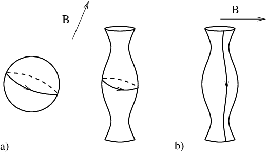
Figure 1: The Fermi surfaces containing only closed trajectories (a) and the Fermi surface containing open periodic trajectories at special directions of ${\bf B}$ (b).

We note here that the relations (8) and (9) should be understood only as asymptotic expressions and may contain additional dimensionless constants for each of the components $\,\sigma^{ik}\,$. We also use here the notation $\,*\,$ for arbitrary dimensionless constants of the order of unity.

It is easy to see that the main difference in the conductivity behavior in the cases considered above is the strong anisotropy of the conductivity in the plane, orthogonal to ${\bf B}$, observed in the second case. This property is a direct consequence of the special form of the corresponding electron trajectories and makes it possible to measure the mean direction of the periodic open trajectories in the $\,{\bf p}$-space.

In the works [54, 55], open trajectories of a more general type on Fermi surfaces of different shapes were considered. Let us say, that the trajectories, considered in [54, 55], are not periodic in general, but also have a mean direction in the plane orthogonal to ${\bf B}$. As a result, the conductivity behavior also exhibits strong anisotropic properties in strong magnetic fields in the presence of trajectories of this type on the Fermi surface. The works [51, 52, 53], as well as the book [50], provide a broad overview of the issues related to the electronic properties of metals, and in particular the issues related to transport phenomena in strong magnetic fields examined during that period. We would also like to give here a reference to the work [44] in which a return to this range of issues is made after a considerable time, and containing also aspects that arose in the later period.

As we have said above, the problem of the complete classification of possible types of trajectories of the system (7) was set by S.P. Novikov in the early 1980s and has now been studied with sufficient completeness, allowing to describe all essentially different types of open electron trajectories. In this chapter we will focus on the most significant physical results arising from the mathematical description of the trajectories of system (7), obtained in the recent decades.

As we noted in the previous chapter, the most significant part in the classification of open trajectories of system (7) is the description of stable open trajectories obtained in the works of A.V. Zorich and I.A. Dynnikov. We shall try to describe here the most interesting physical consequences arising when such trajectories appear on the Fermi surface.

Since the orbits of the solutions of (7) are the level sets of all siblings $\varepsilon_{\psi_{a}}$ of the quasiperiodic function in two variables with three quasiperiods $\varepsilon_{\psi}$, by Theorem 1 such trajectories always possess the following two remarkable properties:

1. Any stable open trajectory of system (7) in the $\,{\bf p}$-space lies in a straight strip of finite width in a plane $\psi_{a}$ (Fig. 2);

2. For a fixed direction ${\bf B}$, all stable open trajectories in the $\,{\bf p}$-space have the same mean direction, given by ${\bf B}\times\ell_{\varepsilon}({\bf B})$.

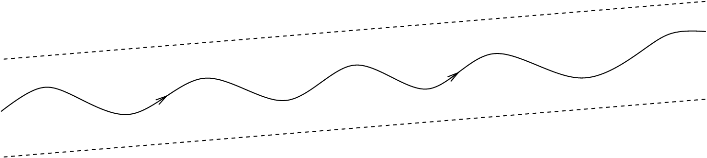
Figure 2: A stable open trajectory in the plane orthogonal to ${\bf B}$ in the $\,{\bf p}$-space.

As pointed out in [74], the presence of stable open trajectories on the Fermi surface always entails a strong anisotropy of the conductivity tensor in the plane, orthogonal to ${\bf B}$, in the limit $\,\omega_{B}\tau\,\rightarrow\,\infty\,$. Because of this, the topological quantum first integral $\ell_{\varepsilon}({\bf B})$ is observable experimentally. We call Stability Zones the sets ${\cal D}_{l,\varepsilon}$ defined by $\ell_{\varepsilon}({\bf B})=l$, so that for every ${\bf B}\in{\cal D}_{l,\varepsilon}$ all non-singular open orbits are strongly asymptotic to ${\bf B}\times l$.

Both the topological quantum first integral and the geometry of the Stability Zones contain important information about the electron spectrum in a crystal that is directly related to the determination of parameters of this spectrum in real materials. At the same time, both theoretical and experimental determination of the exact boundaries of the Stability Zones for a given dispersion relation represents a non-trivial problem that requires the use of rather special methods. As an example of a theoretical determination of the boundaries of the Stability Zones, we can cite the work [27], where such calculations were performed for a number of analytical dispersion relations that arise in real crystals. As can be seen from the work [27], an accurate calculation of the structure of the Stability Zones on the angular diagram requires the development of both rather serious topological and computational methods. We hope, on the other hand, that the methods used in [27] must be applicable to a large number of different examples of complex Fermi surfaces and will prove extremely useful in determination the parameters of the dispersion relations in real materials. It must also be said that the experimental determination of the structure of the Stability Zones in real materials also presents a special problem because of a rather complicated analytical behavior of conductivity near their boundaries (see, e.g. [59]). In particular, the exact experimental determination of the mathematical boundaries of the Stability Zones also requires, in addition to direct study of conductivity, special experimental techniques ([60]).

Another very important achievement of mathematical research of the S.P. Novikov problem was the discovery of new, previously unknown, types of trajectories of system (7), which have very complicated (chaotic) behavior. The first trajectories of this type were constructed at the beginning of Nineties by S.P. Tsarev for “partially irrational” directions of ${\bf B}$ and have an obvious chaotic behavior on the Fermi surface. At the same time, the behavior of the Tsarev trajectories in planes orthogonal to ${\bf B}$ resembles the behavior of stable open trajectories, in particular, they all have asymptotic directions in these planes (although they do not lie in straight strips of finite width). As a result, the behavior of the conductivity tensor in the presence of the Tsarev trajectories on the Fermi surface is also very similar to its behavior in the presence of stable open trajectories, in particular, it has a strong anisotropy in this case. As already mentioned, trajectories of Tsarev type can appear only for directions of the magnetic field of irrationality 2 (the plane orthogonal to ${\bf B}$ contains a reciprocal lattice vector) and it can be shown (see [36]) that all chaotic trajectories arising for such directions of ${\bf B}$ have the properties described above.

The first examples of chaotic trajectories for directions of ${\bf B}$ of maximal irrationality were constructed by I.A. Dynnikov in the work [36]. Trajectories of this type have a strongly chaotic behavior both on the Fermi surface and in planes orthogonal to ${\bf B}$ (Fig. 3). As can be seen, the behavior of a Dynnikov trajectory in a plane orthogonal to ${\bf B}$ resembles in a certain sense the diffusion motion, which leads to the most complicated dependence of the conductivity on the value of $\,B\,$.

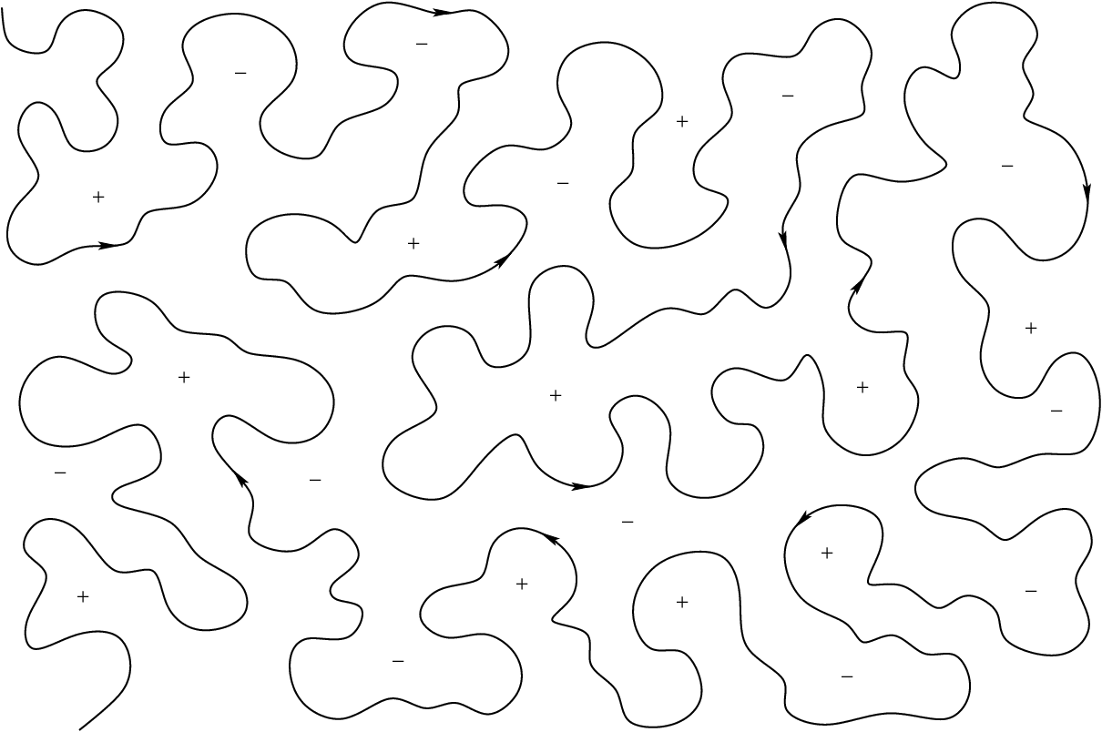
Figure 3: The geometry of the Dynnikov chaotic trajectory in the plane orthogonal to $\,{\bf B}$.

The most interesting moment in the behavior of conductivity in the presence of the Dynnikov trajectories is the blocking of the conductivity along the direction of ${\bf B}$ in strong magnetic fields ([57]), such that the entire Fermi surface area covered by the corresponding chaotic trajectories does not contribute to the conductivity along ${\bf B}$ in the limit $\,\omega_{B}\tau\,\rightarrow\,\infty\,$. As a result, for the corresponding directions on the angular diagram, rather sharp minima in conductivity along the direction of ${\bf B}$ should be observed in strong magnetic fields.

Another interesting feature of the conductivity behavior in the presence of the Dynnikov trajectories on the Fermi surface is the appearance of fractional powers of the parameter $\,\omega_{B}\tau\,$ in the dependence of the components of the conductivity tensor on the value of the magnetic field ([57]). It must be said that the analysis carried out for equation (5) in the presence of such trajectories actually used in this case an additional property (self-similarity) of trajectories constructed in [36], which, generally speaking, is not observed in the general case for Dynnikov chaotic trajectories. Quite recently, however, it was possible to show that the appearance of fractional powers of a parameter $\,\omega_{B}\tau\,$ in the conductivity behavior in the presence of trajectories of this type is actually a common fact and is connected with the existence of the so-called Zorich - Kontsevich - Forni indices (see [86, 87, 88, 82, 89, 83]) describing the behavior of such trajectories on a large scale ([65]).

As mentioned in the previous section, the general properties of chaotic trajectories of Dynnikov type, as well as the properties of the set of directions of ${\bf B}$ at which such trajectories can be observed, are the subject of the most active research at the present time. Let us also note here that, in spite of the fact that Dynnikov chaotic trajectories are not trajectories of general position, they may nevertheless be typical for Fermi surfaces of a certain type (see [61]).

Let us say, that, in addition to describing the new quantities and the new regimes observed in conductivity studies, a mathematical investigation of the Novikov problem actually made it possible to construct a complete classification of the possible types of conductivity behavior in strong magnetic fields, including all cases of both generic and non-generic position. Here we only point out that the most detailed mathematical consideration of the various situations possible for system (7) is presented in the work [37]. We also note that a detailed exposition of the physical consequences of the classification obtained can be found in the works [73, 62, 63].

We would also like to describe here another application of the Novikov problem related to transport phenomena in two-dimensional electron systems in a magnetic field, placed in an artificially created potential in the plane of the system.

It is well known that two-dimensional electron systems are of great interest from the point of view of modern experimental and theoretical physics in connection with their very different applications in various fields. A special class of such systems are systems in an external magnetic field, which can be either parallel or perpendicular to the plane of the system. We will consider here systems in a perpendicular magnetic field, placed in a quasiperiodic plane potential, which can be created using a variety of techniques.

We will be interested in the case when the behavior of electrons in a magnetic field can be described in the semiclassical approximation. In this case, we can imagine electrons moving along cyclotron orbits, the centers of which experience a slow drift under the influence of external fields (Fig. 4). As an external field, we will consider a special external potential $\,V({\bf x})\,$ having quasiperiodic properties, which can also be considered as a model of a pseudo-random potential in the plane. We note here that many techniques for creating such potentials presuppose in reality the use of a superposition of periodic potentials with different periods (in the plane). It is easy to see that such techniques make it possible to obtain quasiperiodic potentials with any number of quasiperiods, which makes the problem under consideration quite relevant for such systems.

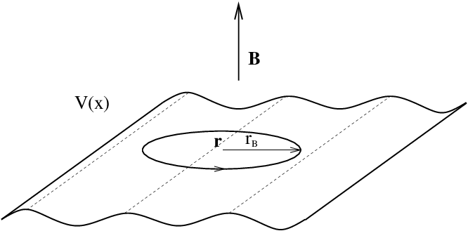
Figure 4: The cyclotron electron orbit in the potential $\,V({\bf x})\,$.

As it can be established (see e.g. [42, 14]), in the main order of the adiabatic approximation the centers of cyclotron orbits must drift along the level lines of a certain modified potential $\,{\bar{V}}({\bf x})\,$, obtained from the potential $\,V({\bf x})\,$ by averaging over the corresponding cyclotron electron orbits. It is also easy to see that the potential $\,{\bar{V}}({\bf x})\,$ has the same quasiperiodic properties as the potential $\,V({\bf x})\,$. As in the case of normal metals, the motion of electrons along the cyclotron orbits, as well as the drift of the cyclotron orbits in the potential, does not change the equilibrium statistical distribution of electrons in the two-dimensional system. At the same time, the peculiarities of the motion of the orbits along the level lines of the potential $\,{\bar{V}}({\bf x})\,$ have a significant effect on electronic transport phenomena that arise, say, in an electric field (electrical conductivity), or in the presence of a temperature gradient (thermal conductivity). As a result, the description of the geometry of the level lines of a quasiperiodic potential $\,{\bar{V}}({\bf x})\,$ has the same significance in this problem as for electron transport phenomena in metals.

As we have seen above, the problem of the geometry of the level lines of quasiperiodic potentials on the plane can be considered at present solved for the case of three quasiperiods. In particular, we can also transfer here all the results concerning the description of electron transport phenomena determined by the geometry of the level lines of the potential $\,{\bar{V}}({\bf x})\,$. We note here that, unlike the case of normal metals, practically all the parameters of the problem are controlled in the described systems, so here it is possible to obtain any of the conductivity regimes described earlier. In particular, by changing the parameters of the potential, as well as the concentration of electrons in the system, we can easily achieve a regime of suppression of conductivity in the system (closed level lines), anisotropic conductivity regime (stable open level lines), or more complex regimes of diffuse conductivity (chaotic level lines).

Among the cases with a larger number of quasiperiods, we should especially point the case of four quasiperiods, where deep topological results about regular level lines have now been obtained ([70, 72]). As for cases with five or more quasiperiods, at the moment the most probable is the prevalence here of complex chaotic regimes of behavior of the level lines of the corresponding potentials.

4 Experimental and numerical study of level sets of QP functions on $\mathbb{R}^{2}$ with 3 quasiperiods

No algorithm is known to write an analytical or approximate perturbative expression of the set ${\cal D}_{F}$ and of the functions $l_{F},u_{F}$ relative to a general function $F\in C^{\infty}({\mathbb{T}}^{3})$. In fact, an analytical description for non-trivial ${\cal D}_{F}$ and $\ell_{F}$ has been found only in case of a very simple piecewise linear function [30]. Numerical methods are therefore necessary in order to get some intuition on the nature of such sets and maps and in order to predict theoretically from first principles the physical behavior of systems involving QP functions.

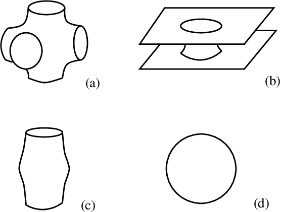
Figure 5: Examples of surfaces embedded in ${\mathbb{T}}^{3}$ with rank respectively 3,2,1,0.

In order to illustrate the numerical algorithm we used so far to explore this problem we need first to describe its extrinsic geometry (e.g. see [69]). In particular, rather than considering the foliation induced on a plane $\psi:\mathbb{R}^{2}\to\mathbb{R}^{3}$ by the level sets of a periodic function $F$, we focus instead on the foliation induced on a triply periodic surface $F_{c}=\{F=c\}\subset{\mathbb{T}}^{3}$ by the bundle of (projections into ${\mathbb{T}}^{3}$ of) planes of all siblings of $\psi$.

In the generic case, $\psi$ is fully irrational and so the planar sections by the $\psi_{a}$ will cut $F_{c}$ in some finite number of open cylinders $C_{i}$ foliated by compact orbits and some finite number of closed components $N_{j}$ equal to the closure of any open orbits in it. Each of these $N_{j}$ has a boundary which is the union of finitely many loops homotopic to zero, all of them lower or upper bases of some of the cylinders $C_{i}$. Since all the boundary components are homotopic to zero, it makes sense to define the genus of the $N_{j}$ as the genus of the surfaces without boundary $\tilde{N}_{j}$ obtained from the corresponding $N_{j}$ quotienting to a single point.

Definition 4.

Given a surface $M_{g}$ of genus $g$ and an embedding $i:M_{g}\to{\mathbb{T}}^{3}$, we call rank of the embedding the rank of the induced ring homomorphism $i_{*}:H_{1}(M_{g},\mathbb{Z})\simeq\mathbb{Z}^{2g}\to H_{1}({\mathbb{T}}^{3},\mathbb{Z})\simeq\mathbb{Z}^{3}$.

Intuitively, if $M_{g}$ is embedded with rank $r$ then $\pi^{-1}(M_{g})$ lies inside a finite-width neighborhood of a $r$-dimensional linear subspace of $\mathbb{R}^{3}$. In particular, no open orbits can arise for generic $\psi$ when $r=0,1$ and the problem is trivial when $r=2$, so we will assume from now on that $r=3$ (e.g. see Fig. 5). Two fundamental observation in elementary topology pointed out by Dynnikov lead to the definition of $\ell_{F}$, namely:

Theorem 5 (Dynnikov [35]).

If a component $N_{j}$ contains an orbit whose counterimage in the universal covering is strongly asymptotic to a straight line, then $\tilde{N}_{j}$ must have genus 1 and must be embedded in ${\mathbb{T}}^{3}$ with rank 2, namely $[\tilde{N}_{j}]$ is an indivisible integer 2-cycle in $H_{2}({\mathbb{T}}^{3},\mathbb{Z})\simeq\mathbb{Z}^{3}$. Moreover, in this case for all other components $N_{j^{\prime}}$ of $F_{c}$ and of any other level surface $F_{c^{\prime}}$ hold same properties and all of them represent, modulo sign, the same 2-cycle ${\bf l}=[\tilde{N}_{j}]$.

Equivalently, by filling up with planar discs all holes of the counterimage of any one of these components in the universal covering we get a warped plane, namely an embedding $\mathbb{R}^{2}\to\mathbb{R}^{3}$ whose image lies in a finite-width region between two planes perpendicular to ${\bf l}$ (thought as a direction in $\mathbb{R}^{3}$). This integral direction ${\bf l}$ is indeed the value of $\ell_{F}$ at ${\bf B}_{\psi}$.

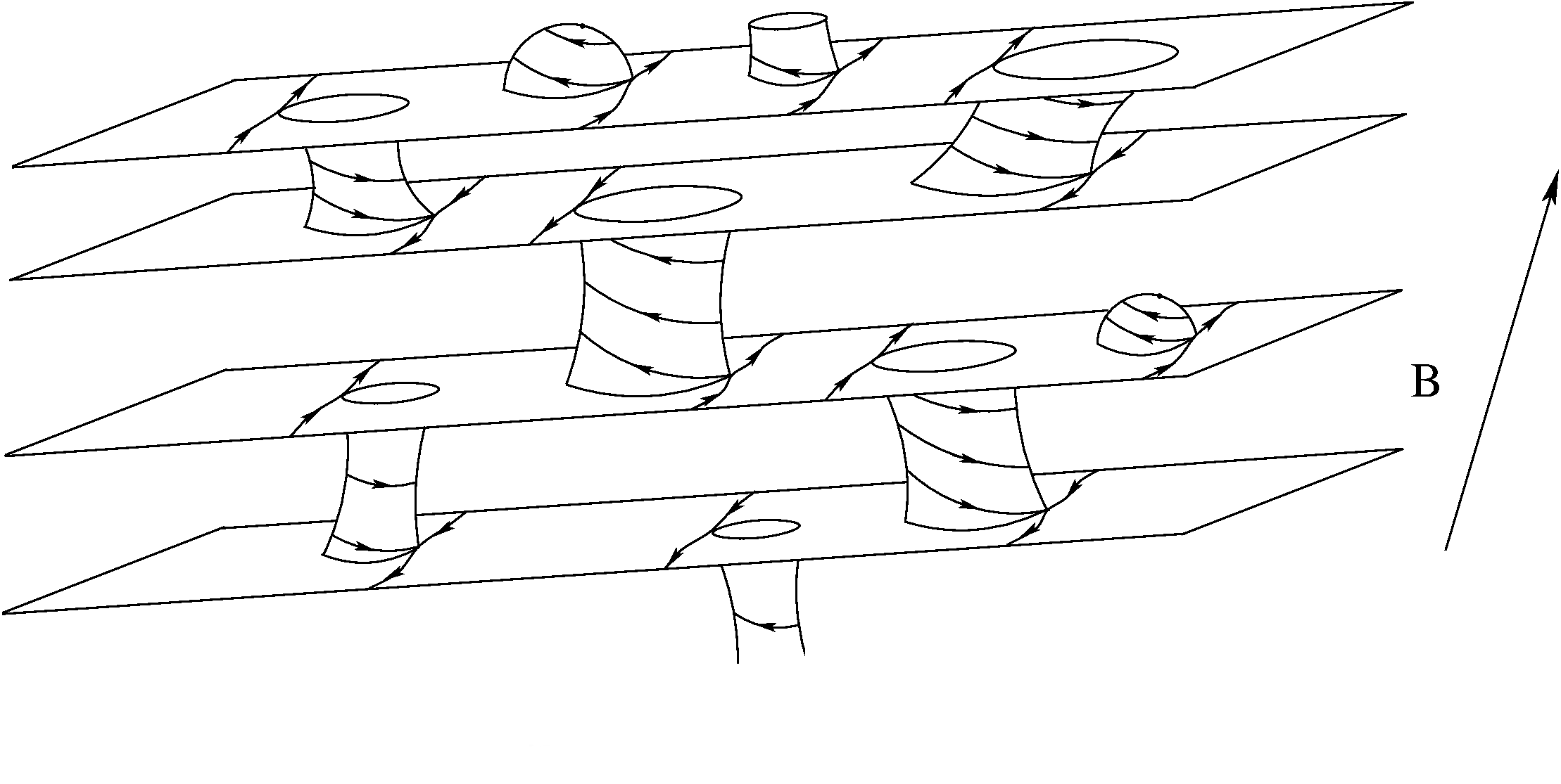
Figure 6: Typical structure of the sections of a periodic surface by a bundle of parallel planes: in this case the surface gets subdivided into four $N_{j}$ components ( warped planes) filled by open orbits, six cylinders filled by closed orbits and a few caps also filled by closed orbits.

Recall that in the homology of a manifold $N^{n}$ it is defined an intersection product $\cap:H_{i}(N^{n})\times H_{n-j}(N^{n})\to\mathbb{Z}$ defined so that $[a]\cap[b]$ is the signed number of intersection of any two representatives of the cycles $a$ and $b$ transversal to each other. Since two leaves of the same foliation cannot intersect each other, the non-trivial loops contained in every genus-1 rank-2 component of $M_{g}$ do not intersect any of the trivial (in ${\mathbb{T}}^{3}$) loops in the cylinders $C_{i}$. In order to find $\ell_{F}({\bf B}_{\psi})$, therefore, it is enough to find the rank-2 sublattice of $H_{1}({\mathbb{T}}^{3},\mathbb{Z})$ of all 1-cycles such that their homology intersection product with $\ell_{F}({\bf B}_{\psi})$ is 0. This can be accomplished by selecting a canonical basis $\{e_{i},f_{j}\}$ of $H_{1}(M_{g},\mathbb{Z})$, namely so that $e_{i}\cap f_{j}=\delta_{ij}$, evaluating the homology classes $c_{i}$ corresponding to each cylinder of compact orbits and finding the symplectic orthogonal of the span of the $c_{i}$, namely the sublattice $K\subset H_{1}(M_{g},\mathbb{Z})$ of the homology classes whose intersection product with all $c_{i}$ is zero. The push-forward $i_{*}K\subset H_{1}({\mathbb{T}}^{3},\mathbb{Z})$ is the rank-2 sublattice we were looking for.

The first (semi-analytic) study of a concrete case of QP function was done by Dynnikov [35] for

$${\mathfrak{c}}(x,y,z)=\cos(2\pi x)+\cos(2\pi y)+\cos(2\pi z)\,.$$

The level sets ${\mathfrak{c}}_{c}$ have genus 3 and rank 3 for $c\in(-1,1)$ and genus 0 and rank 0 otherwise. The function ${\mathfrak{c}}$ satisfies the property $T^{*}F=-F$, where $T$ is the translation by $1/2$ in the three coordinate directions, so that when $\psi_{a}^{*}{\mathfrak{c}}=c$ has an open level set then also $\psi_{a}^{*}{\mathfrak{c}}=-c$ has, meaning ultimately that $l_{{\mathfrak{c}}}=-u_{{\mathfrak{c}}}$ and so that, in particular, in order to study ${\cal D}_{\mathfrak{c}}$ it is enough looking at the level ${\mathfrak{c}}_{0}$. Dynnikov was able to find the analytical expression for the 10 largest connected components of ${\cal D}_{\mathfrak{c}}$ and their corresponding value of $\ell_{\mathfrak{c}}$.

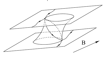
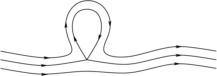
Figure 7: (left) A typical critical section for a direction of the magnetic field at the boundary of a stability zone: the upper and lower bases of a cylinder of closed orbits collapse on each other creating a saddle connection. (right) A critical saddle point and behavior of trajectories near it.

The idea of this method is the following. Note first that, since $c_{0}$ has genus 3 and its curvature is strictly negative (except for eight points where it is zero), all critical points, namely points where ${\bf B}$ is perpendicular to the surface, are of saddle type (see Fig. 7). Because of the Poincaré-Hopf index theorem, the sum of the indices of a generic vector field on a manifold must equal its Euler characteristics and so a generic (rational or irrational) direction ${\bf B}\in{\mathbb{R}{\mathrm{P}}^{2}}$ must have exactly four of them: $4\cdot(-1)=2-2\cdot 3$. When ${\bf B}\in{\mathbb{Q}{\mathrm{P}}^{2}}$ (that’s the only case we can deal with numerically!), generically each of these four saddle critical points is fully closed, namely the four tails are pairwise connected to each other forming two loops in such a way that one of the loops is homotopic to zero while the second is not.

The four loops homotopic to zero are the bases of the two cylinders of closed orbits – recall that ${\mathbb{Q}{\mathrm{P}}^{2}}\subset{\cal D}_{\mathfrak{c}}$, so the open orbits induced by ${\bf B}$ are strongly asymptotic to a straight line and so the surface for each such direction is decomposed into a pair of components $N_{1},N_{2}$ and a pair of cylinders $C_{1},C_{2}$ (see Fig. 6). Let $p_{1}\in\mathbb{R}^{3}$ be one of the critical points. One can numerically find, by trial and error, the coordinates of the critical point $p_{2}$ in $\mathbb{R}^{3}$ at the opposite base of the cylinder. Clearly, in order for a new decomposition of ${\mathfrak{c}}_{0}$ in cylinders and warped planes to arise it is necessary for the former cylinders to collapse to zero height (see Fig. 7), so the equation $\langle p_{1}-p_{2},{\bf B}\rangle=0$ defines a segment of the boundary of the stability zone where the original ${\bf B}$ lies. By following (numerically) the evolution of the zero-height cylinders, at a certain point a second pair of critical points appears and the cylinders will undergo a surgery. These points are vertices of the stability zones. By following the lines and vertices defined by the new pairs until we get back to the starting side, one ends up with the entire analytical boundary of a stability zone.

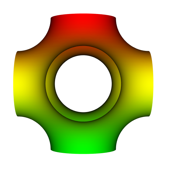
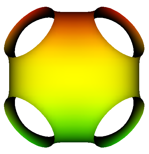
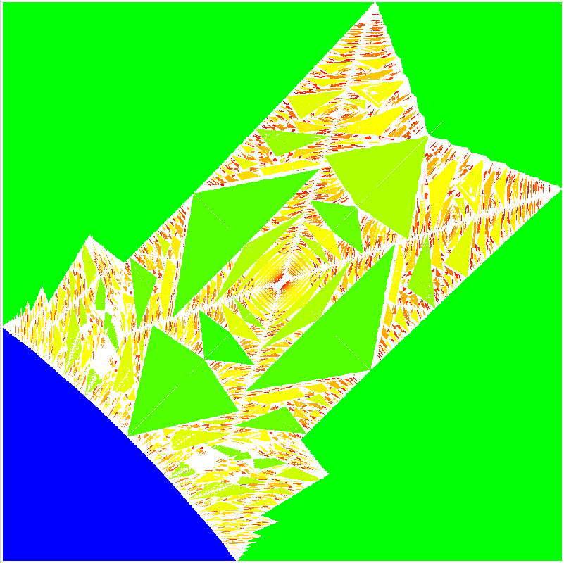
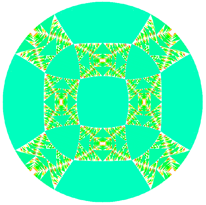
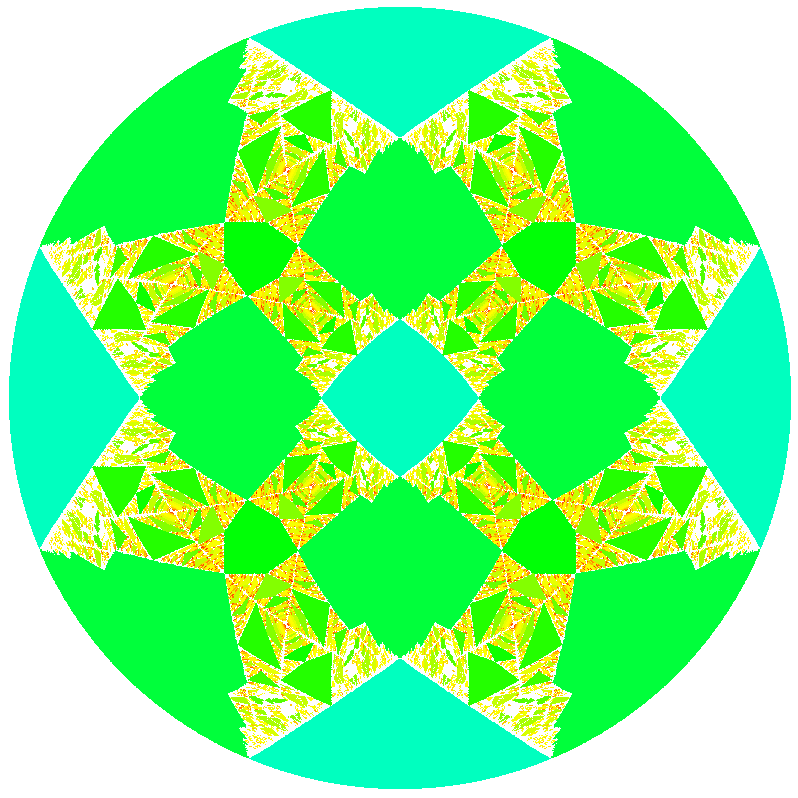
Figure 8: (left) From top to bottom: the surface ${\mathfrak{c}}_{0}$, the SM ${\cal D}({\mathfrak{c}})$ in the square $[0,1]^{2}$ of the chart $B_{z}=1$ and in the whole ${\mathbb{R}{\mathrm{P}}^{2}}$. (right) From top to bottom: the surface ${\mathfrak{d}}_{0}$, the SM ${\cal D}({\mathfrak{d}})$ in the square $[0,1]^{2}$ of the chart $B_{z}=1$ and in the whole ${\mathbb{R}{\mathrm{P}}^{2}}$.

The drawback of this method is that it does not look suitable to be implemented into a programming language. In order to bypass this problem, the first author implemented the algorithm to evaluate $\ell_{\mathfrak{c}}({\bf B})$ in the open source C++ library NTC [22]. NTC is built on top of the open source C++ library VTK by W. Schroeder, K. Martin and B. Lorense [77], one of the most popular computational geometry library available online in the last two decades. VTK implements fundamental geometry operations such as generating, within some cuboid, the mesh for the level set of a given function or generating the mesh of the intersection between two such surfaces within some fixed cuboid.

While restricting an unbounded set to a bounded cuboid causes in general a big loss of information, it is not so for a periodic set since the whole information about it is contained inside a basic cell. Surprisingly enough, in the authors’ knowledge, none of the general-purpose computational geometry libraries available online implement special algorithm for periodic geometry, although that is the only geometry where, quite remarkably, “it is possible to keep infinity inside a bounded box”. The NTC library implements exactly all periodic geometry algorithms described above to evaluate $\ell_{\mathfrak{c}}({\bf B})$: finding the critical points induced by ${\bf B}$ on ${\mathfrak{c}}$; retrieving the (whole) intersection (in ${\mathbb{T}}^{3}$) between an embedded 2-torus passing and a (periodic) surface; evaluating the homology of loops in $H_{1}({\mathfrak{c}},\mathbb{Z})$ and in $H_{1}({\mathbb{T}}^{3},\mathbb{Z})$; finding the homology class in ${\mathbb{T}}^{3}$ of a loop with a given homology class in ${\mathfrak{c}}$. In order to get an approximation for ${\cal D}_{\mathfrak{c}}$ and $\ell_{\mathfrak{c}}$ with NTC it is enough to fix a grid in ${\mathbb{Q}{\mathrm{P}}^{2}}$ and evaluate $\ell_{\mathfrak{c}}$ at all elements of the grid.

NTC currently supports functions with level surfaces of genus $g=3$ and $g=4$. The first is the simplest case with a non-trivial set ${\cal D}_{\mathfrak{c}}$, the second is the case of the Fermi surfaces of the noble metals Copper, Gold and Silver. In Fig. 8 (left) we show ${\mathfrak{c}}_{0}$, the whole SM ${\cal D}({\mathfrak{c}})$ and a detail of it in the region $[0,1]^{2}$ in the chart $B_{z}=1$. A rough numerical evaluation of its box dimension gives an estimate of about 1.83, in agreement with Novikov’s Conjecture 1. In Fig. 8 (right) we show the set ${\cal D}_{\mathfrak{d}}$ for the map

$${\mathfrak{d}}(x,y,z)=\cos(2\pi x)\cos(2\pi y)+\cos(2\pi y)\cos(2\pi z)+\cos(2\pi z)\cos(2\pi x)\,,$$

whose regular level sets ${\mathfrak{d}}_{c}$ are either spheres (for $c<-1$ and $c>0$) or genus-4 surfaces (for $-1<c<0$). Each of the genus-4 level sets has topological rank 4. Note also that ${\mathfrak{d}}$, besides being invariant by integer translations along the coordinate axes, is invariant with respect to translations by $1/2$ along the cube diagonals, namely it has a bcc invariance. A rough numerical evaluation of its box dimension of about 1.69, again in agreement with Novikov’s Conjecture 1. A striking confirmation of the correctness of these numerical data is shown in [30]. In that article it is discussed the case of a simple piecewise linear function $F$ where the first author and Dynnikov were able to find an analytical expression for $\ell_{F}$; the numerical data for that case agrees at 100% level with the analytical ones.

We switch now to the experimental data. As mentioned in the previous sections, according to the semiclassical approximation the topology of the level sets of the QP function $\varepsilon_{\psi}$ given by the restriction of the Fermi energy function to some plane $\psi$ perpendicular to ${\bf B}$ dictates the asymptotic behavior of the magnetoresistance for $\|{\bf B}\|\to\infty$ and so it can be detected experimentally. Starting from the end of Fifties, stereographic maps were experimentally obtained for many metals, mostly by Pippard, Alekseevskii and Gaidukov [76, 2, 43, 3, 8, 4, 5, 6, 7, 9]. The maps for Gold, Silver and Copper are shown, respectively from top to bottom, in the middle column of Fig. 9. In these stereographic maps, ${\mathbb{R}{\mathrm{P}}^{2}}$ is represented as a disc and regions are shaded for those directions of the magnetic field open orbits are detected and left blank otherwise. Mathematically, this corresponds to the fact that we look only at a single level set $\varepsilon_{\psi}=c$, the Fermi energy level, for every sibling of $\psi$ and, correspondingly, we define a reduced map $\ell_{\varepsilon,c}({\bf B})$ that, for any ${\bf B}\in{\cal D}_{\varepsilon}$, is equal to $\ell_{\varepsilon}({\bf B})$ if $c\in[l_{\varepsilon},u_{\varepsilon}]$ and to $(0,0,0)$ (meaning absence of open orbits) otherwise. We denote by ${\cal D}_{\varepsilon,c}$ the subset of ${\cal D}_{\varepsilon}$ where $\ell_{\varepsilon,c}({\bf B})\neq(0,0,0)$.

No comparison of these experimental data with theoretical prediction was possible for about half a century because of the lack of knowledge about the levels of QP functions. In the right column of Fig. 9 we show the numerical approximations of the sets ${\cal D}_{\varepsilon,c}$ relative to approximated expressions of the Fermi surfaces retrieved from the physics literature. Note that a strong magnetic field (of the order of 10 Tesla) is needed in order for this phenomenon to become visible and these old experimental data was taken right at the threshold (with magnetic fields of about 1 Tesla). Similarly, the trigonometric approximations we used for the Fermi energy functions is far from being the best approximation available to date (but it was the simplest and quickest to implement in the NTC library). Yet, the match between experimental data and theoretical prediction is remarkably high (see Fig. 9).

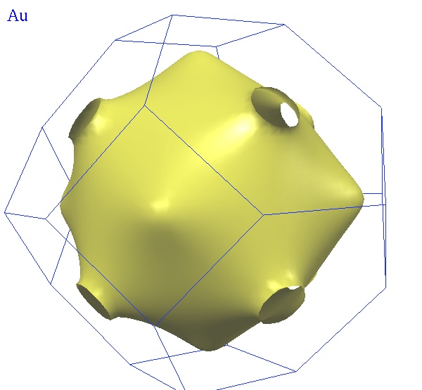
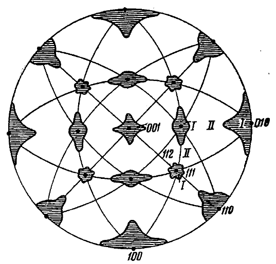
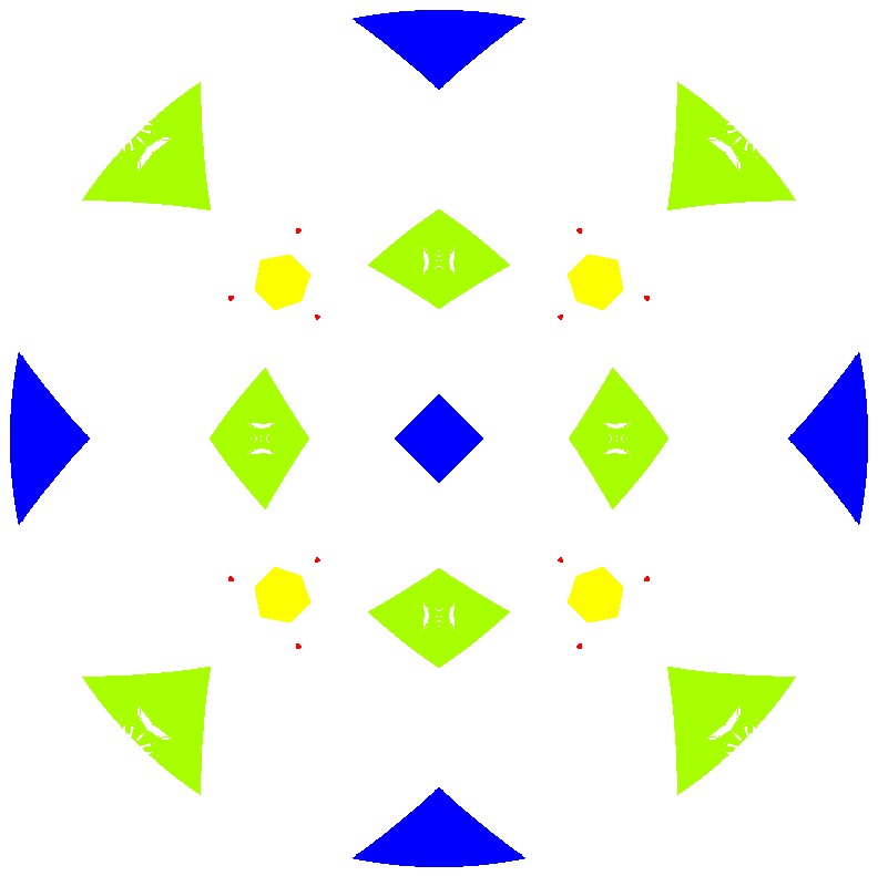
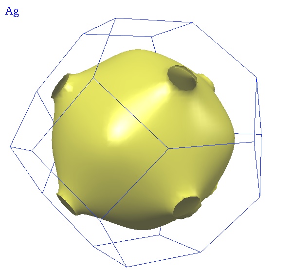
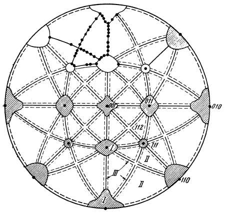
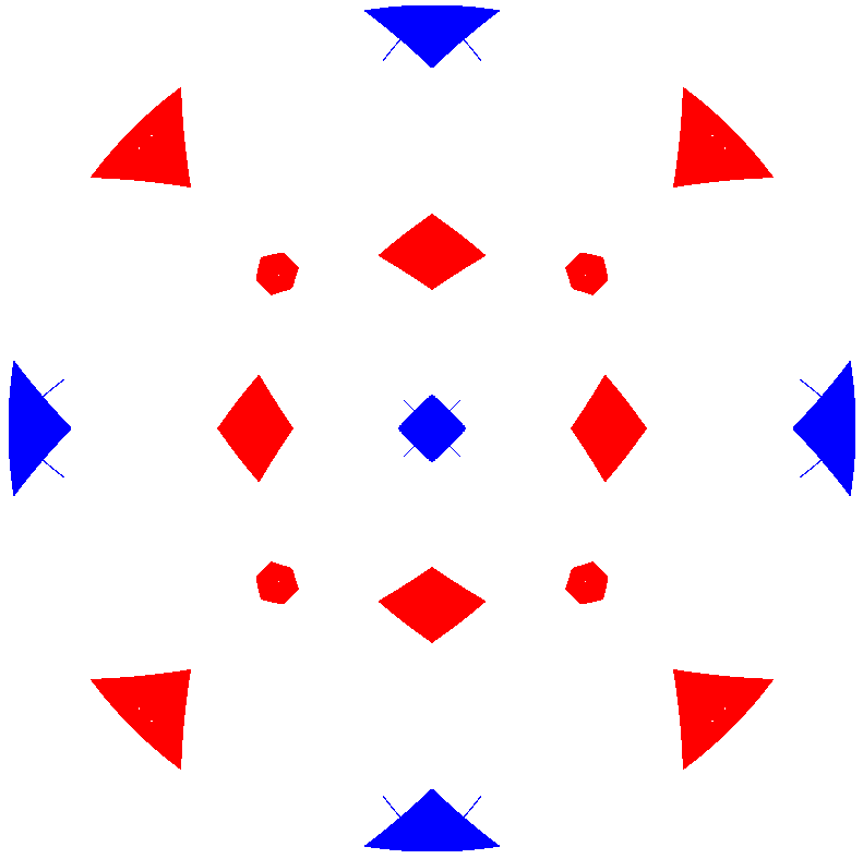
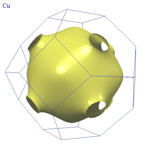
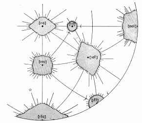
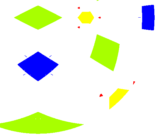
Figure 9: (top) FS of Gold and its experimental [43] and numerical [26, 27] Stereographic Map. (middle) FS of Silver and its experimental [5] and numerical [26, 27] Stereographic Map. (bottom) FS of Copper and its experimental [46] and numerical Stereographic Map.

We point out that the reason for using such old experimental data is that, after about a decade of great excitement that saw a large number of theoretical and experimental articles dedicated to the subject, the interest of the solid state community in the topic decreased a lot, possible exactly because no way was found to reproduce the experimental data from first principles, and so in our knowledge no new stereographic maps were produced since the Sixties. Recently, though, some new experimental result, in particular on the role of dislocations in the deformation of the map $\ell_{\varepsilon,c}$ for Copper, has been published by M. Niewczas and his student Q. Bian [16, 17], giving some hope for the appearance of accurate stereographic maps in a near future. Now that we have the possibility, it would be indeed extremely interesting to have some more reliable experimental data to compare to.

There are quite a few important advances to still make in this field:

• Extend NTC in order to make it work with surfaces of genus 7 (so is the Fermi surface of Lead [4]).

• Implement some algorithm in NTC able to produce accurate approximations of Fermi surfaces.

• Explore sets ${\cal D}_{\varepsilon}$ and ${\cal D}_{\varepsilon,c}$ for several other triply periodic functions with level surfaces of genus 7 or less.

• Optimize NTC to make it faster and more accurate.

• Start the study the case of 4 and 5 quasiperiods.

Funding

This material is based upon work supported by the National Science Foundation under Grant No. DMS-1832126 and the project “Dynamics of complex systems” (L.D. Landau Institute for Theoretical Physics).

References

- [1] A.A. Abrikosov. Fundamentals of the Theory of Metals. North Holland, 1988.
- [2] N.E. Alexeevskii and Yu.P. Gaidukov. Measurement of the electrical resistance of metals in a magnetic field as a method of investigating the Fermi surface. JETP, 9:311, 1959.
- [3] N.E. Alexeevskii and Yu.P. Gaidukov. The anysotropy of magnetoresistance and the topology of Fermi Surfaces of metals. JETP, 10:481, 1960.
- [4] N.E. Alexeevskii and Yu.P. Gaidukov. The Fermi surface of Lead. JETP, 14:2:256, 1961.
- [5] N.E. Alexeevskii and Yu.P. Gaidukov. Concerning the Fermi surface of Tin. JETP, 14:770, 1962.
- [6] N.E. Alexeevskii and Yu.P. Gaidukov. Fermi surface of Silver. JETP, 15:49, 1962.
- [7] N.E. Alexeevskii and Yu.P. Gaidukov. Open cross sections of Cadmium, Zinc and Thallium Fermi Surfaces. JETP, 16:1481, 1963.
- [8] N.E. Alexeevskii, Yu.P. Gaidukov, I.M. Lifschitz, and V.G. Peschanskii. The Fermi Surface of Tin. JETP, 12:837, 1961.
- [9] N.E. Alexeevskii, E. Karstens, and V.V. Mozhaev. Investigation of the galvanometric properties of Pd. JETP, 19:1979, 1964.
- [10] V.I. Arnold. Huygens and Barrow, Newton and Hooke: pioneers in mathematical analysis and catastrophe theory from evolvents to quasicrystals. Springer Science & Business Media, 1990.
- [11] V.I. Arnold and A.B. Givental. Symplectic Geometry, in Dynamical Systems IV, Encyclopaedia of Mathematical Sciences, ed. by VI Arnold and SP Novikov, 1990.
- [12] A. Avila, P. Hubert, and A. Skripchenko. Diffusion for chaotic plane sections of 3-periodic surfaces. Inventiones mathematicae, 206(1):109–146, 2016.
- [13] A. Avila, P. Hubert, and A. Skripchenko. On the Hausdorff dimension of the Rauzy gasket. Bulletin de la société mathématique de France, 144(3):539–568, 2016.
- [14] C.W.J. Beenakker. Guiding-center-drift resonance in a periodically modulated two-dimensional electron gas. Physical Review Letters, 62(17):2020, 1989.
- [15] A.S. Besicovitch. On generalized almost periodic functions. Proceedings of the London Mathematical Society, 2(1):495–512, 1926.
- [16] Q. Bian. Magnetoresistance and Fermi Surface of Copper Single Crystals Containing Dislocations. PhD thesis, 2010. http://hdl.handle.net/11375/18932.
- [17] Q. Bian and M. Niewczas. Theory of magnetoresistance due to lattice dislocations in face-centred cubic metals. Philosophical Magazine, 96(17):1832–1860, 2016.
- [18] S. Bochner. Beiträge zur theorie der fastperiodischen funktionen I. Mathematische Annalen, 96(1):119–147, 1927.
- [19] S. Bochner. Beiträge zur theorie der fastperiodischen funktionen II. Mathematische Annalen, 96(1):383–409, 1927.
- [20] P.P.F. Bohl. Ueber die darstellung von Functionen einer variabeln durch trigonometrische reihen mit mehreren einer variabeln Proportionalen argumenten… Druck von C. Mattiesen, 1893.
- [21] H. Bohr. Zur theorie der fastperiodischen funktionen. Acta Mathematica, 47(3):237–281, 1926.
- [22] R. De Leo. NTC: GNU NTC library, 1999–2018.
- [23] R. De Leo. The existence and measure of ergodic foliations in Novikov’s problem of the semiclassical motion of an electron. Russian Mathematical Surveys, 55:166–168, 2000.
- [24] R. De Leo. Numerical analysis of the Novikov problem of a normal metal in a strong magnetic field. SIADS, 2(4):517–545, 2003.
- [25] R. De Leo. Characterization of the set of “ergodic directions” in the Novikov problem of quasi-electrons orbits in normal metals. Russian Mathematical Surveys, 58(5):1042–1043, 2004.
- [26] R. De Leo. Topological effects in the magnetoresistance of Au and Ag. Physics Letters A, 332:469–474, 2004.
- [27] R. De Leo. First-principles generation of Stereographic Maps for high-field magnetoresistance in normal metals: an application to Au and Ag. Physica B, 362:62–75, 2005.
- [28] R. De Leo. Proof of a Dynnikov conjecture on the Novikov problem of plane sections of periodic surfaces. RMS, 60(3):566–567, 2005.
- [29] R. De Leo. Topology of plane sections of periodic polyhedra with an application to the truncated octahedron. Experimental Mathematics, 15:109–124, 2006.
- [30] R. De Leo and I.A. Dynnikov. Geometry of plane sections of the infinite regular skew polyhedron . Geometriae Dedicata, 138(1):51–67, 2009.
- [31] B.A. Dubrovin, I.M. Krichever, and S.P. Novikov. Integrable systems I, in Dynamical Systems IV, Encyclopedia of Mathematical Sciences, ed. by Arnold and SP Novikov, 1990.
- [32] B.A. Dubrovin, V.B. Matveev, and S.P. Novikov. Non-linear equations of Korteweg-de Vries type, finite-zone linear operators, and abelian varieties. Russian Mathematical Surveys, 31(1):59–146, 1976.
- [33] B.A. Dubrovin and S.P. Novikov. Periodic and conditionally periodic analogs of the many-soliton solutions of the Korteweg-de Vries equation. Zh. Eksper. Teoret. Fiz, 67(6):2131–2144, 1974.
- [34] I.A. Dynnikov. Proof of S.P. Novikov conjecture on the semiclassical motion of an electron. Usp. Mat. Nauk (RMS), 57:3:172, 1992.
- [35] I.A. Dynnikov. Surfaces in 3-torus: geometry of plane sections. Proc. of ECM2, BuDA, 1996.
- [36] I.A. Dynnikov. Semiclassical motion of the electron. A proof of the Novikov conjecture in general position and counterexamples. AMS Transl, 179:45–73, 1997.
- [37] I.A. Dynnikov. The geometry of stability regions in Novikov’s problem on the semiclassical motion of an electron. RMS, 54:1:21–60, 1999.
- [38] I.A. Dynnikov. Interval identification systems and plane sections of 3-periodic surfaces. Proceedings of the Steklov Institute of Mathematics, 263(1):65–77, 2008.
- [39] I.A. Dynnikov and S.P. Novikov. Topology of quasiperiodic functions on the plane. Russ. Math. Surv., 60(1):1–26, 2005.
- [40] I.A. Dynnikov and A. Skripchenko. Symmetric band complexes of thin type and chaotic sections which are not quite chaotic. Transactions of the Moscow Mathematical Society, 76:251–269, 2015.
- [41] E. Esclangon. Les fonctions quasi-périodiques… Gauthier-Villars, 1904.
- [42] H.A. Fertig. Semiclassical description of a two-dimensional electron in a strong magnetic field and an external potential. Phys. Rev. B, 38:996–1015, 1988.
- [43] Yu.P. Gaidukov. Topology of the Fermi surface for Gold. JETP, 10(5):913, 1960.
- [44] A.M. Kaganov and V.G. Peschanskii. Physics Reports, 372:445–487, 2002.
- [45] C. Kittel. Quantum Theory of Solids. Wiley, 1963.
- [46] J.R. Klauder, W.A. Reed, G.F. Brennert, and J.E. Kunzler. Study of the fine structure in the high-field galvanomagnetic properties and the Fermi Surface of Copper. Physical Review, 141(2):592, 1966.
- [47] Q.T. Le Tu, S.A. Piunikhin, and V.A. Sadov. The geometry of quasicrystals. Russian Mathematical Surveys, 48(1):37, 1993.
- [48] I.M. Lifshitz, M.Ya. Azbel, and M.I. Kaganov. On the theory of galvanomagnetic effects in metals. JETP, 3:143, 1956.
- [49] I.M. Lifshitz, M.Ya. Azbel, and M.I. Kaganov. The theory of galvanomagnetic effects in metals. JETP, 4:1:41, 1957.
- [50] I.M. Lifshitz, M.Ya. Azbel, and M.I. Kaganov. Electron theory of metals. Consultants Bureau, 1973.
- [51] I.M. Lifshitz and A.M. Kaganov. Soviet Physics, 2:6:831–835, 1960.
- [52] I.M. Lifshitz and A.M. Kaganov. Soviet Physics, 5:6:878–907, 1963.
- [53] I.M. Lifshitz and A.M. Kaganov. Soviet Physics, 8:6:805–851, 1966.
- [54] I.M. Lifshitz and V.G. Peschanskii. Galvanomagnetic characteristics of metals with open Fermi surfaces I. JETP, 8:875, 1959.
- [55] I.M. Lifshitz and V.G. Peschanskii. Galvanomagnetic characteristics of metals with open Fermi surfaces II. JETP, 11:137, 1960.
- [56] Joseph Liouville. Note sur l’intégration des équations différentielles de la dynamique, présentée au bureau des longitudes le 29 juin 1853. Journal de Mathématiques pures et appliquées, pages 137–138, 1855.
- [57] A.Ya. Maltsev. Anomalous behavior of the electrical conductivity tensor in strong magnetic fields. JETP, 85(5):934–942, 1997.
- [58] A.Ya. Maltsev. Quasiperiodic functions theory and the superlattice potentials for a two-dimensional electron gas. Journal of mathematical physics, 45(3):1128–1149, 2004.
- [59] A.Ya. Maltsev. On the analytical properties of the magneto-conductivity in the case of presence of stable open electron trajectories on a complex Fermi surface. JETP, 124(5):805–831, 2017.
- [60] A.Ya. Maltsev. Oscillation phenomena and experimental determination of exact mathematical stability zones for magneto-conductivity in metals having complicated Fermi surfaces. JETP, 125(5):896–905, 2017.
- [61] A.Ya. Maltsev. The second boundaries of stability zones and the angular diagrams of conductivity for metals having complicated Fermi surfaces. arXiv:1804.10762, 2018.
- [62] A.Ya. Maltsev and S.P. Novikov. Quasiperiodic functions and dynamical systems in quantum solid state physics. Bulletin of the Brazilian Mathematical Society, 34(1):171–210, 2003.
- [63] A.Ya. Maltsev and S.P. Novikov. Dynamical systems, topology, and conductivity in normal metals. Journal of statistical physics, 115(1-2):31–46, 2004.
- [64] A.Ya. Maltsev and S.P. Novikov. Topology, quasiperiodic functions, and the transport phenomena. Topology in Condensed Matter, pages 31–59, 2006.
- [65] A.Ya. Maltsev and S.P. Novikov. The theory of closed 1-forms, levels of quasiperiodic functions and transport phenomena in electron systems. arXiv:1805.05210, 2018.
- [66] S.P. Novikov. The periodic problem for the Korteweg—de Vries equation. Functional analysis and its applications, 8(3):236–246, 1974.
- [67] S.P. Novikov. Hamiltonian formalism and a multivalued analog of Morse theory. Russian Mathematial Surveys, 37(5):3–49, 1982.
- [68] S.P. Novikov. Quasiperiodic structures in topology. Topological methods in modern mathematics (Stony Brook, NY, 1991), pages 223–233, 1991.
- [69] S.P. Novikov. The semiclassical electron in a magnetic field and lattice. Some problems of low dimensional “periodic” topology. Geometric and Functional analysis, 5(2):434–444, 1995.
- [70] S.P. Novikov. The levels of quasiperiodic functions on the plane, Hamiltonian systems and topology. Russ. Math. Surv., 54(math-ph/9909032):1031–1032, 1999.
- [71] S.P. Novikov. I.Classical and Modern Topology. II.Topological Phenomena in Real World Physics., volume GAFA 2000 of Modern Birkhauser Classics, pages 406–425. 2000. arXiv:math-ph/0004012.
- [72] S.P. Novikov and I.A. Dynnikov. Topology of quasiperiodic functions on the plane. Russ. Math. Surv., 60(1):1–26, 2006.
- [73] S.P. Novikov and A.Ya. Maltsev. Topological phenomena in normal metals. Physics - Uspekhi, 41(3):231–239, 1998.
- [74] S.P. Novikov and A.Ya. Mal’tsev. Topological quantum characteristics observed in the investigation of the conductivity in normal metals. JETP Letters, 63(10):855–860, 1996.
- [75] R. Penrose. Pentaplexity a class of non-periodic tilings of the plane. The Mathematical Intelligencer, 2(1):32–37, 1979.
- [76] A.B. Pippard. An experimental determination of the Fermi surface in Copper. Phil. Trans. Roy. Soc. A, 250:325, 1957.
- [77] W. Schroeder, K. Martin, and B. Lorense. Visualization Toolkit: An Object-Oriented Approach to 3D Graphics. Kitware, 2006.
- [78] D. Shechtman, I. Blech, D. Gratias, and J.W. Cahn. Metallic phase with long-range orientational order and no translational symmetry. Physical Review Letters, 53(20):1951, 1984.
- [79] A. Skripchenko. On connectedness of chaotic sections of some 3-periodic surfaces. Annals of Global Analysis and Geometry, 43(3):253–271, 2013.
- [80] G.M. Zaslavskii, M. Yu. Zakharov, R.Z. Sagdeev, D.A. Usikov, and A.A. Chernikov. Stochastic web and diffusion of particles in a magnetic field. Sov. Phys. JETP, 64(2):294–303, 1986.
- [81] J.M. Ziman. Principles of the Theory of Solids. Cambridge University Press, 1972.
- [82] A. Zorich. Deviation for interval exchange transformations. Ergodic Theory and Dynamical Systems, 17(6):1477–1499, 1997.
- [83] A. Zorich. Flat surfaces. Frontiers in number theory, physics, and geometry I, pages 439–585, 2006.
- [84] A.V. Zorich. A problem of Novikov on the semiclassical motion of electrons in a uniform almost rational magnetic field. Usp. Mat. Nauk (RMS), 39:5:235–236, 1984.
- [85] A.V. Zorich. The quasiperiodic structure ov level surfaces of a Morse 1-form close to a rational one – a problem of S.P. Novikov. Math. USSR Izvestiya, 31:3:635–655, 1988.
- [86] A.V. Zorich. Asymptotic flag of an orientable measured foliation on a surface. Geometric study of foliations (Tokyo, 1993), 479:498, 1994.
- [87] A.V. Zorich. Finite gauss measure on the space of interval exchange transformations. lyapunov exponents. In Annales de l’institut Fourier, volume 46:2, pages 325–370. Chartres: L’Institut, 1950-, 1996.
- [88] A.V. Zorich. On hyperplane sections of periodic surfaces. In in Solitons, Geometry, and Topology: on the Crossroad”, V.M. Buchstaber and S.P. Novikov (eds.), Translations of the AMS, Ser. 2, 179, AMS, 1997.
- [89] A.V. Zorich. How do the leaves of a closed 1-form wind around a surface? Amer. Math. Soc. Transl. Ser. 2, 197:135–178, 1999.