Dielectronic recombination of lanthanide and low ionization state tungsten ions: W¹³⁺ - W¹⁺

Abstract

The experimental thermonuclear reactor, ITER, is currently being constructed in Cadarache, France. The reactor vessel will be constructred with a beryllium coated wall, and a tungsten coated divertor. As a plasma-facing component, the divertor will be under conditions of extreme temperature, resulting in the sputtering of tungsten impurities into the main body plasma. Modelling and understanding the potential cooling effects of these impurities requires detailed collisional-radiative modelling. These models require a wealth of atomic data for the various atomic species in the plasma. In particular, partial, final-state resolved dielectronic/radiative recombination (DR/RR) rate coefficients for tungsten are required. In this manuscript, we present our calculations of detailed DR/RR rate coefficients for the lanthanide-like, and low ionization stages of tungsten, spanning charge states W¹³⁺ to W¹⁺. The calculations presented here constitutes the first detailed exploration of such low ionization state tungsten ions. We are able to reproduce the general trend of calculations performed by other authors, but find significant differences between ours and their DR rate coefficients, especially at the lowest temperatures considered.

• November 2018

1 Introduction

Magnetically confined nuclear fusion is currently seen as humanity’s best hope for realising the prospect of near-limitless, clean energy. As population growth around the world booms and energy needs grow inexorably larger, nuclear technologies are the only energy generating mechanisms that can realistically meet these demands. One step in realising nuclear fusion as an energy source is the upcoming thermonuclear experimental reactor, ITER, currently being built in Cadarache, France. First plasma for ITER is currently scheduled for December 2025, with the first tritium-deuterium campaign scheduled for 2035. ITER will be the first thermonuclear reactor to produce more energy than it consumes, with a projected output of $Q=10$. The divertor, positioned at the separatarix of the reactor, is tasked with the removal of waste products and impurities, and will be composed of several tungsten tiles. This particular metal has been chosen due to its low affinity for tritium absorption, ability to withstand large power loads, and high melting point. High-$Z$ atoms and ions are very efficient radiators due to synchrotron radiation (scales as the residual charge $z^{2}$). As tungsten is sputtered into the main body plasma from the divertor, the power loss from this radiation can cause cooling and potentially quenching of the reaction. Understanding how tokamak plasmas behave during normal operation, and when seeded with impurities requires the use of collisional-radiative modelling codes. A necessary ingredient for these models is a complete set of dielectronic and radiative recombination (DR/RR) rate coefficients for all elements in the plasma. In addition, this data needs to be partial rather than total to understand the level populations in the plasma, and also have to be final-state resolved. While this is relatively simple for ions with few electrons, it is no mean feat in the case of tungsten with 74 electrons.

The calculation of tungsten DR rate coefficient data is now well established as a subject of high priority, and many researchers have risen to the challenge. The first isonuclear sequence calculation for tungsten was performed by Post et al [1, 2], who used an average atom method as implemented by the ADPAK codes to calculate recombination rate coefficients (DR+RR). This data was used by Pütterich et al [3] to model observed spectral emission from the tokamak plasma at the ASDEX upgrade. To improve agreement with observation, Pütterich et al empirically scaled the recombination rate coefficients of W²⁰⁺-W⁵⁵⁺. Foster [4] also calculated isonuclear DR rate coefficients using the Burgess General Formula [5], and the Burgess-Bethe General Program [6]. The RR rate coefficients were approximated by scaling hydrogenic values. In addition, recombination rate coefficients have also been calculated using the FLYCHK code [7]. Like ADPAK, FLYCHK also uses an average atom method. The rate coefficients are currently hosted on the International Atomic Energy Agency’s website . Despite the number of datasets available, poor agreement exists between all three of them. Further clarification is needed. In an attempt to resolve the disagreement, The Tungsten Project was created to calculate a set of final-state resolution DR and RR rate coefficients for tungsten using the distorted wave code autostructure [8, 9, 10]. To date, the project has produced DR and RR rate coefficients for W⁷⁴⁺ - W²⁸⁺ [11, 12, 13]. All data from The Tungsten Project is currently hosted on the Atomic Data Analysis Structure (ADAS) website in the standard adf09 (DR) and adf48 (RR) formats, the specifications for which can also be found on the ADAS website.

As well as large scale isonuclear sequence work, there are multiple detailed calculations available that consider individual ions, or subsets of the isonuclear sequence. Such calculations are typically focused around ionization states that have closed or near-closed outer electron shells, and are performed using a multitude of codes. Using the Cowan [14] and HULLAC [15] codes, Safronova et al has calculated level resolved DR rate coefficients for W⁵⁺, W⁶⁺, W²⁸⁺, W³⁸⁺, W⁴⁵⁺, W⁴⁶⁺, W⁶³⁺, and W⁶⁴⁺ [16, 17, 18, 19, 20, 21, 22, 23]. The Cowan code and HULLAC have also been used by Behar et al calculate data for W⁴⁵⁺, W⁴⁶⁺, W⁵⁶⁺, and W⁶⁴⁺ [24, 25, 26], and Peleg et al for W⁵⁶⁺ [27]. The Flexible Atomic Code (FAC) [28] has also been used to calculate DR rate coefficients for tungsten. Li et al used FAC to calculate data for W²⁹⁺, W³⁹⁺, W²⁷⁺, W²⁸⁺, and W⁶⁴⁺ [29, 30, 31], while Meng et al and Wu et al used the same code to calculate data for W⁴⁷⁺ [32] and W³⁷⁺-W⁺⁴⁶ [33] respectively. In addition, Kwon et al has also used FAC to calculate data for W⁴⁴⁺-W⁴⁶⁺ Most recently, Kwon [34] used FAC to calculate DR rate coefficients for the lanthanide isoelectronic ions of tungsten, spanning W⁵⁺-W¹⁰⁺.

One of the biggest difficulties in calculating DR rate coefficients for tungsten is for ions with a half open $4f$-shell due to their complicated level structures. Multiple storage ring experiments have been done to measure the DR rate coefficients of such ions. In particular, storage ring experiments such as those described in [35, 36, 37] concerned the W¹⁸⁺-W²⁰⁺ ionization states. In an attempt to model the experimental data, Badnell et al used an upgraded version of autostructure, and several physical approximations which are detailed in [38]. Reasonable agreement was seen for W¹⁸⁺, but the inferred plasma rate coefficients for W²⁰⁺ were larger than the autostructure values by a factor 3. It was concluded that the discrepancy was due to an insufficient amount of mixing being included in the calculation for this ion. Until computing facilities are able to handle the immense calculations involved, the onus appears to be on statistical methods to generate the necessary rate coefficients. Extensive work on these methods has been done by Dzuba et al [39, 40], Berengut et al [41], Harabati et al [42], and Demura et al [43]. A review on statistical methods for half open $4f$-shells is given in Krantz et al [44].

In 2015 the International Atomic Energy Agency (IAEA) convened a specialist meeting to assess the quality of the data described above. This was done in terms of the codes used to calculate the data, the methods, and the agreement with other available literature. The results and recommendations of the meeting were published in a detailed report by Kwon et al [45].

As introduced by Preval et al [11] ionization states of tungsten considered in this paper will not be referred to by their isoelectronic sequence name. Instead, we opt to refer to the various ionization states by the number of valence electrons a particular state has. For example, H-like (one electron) is referred to as 01-like, Pd-like (46 electrons) is 46-like, and Ta-like (73 electrons) is 73-like.

The lanthanide sequence, plus the transition metals leading up to tantalum-like, consitutes the end of the isonuclear sequence of tungsten. The structure of these ions are relatively simple compared to sequences such as the open $4f$-shell ions. However, the difficulty in modelling these low charge ions lies in the positioning of resonances, as well as calculating a reliable atomic structure. Low charge ions will likely be observed at the divertor and scrape-off layer within ITER. The plasmas created at ITER will span a wide range of temperatures, ranging from 1eV at the divertor and scrape-off layer, to 40keV in the core. This paper concerns the calculation of partial, final-state resolved DR and RR rate coefficients for the lanthanide, and low charge sector of the tungsten isonuclear sequence, spanning 61-like to 73-like (W¹³⁺ to W¹⁺). The paper is laid out as follows: In Section 2 we present the theory underpinning our calculations. We then discuss our method, including the configurations included. Next, we show our results, and compare our rate coefficients to currently available literature. We then calculate an updated steady state ionization fraction including the data calculated in this work, and the data calculated in [11, 12, 13]. Finally, we conclude the paper, and discuss future work on the open $4f$-shell of tungsten.

2 Theory

The theoretical framework has been described in previous works from The Tungsten Project, and at length by Badnell et al [6], however, we provide a brief summary here. All data described in this paper was calculated using the distorted wave, atomic collision package autostructure. The code can calculate multiple atomic quantities including, but not limited to; energy levels, radiative rates, photoionization cross sections, and collision strengths. autostructure solves the one particle kappa-averaged Dirac equation with a Thomas-Fermi potential. Energies from the code can be calculated in multiple resolutions, namely level resolution (intermediate coupling, IC), term resolution, or configuration resolution (configuration average, CA). The code is well established, and has been benchmarked in several experimental settings. Most recently, it was used to compare storage ring measurements of 04-like Ar (Ar¹⁴⁺) [46].

Consider a target ion $X_{\nu}^{+z+1}$ with a residual charge $z$ in some initial state $\nu$, recombining with an electron into an ion $X_{\nu}^{+z}$ with final state $f$. The partial DR rate coefficient ${}^{DR}\alpha_{f\nu}^{z+1}$ for electron temperature $T_{e}$ can be written as

$${}^{DR}\alpha_{f\nu}^{z+1}(T_{e}) = \left(\frac{4{\pi}a_{0}^{2}I_{H}}{k_{B}T_{e}}\right)^{\frac{3}{2}}\sum_{j}\frac{\omega_{j}}{2\omega_{\nu}}\exp{\left[-\frac{E}{k_{B}T_{e}}\right]}$$ (1)

$$\times \frac{\sum_{l}{A_{j\rightarrow{\nu},E\,l}^{a}}{A_{j\rightarrow{f}}^{r}}}{\sum_{h}{A_{j\rightarrow{h}}^{r}}+\sum_{m,l}{A_{j\rightarrow{m},E\,l}^{a}}},$$

where the $A^{r}$ and $A^{a}$ are the radiative and autoionization (Auger) rates respectively, $\omega_{\nu}$ and $\omega_{j}$ are the statistical weights for the $N$- and $(N+1)$-electron-ions respectively, and $E$ is the continuum electrons energy minus its rest energy. The sum over $l$ covers the DR rate coefficient for each orbital angular momentum quantum number. The total radiative and Auger widths are calculated via the sums over $h$ and $m$. $I_{H}$ is the ionization energy of the hydrogen atom, $k_{B}$ is the Boltzmann constant, and $(4\pi{a_{0}^{2}})^{3/2}=6.6011\times{10}^{-24}$cm³.

Using detailed balance, RR can be written in terms of its time-reverse process, photoionization. Therefore, the partial RR rate coefficient for a given $T_{e}$, ${}^{RR}\alpha_{f\nu}^{z+1}(T_{e})$, can be calculated as

$${}^{RR}\alpha_{f\nu}^{z+1}(T_{e}) = \frac{c\,\alpha^{3}}{\sqrt{\pi}}\frac{\omega_{f}}{2\omega_{\nu}}\left(I_{H}k_{B}T_{e}\right)^{-3/2}$$ (2)

$$\times \int^{\infty}_{0}E^{2}_{\nu f}\,{{}^{PI}\sigma_{\nu f}^{z}(E)}\exp{\left[-\frac{E}{k_{B}T_{e}}\right]}dE\,,$$

where $E_{\nu{f}}$ is the photon energy, and $c{\alpha}^{3}/\sqrt{\pi}=6572.67$ cm s^-1

In the case of very high temperatures, relativistic corrections to the Maxwell-Boltzmann distribution need to be made. Known as the Maxwell-Jüttner [47] distribution these corrections manifest as a simple multiplicative factor, which can be expressed as

$$F_{\mathrm{r}}(\theta)=\sqrt{\frac{\pi\theta}{2}}\frac{1}{K_{2}(1/\theta){\rm e}^{1/\theta}},$$ (3)

where $K_{2}$ is the modified Bessel function of the second kind, $\theta=\alpha^{2}k_{B}T/2I_{H}$, $\alpha$ is the fine structure constant, and $k_{B}$ is the Boltzmann constant. For the ions considered in this work, the correction factor is very close to unity due to the low peak abundance temperatures, however, we continue to apply the factor to the rate coefficients presented in this paper to maintain consistency with our previous work.

3 Calculations

3.1 DR

In previous publications concerning The Tungsten Project the concept of a core excitation was used to simplify and reduce the computational task. In the case of the ions considered in this paper, while it is possible to extract the contributions of individual core excitations after calculation, it no longer makes sense to split the initial calculation in this way. This is because orbitals of higher eccentricity encroach on lower eccentricity orbitals. This results in orbitals such as $5s$, $5p$, $6s$, and others having lower energies than less eccentric orbitals such as $4f$, $5g$ etc. Therefore, as an electron radiates/autoionizes into the core, it will do so in a “non-standard” order.

In [11, 12, 13] the configuration sets used to calculate DR included so called “one-up, one-down” configurations for mixing purposes. For the lanthanide series it is no longer necessary to include these configurations. This is because the mixing effects of single excitations are stronger than those from one-up, one-down configurations (see [14]). We found that including these configurations simply shifts the positions of the resonances at low temperature. Therefore, the benefit of keeping these configurations in the calculation was far outweighed by the benefit of computational effort saved. That said, three additional configurations are included both for mixing purposes, and to account for the $6s$ orbital being lower in energy than $5d$, $5f$, and $5g$. These configurations took the form $4f^{x}5s^{y}5p^{z-2}6s^{2}$, $4f^{x}5s^{y}5p^{z}6s6p$, and $4f^{x}5s^{y}5p^{z}6p^{2}$.

In Table LABEL:table:coreconfig we list the $N$-electron configurations used in our DR rate coefficient calculations for each ion, and the maximum principal quantum number $n$ and orbital angular momentum quantum number $\ell$ considered. We also indicate which core excitations we consider in this work. The $(N+1)$-electron configuration set is formed by simply adding an additional electron to the entire $N$-electron configuration set. For each charge state, DR from capture to Rydberg $n\ell$ states were calculated sequentially up to $n=25$, and then quasi-logarithmically up to $n=999$. The DR contributions from intermediate $n$-values were obtained using interpolation. For these calculations, we calculated DR for all $\ell$ values from $\ell=0$ to $\ell=18$. This is sufficient to numerically converge the total DR rate coefficient to $<1$% over the entire ADAS temperature range, defined as $z^{2}(10-10^{7})$K, where $z$ is the charge residual of the ionization state being considered.

3.2 RR

RR provides the largest contribution to the total recombination rate coefficient for highly ionized species. As the residual charge of the ion decreases, RR gives way to DR. Interestingly, RR makes a comeback in the low ionization states at lower plasma temperatures. This is because in the case of low charged ions the high temperature DR peaks are less separated in energy, meaning the smaller energy jumps are more important. For RR, the rate coefficient scales more regularly with changes in residual charge.

The $N$-electron configuration set consisted of the ground state configuration of the ionization state being considered. The $(N+1)$-electron configuration set was formed by simply adding an additional electron to the $N$-electron configuration. Like DR, the contribution to RR from Rydberg $n\ell$ electrons was calculated sequentially for $n$ values up to $n=25$, and then quasi-logarithmically up to $n=999$. The contribution for intermediate $n$ was obtained using interpolation. We calculate contributions to RR explicitly for $\ell$ values from $\ell=0$ to $\ell=10$, and also include a non-relativistic top up to the RR-rate coefficient from $\ell=11$ to $\ell=150$ to numerically converge the RR rate coefficient to $<1$% over the entire ADAS temperature range.

3.3 Optimisation

Unlike multi-configuration Hartree-Fock codes, autostructure optimises energy levels through the variation of scaling parameters $\lambda_{n\ell}$ as implemented in a Thomas Fermi potential $V_{TF}$. The parameters can be optimised so as to improve the agreement between theoretical and laboratory energy levels, or to minimise the energy functional. There exist multiple algorithms with which to achieve these optimisations. However, these methods are far beyond the scope of this work, and will not be discussed further.

In some cases, the ground state configurations of the ionization stage we considered did not agree with the accepted values listed on the NIST website. For our DR calculations, when the ground state was correct, we left all $\lambda_{n\ell}$ set to 1.0. In the converse case, we varied a single $\lambda_{n\ell}$ as applied to all orbitals by hand until the ground state was in the correct position. This was done so as to maintain as close a consistency with methods used in our previous works as possible. We summarise the $\lambda_{n\ell}$ values used in Table LABEL:table:params. For RR, we set $\lambda_{n\ell}$ to 1.0 for all ionization states considered. A quick check showed that setting $\lambda_{n\ell}$ to the values listed in Table LABEL:table:params did not affect the RR rate coefficients over the ADAS temperature range. In addition, as we only include one N-electron configuration in the calculation, the correct ground state as listed by NIST is found for all ionization states.

4 Results

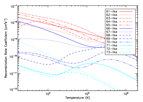
Figure 1: Total DR rate coefficients calculated in level resolution (except for 63- and 71-like, calculated in configuration resolution) for 61- to 73-like.

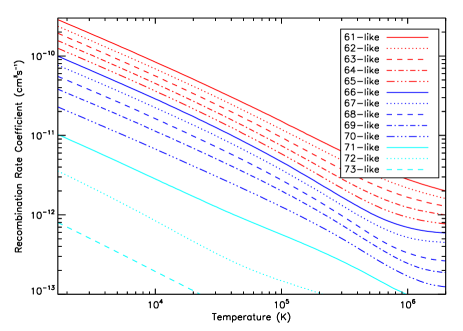
Figure 2: Total RR rate coefficients calculated in level resolution (except for 63- and 71-like, calculated in configuration resolution) for 61- to 73-like.

In this section we discuss the results of the calculations. In Figures 1 and 2 we have plotted the total DR rate coefficients for 61- to 73-like in level resolution (except for 63- and 71-like, plotted in configuration resolution), and the total RR rate coefficients calculated in level resolution respectively. We consider each ionization state in turn, and compare the contribution of each core excitation to the total recombination rate coefficient. When comparing the core excitations, we also indicate the peak fraction for that particular ion, calculated using the recombination rate coefficients of Pütterich et al [3], and the ionization rate coefficients of Loch et al [48]. For each ionization state, we also indicate what value of $\lambda_{n\ell}$ was used to produce the correct ground state as listed on the NIST website [49, 50, 51]. Note that odd parity states are indicated with an $*$ superscript in front of the level symbol.

4.1 61-like: W¹³⁺

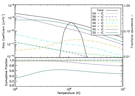
Figure 3: Contributions to the total recombination rate coefficient for 61-like (top plot), and their cumulative fractions (bottom plot), calculated in IC. The method for calculating the cumulative fractions is given in text.

The ground state listed by NIST for this ion is $4f^{13}5s^{2}$ ${}^{2}F^{*}_{7/2}$. We set $\lambda_{n\ell}=0.99$ to reproduce this ground state in autostructure. In Figure 3 we have plotted the individual contributions to the total recombination rate coefficients for 61-like, calculated in IC. The top plot shows the individual recombination rate coefficients as compared to the total, along with the peak abundance fraction (solid parabola) for 61-like. The bottom plot shows the cumulative contribution for each core excitation. This is calculated by summing the individual contributions, from largest to smallest, up to the core excitation being considered. This sum is then divided by the total recombination rate coefficient. The largest contribution to the recombination rate total comes from the 5–5 core excitation, contributing 62% at peak abundance temperature ($1.16\times{10}^{6}$K). This is followed by the 4–5 core excitation, which contributes 30%. The remaining 10% is comprised of 4–4, 4–6, RR, 5–6, and 5–4. The 5–5 core excitation is strongest around the peak abundance. 5–5 decreases to 10% of the recombination rate total towards the lowest temperature considered (1690K). Towards higher temperatures, 5–5 decreases steadily, constituting 35% of the total by $\sim{3}\times{10}^{8}$K. The 4–5 core excitation is strongest at low temperatures, consituting 84% of the recombination rate total at the lowest temperature considered. Towards higher temperatures, 4–5 decreases to 23% of the total. RR only becomes significant towards higher temperatures, constituting 25% of the recombination rate total at $\sim{3}\times{10}^{8}$K.

4.2 62-like: W¹²⁺

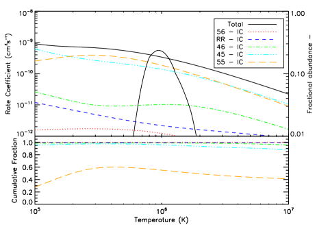
Figure 4: Contributions to the total recombination rate coefficient for 62-like (top plot), and their cumulative fractions (bottom plot), calculated in IC.

The ground state given by NIST for this ion is $4f^{14}5s^{2}$ ${}^{1}S_{0}$. To reproduce the correct ground state in autostructure we set $\lambda_{nl}=0.98$. This ion was calculated in both IC and CA. In Figure 4 we have plotted the individual core excitations and their contributions to the recombination rate totals, along with their cumulative fractions. The largest contributions to the total comes from the 4–5 and 5–5 core excitations, contributing 41 and 55% to the recombination rate total at peak abundance temperature ($9.4\times{10}^{5}$K) respectively. This is followed by the 4–6 core excitation, which only contributes 3% to the total. The remainder of the total is composed of the 5–6 core excitation, and RR. Towards lower temperatures, the contribution of the 5–5 core excitation peaks at $\sim{4}\times{10}^{5}$K, consituting 60% of the recombination rate total. The contribution from 5–5 then steadily decreases to 11% at $\sim{20000}$K, followed by a slight increase to 23% at $\sim{1000}$K. The contribution from 5–5 decreases steadily with increasing temperature, constituting $\sim{30}$% of the total by $\sim{1}\times{10}^{8}$K. The contribution from the 4–5 core excitation peaks at $\sim{17000}$K, consituting 84% of the recombination rate total. Towards lower temperatures, the contribution from 4–5 decreases steadily from its peak value, constituting 73% of the total by $\sim{1000}$K. Towards higher temperatures, the contribution from 4–5 again decreases steadily from it’s peak value, constituting $\sim{40}$% of the total by $\sim{1}\times{10}^{8}$K. The contribution from RR is very small below peak abundance temperatures, constituting only 3% of the total at $\sim{1000}$K. However, there is a larger contribution from RR at the highest temperatures considered, constituting $\sim{20}$% of the total at $\sim{1}\times{10}^{8}$K.

4.3 63-like: W¹¹⁺

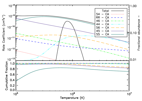
Figure 5: Contributions to the total recombination rate coefficient for 63-like (top plot), and their cumulative fractions (bottom plot), calculated in CA.

This ionization state was calculated in CA only, as a representative calculation done in IC is too computationally expensive at present. By setting $\lambda_{nl}=1.00$, autostructure predicts the ground state configuration to be $4f^{13}5s^{2}5p^{2}$ ${}^{4}F^{*}_{7/2}$. As this is in agreement with the value given by NIST, we do not alter $\lambda_{nl}$. The individual contributions to the total recombination rate coefficient for this ionization state are plotted in Figure 5, along with their cumulative fractions. The largest contributions to the total comes from the 4–5 and 5–5 core-excitations, contributing $\sim{11}$ and $\sim{84}$% to the total at peak abundance temperature ($8.1\times{10}^{5}$K) Towards lower temperatures, the 5–5 core excitation gives way to 4-5, with the latter constituting $\sim{92}$% of the recombination rate total. 4–4 is the next largest contribution after 4–5 and 5–5, constituting $\sim{13}$% of the total at $\sim{3}\times{10}^{7}$K. The 4–6 core-excitation contributes very little for all temperatures, consituting a maximum of $\sim{3}$% of the total at $\sim{7}\times{10}^{4}$K. The 5–4 core-excitation contributes $<1$% for all temperatures, and 5–6 only constitutes $\sim{3}$% at maximum for temperatures $>1\times{10}^{6}$K. RR contributes little to the recombination rate total over all but the highest temperatures. At peak abundance temperature, RR contributes $<1$%, whereas at the highest temperature considered ($2.4\times{10}^{8}$K), RR contributes $\sim{17}$%. At low temperatures of $\sim{1000}$K, RR constitutes $\sim{7}$% of the total.

4.4 64-like: W¹⁰⁺

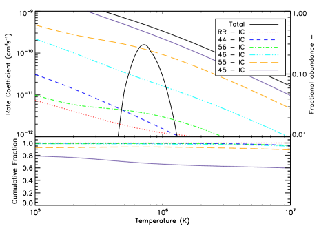
Figure 6: Contributions to the total recombination rate coefficient for 64-like (top plot), and their cumulative fractions (bottom plot), calculated in IC.

The DR/RR rate coefficients for this ion were calculated in IC and CA. To reproduce the ground state as given on the NIST website ($4f^{14}5s^{2}5p^{2}$ ${}^{3}P^{*}$), we set $\lambda_{n\ell}=0.99$. We plot the individual contributions to the recombination rate total for 64-like in Figure 6, along with their cumulative fractions. At peak abundance temperature ($7.14\times{10}^{5}$K) the total is dominated by the contributions of the 4–5 and 5–5 core excitations, constituting 68 and 26% to the total respectively. This is followed by the 4–6 core excitation, contributing 5% to the total. 4–4, 5–6, and RR contribute very little to the total at peak abundance temperature. Combined, 4–4, 5–6, and RR constitute $<1$% of the recombination rate total. The contribution of the 4–5 core excitation decreases steadily with increasing temperature, constituting $\sim{50}$% of the total by $\sim{1}\times{10}^{8}$K. The converse is true for decreasing temperature, with the contribution from 4–5 constituting 90% at the lowest ADAS temperature considered for this ion (1000K). The contribution from 5–5 peaks at $\sim{4}\times{10}^{6}$K, constituting $\sim{30}$% of the total. For higher temperatures than this peak, the contribution from 5–5 decreases steadily, constituting 24% of the total by $\sim{1}\times{10}^{8}$K. For lower temperatures than the peak, the contribution from 5–5 again decreases steadily, constituting just $\sim{2}$% at 1000K. The contribution from 4–6 over the entire temperature range is small, but non-negligible, constituting 4–7% over the entire ADAS temperature range. The contribution from 4–4 and 5–6 is negligible at all temperatures. RR only becomes significant at the highest temperatures, constituting 20% of the total at $\sim{1}\times{10}^{8}$K.

4.5 65-like: W⁹⁺

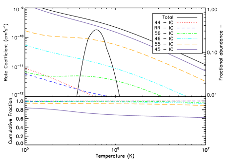
Figure 7: Contributions to the total recombination rate coefficient for 65-like (top plot), and their cumulative fractions (bottom plot), calculated in IC.

For this ionization state, NIST lists the ground state configuration as being $4f^{14}5s^{2}5p^{3}$ ${}^{2}P^{*}_{3/2}$. To reproduce this ground state, we set $\lambda_{n\ell}=0.99$. In Figure 7 we have plotted the individual contributions to the recombination rate total for 65-like, along with their cumulative fractions. The recombination rate total is dominated by the 4–5 and 5–5 core excitations at peak abundance temperature ($6.18\times{10}^{5}$K), constituting 70 and 23% of the total respectively. The contribution from 4–6 is smaller than in the case of 64-like, constituting $\sim{4}$% of the total. The 4–5 contribution decreases steadily with increasing temperature, constituting 50% of the total at $\sim{1}\times{10}^{8}$K. As with 64-like, the 4–5 contribution increases with decreasing temperature, constituting 96% of the total for the lowest ADAS temperature considered for this ion (810K). The contribution from 5–5 peaks at $\sim{5}\times{10}^{6}$K, constituting 28% of the total. For increasing temperatures above this peak, 5–5 decreases steadily, constituting 22% at $\sim{1}\times{10}^{8}$K. Below this peak temperature, 5–5 decreases steadily with decreasing temperature, constituting just 3% at the lowest ADAS temperature considered. The 4–6 contribution to the total peaks at $\sim{5}\times{10}^{6}$K, constituting 4% of the total. With increasing temperature from this peak, the contribution from 4–6 decreases to 3% by $\sim{1}\times{10}^{8}$K. The contribution from 4–6 becomes negligible with decreasing temperature below the peak. At maximum, the 5–6 core excitation contributes 2% to the total. The 4–4 core excitation is completely negligible, and contributes $<1$% to the total for the entire ADAS temperature range. RR again is only significant at high temperatures, constituting 22% of the total at $\sim{1}\times{10}^{8}$K.

4.6 66-like: W⁸⁺

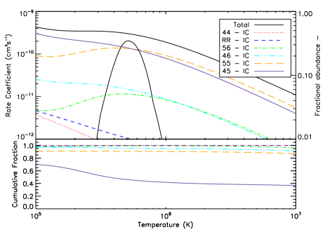
Figure 8: Contributions to the total recombination rate coefficient for 66-like (top plot), and their cumulative fractions (bottom plot), calculated in IC.

The ground state for this ion is $4f^{14}5s^{2}5p^{4}$ ${}^{3}P_{2}$ In order to reproduce this in autostructure, we set $\lambda_{n\ell}=0.99$. In Figure 8 we plot the individual contributions to the recombination rate total, and their cumulative fractions. At peak abundance temperature ($5.14\times{10}^{5}$K) the largest contributions to the total come from the 4–5 and 5–5 core excitations, constituting 46 and 45% of the total respectively. These are followed by the 4–6 and 5–6 core excitations, contributing 5 and 4% to the total respectively. The 4–5 contribution decreases with increasing temperature, constituting 30% of the total at $\sim{1}\times{10}^{8}$K. With decreasing temperature, the contribution of 4–5 increases steadily, peaking at $\sim{5000}$K, and constituting 71% of the total. The contribution from 4–5 then decreases slightly to 69% of the total at the lowest ADAS temperature considered (640K). The 5–5 contribution peaks at $\sim{4}\times{10}^{6}$K, constituting $\sim{50}$% of the total. The contribution from 5–5 then decreases steadily with increasing temperature above the peak, constituting $\sim{42}$% of the total. With decreasing temperature below the peak, the contribution from 5–5 again decreases, constituting 25% of the total at $\sim{1000}$K. The contribution from 4–6 peaks at $\sim{2}\times{10}^{5}$K, constituting 6% of the total. The contribution from 4–6 decreases with increasing temperature above the peak, constituting 4% at $\sim{1}\times{10}^{8}$K. With decreasing temperature below the peak, the contribution from 4–6 decreases steadily to 5% at $\sim{1000}$K. The 4–4 core excitation, as in the case of 65-like, is negligible, contributing $<1$% for the entire ADAS temperature range. RR, again, is only significant at high temperatures, constituting 20% of the total at $\sim{1}\times{10}^{8}$K.

4.7 67-like: W⁷⁺

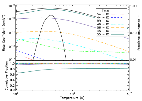
Figure 9: Contributions to the total recombination rate coefficient for 67-like (top plot), and their cumulative fractions (bottom plot), calculated in IC.

For this ion, we set $\lambda_{nl}=0.98$ to reproduce the correct ground state as listed on the NIST website ($4f^{13}5s^{2}5p^{6}$ ${}^{2}F^{*}_{7/2}$). We have plotted the individual contributions to the total recombination rate coefficients for 67-like, as well as their respective cumulative fractions, in Figure 9. The 5–5 core excitation is the largest contributor, constituting 78% of the total at peak abundance temperature ($4.2\times{10}^{5}$K). This is followed by 4–5, contributing 19% to the total, and 5–6, contributing 2%. The contributions from 5–5 and 4–5 do not vary much with respect to temperature, with the contribution from 5–5 ranging from $\sim{60}$–80% of the total, and the contribution from 4–5 ranging from 15-30% of the total. The 5–6 contribution is small over the entire ADAS temperature range. At maximum, 5–6 contributes 3% to the total at $\sim{10,000}$K. The 4–4, 5–4, and 4–6 core excitations are completely negligible. Combined, these core excitations constitute $<1$% of the recombination rate total for the entire ADAS temperature range. RR again is significant at higher temperatures albeit much less so than in the case of preceeding ions, constituting just 6% of the total at $\sim{5}\times{10}^{7}$K.

4.8 68-like: W⁶⁺

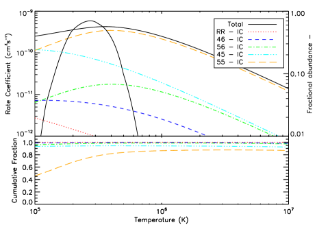
Figure 10: Contributions to the total recombination rate coefficient for 68-like (top plot), and their cumulative fractions (bottom plot), calculated in IC.

We set $\lambda_{nl}=0.98$ for this ion to reproduce the correct ground state as listed on the NIST website ($4f^{14}5s^{2}5p^{6}$ ${}^{1}S_{0}$). In Figure 10 we have plotted the individual contributions to the recombination rate total for 68-like, and their respective cumulative fractions. At peak abundance temperature ($2.74\times{10}^{5}$K) the majority of the total recombination rate coefficient is composed of the 5–5 and 4–5 core excitations, constituting 76 and 19% of the total respectively. This is followed by 5–6 and 4–6, constituting 4 and 2% of the total respectively. The 5–5 core excitation contribution to the total has two maxima. The first is at $\sim{1}\times{10}^{4}$K, constituting 62% of the total, and the second is at $\sim{3}\times{10}^{6}$K, constituting 88% of the total. Towards the lowest temperatures considered, the contribution from 5–5 deminishes, contributing $\sim{50}$% to the total by $\sim{1000}$K. With increasing temperature, the contribution from 5–5 remains large, constituting 82% of the total at $\sim{5}\times{10}^{7}$K. The 4–5 contribution peaks at $\sim{5}\times{10}^{6}$K, contributing 56% to the total. With increasing temperature above this peak, the contribution from 4–5 decreases quite rapidly, constituting only 5% of the total by $\sim{5}\times{10}^{7}$K. With decreasing temperature below the peak, the contribution from 4–5 again decreases rapidly, contributing 6% at $\sim{1000}$K. The 5–6 core excitation does not contribute much over the ADAS temperature range, providing a peak contribution of 5% at $\sim{5}\times{10}^{6}$K. The contribution from 4–6 is the smallest for the entire ADAS temperature range, contributing a maximum of $\sim{3}$% to the total at $\sim{4}\times{10}^{4}$K. As with the preceeding ions, the contribution from RR is negligible at peak abundance temperature. However, RR becomes far more significant towards lower temperatures, contributing 45% to the total recombination rate coefficient at $\sim{1000}$K.

4.9 69-like: W⁵⁺

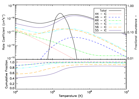
Figure 11: Contributions to the total recombination rate coefficient for 69-like (top plot), and their cumulative fractions (bottom plot), calculated in IC.

For this ion, we set $\lambda_{nl}=0.97$ to reproduce the correct ground state as listed on the NIST website ($5p^{6}5d$ ${}^{2}D_{3/2}$). In Figure 11 we have plotted the individual contributions to the total recombination rate coefficient for 69-like calculated in IC, as well as their respective cumulative fractions. The 5–5 core excitation is dominant at peak abundance temperature ($1.63\times{10}^{5}$K), contributing 69% to the recombination rate total. The next largest contribution comes from the 5–6 core excitation, contributing 15% to the total. This is followed by 4–5, constituting 13% of the total. The remainder of the total is comprised of RR, 4–6, and 4–4, contributing a combined $\sim{3}$%. The contribution from 5–5 peaks at $\sim{3}\times{10}^{6}$K, contributing 85% to the total. For increasing temperature above this peak, the contribution decreases slightly, constituting 77% of the total at $\sim{5}\times{10}^{7}$K. For decreasing temperature below the peak, the contribution from 5–5 decreases gradually, constituting 25% of the total by $\sim{1000}$K. For temperatures $\leq{1}\times{10}^{5}$K the contribution from the 5–6 core excitation is relatively steady, constituting 10-20% of the total. Above this temperature, the contribution from 5–6 decreases slowly, constituting 5% of the total at $\sim{5}\times{10}^{7}$K. The contribution from the 4–5 core excitation peaks at $\sim{3000}$K, contributing 24% to the total. For increasing temperature above this peak, the contribution from 4–5 decreases slowly, constituting 6% at $\sim{5}\times{10}^{7}$K. For decreasing temperature below the peak, the contribution from 4–5 decreases rapidly, contributing $<1$% at the lowest ADAS temperature considered (250K). The 4–6 core excitation contributes very little over the entire ADAS temperature range.At maximum, 4–6 contributes 2% to the total, but only for temperatures $\geq{1}\times{10}^{5}$K The 4–4 core excitation is only significant for low temperatures. At $\sim{1000}$K 4–4 contributes 21% to the total. The contribution from RR is more significant towards lower temperatures, contributing 24% to the total at $\sim{1000}$K. However, at higher temperatures, RR is non-negligible, contributing 11% to the total at $\sim{5}\times{10}^{7}$K.

4.10 70-like: W⁴⁺

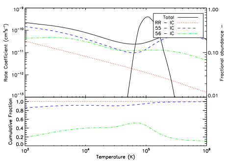
Figure 12: Contributions to the total recombination rate coefficient for 70-like (top plot), and their cumulative fractions (bottom plot), calculated in IC.

To date, no detailed calculations of DR rate coefficients have been performed for this ion up to 73-like. Thus, the present work constitutes the first such calculations. In Figure 12 we have plotted the recombination rate coefficients for 5-5, 5-6, and RR for 70-like, calculated in IC. Setting $\lambda_{nl}=0.96$ gives the correct ground state of $5p^{6}5d^{2}$ ${}^{3}F_{2}$ as listed on NIST. The contributions from 5-5 and 5-6 are comparable at peak abundance temperature ($7.0\times{10}^{4}$K), constituting 41 and 51% of the recombination rate coefficient total respectively. Interestingly, the peak abundance temperature marks the largest contribution to the recombination rate total for 5-6. For temperatures greater than the peak abundance temperature, the contribution from 5-6 decreases steadily. By $\sim{3}\times{10}^{7}$K, 5-6 contributes only 8% to the recombination rate total. Likewise, for temperatures less than the peak abundance temperature, the contribution from 5-6 steadily decreases to 2% at $\sim{200}$K. The largest contribution from 5-5 occurs at $\sim{10}^{6}$K, constituting $\sim{90}$% of the recombination rate total. For temperatures $\geq{10}^{6}$K the contribution from 5-5 decreases steadily from its maximum to $\sim{76}$% at $\sim{3}\times{10}^{7}$K. For temperatures $\leq{10}^{6}$K the 5-5 contribution decreases to 41% at the peak abundance temperature, after which the contribution begins increasing again, constituting 63% of the total at $\sim{200}$K. RR contributes little at peak abundance temperature, constituting 7% of the recombination rate total. For temperatures greater than the peak abundance temperature, the contribution from RR decreases slightly, and then gradually increases with increasing temperature, constituting 16% of the recombination rate total at $\sim{3}\times{10}^{7}$K. For temperatures less than the peak abundance temperature, the contribution from RR increases gradually, constituting 34% of the total at the lowest temperature considered for this ion ($\sim{200}$K).

4.11 71-like: W³⁺

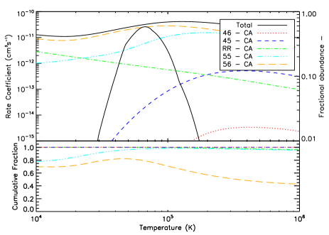
Figure 13: Contributions to the total recombination rate coefficient for 71-like (top plot), and their cumulative fractions (bottom plot), calculated in CA.

The recombination rate coefficients for this ionization state were calculated in CA only, and are plotted in FIgure 13. We set $\lambda_{nl}=0.96$ to reproduce the correct ground state as listed on NIST ($5p^{6}5d^{3}$ ${}^{4}F_{3/2}$). The largest contributions to the recombination rate total come from the 5-5 and 5-6 core excitations, contributing $\sim{28}$ and 70% to the total at peak temperature respectively. The 4-5 and 4-6 core excitations contribute very little to the total over the entire ADAS temperature range. The 4-5 core excitation contributes $\sim{3-4}$% to the total for temperatures $>7\times{10}^{5}$K, while the 4-6 core excitation contributes $<1$% for all temperatures. At temperatures $>1.8\times{10}^{7}$K, 5-5, 5-6, and RR contribute to the total equally, composing $\sim{33}$% of the recombination rate total. Towards the lowest temperature considered for this ion (90K), the recombination rate total is dominated by RR, constituting 100% of the total.

4.12 72-like: W²⁺

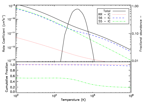
Figure 14: Contributions to the total recombination rate coefficient for 72-like (top plot), and their cumulative fractions (bottom plot), calculated in IC.

In Figure 14 we have plotted the individual contributions to the total recombination rate coefficients for 72-like, along with their cumulative fractions. To reproduce the ground state listed on NIST ($5p^{6}5d^{4}$ ${}^{5}D_{0}$), we set $\lambda_{nl}=0.96$. This value also improves the general agreement between the autostructure energies, and the values listed on NIST. At peak abundance temperature ($2.9\times{10}^{4}$K), the contributions from 5–5 and 5–6 are nearly equal, constituting 47 and 52% of the recombination rate total respectively. The 5–5 core excitation provides the largest contribution at $\sim{200}$K, constituting 61% of the recombination rate total. For temperatures $<200$K, 5–5 decreases slightly, constituting 48% of the recombination rate total at $\sim{40}$K. Caution should be taken in interpreting this result, as low temperature DR is very sensitive to the positioning of resonances at threshold. The 5–5 contribution steadily decreases for increasing temperature, and constitutes only $\sim{10}$% of the recombination rate total at $\sim{8}\times{10}^{6}$K. For 5–6, the largest contribution occurs at $\sim{5}\times{10}^{5}$K, constituting 77% of the recombination rate total. This decreases to 38% at $\sim{200}$K, and then increases slightly to 51% at $\sim{40}$K. It is interesting to note that the contribution from 5–6 is larger than that of 5–5 at low temperatures. As the $6s$ orbital encroaches upon the $5d$ orbital, it is energetically more favourable for transitions to $6s$ to occur at low temperatures. The contribution from RR is small for temperatures $<1.8\times{10}^{6}$K, constituting $<10$% of the recombination rate total. For higher temperatures, the contribution from RR increases gradually to 47%, becoming comparable to the 5–6 contribution.

4.13 73-like: W¹⁺

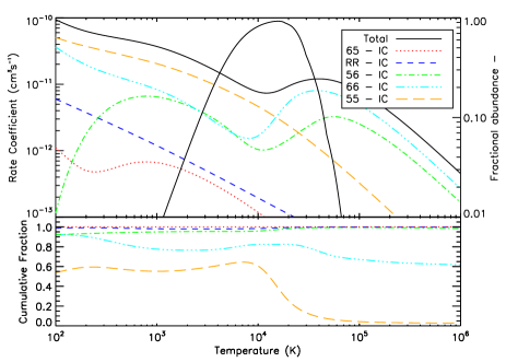
Figure 15: Contributions to the total recombination rate coefficient for 73-like (top plot), and their cumulative fractions (bottom plot), calculated in IC.

We have plotted the individual contributions to the recombination rate total for 73-like in Figure 15, calculated in IC. We set $\lambda_{nl}=0.96$, to reproduce the correct ground state as listed by NIST ($5d^{4}6s$ ${}^{6}D_{1/2}$). This also improves the general agreement between the autostructure energies, and those listed on the NIST website. At peak abundance temperature ($1.6\times{10}^{4}$K) there is an interesting competition between the 5–5, 5–6, and 6–6 core excitations. The 5–5 core excitation experiences a sharp drop in its contribution to the recombination total, constituting $\sim{60}$% of the total at $\sim{10,000}$K, followed by a rapid drop to just $\sim{10}$% at 37,000K. This is a result of the 5–6 and 6–6 DR rate coefficients peaking at 40,000 and 60,000K respectively, corresponding to the $5d\rightarrow{6s}$ and $6s\rightarrow{6p}$ promotions respectively. The sharp drop in the contribution is compensated for by 6–6, contributing $\sim{20}$% at $\sim{10,000}$K, followed by a sharp rise to $\sim{65}$% by $\sim{37,000}$K. The contribution from 5–6 is fairly constant, constituting 15% of the total at peak abundance temperature. The contribution from 5–5 decreases steadily with increasing temperature, constituting just 3% at $\sim{1}\times{10}^{6}$K. Below peak abundance temperature, the contribution remains constant with decreasing temperature, constituting $\sim{50}$% of the total. The 6–5 core excitation is negligible, and contributes $<2$% over the entire ADAS temperature range. The contribution from RR is small for all temperatures. At maximum, RR contributes 6% to the total at $\sim{100}$K.

5 Comparison with other works

As discussed in the introduction, the lanthanide series and beyond are relatively unexplored areas in terms of DR rate coefficient calculations. The only available detailed calculations are from Safronova et al covering W⁵⁺-W⁶⁺ [16, 17], and Kwon covering W⁵⁺-W¹⁰⁺ [34]. The DR rate coefficients from Kwon were calculated using FAC [28], while the DR rate coefficients from Safronova et al were calculated using a combination of hullac [15], and the Cowan atomic structure code. In the absence of experimental data (such as those from storage ring experiments), comparisons between DR rate coefficients calculated using different codes offer an alternative method with which to benchmark these data. In general, the DR rate coefficients for a particular ion at low temperatures can be highly uncertain due to the positioning of resonances. This is especially so in the case of low-ionization state tungsten, as calculating an accurate structure for such ions can be prohibitively difficult.

5.1 64-like: W¹⁰⁺

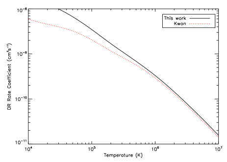
Figure 16: Comparison between the total DR rate coefficients for 64-like W, calculated in this work (solid black), and Kwon [34] (red-dotted).

In Figure 16 we have plotted the total DR rate coefficient for 64-like as calculated in the present work, and by Kwon [34]. At peak abundance temperature ($\sim{7}\times{10}^{5}$K) we find our rates differ from Kwon’s by 14%. This difference decreases with increasing temperature, with our results differing by 10% at $2\times{10}^{8}$K. For lower temperatures, our results and Kwon’s diverge significantly, with the largest difference occuring at $1\times{10}^{4}$K of 68%.

5.2 65-like: W⁹⁺

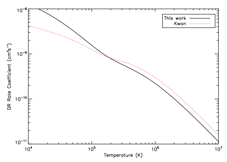
Figure 17: Comparison between the total DR rate coefficients for 65-like W calculated in this work (solid black), and Kwon [34] (red-dotted).

We have plotted the total DR rate coefficients for 65-like as calculated in the present work in Figure 17, along with the result calculated by Kwon [34]. Reasonable agreement is seen at peak abundance temperature ($6.2\times{10}^{5}$K), with Kwon’s result being $32\%$ larger than the present work. This difference increases slightly with increasing temperature, reaching 38% at $1.6\times{10}^{8}$K. Agreement also deteriorates towards lower temperatures, with Kwon’s DR rate coefficient being $\sim{70}$% smaller than the present work for temperatures $<1000$K.

5.3 66-like: W⁸⁺

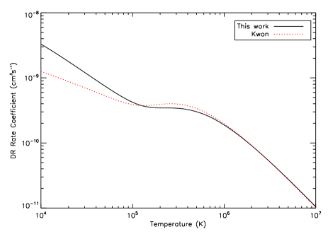
Figure 18: Comparison between the total DR rate coefficients for 66-like W calculated in this work (solid black), and Kwon [34] (red-dotted).

In Figure 18 we have plotted the total DR rate coeffcients as calculated in the present work, and by Kwon [34]. Good agreement is seen at peak abundance temperature ($5.1\times{10}^{5}$K), with Kwon’s DR rate coefficients being larger than the present work by 11%. Agreement improves to better than 10% for temperatures $>6\times{10}^{5}$K. The largest differences are seen at lower temperatures, being $>80$% for temperatures $<$ 1000K.

5.4 67-like: W⁷⁺

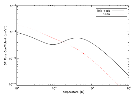
Figure 19: Comparison between the total DR rate coefficients for 67-like W calculated in this work (solid black), and Kwon [34] (red-dotted).

In Figure 19 we have plotted the total DR rate coefficients for 67-like as calculated in the present work, and by Kwon [34]. Significant differences are seen between both sets of DR rate coefficients across a wide range of temperatures. At peak abundance temperature ($4.2\times{10}^{5}$K), Kwon’s DR rate coefficients are $\sim{60}$% smaller than ours. With increasing temperature, the difference between our and Kwon’s DR rate coefficients becomes constant, reaching $\sim{83}$% at $\sim{1}\times{10}^{8}$K. Towards lower temperatures, the largest difference between our data and Kwon’s is seen at $\sim{1000}$K, where Kwon’s DR rate coefficients are larger by a factor $\sim{3}$.

5.5 68-like: W⁶⁺

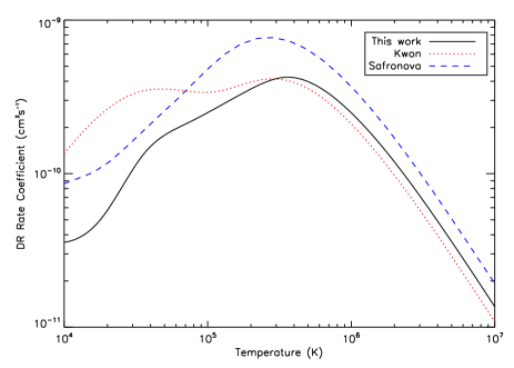
Figure 20: Comparison between the total DR rate coefficients for 68-like W calculated in this work (solid black), Kwon [34] (red-dotted), and Safronova et al [17] (blue-dash).

DR rate coefficients for this ion have been calculated by Kwon [34] and Safronova et al [16, 17]. In Figure 20 we have plotted their results, along with those calculated in this current work. Poor agreement is evident over a wide range of temperatures. However, at peak abundance temperature ($2.7\times{10}^{5}$K), Kwon’s DR rate coefficients are larger by $\sim{2}$%, while Safronova et al ’s are larger by a factor $\sim{2}$. Given the variation of the DR rate coefficient either side of the peak abundance temperature, this agreement appears to be coincidental. Towards higher temperatures ($>3\times{10}^{6}$K) the difference between our data and Kwon’s remains constant, with Kwon’s DR rate coefficients being $\sim{20}$% smaller than the present calculation. In the case of Safronova’s data for these temperatures, the difference varies from $\sim{40}-90$% larger than the present values. Towards lower temperatures, the difference between all datasets diverge strongly, with the largest differences exceeding $\sim{9}$ dex at the lowest temperatures.

5.6 69-like: W⁵⁺

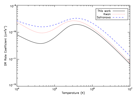
Figure 21: Comparison between the total DR rate coefficients for 69-like W calculated in this work (solid black), Kwon [34] (red-dotted), and Safronova et al [16] (blue-dash).

As with 68-like, DR rate coefficients have been calculated by Kwon [34] and Safronova et al [16, 17]. In Figure 21 we have plotted our results, along with those of Kwon and Safronova et al . The general trend of all three calculations appear to be in agreement. At peak abundance temperature ($1.7\times{10}^{5}$K) the DR rate coefficients calculated by Kwon and Safronova are larger than the present data by $\sim{80}$% and a factor $\sim{2}$ respectively. Towards higher temperatures the agreement between the present data and Kwon’s results improves, with Kwon’s DR rate coefficients being larger by $\sim{13}$%. This is not the case for Safronova et al ’s data, where the difference varies between a factor 1.7-2.0 with increasing temperature. Agreement does not improve with decreasing temperature, with differences of a factor $\sim{9}$ and $\sim{4}$ for Kwon and Safronova et al respectively.

6 Ionization State Evolution

In this section we consider the impact of our calculations in the context of ionization fractions. We first consider the steady state ionisation fraction incorporating our data, and lastly, we consider a time-dependent case.

6.1 Steady state ionization

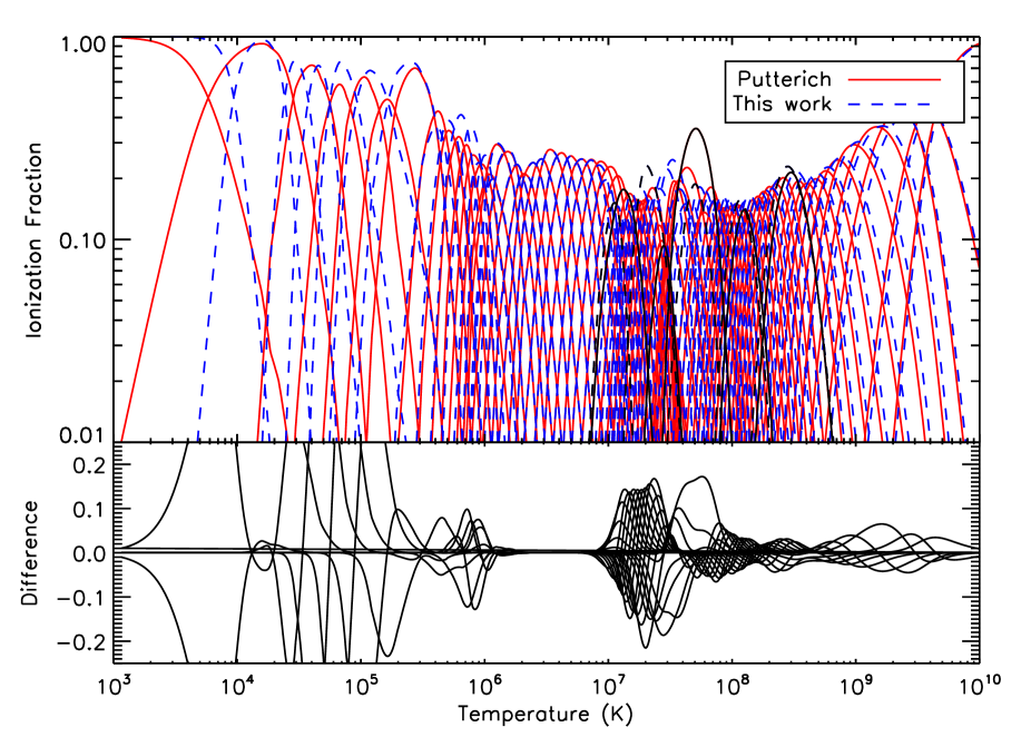
Figure 22: Plot of the coronal, steady-state ionization fraction for tungsten. The red fraction was calculated using the recombination rate coefficients of Pütterich et al [3], and the ionization rate coefficients of Loch et al [48]. The blue-dashed fraction was calculated using the recombination rate coefficients calculated in this work (61- to 73-like), and the data from previous work by Preval et al [11, 12, 13] (00- to 46-like). We used Pütterich et al ’s data for 47- to 60-like. From right to left, we have indicated the positions of the closed-shell states 10-, 18-, 28-, 36-, and 46-like with black parabolas. The bottom plot is the arithmetic difference between the Pütterich et al fractions, and the present fraction.

We now compare two sets of ionization fractions, calculated using recombination rate coefficient data from this work (61- to 73-like) and The Tungsten Project (00- to 46-like, [11, 12, 13]), and using the scaled data from Pütterich et al [3]. For the ionization fraction calculated using the present data, we use the data from Pütterich et al for 47- to 60-like, as we have not calculated data for these charge states yet. In both cases, we use the ionization rate coefficients as calculated by Loch et al [48]. The two ionization fractions are plotted in Figure 22, along with the arithmetical difference between the two fractions. We have also indicated the position of closed-shell charge states as a guide. In this plot, there is a large gap indicating zero difference between the two fractions. This is because the data for 47- to 60-like are the same in both fractions. Immediately obvious is the significant differences in the peak abundance temperature, and the peak abundance fractions. In Table LABEL:table:peaktemp we have listed these peak fractions and temperatures for our ionization fraction, and that of Pütterich et al . We have also calculated the % difference between the peak temperatures and fractions calculated in this work, and those from Pütterich et al .

Looking at the plot overall, it is clear that the largest differences between our ionization fraction and Pütterich et al ’s occurs for 61- to 73-like. This is indicative of the difference in atomic structures used in both approaches, and also highlights the difficulty in calculating a reliable atomic structure. As mentioned in Section 5, relatively good agreement between our calculations and Kwon’s [34] is seen for the higher ionization states. For the lower ionization states, this agreement deteriorates. Further calculations by other groups using different codes could help to improve our understanding of the atomic structure for these ions.

6.2 Time-dependent ionization

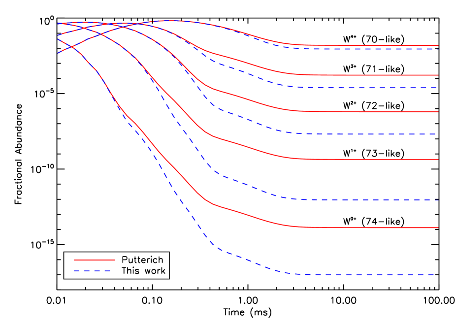
Figure 23: Time evolution of the charge state distribution of 74- to 70-like tungsten for a 20eV plasma over 100ms. The red solid line is the case where the recombination rate coefficients of Pütterich et al [3] were used, whereas the blue dashed line is the case where the present recombination rate coefficients were used.

To further illustrate the impact of our data, we considered the time evolution of the ionization fractions for a 20eV, fixed density plasma where a tungsten impurity was introduced. This was done using the ADAS406 routine, the description for which can be found on the ADAS website. In Figure 23 we have plotted the evolution of five charge states spanning 70- to 74-like over a period of 100ms using the present data, and the recombination rate coefficients of Pütterich et al . While ionization is the dominant process, it can be clearly seen that the recombination rate coefficients determine the final equilibrium state. The differences seen can easily be attributed to the methods used in calculating the recombination rate coefficients.

7 Conclusions

We have presented a series of partial, final-state resolved DR and RR rate coefficients for low-charge tungsten ions spanning W¹³⁺ - W¹⁺. The present work constitutes the first such DR/RR calculations performed for low ionization state tungsten. These data will be paramount in modelling the collisional-radiative properties of the edge plasma in magnetically confined, finite density plasmas such as those observed in JET and ITER.

We calculated an updated coronal, steady-state ionization balance for tungsten using all of the recombination rate coefficient data calculated in The Tungsten Project, and the ionization rate coefficients from Loch et al [48]. We compared this with an ionization balance calculated using the recombination rate coefficients of Pütterich et al [3], and found significant differences between the two fractions. In particular, there were large shifts in the peak fractions and temperatures. The majority of these large changes were for the lowest ionization states considered, illustrating the difficulty in calculating an accurate atomic structure for these ions.

We find our DR rate coefficients are in relatively good agreement with the few currently published, and we are able to reproduce the general trend of these data. This is in contrast to the case of more highly-charged ions where substantial differences were found. However, large differences are seen towards lower temperatures. While this isn’t a problem in the case of highly charged states, in the case of singly, doubly, or triply ionized ions the peak abundance temperature and peak fraction will be sensitive to threshold effects. This was also evidenced by considering a time-dependent ionization fraction using the ADAS routine ADAS406. It was shown that for a fixed density, 20 eV plasma with a tungsten impurity, the recombination rate coefficients used for 70- to 73-like had a significant impact on the final equilibrium state. Therefore, more work is required to constrain the DR rate coefficients further for these ionization states.

The main challenge in improving the DR rate coefficients for low ionization state tungsten lies in constraining the positioning of near-threshold resonances. As well as extensive theoretical work, experiment must also be used. Cryogenic storage ring experiments such as those described in Spruck et al [52] and Von-Hahn et al [53] can potentially be used in the case of low charge-state tungsten ions. As seen in Figure 23, significant differences were seen in the final equilibrium state of a 20 eV plasma with a tungsten impurity when using the present data, or that of Pütterich et al [3]. The largest differences between the two cases was seen for neutral-state tungsten. However, this difference decreased with increasing residual charge, indicating a larger uncertainty in the DR rate coefficients for the lowest charge states. Therefore, future experiments should focus on the near-neutral charge states of tungsten.

The data presented in this paper, combined with our work on the $4d$-shell tungsten ions, gives an indication of how the missing $4f$-shell DR rate coefficients will behave when they are added. Currently, the open $4f$-shell problem in calculating DR rate coefficients is still untenable by even the best computational systems without implementing some form of statistical approximation. It is possible in the near future that a fully parallelised version of autostructure could tackle this problem. The final paper in The Tungsten Project will consider the $4f$ shell as far as is possible with autostructure. We will then use a partitioning method as described in Badnell et al [38] to cover any ions we cannot compute directly.

References

Table 1: List of core $N$-electron configurations included in our calculations for each charge state. The $(N+1)$-electron configurations were obtained by adding an additional electron to all of the $N$-electron configurations. We also indicate the core excitations extracted from these calculations.

Ion-like	Core excitations	N-electron configurations
61-like	4–4, 4–5, 4–6, 5–4,	$4d^{10}4f^{13}5snl$, $n=4-6$, $\ell=0-5$
	5–5, 5–6	$4d^{10}4f^{12}5s^{2}nl$, $n=5-6$, $\ell=0-5$
		$4d^{9}4f^{13}5s^{2}nl$, $n=4-6$, $\ell=0-5$
		$4d^{10}4f^{13}6s^{2}$
		$4d^{10}4f^{13}6s6p$
		$4d^{10}4f^{13}6p^{2}$
62-like	4–5, 4–6, 5–5, 5–6	$4d^{10}4f^{14}5snl$, $n=5-6$, $\ell=0-5$
		$4d^{10}4f^{13}5s^{2}nl$, $n=5-6$, $\ell=0-5$
		$4d^{9}4f^{14}5s^{2}nl$, $n=5-6$, $\ell=0-5$
		$4d^{10}4f^{14}6s^{2}$
		$4d^{10}4f^{14}6s6p$
		$4d^{10}4f^{14}6p^{2}$
63-like	4–4, 4–5, 4–6, 4–7,	$4d^{10}4f^{13}5s^{2}5pnl$, $n=4-7$, $\ell=0-6$
	5–4, 5–5, 5–6, 5–7	$4d^{10}4f^{13}5s5p^{2}nl$, $n=4-7$, $\ell=0-6$
		$4d^{10}4f^{12}5s^{2}5p^{2}nl$, $n=4-7$, $\ell=0-6$
		$4d^{9}4f^{13}5s^{2}5p^{2}nl$, $n=4-7$, $\ell=0-6$
64-like	4–4, 4–5, 4–6, 5–5,	$4f^{14}5s^{2}5pnl$, $n=5-6$, $\ell=0-5$
	5–6	$4f^{14}5s5p^{2}nl$, $n=5-6$, $\ell=0-5$
		$4f^{13}5s^{2}5p^{2}nl$, $n=4-6$, $\ell=0-5$
		$4f^{14}5s^{2}6s^{2}$
		$4f^{14}5s^{2}6s6p$
		$4f^{14}5s^{2}6p^{2}$
65-like	4–4, 4–5, 4–6, 5–5,	$4f^{14}5s^{2}5p^{2}nl$, $n=5-6$, $\ell=0-5$
	5–6	$4f^{14}5s5p^{3}nl$, $n=5-6$, $\ell=0-5$
		$4f^{13}5s^{2}5p^{3}nl$, $n=4-6$, $\ell=0-5$
		$4f^{14}5s^{2}5p6s^{2}$
		$4f^{14}5s^{2}5p6s6p$
		$4f^{14}5s^{2}5p6p^{2}$
66-like	4–4, 4–5, 4–6, 5–5,	$4f^{14}5s^{2}5p^{3}nl$, $n=5-6$, $\ell=0-5$
	5–6	$4f^{14}5s5p^{4}nl$, $n=5-6$, $\ell=0-5$
		$4f^{13}5s^{2}5p^{4}nl$, $n=4-6$, $\ell=0-5$
		$4f^{14}5s^{2}5p^{2}6s^{2}$
		$4f^{14}5s^{2}5p^{2}6s6p$
		$4f^{14}5s^{2}5p^{2}6p^{2}$
67-like	4–4, 4–5, 4–6, 5–4,	$4f^{13}5s^{2}5p^{5}nl$, $n=4-6$, $\ell=0-5$
	5–5, 5–6	$4f^{12}5s^{2}5p^{6}nl$, $n=5-6$, $\ell=0-5$
		$4f^{13}5s^{2}5p^{4}6s^{2}$
		$4f^{13}5s^{2}5p^{4}6s6p$
		$4f^{13}5s^{2}5p^{4}6p^{2}$

Continued. Ion-like Core excitations N-electron configurations 68-like 4–5, 4–6, 5–5, 5–6 $4f^{14}5s^{2}5p^{5}nl$, $n=5-6$, $\ell=0-5$ $4f^{13}5s^{2}5p^{6}nl$, $n=4-6$, $\ell=0-5$ $4f^{14}5s^{2}5p^{4}6s^{2}$ $4f^{14}5s^{2}5p^{4}6s6p$ $4f^{14}5s^{2}5p^{4}6p^{2}$ 69-like 4–4, 4–5, 4–6, 5–4, $4f^{14}5s^{2}5p^{6}nl$, $n=5-6$, $\ell=0-5$ 5–5, 5–6 $4f^{14}5s^{2}5p^{5}5dnl$, $n=5-6$, $\ell=0-5$ $4f^{13}5s^{2}5p^{6}5dnl$, $n=4-6$, $\ell=0-5$ $4f^{14}5s^{2}5p^{5}6s^{2}$ $4f^{14}5s^{2}5p^{5}6s6p$ $4f^{14}5s^{2}5p^{5}6p^{2}$ 70-like 5–5, 5–6 $5p^{6}5dnl$, $n=5-6$, $\ell=0-5$ $5p^{5}5d^{2}nl$, $n=5-6$, $\ell=0-5$ $5p^{6}6s^{2}$ $5p^{6}6s6p$ $5p^{6}6p^{2}$ 71-like 4–5, 4–6, 5–5, 5–6 $4f^{14}5s^{2}5p^{6}5d^{2}nl$, $n=4-6$, $\ell=0,5$ $4f^{14}5s^{2}5p^{5}5d^{3}nl$, $n=4-6$, $\ell=0,5$ $4f^{14}5s5p^{6}5d^{3}nl$, $n=4-6$, $\ell=0,5$ $4f^{13}5s^{2}5p^{6}5d^{3}nl$, $n=4-6$, $\ell=0,5$ 72-like 5–5, 5–6 $5d^{3}nl$, $n=5-6$, $\ell=0-5$ $5d^{2}6s^{2}$ $5d^{2}6s6p$ $5d^{2}6p^{2}$ 73-like 5–5, 5–6 $5d^{4}nl$, $n=5-6$, $\ell=0-5$ $5d^{3}6snl$, $n=5-6$, $\ell=0-5$

Table 2: List of scaling parameters $\lambda_{n\ell}$ employed for each ionization state.

Ion-like	Symbol	$\lambda_{n\ell}$
61-like	W13+	0.99
62-like	W12+	0.98
63-like	W11+	1.00
64-like	W10+	0.99
65-like	W9+	0.99
66-like	W8+	0.99
67-like	W7+	0.98
68-like	W6+	0.98
69-like	W5+	0.97
70-like	W4+	0.96
71-like	W3+	0.96
72-like	W2+	0.96
73-like	W1+	0.96

Table 3: Comparison of peak abundance temperatures and fractions as calculated using Pütterich et al ’s data [3], and Pütterich et al ’s data with 01- to 46-like, and 61- to 74-like replaced with our data. The ionization rate coefficients originate from Loch et al [48]. Note $[x]=10^{x}$.

Ion-like	Charge	Putt $T_{\mathrm{peak}}$	Putt $f_{\mathrm{peak}}$	This work $T_{\mathrm{peak}}$	This work $f_{\mathrm{peak}}$	$\Delta{T}$%	$\Delta{f}$%
61-like	W13+	1.10[+6]	0.210	1.16[+6]	0.199	5.26	-5.13
62-like	W12+	9.45[+5]	0.236	1.01[+6]	0.261	6.68	10.6
63-like	W11+	8.08[+5]	0.261	8.96[+5]	0.239	10.9	-8.29
64-like	W10+	7.14[+5]	0.293	7.72[+5]	0.364	8.10	24.1
65-like	W9+	6.18[+5]	0.322	6.44[+5]	0.413	4.14	28.3
66-like	W8+	5.14[+5]	0.345	5.06[+5]	0.387	-1.46	12.2
67-like	W7+	4.20[+5]	0.430	4.08[+5]	0.360	-2.74	-16.3
68-like	W6+	2.74[+5]	0.701	2.54[+5]	0.751	-7.09	7.15
69-like	W5+	1.63[+5]	0.492	1.19[+5]	0.683	-27.3	38.9
70-like	W4+	1.06[+5]	0.634	6.95[+4]	0.758	-34.6	19.7
71-like	W3+	6.74[+4]	0.583	4.55[+4]	0.722	-32.5	23.9
72-like	W2+	4.02[+4]	0.725	2.92[+4]	0.762	-27.4	5.22
73-like	W1+	1.60[+4]	0.925	1.62[+4]	0.964	1.13	4.21
74-like	W0+	1.16[+3]	1.000	4.71[+3]	1.000	306.	0.00

References

- [1] Post D E, Jensen R V, Tarter C B, Grasberger W H and Lokke W A 1977 ADNDT 20 397–439 URL http://www.sciencedirect.com/science/article/pii/0092640X77900262
- [2] Post D, Abdallah J, Clark R E H and Putvinskaya N 1995 Phys. Plasmas 2 2328–2336 URL http://scitation.aip.org/content/aip/journal/pop/2/6/10.1063/1.871257
- [3] Pütterich T, Neu R, Dux R, Whiteford A D, O’Mullane M G and the ASDEX Upgrade Team 2008 Plasma Phys. Control. Fusion 50 085016 URL http://stacks.iop.org/0741-3335/50/i=8/a=085016
- [4] Foster A R 2008 On the Behaviour and Radiating Properties of Heavy Elements in Fusion Plasmas Ph.D. thesis University of Strathclyde http://www.adas.ac.uk/theses/foster_thesis.pdf
- [5] Burgess A 1965 ApJ 141 1588–1590 URL http://dx.doi.org/10.1086/148253
- [6] Badnell N R, O’Mullane M G, Summers H P, Altun Z, Bautista M A, Colgan J, Gorczyca T W, Mitnik D M, Pindzola M S and Zatsarinny O 2003 Astronomy and Astrophysics 406 1151–1165 ISSN 0004-6361 URL http://dx.doi.org/10.1051/0004-6361:20030816
- [7] Chung H K, Chen M H, Morgan W L, Ralchenko Y and Lee R W 2005 High Energy Density Physics 1 3–12 URL http://www.sciencedirect.com/science/article/pii/S1574181805000029
- [8] Badnell N R 1986 J. Phys. B 19 3827 URL http://stacks.iop.org/0022-3700/19/i=22/a=023
- [9] Badnell N R 1997 J. Phys. B 30 1 URL http://stacks.iop.org/0953-4075/30/i=1/a=005
- [10] Badnell N R 2011 Comput. Phys. Commun. 182 1528 URL http://www.sciencedirect.com/science/article/pii/S0010465511001160
- [11] Preval S P, Badnell N R and O’Mullane M G 2016 Phys. Rev. A 93 042703–999999 URL http://link.aps.org/doi/10.1103/PhysRevA.93.042703
- [12] Preval S P, Badnell N R and O’Mullane M G 2017 J. Phys. B 50 105201 URL http://stacks.iop.org/0953-4075/50/i=10/a=105201
- [13] Preval S P, Badnell N R and O’Mullane M G 2018 Journal of Physics B Atomic Molecular Physics 51 045004 URL http://stacks.iop.org/0953-4075/51/i=4/a=045004
- [14] Cowan R D 1981 The Theory of Atomic Structure and Spectra Los Alamos Series in Basic and Applied Sciences (University of California Press) ISBN 0520038215
- [15] Bar-Shalom A, Klapisch M and Oreg J 2001 JQSRT 71 169–188 URL http://www.sciencedirect.com/science/article/pii/S0022407301000668
- [16] Safronova U I, Safronova A S and Beiersdorfer P 2012 J. Phys. B 45 085001 URL http://stacks.iop.org/0953-4075/45/i=8/a=085001
- [17] Safronova U I and Safronova A S 2012 Phys. Rev. A 85 032507 URL http://link.aps.org/doi/10.1103/PhysRevA.85.032507
- [18] Safronova U I, Safronova A S, Beiersdorfer P and Johnson W R 2011 J. Phys. B 44 035005 URL http://stacks.iop.org/0953-4075/44/i=3/a=035005
- [19] Safronova U I, Safronova A S and Beiersdorfer P 2016 J. Phys. B 49 225002 URL http://stacks.iop.org/0953-4075/49/i=22/a=225002
- [20] Safronova U I, Safronova A S and Beiersdorfer P 2015 Phys. Rev. A 91 062507 URL http://dx.doi.org/10.1103/PhysRevA.91.062507
- [21] Safronova U I, Safronova A S and Beiersdorfer P 2012 Phys. Rev. A 86 042510 URL http://link.aps.org/doi/10.1103/PhysRevA.86.042510
- [22] Safronova U I, Safronova A S and Beiersdorfer P 2009 J. Phys. B 42 165010 URL http://stacks.iop.org/0953-4075/42/i=16/a=165010
- [23] Safronova U I, Safronova A S and Beiersdorfer P 2009 ADNDT 95 751–785 URL http://www.sciencedirect.com/science/article/pii/S0092640X09000278
- [24] Behar E, Peleg A, Doron R, Mandelbaum P and Schwob J L 1997 JQSRT 58 449–469 URL http://www.sciencedirect.com/science/article/pii/S0022407397000526
- [25] Behar E, Mandelbaum P and Schwob J L 1999 Phys. Rev. A 59 2787–999999 URL http://link.aps.org/doi/10.1103/PhysRevA.59.2787
- [26] Behar E, Mandelbaum P and Schwob J L 1999 Eur. Phys. J. D 7 157–161 URL http://dx.doi.org/10.1007/s100530050361
- [27] Peleg A, Behar E, Mandelbaum P and Schwob J L 1998 Phys. Rev. A 57 3493–999999 URL http://link.aps.org/doi/10.1103/PhysRevA.57.3493
- [28] Gu M F 2003 ApJ 590 1131–999999 URL http://dx.doi.org/10.1086/375135
- [29] Li B W, O’Sullivan G, Fu Y B and Dong C Z 2012 Phys. Rev. A 85 052706 URL http://link.aps.org/doi/10.1103/PhysRevA.85.052706
- [30] Li M, Fu Y, Su M, Dong C and Koike F 2014 Plasma Sci. Technol. 16 182–187 URL http://dx.doi.org/10.1088/1009-0630/16/3/02
- [31] Li B, O’Sullivan G, Dong C and Chen X 2016 J. Phys. B 49 155201–999999 URL http://dx.doi.org/10.1088/0953-4075/49/15/155201
- [32] Meng F C, Zhou L, Huang M, Chen C Y, Wang Y S and Zou Y M 2009 J. Phys. B 42 105203 URL http://stacks.iop.org/0953-4075/42/i=10/a=105203
- [33] Wu Z, Fu Y, Ma X, Li M, Xie L, Jiang J and Dong C 2015 Atoms 3 474 URL http://www.mdpi.com/2218-2004/3/4/474
- [34] Kwon D H 2018 Journal of Quantitative Spectroscopy and Radiative Transfer 208 64–70 URL http://www.sciencedirect.com/science/article/pii/S0022407317309263
- [35] Schippers S, Bernhardt D, Müller A, Krantz C, Grieser M, Repnow R, Wolf A, Lestinsky M, Hahn M, Novotný O and Savin D W 2011 Phys. Rev. A 83 012711 URL https://link.aps.org/doi/10.1103/PhysRevA.83.012711
- [36] Spruck K, Badnell N R, Krantz C, Novotný O, Becker A, Bernhardt D, Grieser M, Hahn M, Repnow R, Savin D W, Wolf A, Müller A and Schippers S 2014 Phys. Rev. A 90 032715 URL http://link.aps.org/doi/10.1103/PhysRevA.90.032715
- [37] Badnell N R, Spruck K, Krantz C, Novotný O, Becker A, Bernhardt D, Grieser M, Hahn M, Repnow R, Savin D W, Wolf A, Müller A and Schippers S 2016 Phys. Rev. A 93 052703 URL http://link.aps.org/doi/10.1103/PhysRevA.93.052703
- [38] Badnell N R, Ballance C P, Griffin D C and O’Mullane M 2012 Phys. Rev. A 85 052716 URL http://link.aps.org/doi/10.1103/PhysRevA.85.052716
- [39] Dzuba V A, Flambaum V V, Gribakin G F and Harabati C 2012 Phys. Rev. A 86 022714 URL https://link.aps.org/doi/10.1103/PhysRevA.86.022714
- [40] Dzuba V A, Flambaum V V, Gribakin G F, Harabati C and Kozlov M G 2013 Phys. Rev. A 88 062713 URL https://link.aps.org/doi/10.1103/PhysRevA.88.062713
- [41] Berengut J C, Harabati C, Dzuba V A, Flambaum V V and Gribakin G F 2015 Phys. Rev. A 92 062717 URL https://link.aps.org/doi/10.1103/PhysRevA.92.062717
- [42] Harabati C, Berengut J C, Flambaum V V and Dzuba V A 2017 Journal of Physics B: Atomic, Molecular and Optical Physics 50 125004 URL http://stacks.iop.org/0953-4075/50/i=12/a=125004
- [43] Demura A V, Leont’iev D S, Lisitsa V S and Shurygin V A 2017 Journal of Experimental and Theoretical Physics 125 663–678 URL https://doi.org/10.1134/S1063776117090138
- [44] Krantz C, Badnell N R, Müller A, Schippers S and Wolf A 2017 Journal of Physics B: Atomic, Molecular and Optical Physics 50 052001 URL http://stacks.iop.org/0953-4075/50/i=5/a=052001
- [45] Kwon D H, Lee W, Preval S, Ballance C P, Behar E, Colgan J, Fontes C J, Nakano T, Li B, Ding X, Dong C Z, Fu Y B, Badnell N R, O’Mullane M, Chung H K and Braams B J 2017 Atomic Data and Nuclear Data Tables URL http://www.sciencedirect.com/science/article/pii/S0092640X17300220
- [46] Huang Z K, Wen W Q, Xu X, Mahmood S, Wang S X, Wang H B, Dou L J, Khan N, Badnell N R, Preval S P, Schippers S, Xu T H, Yang Y, Yao K, Xu W Q, Chuai X Y, Zhu X L, Zhao D M, Mao L J, Ma X M, Li J, Mao R S, Yuan Y J, Wu B, Sheng L N, Yang J C, Xu H S, Zhu L F and Ma X 2018 ApJS 235 2 URL http://dx.doi.org/10.3847/1538-4365/aaa5b3
- [47] Synge J L 1957 The relativistic gas Series in physics (North-Holland Pub. Co.) URL https://books.google.co.uk/books?id=HM1-AAAAIAAJ
- [48] Loch S D, Ludlow J A, Pindzola M S, Whiteford A D and Griffin D C 2005 Phys. Rev. A 72 052716–999999 URL http://link.aps.org/doi/10.1103/PhysRevA.72.052716
- [49] Kramida A, Yu, Reader J, and Team N A 2018 NIST Atomic Spectra Database NIST Atomic Spectra Database (ver. 5.5.6), [Online]. Available: https://physics.nist.gov/asd [2018, November 5]. National Institute of Standards and Technology, Gaithersburg, MD.
- [50] Kramida A E and Shirai T 2006 Journal of Physical and Chemical Reference Data 35 423–683 (Preprint https://doi.org/10.1063/1.1836763) URL https://doi.org/10.1063/1.1836763
- [51] Kramida A E and Reader J 2006 Atomic Data and Nuclear Data Tables 92 457–479 URL http://www.sciencedirect.com/science/article/pii/S0092640X06000167
- [52] Spruck K, Becker A, Fellenberger F, Grieser M, von Hahn R, Klinkhamer V, Novotný O, Schippers S, Vogel S, Wolf A and Krantz C 2015 Rev. Sci. Inst. 86 023303 URL https://doi.org/10.1063/1.4907352
- [53] von Hahn R, Becker A, Berg F, Blaum K, Breitenfeldt C, Fadil H, Fellenberger F, Froese M, George S, Göck J, Grieser M, Grussie F, Guerin E A, Heber O, Herwig P, Karthein J, Krantz C, Kreckel H, Lange M, Laux F, Lohmann S, Menk S, Meyer C, Mishra P M, Novotný O, O’Connor A P, Orlov D A, Rappaport M L, Repnow R, Saurabh S, Schippers S, Schröter C D, Schwalm D, Schweikhard L, Sieber T, Shornikov A, Spruck K, Sunil Kumar S, Ullrich J, Urbain X, Vogel S, Wilhelm P, Wolf A and Zajfman D 2016 Rev. Sci. Inst. 87 063115 URL https://doi.org/10.1063/1.4953888