Characterizing Solvent Density Fluctuations in Dynamical Observation Volumes

Abstract

Hydrophobic effects drive diverse aqueous assemblies, such as micelle formation or protein folding, wherein the solvent plays an important role. Consequently, characterizing the free energetics of solvent density fluctuations can lead to important insights into these processes. Although techniques such as the indirect umbrella sampling (INDUS) method (Patel et al. J. Stat. Phys. 2011, 145, 265–275) can be used to characterize solvent fluctuations in static observation volumes of various sizes and shapes, characterizing how the solvent mediates inherently dynamic processes, such as self-assembly or conformational change, remains a challenge. In this work, we generalize the INDUS method to facilitate the enhanced sampling of solvent fluctuations in dynamical observation volumes, whose positions and shapes can evolve. We illustrate the usefulness of this generalization by characterizing water density fluctuations in dynamic volumes pertaining to the hydration of flexible solutes, the assembly of small hydrophobes, and conformational transitions in a model peptide. We also use the method to probe the dynamics of hard spheres.

I Introduction

Solvent-mediated collective phenomena, such as hydrophobic effects, are important in a wide variety of contexts Southall et al. (2002); Chandler (2005); Rasaiah et al. (2008); Berne et al. (2009); Jamadagni et al. (2011); Giovambattista et al. (2012) ranging from detergency Maibaum et al. (2004); Meng and Ashbaugh (2013) and colloidal assembly Rabani et al. (2003); Morrone et al. (2012), to protein folding Levy and Onuchic (2006); Dill and MacCallum (2012) and aggregation Krone et al. (2008); Thirumalai et al. (2012). Consequently, numerous theoretical, simulation, and experimental studies have been devoted to uncovering the molecular underpinnings of hydrophobic hydration and interactions Li and Walker (2011); Davis et al. (2012); Ma et al. (2015); Tang et al. (2017). The hydration of hydrophobic solutes is unfavorable because they disrupt the favorable hydrogen bonding interactions between water molecules; to minimize such disruption, hydrophobic moeities are also driven together to assemble in water. Although hydrophobic solutes attract water through weak dispersive interactions, they primarily disrupt water structure by excluding water molecules from the region they occupy Remsing and Patel (2015). Consequently, purely repulsive hard solutes (HS) have long served as idealized hydrophobic solutes, and their hydration and assembly have been extensively studied using molecular simulations Hummer et al. (1996); Huang et al. (2001); Patel et al. (2010); Remsing and Weeks (2013); Patel and Garde (2014) and theory Stillinger (1973); Pratt and Chandler (1977); Ashbaugh and Pratt (2006); Lum et al. (1999).

Because hydrating a hard solute is equivalent to emptying out a volume $v$ that it can occupy, its hydration free energy, $F_{\rm hyd}$, is related to the probability, $P_{v}(N)$, of observing $N$ waters in $v$ through Widom (1963); Hummer et al. (1996): $\beta F_{\rm hyd}=-\ln P_{v}(N=0)$, where $\beta=1/k_{\rm B}T$, $k_{\rm B}$ is Boltzmann’s constant, and $T$ is temperature. Thus, an understanding of the statistics of water density fluctuations, as quantified by $P_{v}(N)$, has played a central role in elucidating the thermodynamic driving forces that underpin hydrophobic effects. For example, Hummer et al. Hummer et al. (1996); Garde et al. (1996) showed that $P_{v}(N)$ is Gaussian in small observation volumes ($v\lesssim 1$ nm³), enabling $F_{\rm hyd}$ to be obtained from its moments. This powerful simplification afforded molecular insights into diverse phenomena, including the formation of clathrate hydrates at high pressures Hummer et al. (1998), and the convergence of protein unfolding entropies at a particular temperature Garde et al. (1996); Remsing and Weeks (2013). For larger volumes ($v\gtrsim 1$ nm³), both theory Lum et al. (1999); Varilly et al. (2011); Vaikuntanathan and Geissler (2014); Vaikuntanathan et al. (2016); Xi and Patel (2016) and simulations Patel et al. (2010, 2011) have shown that the likelihood of low-$N$ fluctuations is enhanced significantly (relative to Gaussian) in bulk water, and even more so near hydrophobic surfaces; that is, although $P_{v}(N)$ remains Gaussian near its mean, it develops fat tails at low-$N$ Patel et al. (2010, 2011). These results clarified that water near hydrophobic surfaces sits at the edge of a dewetting transition, which can be triggered by small perturbations Patel et al. (2012); Zhou et al. (2004); Liu et al. (2005); Choudhury and Pettitt (2007). They also led to the prediction that the assembly of small hydrophobic solutes in the vicinity of extended hydrophobic surfaces would be barrierless Patel et al. (2011); Vembanur et al. (2013). Thus, an understanding of density fluctuations in small and large volumes as well as in the vicinity of interfaces has made significant contributions to our understanding of hydrophobic hydration, interactions and assembly.

Although $P_{v}(N)$ in small volumes can be readily estimated from unbiased simulations, the low-$N$ fluctuations of interest become increasingly rare for larger volumes, making it impossible to sample them without the use of non-Boltzmann or umbrella sampling methods Pohorille et al. (2010); Xi et al. (2016, 2018). However, biasing an order parameter such as the number of waters, $N_{v}$, in an observation volume, $v$, is complicated by the fact that $N_{v}$ is a discontinuous function of particle coordinates. Thus, choosing the biasing potential to be a function of $N_{v}$ would result in impulsive forces, which are difficult to treat in molecular dynamics (MD) simulations. The INDUS (INDirect Umbrella Sampling) method circumvents this challenge by sampling $N_{v}$ indirectly; the biasing potential is chosen to be a function of $\tilde{N}_{v}$, which varies continuously with particle coordinates, and is strongly correlated with $N_{v}$ Patel et al. (2010, 2011). The particular manner in which $\tilde{N}_{v}$ is defined in INDUS, makes it amenable to Boolean algebra, so that the observation volume, $v$, can be constructed from unions and intersections of regular sub-volumes and their complements. This feature has facilitated the widespread use of INDUS for characterizing density fluctuations in volumes of various shapes and sizes in water Patel et al. (2010, 2011) and in other solvents Wu and Garde (2014), at surfaces of various kinds, including electrodes Limmer et al. (2013), clay minerals Rotenberg et al. (2011), and proteins Patel et al. (2012); Remsing et al. (2018); Yu and Hagan (2012), and in hydrophobic confinement Remsing et al. (2015); Prakash et al. (2016).

Although the observation volume used in INDUS, can have a wide variety of sizes and shapes, it must be placed at a fixed location in the simulation box, and have a fixed, well-defined shape. Such a static $v$ cannot be used to study the assembly of hydrophobic solutes, or the hydration of flexible molecules, such as polymers or peptides, whose hydration shells change with their conformation. To address this challenge, here we generalize INDUS to probe density fluctuations in dynamical observation volumes, which can not only evolve with the positions of assembling molecules, but also conform continuously to the fluctuating shapes of flexible molecules. We do so by pegging the position of $v$ (or the positions of the sub-volumes that make up $v$) to particles of interest. When a biasing potential is applied, it exerts forces not only on the waters, but also on such particles; as the particles move under the influence of the biasing force, the position (and shape) of $v$ also evolves. We demonstrate the usefulness of this dynamic INDUS approach by characterizing density fluctuations in dynamical volumes in bulk water, in the hydration shells of small hydrophobic solutes undergoing assembly, and in the hydration shell of the conformationally flexible alanine dipeptide molecule. We also illustrate the use of this framework to mimic hard sphere systems and study their dynamics.

II Generalizing INDUS to Dynamic Observation Volumes

Although the methods discussed here are applicable to any order parameter, we focus on the number of waters, $N_{v}$, in an observation volume, $v$, of interest. We wish to estimate the free energetics, $\beta F_{v}(N)=-\ln P_{v}(N)$, where $P_{v}(N)=\langle\delta(N_{v}-N)\rangle_{0}$, is the probability of observing $N$ waters in $v$. Given the Hamiltonian of the system, $\mathcal{H}_{0}(\overline{\textbf{R}})$, where $\overline{\textbf{R}}$ represents the positions of all atoms, $\langle\mathcal{O}(\overline{\textbf{R}})\rangle_{0}\equiv\int d\overline{\textbf{R}}~{}\mathcal{O}(\overline{\textbf{R}})\exp(-\beta\mathcal{H}_{0})/Q_{0}$ is the ensemble average of $\mathcal{O}(\overline{\textbf{R}})$, and $Q_{0}\equiv\int d\overline{\textbf{R}}~{}\exp(-\beta\mathcal{H}_{0})$ is the system partition function.

II.1 Umbrella Sampling vs Indirect Umbrella Samling

Umbrella sampling and similar non-Boltzmann sampling techniques employ biasing potentials, $U(N_{v})$, which enhance the likelihood with which rare order parameter fluctuations are sampled Pohorille et al. (2010). To apply biasing potentials in molecular dynamics (MD) simulations, the order parameter being biased must be a continuous and differentiable function of particle positions. However, $N_{v}$ is a discrete function of particle positions, as can be seen from:

$$N_{v}(\{\mathbf{r}_{i}\})=\sum_{i=1}^{M}h_{v}(\mathbf{r}_{i}),$$ (1)

where $M$ is the total number of waters in the system, $\mathbf{r}_{i}$ is the position of the $i^{\rm th}$ water, and $h_{v}(\mathbf{r}_{i})$ is an indicator function which is equal to 1 if $\mathbf{r}_{i}\in v$ and 0 otherwise. Because $h_{v}$ (and thereby $N_{v}$) changes discontinuously as water molecules cross the boundary of $v$, biasing $N_{v}$ would result in impulsive forces on such waters.

To circumvent this challenge, Indirect Umbrella Sampling (INDUS) Patel et al. (2010, 2011) prescribes influencing $N_{v}$ indirectly by biasing a closely related continuous variable $\tilde{N}_{v}$, which is defined as

$$\tilde{N}_{v}(\{\mathbf{r}_{i}\})=\sum_{i=1}^{M}\tilde{h}_{v}(\mathbf{r}_{i}).$$ (2)

Here, $\tilde{h}_{v}(\mathbf{r}_{i})$ is a coarse-grained (or smoothed) indicator function, which varies continuously with the particle positions, $\{\mathbf{r}_{i}\}$. Akin to the discrete indicator function, $h_{v}(\mathbf{r}_{i})$, the continuous indicator function $\tilde{h}_{v}(\mathbf{r}_{i})$ is 1 when $\mathbf{r}_{i}$ is well within $v$, and 0 when it is well removed from $v$. However, in contrast with $h_{v}(\mathbf{r}_{i})$, the smoothed indicator function, $\tilde{h}_{v}(\mathbf{r}_{i})$, changes continuously from 1 to 0 as particle $i$ leaves $v$.

The INDUS method prescribes factoring the coarse-grained indicator function $\tilde{h}_{v}(\mathbf{r}_{i})$ into independent contributions from spatial coordinates as

$$\tilde{h}_{v}(\mathbf{r}_{i})=\prod_{\alpha}\tilde{h}_{v}^{(\alpha)}(\alpha_{i}).$$ (3)

Here, $\tilde{h}_{v}^{(\alpha)}(\alpha_{i})$ represents a coordinate indicator function, with the coordinates chosen considering the shape of $v$; e.g., Cartesian coordinates are recommended for a cuboidal $v$, with $\alpha$ representing $x$, $y$, and $z$. The coordinate indicator functions then report whether $\mathbf{r}_{i}\in v$ along the respective coordinate; e.g., if $x_{i}$ is well within the $x$-bounds that define a cuboidal $v$, $\tilde{h}_{v}^{(x)}(x_{i})$ would be 1. Note that factors for each of the three spatial dimensions are not always necessary. In particular, for a spherical $v$, only the radial coordinate, $r$, is needed. In this case, $\tilde{h}_{v}^{(\theta)}$ and $\tilde{h}_{v}^{(\phi)}$ are set to 1, and $\tilde{h}_{v}(\mathbf{r}_{i})=\tilde{h}_{v}^{(r)}(r_{i{\rm C}})$, where $r_{i{\rm C}}=|\mathbf{r}_{i}-\mathbf{r}_{\rm C}|$, and $\mathbf{r}_{\rm C}$ denotes the center of $v$.

In principle, any functional form that increases continuously from 0 to 1 as the particle enters $v$, and decreases continuously from 1 to 0 as it leaves $v$, can be used to represent $\tilde{h}_{v}^{(\alpha)}(\alpha_{i})$. In ref. Patel et al. (2011), $\tilde{h}_{v}^{(\alpha)}(\alpha_{i})$ was defined as the integral of a Gaussian coarse-graining function with a standard deviation of $\sigma$, which was truncated and shifted to zero at $\alpha_{\rm c}$, and then normalized; for this choice, analytic expressions for $\tilde{h}_{v}^{(\alpha)}(\alpha_{i})$ and their derivatives can also be found in ref. Patel et al. (2011). As $\sigma\rightarrow 0$, $\tilde{h}_{v}(\mathbf{r}_{i})\to h_{v}(\mathbf{r}_{i})$, and $\tilde{N}_{v}\to N_{v}$. Thus, a judicious choice of the parameter $\sigma$ is one that is sufficiently small that $\tilde{N}_{v}$ closely follows $N_{v}$, but not so small that biasing $\tilde{N}_{v}$ gives rise to large forces that cannot be handled in MD simulations. This balance is typically achieved by choosing $\sigma$ to be a fraction of the particle radius, and $\alpha_{\rm c}$ to be 2 to 3 times $\sigma$.

II.2 Static vs Dynamic INDUS

The order parameter, $\tilde{N}_{v}$, which is biased using INDUS, represents the coarse-grained particle number in an observation volume that is static; that is, $v$ is placed at a fixed location in the simulation box. A biasing potential, $U(\tilde{N}_{v})$, typically chosen to be harmonic or linear in $\tilde{N}_{v}$, is then employed to sample $\tilde{N}_{v}$ (and thereby $N_{v}$) over its entire range of interest. The force, $\mathbf{f}_{i}$, on the $i^{\rm th}$ water arising from $U(\tilde{N}_{v})$ is given by:

$$\mathbf{f}_{i}=-\nabla_{i}U=-\frac{\partial U}{\partial\tilde{N}_{v}}\cdot\nabla_{i}\tilde{h}_{v}(\mathbf{r}_{i}),$$ (4)

where $\nabla_{i}$ represents the gradient with respect to $\mathbf{r}_{i}$, the position of particle $i$.

For a spherical $v$, $\tilde{h}_{v}(\mathbf{r}_{i})=\tilde{h}_{v}^{(r)}(r_{i{\rm C}})$, so the expression for the force simplifies to:

$$\mathbf{f}_{i}=-\frac{\partial U}{\partial\tilde{N}_{v}}\cdot\frac{\partial\tilde{h}_{v}^{(r)}}{\partial r_{i{\rm C}}}\cdot\frac{\mathbf{r}_{i{\rm C}}}{r_{i{\rm C}}},$$ (5)

where $\mathbf{r}_{i{\rm C}}\equiv\mathbf{r}_{i}-\mathbf{r}_{\rm C}$, $r_{i{\rm C}}=|\mathbf{r}_{i{\rm C}}|$, and $\mathbf{r}_{\rm C}$ is the center of the spherical $v$.

We now generalize INDUS to characterize density fluctuations in dynamical observation volumes, which can evolve, e.g., with the positions of assembling molecules. To do so, we peg the position of $v$ to a mobile particle. In particular, for a spherical $v$, we peg the center of the sphere to a particle, which can either be an ideal (dummy) particle or a real (interacting) particle. In other words, the center of the spherical observation volume, $\mathbf{r}_{\rm C}$, is now associated with the position of a particle. When a biasing potential is applied, it exerts forces not only on the waters, but also on the particle that is pegged to the center of $v$. In fact, it can readily be seen that the biasing force on that particle, $\mathbf{f}_{\rm C}\equiv-\nabla_{\rm C}U$, is equal and opposite to the sum of the forces on all the waters, and is given by

$$\mathbf{f}_{\rm C}=-\sum_{i=1}^{M}\mathbf{f}_{i}.$$ (6)

By using $\mathbf{f}_{\rm C}$ to evolve the position, $\mathbf{r}_{\rm C}$, of the center of $v$, under the equations of motion used in the simulation, we can then sample the fluctuations of $\tilde{N}_{v}$ (and thereby $N_{v}$) in dynamic observation volumes.

The above discussion focussed on a spherical observation volume; however the underlying principles are general, and can be used to extend INDUS to dynamical observation volumes of other regular shapes, such as cuboids or cylinders. Although we do not undertake this exercise here, below we demonstrate the extension of these ideas to an irregularly-shaped $v$ that is comprised of a union of spherical sub-volumes. Thus, INDUS can also be generalized to dynamical observation volumes obtained by performing Boolean operations on regularly-shaped sub-volumes.

II.3 Dynamic INDUS for Union of Spheres

To construct a dynamical observation volume, $v$, using the union of $S$ spherical sub-volumes, we peg the centers of each of the $S$ sub-volumes to the positions, $\mathbf{r}_{p}$, of $S$ mobile particles ($p=1,2,\dots,S$). Following ref. Patel et al. (2011), the coarse-grained indicator function is given by

$$\tilde{h}_{v}(\mathbf{r}_{i})=1-\prod_{p=1}^{S}[1-\tilde{h}_{p}(\mathbf{r}_{i})].$$ (7)

Here, $\tilde{h}_{p}(\mathbf{r}_{i})$ is the coarse-grained indicator function for the $p^{\rm th}$ sub-volume, and for spherical sub-volumes, it simplifies to

$$\tilde{h}_{p}(\mathbf{r}_{i})=\tilde{h}^{(r)}_{p}(r_{ip}),$$ (8)

with $r_{ip}\equiv|\mathbf{r}_{i}-\mathbf{r}_{p}|$. Then, by recognizing that $\tilde{N}_{v}=\sum_{i=1}^{M}\tilde{h}_{v}(\mathbf{r}_{i})$, the biasing force on the $i^{\rm th}$ water arising from a potential, $U(\tilde{N}_{v})$, can be obtained as

$$\mathbf{f}_{i}=-\frac{\partial U}{\partial\tilde{N}_{v}}\cdot\bigg{[}\sum_{p=1}^{S}\prod_{q\neq p}[1-\tilde{h}_{q}(\mathbf{r}_{i})]\cdot\frac{\partial\tilde{h}_{p}^{(r)}}{\partial r_{ip}}\cdot\frac{\mathbf{r}_{ip}}{r_{ip}}\bigg{]}.$$ (9)

We note that $\mathbf{f}_{i}$ can be expressed as a sum of contributions from each of the $S$ sub-volumes,

$$\mathbf{f}_{i}=\sum_{p=1}^{S}\mathbf{f}_{ip},$$ (10)

where the contribution of the $p^{\rm th}$ sub-volume to the total force on the $i^{\rm th}$ water, $\mathbf{f}_{ip}$, is given by:

$$\mathbf{f}_{ip}=-\frac{\partial U}{\partial\tilde{N}_{v}}\cdot\prod_{q\neq p}[1-\tilde{h}_{q}(\mathbf{r}_{i})]\cdot\frac{\partial\tilde{h}_{p}^{(r)}}{\partial r_{ip}}\cdot\frac{\mathbf{r}_{ip}}{r_{ip}}.$$ (11)

The forces on the particles pegged to centers of sub-volumes can then be readily obtained as:

$$\mathbf{f}_{p}=-\sum_{i=1}^{M}\mathbf{f}_{ip},$$ (12)

i.e., the force on the particle pegged to the $p^{\rm th}$ sub-volume is equal and opposite to the sum of the forces exerted by that sub-volume on all the waters.

III Methods

All-atom MD simulations are performed using the GROMACS package (version 4.5.3) Hess et al. (2008), suitably modified to incorporate the biasing forces derived in the preceding section. The leap frog algorithm Frenkel and Smit (2002) was used to integrate the equations of motion with a 2 fs time-step; the motion of the center of mass of the system was removed every 10 time-steps, and periodic boundary conditions were employed in all dimensions. The SPC/E model of water Berendsen et al. (1987) was employed in all simulations, with the water molecules being constrained to be rigid using the SHAKE algorithm Ryckaert et al. (1977). Long range electrostatic interactions were computed using the Particle Mesh Ewald algorithm Essmann et al. (1995), and short range Lennard-Jones and electrostatic interactions were truncated at 1 nm. Lorentz-Berthelot mixing rules were used to model the cross-interactions between solutes and SPC/E water. Simulations of alanine dipeptide were performed in the NVT ensemble; whereas all other simulations were performed in the NPT ensemble. The system temperature was maintained at 300 K using the canonical velocity-rescaling thermostat in all cases Bussi et al. (2007). For the NPT simulations, a pressure of 1 bar was maintained using the Parrinello-Rahman barostat Parrinello and Rahman (1981). We now describe details specific to the various systems that we study.

Spherical Solute: To begin with, a spherical observation volume with radius, $R_{v}=0.3$ nm, was placed at the center of a cubic simulation box with a side length of 4 nm. In the dynamic INDUS simulations, the center of $v$ was pegged to a dummy atom, and was thereby mobile, whereas in the static INDUS simulations, the center of $v$ remained at its initial position. The dummy atom was chosen to have a mass of 28.054. To allow for equilibration, the first 0.1 ns were discarded from each simulation.

Hard-Sphere Alkane: The united-atom n-hexadecane chain was modeled using the TraPPE-UA (Transferable Potentials for Phase Equilibria - United Atom) force field Martin and Siepmann (1998). A spherical sub-volume of radius, $R_{v}=0.4$ nm, was centered on each of the 16 united-atoms, and the union of the spherical sub-volumes served as the dynamical observation volume, $v$, whose size and shape evolved with the conformation of the alkane. The interactions between the alkane and SPC/E water were turned off. Dynamic INDUS simulations of the alkane in water were then performed to obtain the free energetics of $N_{v}$-fluctuations; each biased simulation was run for 5 ns with the first 0.5 ns being discarded to allow for equilibration. To independently characterize the conformational free energy landscape of the alkane, a 10 ns long unbiased simulation of the alkane in vacuum was performed in the NVE ensemble. In both cases, a cubic simulation box with a side length of 6 nm was used.

Assembly of Small Hydrophobic Solutes: The assembly of methanes as the prototypical small solutes was studied in bulk water. Methanes are simulated as united atoms using the TraPPE-UA force field Martin and Siepmann (1998). We also study purely repulsive methanes, which interact using only the repulsive portion of the WCA potential Weeks et al. (1971). The simulation box is 3 nm in each direction, and contains 13 methane (attractive or repulsive) molecules and 868 SPC/E waters. Spherical sub-volumes of radius, $R_{v}=0.5$ nm, were centered on each of the 13 solutes, and the union of the spherical sub-volumes served as the dynamical observation volume, $v$. Dynamic INDUS simulations were then performed to obtain the free energetics of $N_{v}$-fluctuations; each biased simulation was run for 2 ns with the first 0.5 ns being discarded to allow for equilibration.

Alanine Dipeptide: The AMBER99SB force field was used to simulate alanine dipeptide Cornell et al. (1995); Lange et al. (2010). A roughly $3$ nm cubic water slab containing 882 waters was used to solvate the peptide. Simulations were performed using a $3\times 3\times 6$ nm³ simulation box with a repulsive wall at its $z$-edge to nucleate buffering vapor layers. The presence of vapor-liquid interfaces keeps the system at its coexistence pressure. The centers-of-masses of alanine dipeptide and the water slab were restrained in the $z$-direction to be at the center of the simulation box. The observation volume $v$ was defined as a union of spherical sub-volumes of radius $0.6$ nm, centered on the peptide’s 10 heavy atoms. The hydration of alanine dipeptide was modulated by applying a linear biasing potential, $\alpha\tilde{N}_{v}$. A total of $15$ different biasing strengths ranging from $\beta\alpha=0$ to $8$ were used. At each value of $\alpha$, the conformational degrees of freedom of alanine dipeptide, as represented by the backbone dihedral torsional angles, $\Phi$ and $\Psi$, were sampled using standard umbrella sampling with harmonic umbrella potentials. Roughly 96 biased simulations were run for each $\alpha$; the simulations were run for $5$ ns, with the first $0.5$ ns excluded from analysis. The conformational free energy landscape was obtained from the biased simulations using unbinned WHAM (UWHAM) Tan et al. (2012) or equivalently, the multi-state Bennett Acceptance Ratio (MBAR) method Shirts and Chodera (2008).

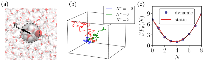
Figure 1: (a) Simulation snapshot of a small spherical observation volume, $v$, of radius, $R_{v}=0.3$ nm, in bulk water. The center of $v$ is pegged to the position of a dummy atom. The waters inside $v$ are shown in the space-fill representation, whereas those outside $v$ are shown in the licorice representation. (b) When a harmonic biasing potential, $U_{\kappa,N^{*}}$, is applied to waters in the dynamical observation volume, the waters in $v$ experience a biasing force, but so does the dummy atom pegged to the center of $v$. Trajectories depicting the motion of the dummy atom are shown here for three different biasing potentials. (c) The free energy, $\beta F_{v}(N)\equiv-\ln P_{v}(N)$, obtained using INDUS with a dynamical $v$, agrees well that obtained using a static $v$; moreover, $F_{v}(N)$ is parabolic (dashed line), highlighting that $P_{v}(N)$ for this small volume is Gaussian.

IV Hydrophobic Hydration: Fluctuations in Bulk Water

The free energetics of water density fluctuations, $F_{v}(N)$, in bulk water inform hydrophobic hydration. In particular, the free energetic cost of emptying $v$, corresponds to the hydration free energy, $F_{\rm hyd}$, of a purely repulsive hydrophobic solute, which has the same size and shape as $v$, i.e., $F_{\rm hyd}=F_{v}(N\to 0)$. Such idealized hydrophobic solutes, which simply exclude waters from the region they occupy, have long been used to study hydrophobic hydration and interactions because the extent to which they disrupt the proximal water structure is similar to that of real hydrophobic solutes Remsing and Patel (2015). In this section, we characterize $F_{v}(N)$ in two observation volumes in bulk water, which correspond to a small hard sphere and a repulsive n-hexadecane molecule as $N\to 0$.

IV.1 Ideal Spherical Solute

To illustrate the dynamic INDUS method, we first use it to estimate $F_{v}(N)$ in a small spherical volume in bulk water (Figure 1a). To estimate $F_{v}(N)$, we employ a dynamical observation volume of radius, $R_{v}=0.3$ nm, with its center pegged to a mobile dummy (ideal gas) atom. When a biasing potential, $U_{\kappa,N^{*}}(\tilde{N}_{v})=\frac{\kappa}{2}(\tilde{N}_{v}-N^{*})^{2}$, is applied, it gives rise to forces on the water molecules in $v$, but also on the dummy atom. Trajectories of the dummy atom for $\beta\kappa=1.12$ and select $N^{*}$-values are shown in Figure 1b; interestingly, as $N^{*}$ is decreased, and $v$ is emptied, its mobility appears to decrease as well. Following the INDUS prescription, biased simulations are then used to obtain $F_{v}(N)$ for this dynamical observation volume. As shown in Figure 1c, the fluctuations display Gaussian statistics in agreement with previous studies Hummer et al. (1996); Patel et al. (2011). The hydration free energy of the cavity that forms as $N_{v}\to 0$ (and of the corresponding hard sphere solute) is $F_{\rm hyd}=7.3~{}k_{\rm{B}}T$. Also shown in Figure 1c, are the free energetics obtained using a static observation volume, which is pegged to the center of the simulation box. As expected from the translational invariance of observation volumes in bulk water, we find that the $F_{v}(N)$-profiles obtained using the dynamic and static volumes are in excellent agreement with one another.

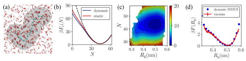
Figure 2: (a) Simulation snapshot illustrating a dynamical observation volume, $v$ (gray), in bulk water. To define $v$, we use a dummy united-atom n-hexadecane molecule (cyan); spherical sub-volumes of radius, $R_{v}=0.4$ nm, are centered on each of the united-atoms of the alkane, and $v$ is defined as the union of the 16 sub-volumes. Water molecules (red/white) inside $v$ are shown in licorice representation, whereas those outside $v$ are shown as lines. (b) The free energetics $F_{v}(N)$ of water number fluctuations in bulk water, obtained using this dynamical (flexible) $v$, are shown, and are compared to those obtained using a static (rigid) observation volume. In both cases, the statistics of water number fluctuations are Gaussian (i.e., $F_{v}(N)$ are parabolic, dashed line) near the mean of the distributions, but display fat tails for the lower $N$-values; the low-$N$ tail is fatter for the dynamical $v$. (c) Free energy, $F_{v}(N,R_{\rm g})$, is shown as a function of the number of waters, $N$, in $v$, and the the radius of gyration, $R_{\rm g}$, of the alkane; contours are drawn in increments of $1~{}k_{\rm{B}}T$. As $N$ decreases, the alkane adopts configurations with smaller $R_{\rm g}$-values. (d) The free energy $F(R_{\rm g})$ obtained by integrating $\exp[-\beta F_{v}(N,R_{\rm g})]$ over the solvent co-ordinate, $N$, agrees well the corresponding $F(R_{\rm g})$ obtained by simulating the alkane in vacuum.

IV.2 Hard-Sphere Alkane

Next, we characterize water density fluctuations in an observation volume whose shape and size can vary. The dynamical $v$ is defined as the union of 16 spherical sub-volumes; each sub-volume is pegged to a dummy united-atom of n-hexadecane, and has a radius, $R_{v}=0.4$ nm (Figure 2a). The dummy alkane chain has the same intra-molecular interactions (bonded and non-bonded) as a united-atom alkane Martin and Siepmann (1998), but its atoms do not interact with water; thus, the alkane conformational free energy landscape, which governs the size and shape of $v$, is determined entirely by the self-interactions of the alkane. We estimate the free energetics, $F_{v}(N)$, of water number fluctuations in this $v$ in bulk water using dynamic INDUS; see Figure 2b. On average, $v$ contains roughly 44 waters, and although water density fluctuations are Gaussian near the mean and at high $N$, they are enhanced at low $N$ and display marked fat tails, suggesting that the dewetting of this dynamical $v$ is co-operative Patel et al. (2012). Although our choice of $R_{v}=0.4$ nm is somewhat larger than (but close to) the hard-core radii of the alkane united-atoms, we obtain the hydration free energy of this conformationally flexible hard-sphere n-hexadecane molecule to be $\beta F_{\rm hyd}=70.4$.

To uncover the extent to which the collective dewetting of $v$ is facilitated by its conformational degrees of freedom, we additionally estimate $F_{v}(N)$ for a static observation volume defined using a representative n-hexadecane configuration. As shown in Figure 2b, although the low-$N$ fluctuations for the static $v$ are also enhanced relative to Gaussian statistics, they are suppressed relative to the dynamic $v$. The difference in estimates of $F_{v}(N\to 0)$ for the static and dynamic volumes ($78.2~{}k_{\rm{B}}T$ vs $70.4~{}k_{\rm{B}}T$), represents the difference in the hydration free energies of rigid and flexible hard-sphere alkanes ($7.8~{}k_{\rm{B}}T$). We thus find the solvation of the flexible alkane to be more favorable than that of the rigid alkane. Our findings are consistent with those of Pettitt and co-workers, who showed that the conformation of alkane chains and peptides can influence their hydration free energies substantially Harris and Pettitt (2014); Kokubo et al. (2013); Asthagiri et al. (2017). Our results also lend further support to the notion that surface-area models, which are commonly used to estimate the driving force of hydrophobic assembly, but are incapable of capturing subtle but important differences between the rigid and flexible solutes, are not appropriate for a quantitative treatment of hydrophobic hydration and interactions Harris and Pettitt (2014); Xi et al. (2017).

To further understand how the dewetting of $v$ influences the configuration of the flexible alkane (characterized using its radius of gyration, $R_{\rm g}$), we the use the dynamic INDUS simulations to estimate free energy as a function of $N$ and $R_{\rm g}$ (Figure 2c). The free energetics display a well-defined basin at $N=44$ and $R_{\rm g}=0.5$ nm. At the highest values of $N$, when $v$ is filled with waters, the alkane is extended, and displays a high value of $R_{\rm g}$. In contrast, at low values of $N$, the alkane collapses onto itself as much as possible to minimize the cost of emptying $v$. With the alkane collapsed to $R_{\rm g}=0.32$ nm, roughly 30 waters still remain in $v$. These remaining waters are then displaced with little change in $R_{\rm g}$ to bring about the complete drying of $v$. Because the system has no alkane-water interactions, integrating out the solvent degrees of freedom (represented by $N$) ought to give rise to the same configurational landscape, $F(R_{\rm g})$, that would be obtained by simulating the alkane in vacuum; this is indeed the case, as illustrated by the excellent agreement between the two quantities (Figure 2d).

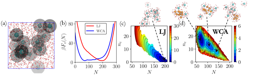
Figure 3: (a) Simulation snapshot of the system shows 13 united-atom methanes (cyan) solvated in water (red/white lines). The observation volume $v$ is defined as the union of spherical sub-volumes (gray) of radii, $R_{v}=0.5$ nm, that are centered on each of the methanes. (b) The free energy, $F_{v}(N)$, is shown for both attractive (LJ) and purely repulsive (WCA) methanes. The LJ solutes are well-hydrated, whereas the WCA solutes are not. (c, d) The free energy landscape as a function of the number, $N$, of waters in $v$, and the number, $n_{\rm c}$, of solute-solute contacts is shown for the LJ (c) and WCA (d) methanes. Methane molecules that participate in contacts are shown in orange, whereas hydrated methanes are colored cyan. Only the water molecules in $v$, i.e., waters within 0.5 nm of any methane molecules, are shown (in red/white); the remainder of the waters are hidden. For both the LJ and WCA solutes, an increase in $N$ is correlated with a corresponding decrease in $n_{\rm c}$ for $80<N<200$ and $0<n_{\rm c}<15$; the LJ solutes have a preference for being hydrated and dispersed, whereas the WCA solutes prefer to dewet and cluster.

V Hydrophobic Assembly

Hydrophobic solutes solvated in water disrupt the favorable hydrogen bonding interactions between water molecules. To minimize this disruption of favorable water-water interactions, hydrophobic solutes tend to self-assemble, forming the basis for diverse processes, ranging from supramolecular chemistry to protein folding Tang et al. (2017); Dill and MacCallum (2012). Here we use dynamic INDUS to elucidate the role of water density fluctuations in the assembly of small, hydrophobic solutes. In contrast with the previous section, where we employed dummy atoms to define $v$, and characterized $F_{v}(N)$ in bulk water, here we will make use of real hydrophobic solutes to define $v$, and characterize $F_{v}(N)$ in their hydration shells.

V.1 Role of Solute-Water Attractions

Idealized, purely repulsive solutes, which simply exclude water, have long been used to study hydrophobic effects. Such solutes themselves do not attract each other, but are driven by the solvent to aggregate in aqueous solution Pratt and Chandler (1977); Ashbaugh and Pratt (2006); Chaudhari et al. (2013); Gao et al. (2018). In addition to excluding water, real non-polar solutes also possess favorable dispersive interactions with water. Such solute-water attractive interactions offset the penalty associated with the disruption of water structure somewhat, and lower the driving force for hydrophobic assembly by stabilizing dispersed states. Indeed, the driving force for the aqueous association of two small non-polar solutes (e.g., methanes) tends to be smaller than the thermal energy.

To elucidate the role of water in the assembly of small hydrophobic solutes, and uncover how the driving force for assembly is influenced by solute-water interactions, here we study the assembly of 13 methane molecules with and without attractive interactions. Spherical sub-volumes of radii, $R_{v}=0.5$ nm are pegged to each of the methanes, and the union of these sub-volumes is chosen to be our dynamical observation volume, $v$ (Figure 3a). The observation volume thus represents the collective hydration shell of all the methanes. In Figure 3b, the free energetics of water number fluctuations in $v$ are shown for both the attractive (LJ) and purely repulsive (WCA) solutes. We find that the attractive solutes tend to be well-hydrated, with a total of nearly 200 waters being observed in their hydration shells on average. In contrast, for the repulsive solutes only about 70 waters populate $v$ on average.

To characterize the configurations that give rise to this behavior, we estimate the joint free energy, $F(N,n_{\rm c})$, where $n_{\rm c}$ is the number of solute-solute contacts, which are said to have formed when the centers of two solutes are separated by less than 0.45 nm. As shown in Figure 3c, in their lowest free energy configurations, the attractive solutes are well-hydrated, and make few solute-solute contacts. The loss of waters from $v$ is accompanied by the formation of solute-solute contacts, with the decrease in $N$ being correlated with the increase in $n_{\rm c}$ over $80<N<200$ and $0<n_{\rm c}<15$. In contrast, the stable basin in $F(N,n_{\rm c})$ for the repulsive solutes corresponds to small $N$ and large $n_{\rm c}$ (Figure 3d), i.e., the repulsive solutes prefer to cluster with the corresponding $v$ being relatively devoid of waters. Nevertheless, as with the attractive solutes, $N$ and $n_{\rm c}$ are correlated over $80<N<200$ and $0<n_{\rm c}<15$ for the repulsive solutes. Interestingly, a number of distinct metastable basins are also seen in Figure 3d for the repulsive solutes highlighting the presence of desolvation barriers that are characteristic of hydrophobic assembly.

For both the LJ and WCA methanes, once roughly 15 contacts are formed between the solutes, a further decrease in $N$ (below 80) does not lead to an increase in $n_{\rm c}$; instead the sharp increase in $F_{v}(N)$ upon decreasing $N$ below 80 waters (Figure 3b) corresponds to the dewetting of the cluster. The sharp increase in $F_{v}(N)$ seen when $N$ is increased above 200 waters, on the other hand, corresponds to excess waters being squeezed into the hydration shells of individual solutes. In the intermediate region from roughly 80 to 200 waters, $F_{v}(N)$ captures the free energetics of the correlated aggregation and dewetting (or equivalently, dissociation and hydration) of the small, hydrophobic solutes. Although the aggregation of WCA solutes is favorable ($\Delta F_{\rm agg}\approx-7~{}k_{\rm{B}}T$) and that of the LJ solutes is not ($\Delta F_{\rm agg}\approx 20~{}k_{\rm{B}}T$), in both cases, these overall preferences arise from a competition between the strong inherent tendency for the hydrophobic solutes to cluster in water (favorable), and a substantial loss of mixing entropy upon aggregation (unfavorable). For our simulations, which have 13 solutes in 868 waters, the ideal solution contribution to the loss of mixing entropy is roughly $60~{}k_{\rm{B}}T$. The inherent preference for clustering can then be quantified using the excess aggregation free energy, which is $\Delta F_{\rm agg}^{\rm ex}\approx-67~{}k_{\rm{B}}T$ for the WCA solutes and $\Delta F_{\rm agg}^{\rm ex}\approx-40~{}k_{\rm{B}}T$ for the LJ solutes.

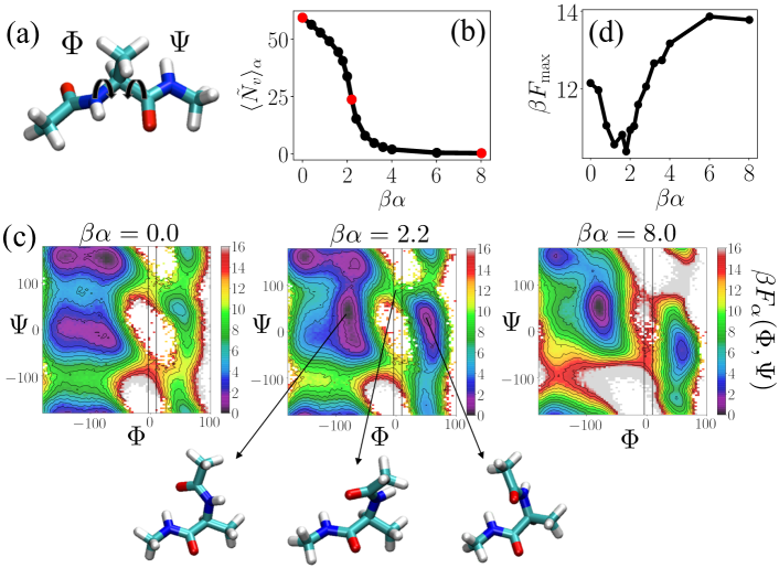
Figure 4: (a) Alanine dipeptide is shown in licorice representation along with its two principal dihedral angles, $\Phi$ and $\Psi$; the color scheme is: cyan = C, white = H, red = O, blue = N. (b) The response of the average number of waters, $\langle\tilde{N}_{v}\rangle_{\alpha}$, in the peptide hydration shell, $v$, to an unfavorable biasing potential, $\alpha\tilde{N}_{v}$, is shown as a function of the potential strength, $\alpha$. As $\alpha$ is increased, waters are systematically displaced from the peptide hydration shell. (c) The conformation free energy landscape of the peptide, $\beta F_{\alpha}(\Phi,\Psi)$, in the presence of the unfavorable potential is shown for three value of the potential strength, $\beta\alpha=0,2.2$, and $8$. Snapshots of alanine dipeptide in select basins are also shown. (d) The free energy barrier, $F_{\rm max}$, obtained by integrating $\exp[-\beta F_{\alpha}(\Phi,\Psi)]$ over $\Phi$ for $-4\leq\Phi\leq 10$ degrees and all $\Psi$ is shown as a function of $\alpha$. $F_{\rm max}$ corresponds to the barrier for transitioning between right- and left-handed turns, and is the lowest at $\beta\alpha\approx 2$ when the peptide hydration shell is roughly half empty.

VI How the Hydration of a Flexible Solute Influences its Conformation

The conformational landscape of a flexible solute arises from an interplay between its intra-molecular interactions, and its interactions with the solvent Sheng et al. (1994); Lin et al. (2014). Consequently, as the hydration of a flexible solute is varied, and the balance between intramolecular and solute-water interactions is modulated, a change in solute conformation can be triggered Athawale et al. (2007); Goel et al. (2008); Rodríguez-Ropero et al. (2015). We now illustrate the use of dynamic INDUS to characterize how the hydration of a prototypical flexible solute influences its conformational landscape.

VI.1 Alanine Dipeptide

Peptides represent a versatile template for diverse biological and materials applications Cheng et al. (1999); Shell (2010); Zerze et al. (2015). In a first step towards understanding how the conformational ensemble of a peptide is modulated by its hydration, here we study alanine dipeptide using dynamic INDUS. Alanine dipeptide has been extensively studied using molecular simulations Deng et al. (2015); Chekmarev et al. (2004), and often serves as a test-bed for enhanced sampling techniques. Although the conformational free energy landscape of alanine dipeptide can be described using only its two backbone torsional angles, $\Phi$ and $\Psi$ (Figure 4a), the landscape, $F(\Phi,\Psi)$, captures many of the relevant conformations and transitions that occur in much larger peptides and proteins.

To modulate the hydration of alanine dipeptide using dynamic INDUS, we employ an observation volume that encompasses the first hydration shell of the peptide; $v$ is defined as the union of spherical sub-volumes of radius, $R_{v}=0.6$ nm, that are centered on each of the 10 peptide heavy atoms. We then apply an unfavorable potential, $\alpha\tilde{N}_{v}$. As the strength of the potential, $\alpha$, is increased, water is systematically displaced from $v$, resulting in a decrease in the average number of waters in $v$ (Figure 4b). For each $\alpha$, we then use umbrella sampling to estimate the peptide conformational free energy landscape, $F_{\alpha}(\Phi,\Psi)$. In Figure 4c, we plot $F_{\alpha}(\Phi,\Psi)$ for three select values of $\beta\alpha=0,2.2$, and $8$, which correspond respectively to the peptide being fully hydrated, having roughly half its hydration waters, and being almost completely dewetted. For $\beta\alpha=0$, $F_{\alpha}(\Phi,\Psi)$ represents the landscape of the hydrated alanine dipeptide, whereas for $\beta\alpha=8$, $F_{\alpha}(\Phi,\Psi)$ corresponds closely to the landscape of the peptide in vacuum. As such, these landscapes display a number of well-characterized basins, which have discussed in detail elsewhere Deng et al. (2015); Chekmarev et al. (2004).

Although relatively small barriers ($\lesssim 5k_{\rm{B}}T$) must be overcome for transitions between most basins, a high free energy region ($\gtrsim 10k_{\rm{B}}T$) in the vicinity of $\Phi=0$ must be crossed to transition between a basin with $\Phi<0$ and one with $\Phi>0$. In Figure 4c, we also show simulation snapshots of alanine dipeptide in individual basins, which are called $\alpha_{\rm{R}}$ ($\Phi<0$) and $\alpha_{\rm{L}}$ ($\Phi>0$), and are populated by right- and left-handed helices, respectively. These snapshots along with a snapshot from the barrier region ($\Phi\approx 0$) collectively highlight how the alanine dipeptide molecule rotates with increasing $\Phi$, as it transitions from a right-handed to a left-handed turn. We find that the barrier height for transitioning between the turns is higher for the nearly dewetted peptide ($\beta\alpha=8$) than it is for the full hydrated peptide ($\beta\alpha=0$). Interestingly, at intermediate hydration levels, the barrier appears to be lower than at $\beta\alpha=0$ or $\beta\alpha=8$. To further investigate how the barrier height varies with hydration, we obtain estimates for the barrier free energy, $F_{\rm max}$, as a function of $\alpha$ by integrating $\exp[-\beta F_{\alpha}(\Phi,\Psi)]$ over the entire range of $\Psi$-values, and over $\Phi$ for $-4\leq\Phi\leq 10$ degrees; the range of integration is highlighted using rectangular boxes in Figure 4c. In Figure 4d, $\beta F_{\rm max}$ thus obtained is shown as a function of $\beta\alpha$, and confirms that there is an optimal hydration level that corresponds to the lowest barrier for transitioning between the right- and left-handed turns. Our results thus highlight that the barrier is the lowest for a partially hydrated peptide, and suggest that a transition between the two turns may proceed through coupled fluctuations in the hydration of the peptide and its conformation. They also suggest that the peptide may be able to transition more readily in environments that can facilitate the partial dewetting of its hydration shell, e.g., hydrophobic surfaces or confinement Anand et al. (2010); Vembanur et al. (2013); Zerze et al. (2015).

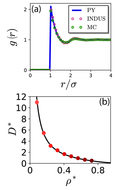
Figure 5: (a) The radial distribution function, $g(r)$, for the mimic hard sphere system with a reduced density, $\rho^{*}=0.484$, was obtained using dynamic INDUS, and is found to be in good agreement with the $g(r)$ of a true hard sphere fluid obtained from Monte Carlo simulations and the corrected Percus-Yevick equation Verlet and Weis (1972). (b) The dependence of the reduced diffusion coefficient, $D^{*}$, on the reduced density, $\rho^{*}$, obtained using dynamic INDUS simulations of mimic hard spheres (symbols) is in agreement with the empirical relation of Speedy (Equation 14) Speedy (1987).

VII Mimic Hard Sphere Systems

When the center of a spherical $v$ of radius $R_{v}$ is pegged to an ideal (non-interacting) particle, and a sufficiently strong unfavorable biasing potential is applied to the water molecules in $v$, waters are excluded from $v$, and configurations with $N_{v}=0$ are obtained; that is, the ideal particle pegged to the center of $v$ has nucleated a cavity (or a hard sphere) of radius, $R_{v}$. If several such ideal particles are introduced in the system, each with its own (independent) unfavorable biasing potential, which excludes not just waters, but also other ideal particles, a mixture of hard spheres (HS) and water can be obtained. In the limit that the system only contains such ideal particles and no waters, it mimics a HS fluid. To be precise, such a system corresponds to a soft analogue of a regularized HS fluid; configurations with $N_{v}>0$ carry an energetic penalty that is high, but not infinite.

To mimic a HS system as described above, and to characterize its dynamic properties, here we employ $M=1000$ ideal particles, which interact with one another only through the INDUS potential. The system Hamiltonian is:

$$\mathcal{H}(\{\mathbf{r}_{i}\})=\sum_{i=1}^{M}\frac{\kappa}{2}(\tilde{N}_{i}-N^{*})^{2},$$

where $\tilde{N}_{i}$ is the coarse-grained number of particles in a spherical observation volume, $v_{i}$, which is centered on particle $i$, and has a radius of $R_{v}=0.3$ nm. The INDUS potential parameters were chosen to be $\kappa=1$ kJ/mol and $N^{*}=-10$. The smoothed indicator functions were chosen to have a width of $\sigma=0.01$ nm and are cutoff at $r_{\rm c}=0.03$ nm. As long as initial configurations were chosen without any overlap, these parameters were sufficient to exclude all particles $j\neq i$ from $v_{i}$ for all $i$ in all the configurations that were sampled.

We first characterize the structure of this mimic HS fluid by estimating its radial distribution function, $g(r)$, for a system with a reduced density $\rho^{*}\equiv\rho d^{3}=0.484$, where $\rho=M/V$ is the particle density, $V$ is the volume of the simulation box, and $d$ is the effective HS diameter. To approximate $d$ for these particles, we consider the effect of the biasing potential in the limit of pairwise interactions, and use the corresponding pair potential, $u_{0}(r)$, between two particles as Andersen et al. (1971); Weeks et al. (1971); Remsing and Weeks (2013)

$$d=\int_{0}^{\infty}dr\left[1-e^{-\beta u_{0}(r)}\right].$$ (13)

This procedure yields $d=0.3166$ nm, which is slightly greater than $R_{v}=0.3$ nm. The radial distribution function, shown in Figure 5a, displays good agreement with the $g(r)$ of a true HS fluid obtained from a Monte Carlo simulation, as well as the $g(r)$ predicted by the corrected Percus-Yevick equation of Verlet and Weis Verlet and Weis (1972).

Because our mimic HS system is studied using MD simulations, we can readily estimate the diffusion coefficient of the mimic hard spheres by fitting the long time behavior of the mean squared displacement to a straight line, following the Einstein relation: $D=\lim_{t\rightarrow\infty}\left<\left|\mathbf{r}_{i}(t)-\mathbf{r}_{i}(0)\right|^{2}\right>/6t$, where $\mathbf{r}_{i}(t)$ is the position of particle $i$ at time $t$. In this way, we estimate diffusion coefficients, $D$, for mimic HS systems with varying densities. As shown in Figure 5b, as particle density is increased, the diffusion coefficients decrease, as expected for HS systems. We also compare our estimated dependence of $D$ on $\rho$ to the empirical function proposed by Speedy Speedy (1987) for HS fluids,

$$D^{*}\equiv\frac{D}{D_{0}}=\frac{1}{\rho^{*}}\bigg{(}1-\frac{\rho^{*}}{1.09}\bigg{)}(1+0.4\rho^{*2}-0.83\rho^{*4}),$$ (14)

where

$$D_{0}=\frac{3}{8}\left(\frac{k_{\rm{B}}Td^{2}}{\pi m}\right)^{1/2}$$ (15)

pertains to the zero density limit of the diffusion coefficient and $m$ is the mass of a HS particle. As shown in Figure 5b, the behavior of $D^{*}(\rho^{*})$ for our mimic HS system is in excellent agreement with Equation 14, suggesting that the dynamics of a true HS fluid are well-described by our mimic HS system. Such a correspondence between soft and hard sphere systems follows from the WCA picture of simple liquid structure Weeks et al. (1971), and has also been used to accurately predict transport properties of simple liquids Chandler (1974).

Although we have used dynamic INDUS to mimic hard sphere systems here, rhe above approach can also be used to mimic other systems with discrete potentials, such as a square well fluid. This can be accomplished by combining unfavorable particle-excluding INDUS potentials at one length scale ($R_{v}$) with favorable interactions that act on another, larger length scale, $\lambda R_{v}~{}(\lambda>1)$; i.e., in addition to having particles excluded from a hard-core region, their presence could be favored in a second observation volume that serves as the attractive region Remsing and Patel (2015).

VIII Conclusions and Outlook

The statistics of solvent density fluctuations play a central role in collective solvent-mediated phenomena, including the important class of processes that are driven by hydrophobic effects. The Indirect Umbrella Sampling (INDUS) method, which was developed to characterize such solvent fluctuations in observation volumes of all shapes and sizes, has led to numerous insights on hydrophobic hydration and interactions. However, within the INDUS framework, the positions of the observation volumes of interest as well as their shapes must be specified a priori, and must remain static throughout the biased simulations. As a result, it is not possible to use INDUS for characterizing the role of solvent fluctuations in dynamic processes, such as self-assembly or conformational change. To address this challenge, here we generalize the INDUS method to sample solvent density fluctuations in dynamical observation volumes whose positions and shapes can evolve. We focus primarily on observation volumes that are spherical or unions of spherical sub-volumes; however, the approach presented here is fairly general, and the underlying ideas can be extended to volumes of other shapes, such as cuboids or cylinders, as well as unions and intersections of such sub-volumes.

In addition to outlining the methodological framework for generalizing INDUS to dynamical volumes, we also highlight the utility of the dynamic INDUS method using a number of illustrative examples. First, we characterize the free energetics of water density fluctuations in dynamical volumes in bulk water using dummy particles to define $v$. We find that it is easier to dewet a flexible (dynamic) oligomeric volume than it is to dewet the corresponding rigid (static) volume. Next, we define the dynamical $v$ using real particles, which enables us to probe the hydration shells of these particles as they move with respect to one another. By defining $v$ to be the union of the hydration shells of several methane molecules, we are able capture the role of water in the association of these methanes. We study both purely repulsive methanes and those with dispersive attractions, and find that in both cases, there is a strong correlation between desolvation and assembly. Although we use dynamic INDUS to study the assembly of small hydrophobes, the method itself is fairly general, and could be used to study diverse assemblies, ranging from micelle formation to protein interactions. Moreover, because desolvation barriers hinder diverse self-assemblies driven by hydrophobic interactions Sharma and Debenedetti (2012, 2012); Vembanur et al. (2013); Remsing et al. (2015), the dynamic INDUS method will also facilitate the enhanced sampling of such assemblies by allowing for the biasing of the relevant (slow) solvent co-ordinates.

An important manifestation of the hydrophobic effect is solvent-mediated conformation change, such as seen in the the folding of proteins or the collapse of hydrophobic polymers in water Miller et al. (2007). Here we illustrate explore the coupling between the hydration and the conformational preferences of alanine dipeptide by defining $v$ to be the dynamically evolving hydration shell of the peptide. Interestingly, we find that the transition between right- and left-handed turns has the lowest barrier when the peptide is partially dehydrated. Although the free energetic landscapes of many conformationally flexible molecules have been extensively characterized using enhanced sampling methods, previous studies have averaged over the solvent degrees of freedom to obtain free energy as a function of conformational order parameters, such as $R_{\rm g}$ or dihedral angles Athawale et al. (2007); Goel et al. (2008); Deng et al. (2015); Chekmarev et al. (2004). The resulting loss of information makes it challenging to anticipate how the solute conformational landscape will respond to perturbations, such as proximity to interfaces or the addition of co-solutes. By providing a framework for characterizing the free energetics of solvent fluctuations in the solvation shells of conformationally flexible solutes, we hope that our work will lead to a better understanding of the interplay between solvation and conformation for diverse classes of flexible molecules, ranging from peptides and peptido-mimics to polymers and unstructured regions of proteins. We hope that the dynamic INDUS framework will also stimulate the development of sophisticated coarse-grained models Lei et al. (2015); Foley et al. (2015); Sanyal and Shell (2016); Saunders et al. (2013), which retain not only the essential solute degrees of freedom, but also the slow solvent co-ordinate degrees of freedom.

Finally, we illustrate how the dynamic INDUS method can be used to mimic hard particle systems. We use the method to simulate the dynamics of nearly-hard spheres using MD simulations, and estimate the corresponding diffusion coefficients. The ideas underlying this approach could also be extended to particles that interact via square-well potentials, thereby enabling inclusion of discrete attractive interactions Remsing and Patel (2015). By using collections of dummy particles to define $v$, it may also be possible to simulate the dynamics of non-spherical pseudo-hard particles with other shapes, such as rods or tetrahedra.