Sensitivity of nuclear statistical equilibrium to nuclear uncertainties during stellar core collapse

Abstract

I have systematically investigated the equations of state (EOSs) in nuclear statistical equilibrium under thermodynamic conditions relevant for core collapse of massive stars by varying the bulk properties of nuclear matter, the mass data for neutron-rich nuclei, and the finite-temperature modifications of the nuclear model. It is found that the temperature dependence of the nuclear free energies has a significant impact on the entropy and nuclear composition, which affect the dynamics of core-collapse supernovae. There is a little influence from the bulk properties and the mass data. For all models, common nuclei that are likely to contribute to core-deleptonization are those near $Z\approx 30$ and $N\approx 50$. A model with a semi-empirical expression for internal degrees of freedom, however, overestimates the number densities of magic nuclei with $N\approx 50$ and $82$, while a model, in which nuclear shell effects are not considered, underestimates the number densities of heavy nuclei, and especially of the magic nuclei. Other models, which include the temperature dependence of shell effects in the internal degrees of freedom and/or in the nuclear internal free energy, indicate that the difference in population between magic nuclei and non-magic nuclei disappears as the temperature increases. The construction of complete statistical EOS will require further theoretical and experimental studies of medium-mass, neutron-rich nuclei with proton numbers 25–45 and neutron numbers 40–85.

I Introduction

Hot, dense stellar matter appears in explosive astrophysical phenomena such as core-collapse supernovae and neutron-star mergers, but its equation of State (EOS) and weak-interaction rates are not well understood. The EOS determines the thermodynamic quantities and composition in terms of nucleons and various nuclei, as functions of temperature, density, and charge fraction. In the near future, gravitational waves from neutron-star mergers may provide us with information about thermodynamic quantities such as pressure at supranuclear density et al. (2017); Shibata et al. (2017). In contrast, neutrinos from core-collapse supernova may enable investigations of the nuclear composition of the EOS and the weak interaction rates at subnuclear densities.

Nuclear electron captures and coherent neutrino-nucleus scattering during the collapse of a massive star play important roles in supernova dynamics and neutrino observations. In particular, the evolution of the charge fraction and entropy in the collapsing core is very sensitive to weak interactions involving nuclei that appear at densities of $\rho_{B}\approx 10^{11}\textrm{--}10^{12}$ g/cm³ immediately before the onset of neutrino trapping. As a result, the nuclear weak interactions potentially affect the total mass of a newborn neutron star, the peak neutrino luminosity, and the strength of a shock wave Sullivan et al. (2016). Recently, some groups have suggested that medium-mass, neutron-rich nuclei may dominate the deleptonization process Sullivan et al. (2016); Furusawa et al. (2017a); Raduta et al. (2016, 2017); Titus et al. (2018), although the approach used to determine the nuclear composition or the nuclear model in the EOS differs from group to group.

Several investigations have compared different EOS models Buyukcizmeci et al. (2013); Hempel et al. (2015); Oertel et al. (2017) but have not been systematic in their approaches; therefore, it is difficult to obtain quantitative conclusions. Many research groups have already compared modern statistical EOSs that include full ensemble of nuclei, and classical single-nucleus EOSs in that a representative nucleus is used. The latter have been shown to exhibit defects Burrows and Lattimer (1984); Souza et al. (2009); Gulminelli and Raduta (2015); Furusawa et al. (2017a); Furusawa and Mishustin (2017); accordingly, this study focuses only on the former in this work. The main inputs for the statistical EOSs are experimental data and theoretical estimations for uniform nuclear matter, nuclear masses, and nuclear excitations, which are related to each other.

Bulk properties, such as incompressibility, characterize uniform nuclear matter, and their roles in supernovae have been discussed previously, with the primary focus being the stiffness of nuclear matter around nuclear densities. It is known that softer bulk properties lead to faster contractions of proto-neutron stars, higher neutrino luminosities, and the generation of more acoustic waves, resulting in more energetic explosions (see, e.g., Refs. Suwa et al. (2013); Nagakura et al. (2018a)). Most supernova EOSs employ relativistic mean-field calculations Hempel and Schaffner-Bielich (2010); Typel et al. (2010); Furusawa et al. (2011, 2013); Furusawa et al. (2017b); Shen et al. (2011, 2011); Steiner et al. (2013) or Skrme-type interactions Schneider et al. (2017), using fixed parameter sets. Recently, some realistic nuclear EOSs based on a variational method that employs the bare nuclear potentials have also been presented Togashi et al. (2017); Furusawa et al. (2017c).

Nuclear masses are another essential ingredient for the statistical EOSs as the nuclear composition at low densities and temperatures is sensitive to the nuclear binding energies. During core collapse, not only do nuclei close to the stability line appear but so do extremely heavy and/or neutron-rich nuclei; we require theoretical mass data for such nuclei. Blinnikov et al. Blinnikov et al. (2011) and the FYSS EOSs Furusawa et al. (2011, 2013); Furusawa et al. (2017b) utilize the KTUY mass data Koura et al. (2005), whereas the SHO EOS Shen et al. (2011, 2011) adopts the old version of FRDM Moller et al. (1995). In addition, the authors of the HS EOSs Hempel and Schaffner-Bielich (2010); Steiner et al. (2013) have prepared various EOSs based on different theoretical mass data; see, e.g., Refs. Geng et al. (2005); Moller et al. (1995); Roca-Maza and Piekarewicz (2008); Lalazissis et al. (1999).

At finite temperatures, nuclear excitations must be included in the EOS. They increase the internal degrees of freedom, especially for large and non-magic nuclei, which have nucleons in open-shells. Ideally, in the statistics, we should precisely count all the states with individual excitation energies, for all nuclei; however, experimental data for the nuclear level densities are insufficient. In addition, theoretical calculations, such as shell-model calculation Tsunoda et al. (2017), for all states would be quite difficult. For now, we employ two approaches to take account of the finite-temperature effects. One introduces internal partition functions as a function of temperature in determining the number densities of nuclei. The other approach phenomenologically represents the ground state and all excited states by a hot nucleus so that the nuclear internal free energy depends on the temperature and is identical to nuclear mass at zero temperature.

The former approach allows us to partly use the experimental data on level densities directly if the temperature is not too high and the excitations are weak. Ishizuka et al. Ishizuka et al. (2003) and the HS EOS employ a semi-empirical expression for internal partition functions provided by Fai and Randrup Fái and Randrup (1982), which depends only on the temperature and mass number. The SRO EOS Schneider et al. (2017) utilizes tabulated partition functions provided by Raucher Rauscher et al. (1997); Rauscher and Thielemann (2000); Rauscher (2003), which is based on a Fermi-gas approach, using experimental data for level densities and the FRDM mass data Moller et al. (1995) to evaluate the separation energies of nucleons. The latter approach employs a temperature-dependent internal free energy, such as in the SMSM (statistical model for supernova matter) EOS Botvina and Mishustin (2004, 2010); Buyukcizmeci et al. (2014). The SMSM EOS is an extension of the SMM (statistical multifragmentation model) EOS Bondorf et al. (1995), which reproduces fragmentations in low-energy heavy-ion collisions. The SHO EOS also assumes similar excitation effects for the bulk free energy of the nuclei. This approach may be valid for reproducing the ensemble of hot nuclei when the temperature is sufficiently high to make the excited states dominant. Ground-state properties, such as neutron magic numbers and pair energies, are considered to be almost washed out at $T\approx$ 2–3 MeV Brack and Quentin (1974); Bohr and Mottelson (1998); Sandulescu et al. (1997); Nishimura and Takano (2014), which are temperatures typical of the late phases of core collapse. The FYSS EOS Furusawa et al. (2017b, c) employs temperature interpolation between the internal free energies of cold and hot nuclei.

In the present work, I investigate the sensitivity of the nuclear composition to several nuclear uncertainties, the bulk properties of nuclear matter, the nuclear mass data, and the finite-temperature modeling in order to clarify ambiguities in the supernova EOS at subnuclear densities and to organize the target properties and nuclides for future theoretical and experimental studies. The organization of this paper is as follows: In Sec. II, I describe the formulations and inputs for the EOSs. Comparisons among EOSs under thermodynamics conditions during core collapse of massive 15M_⊙ and 25M_⊙ stars are discussed in Sec. III. Finally, a summary is given in Sec. IV

II Nuclear physics inputs for statistical equations of state

The free-energy density is minimized with respect to the number densities of all particles, subject to the constrains of baryon and charge conservation, to obtain the EOS as a function of the volume-averaged values of the baryon number density $n_{B}$, temperature $T$, and charge fraction $Y_{p}$. I systematically change three ingredients and Table 1 summarizes the specific cases. Below, I explain the 14 models— 1B, 1D, 1E, 2FB, 2FD, 2FE, 2HE, 2KE, 2WE, 3FE, 3HE, 3KE, 3WE, and 4FE —for which the number and abbreviations denote, in order, the treatment of finite-temperature effects for nuclear excitations, the choice of mass data for models 2–4, and the parameter set for bulk nuclear matter.

The constituents of nuclear matter under nuclear statistical equilibrium are the dripped nucleons and all nuclei. The free-energy density can be given by

$$f=\xi\left[n^{\prime}_{p}m_{p}+n^{\prime}_{n}m_{n}+(n^{\prime}_{p}+n^{\prime}_{n})\omega\left(n^{\prime}_{p}+n^{\prime}_{n},T,\frac{n^{\prime}_{p}}{n^{\prime}_{p}+n^{\prime}_{n}}\right)\right]$$

$$+\sum_{AZ}n_{AZ}\left\{T\left[\ln\left(\frac{n_{AZ}/\kappa}{g_{AZ}(M_{AZ}T/2\pi\hbar^{2})^{3/2}}\right)-1\right]+M_{AZ}\right\},$$ (1)

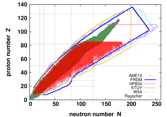
Figure 1: Nuclear species for which experimental nuclear mass data AME12 Audi et al. (2012) (green crosses) have been adopted. Theoretical mass data are available in extended regions in the (N, Z) plane inside the following contours: FRDM Möller et al. (2016) (blue solid line), HFB24 Goriely et al. (2013) (magenta dotted line), KTUY Koura et al. (2005) (orange dashed line), and WS4 Wang et al. (2014) (cyan double-dotted line). The red circles indicate nuclei for which the data are obtained from Rauscher’s partition function Rauscher (2003). The black dashed lines denote the neutron- and proton-magic numbers.

where $n^{\prime}_{p}$ and $n^{\prime}_{n}$ are the local number densities of protons and neutrons, respectively, and $m_{p}$ and $m_{n}$, are the corresponding masses Furusawa and Mishustin (2018). The volume factor for free nucleons is defined as $\xi=V^{\prime}/V$ with the vapor volume $V^{\prime}$ and the total volume $V$. The local free energy density of the dripped nucleons is obtained from a nuclear-matter calculation of $\omega(n_{B},T,x)$ as a function of the local values of $n_{B}$, $T$, and the charge fraction $x$, as in Furusawa and Mishustin Furusawa and Mishustin (2018). The vapor volume can be calculated as $V^{\prime}=V(1-\sum_{AZ}n_{AZ}A/n_{sAZ})$. The summation covers all nuclides listed in the tabulated data, theoretical mass data or partition functions, as discussed later and shown in Fig. 1. The quantities $M_{AZ}$, $g_{AZ}$, $n_{AZ}$, and $n_{sAZ}$ are the mass, internal degree of freedom, number density, and saturation density of the nucleus with the mass number $A$ and the proton number $Z$. The translational energy of the nuclei is calculated as for an ideal Boltzmann gas, with excluded volume effects represented by $\kappa=1-n_{B}/n_{0}$.

II.1 Nuclear matter calculation for dripped nucleons and bulk energies of nuclei

The bulk properties at the nuclear saturation density $n_{0}$ for symmetric matter are characterized by the following parameters: the binding energy at saturation $\omega_{0}$, the incompressibility $K_{0}$, symmetry energy at saturation $S_{0}$, and symmetry energy slope parameter $L$. I use the three parameter sets Oyamatsu and Iida (2003, 2007) listed in Tab 2. Parameters B and E share the same value of $K_{0}$, while parameters D and E are based on the same value of the saturation slope parameter $y=-K_{0}S_{0}/(3n_{0}L)$, which gives the saturation point of asymmetric nuclear matter at about $x=0.5$ as $n_{0}+(1-2x)^{2}S_{0}/y$. The parameters other than $K_{0}$ and $y$ are optimized to reproduce the masses and radii of stable nuclei by using Thomas–Fermi calculations Oyamatsu and Iida (2003, 2007). The free energy per baryon for uniform nuclear matter, $\omega(n_{B},T,x)$, is based on the finite-temperature calculation Furusawa and Mishustin (2018) of Oyamatsu and Iida Oyamatsu and Iida (2003, 2007) and is given by:

$$\omega(n_{B},T,x) = \omega_{int}+\omega_{kin},$$ (2)

$$\omega_{int} = 4x(1-x)v_{s}(n_{B})/n_{B}+(1-2x)^{2}v_{n}(n_{B})/n_{B},$$

$$\omega_{kin} = \frac{T}{2\pi^{2}n_{B}}\left(\frac{2m_{p}T}{\hbar^{2}}\right)^{3/2}F_{3/2}(\eta_{p})+\frac{T}{2\pi^{2}n_{B}}\left(\frac{2m_{n}T}{\hbar^{2}}\right)^{3/2}F_{3/2}(\eta_{n}),$$

$$v_{s}(n_{B}) = a_{1}n_{B}^{2}+\frac{a_{2}n_{B}^{3}}{1+a_{3}n_{B}},$$ (3)

$$v_{n}(n_{B}) = b_{1}n_{B}^{2}+\frac{b_{2}n_{B}^{3}}{1+b_{3}n_{B}},$$ (4)

where $\omega_{int}$ and $\omega_{kin}$ are interaction and kinetic energies, $v_{s}$ and $v_{n}$ are the energy densities for symmetric matter and pure-neutron matter, respectively, $b_{3}=$1.58632 fm³ and $\eta_{p/n}=\left[\mu^{0}_{p/n}-\partial(\omega_{int}n^{0}_{p/n})/\partial n^{0}_{p/n}\right]/T$. The number densities of protons, $xn_{B}$, and neutrons, $(1-x)n_{B}$, correspond to the chemical potentials, $\mu^{0}_{p/n}$, and $F_{k}(\eta)$ is defined by $F_{k}(\eta)=\int_{0}^{\infty}u^{k}\left[1+\exp{(u-\eta)}\right]^{-1}du$. The parameters $a_{1}$, $a_{2}$, $a_{3}$, $b_{1}$, and $b_{2}$ for the potential energies are fitted to reproduce the bulk parameters in Table 2 {see Eqs. (10–14) in Ref. Furusawa and Mishustin (2018)}.

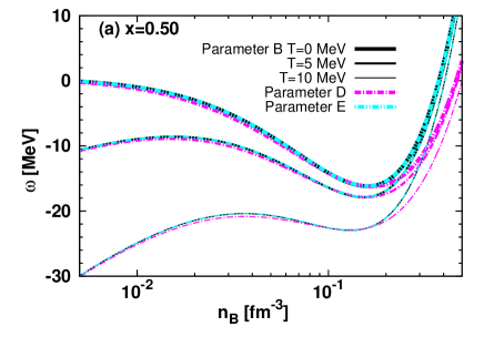
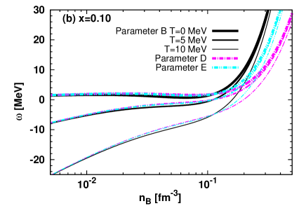
Figure 2: Free energy per baryon for symmetric nuclear matter (left panel, $x=0.5$) and for asymmetric nuclear matter (right panel, $x=0.1$) for parameter sets B (black solid lines), D (magenta dashed-dotted line), and E (cyan double-dotted dashed line) at $T=$0 MeV (thick lines), 5 MeV (medium lines), and 10 MeV (thin lines).

Figure 2 presents the free-energy densities for the three parameter sets. Differences appear at $n_{B}\approx 10^{-2}$ fm^-3. For symmetric matter with $x=0.5$, the bulk free energies for parameter sets B and E are almost identical to each other as they have the same value of $K_{0}$. In contrast, the parameter set D has the soft property of a more gradual growth of $\omega$ because of the smaller value of $K_{0}$. For asymmetric matter with $x=0.1$, the smaller values of $L$ make the densities higher, at which $\omega$ increases steeply.

II.2 Nuclear mass data and model for internal free energy

The nuclides taken into account in the statistical EOSs are presented in Fig 1. I utilize experimental mass data from AME12 Audi et al. (2012) for those nuclei with data available and theoretical nuclear mass data from FRDM Möller et al. (2016), HFB24 Goriely et al. (2013), KTUY Koura et al. (2005), or WS4 Wang et al. (2014) for the other nuclei. The middle character—F, H, K, or W—in the names of models 2-4 denotes the specific dataset. These data also optimize the surface energy parameters for model 2, as discussed later. Model 1 includes the nuclides with FRDM mass data available, although I do not use the values of nuclear masses.

In nuclear statistical equilibrium, the number densities of all nuclei are given by

$$n_{AZ}=\kappa\sum_{i}g_{AZi}\left(\frac{M_{AZ}T}{2\pi\hbar^{2}}\right)^{3/2}{\rm exp}\left(\frac{\mu_{AZ}-M_{AZ}}{T}\right),$$ (5)

where the index $i$ runs over the ground state and all excited states, $g_{AZi}$ is the degree of freedom of state $i$, $\mu_{AZ}=(A-Z)\mu_{n}+Z\mu_{p}$, and $\mu_{n}$ and $\mu_{p}$ are the chemical potentials of neutrons and protons, respectively. Unfortunately, the experimental data of the excitation energies or level densities are insufficient at present. Instead of including all excited states explicitly, we often introduce internal degrees of freedom, $g_{AZ}(T)$, and/or internal free energy, $F_{AZ}(T)$, as a function of $T$:

$$n_{AZ} \simeq \kappa g_{AZ}(T)\left(\frac{M_{AZ}T}{2\pi\hbar^{2}}\right)^{3/2}{\rm exp}\left(\frac{\mu_{AZ}-M_{AZ}}{T}\right),$$ (6)

$$\simeq \kappa g_{AZ}^{s}\left(\frac{M_{AZ}T}{2\pi\hbar^{2}}\right)^{3/2}{\rm exp}\left(\frac{\mu_{AZ}-F_{AZ}(T)}{T}\right).$$ (7)

The former equation can be obtained from the relations $\mu_{AZ}=\partial f/\partial n_{AZ}$ and Eq. (1). Models 3 and 4 employ $g_{AZ}(T)$ and use cold nuclear masses $M_{AZ}$ that include finite-density effects only, as in Eq. (6) and explained later. In the models 1 and 2, I substitute $F_{AZ}(T)$ and simplified factors $g_{AZ}^{s}$ for $M_{AZ}$ and $g_{AZ}(T)$, as in Eq. (7). For models 1B, 1D and 1E, I employ a statistical model of the SMSM EOS Botvina and Mishustin (2004, 2010); Buyukcizmeci et al. (2014) with the nuclear bulk parameters and the formulation of Coulomb energies modified. Models 2FB, 2FD, 2FE, 2HE, 2KE, and 2WE, are based on the liquid-drop model (LDM) Furusawa and Mishustin (2018) with the shell washout effect introduced in the FYSS EOS Furusawa et al. (2011, 2013); Furusawa et al. (2017b, c).

The internal free energy of model 1 with proton numbers $Z>5$ and neutron numbers $N>5$ is composed of nucleon rest masses and bulk, Coulomb, and surface energies as follows:

$$F_{AZ} = Zm_{p}+(A-Z)m_{n}+F_{AZ}^{B}+F_{AZ}^{C}+F_{AZ}^{Sf},$$ (8)

$$F_{AZ}^{B} = A\left(-\omega_{0}-\frac{T^{2}}{\epsilon}\right)+S_{0}\frac{(A-2Z)^{2}}{A},$$ (9)

$$F_{AZ}^{C} = \displaystyle{\frac{3}{5}\left(\frac{3}{4\pi}\right)^{-1/3}e^{2}n_{sAZ}^{2}\left(Z/A-n^{\prime}_{p}/n_{sAZ}\right)^{2}\left({A/n_{sAZ}}\right)^{5/3}D(u_{AZ})},$$ (10)

$$F_{AZ}^{Sf} = 18\left(\frac{T^{2}_{cAZ}-T^{2}}{T^{2}_{cAZ}+T^{2}}\right)^{5/4}A^{2/3}.$$ (11)

In Eq. (10), $D(u_{AZ})=1-\frac{3}{2}u_{AZ}^{1/3}+\frac{1}{2}u_{AZ}$, where the filling factor $u_{AZ}=(n_{e}-n^{\prime}_{p})/(Zn_{sAZ}/A-n^{\prime}_{p})$, $n_{e}(=Y_{p}n_{B})$ is the electron number density, and $e$ is the elementary charge. In the model, I ignore the iso-spin dependencies of the critical temperature for nuclear vaporization and nuclear saturation densities as $T_{cAZ}=18$ MeV and $n_{sAZ}=n_{0}$.

In model 2, I consider nuclear shell effects, $F_{AZ}^{Sh}$, and dependencies of $n_{sAZ}$ on $T$ and on $Z/A$ and employ other formulations for bulk and surface energies. The internal free energy is given by

$$F_{AZ} = Zm_{p}+(A-Z)m_{n}+F_{AZ}^{B}+F_{AZ}^{C}+F_{AZ}^{Sf}+F_{AZ}^{Sh},$$ (12)

$$F_{AZ}^{B} = A\{\omega(n_{sAZ},T,Z/A)\},$$ (13)

$$F_{AZ}^{Sf} = \left(\displaystyle{\frac{36\pi A^{2}}{n_{sAZ}^{2}}}\right)^{1/3}\sigma_{AZ}(T)\left(1-\displaystyle{\frac{n^{\prime}_{p}+n^{\prime}_{n}}{n_{sAZ}}}\right)^{2},$$ (14)

$$F_{AZ}^{Sh} = F_{AZ0}^{Sh}\displaystyle{\frac{\tau_{AZ}}{{\rm sinh}\tau_{AZ}}}.$$ (15)

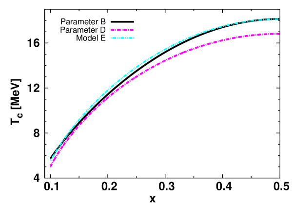
Figure 3: Critical temperatures for bulk nuclear matter, above which the bulk pressure has no local minimum, as a function of charge fraction for parameter sets B (black solid lines), D (magenta dashed-dotted line), and E (cyan double-dotted dashed line).

The quantity $F_{AZ}^{B}$ is based on the same calculations for dripped nucleons as Eq. (2), and $n_{sAZ}(T)$ is defined as the density at which the free energy, $\omega(n_{B},T,Z/A)$, takes its local minimum value around $n_{0}$. The Coulomb energy, $F_{AZ}^{C}$, is calculated by Eq. (10). For $F_{AZ}^{Sf}$ in Eq. (14), $\sigma_{AZ}(T)=\sigma_{0}[(T^{2}_{cAZ}-T^{2})/(T^{2}_{cAZ}+T^{2})]^{5/4}(16+C_{s})/[(1-Z/A)^{-3}+(Z/A)^{-3}+C_{s}]$ and $T_{cAZ}$, is defined by using the bulk pressure, $P_{bulk}=n_{B}^{2}\partial\omega(n_{B},T,x=Z/A)/\partial n_{B}$. This is the temperature at which $(\partial P_{bulk}/\partial n_{B})|_{x}=0$ and $(\partial^{2}P_{bulk}/\partial n_{B}^{2})|_{x}=0$ simultaneously and is shown in Fig. 3 for each bulk parameter set. The last factor in Eq. (15) expresses the washout effects, where $\tau_{AZ}=2\pi^{2}T/(41A^{-1/3})$ Furusawa et al. (2013); Furusawa et al. (2017b).

The shell energies of the ground states are set equal to the mass data, $M_{AZ}^{data}$, minus the LDM mass-energy in a zero-density medium, i.e., $F_{AZ0}^{Sh}=M_{AZ}^{data}-[Zm_{p}+(A-Z)m_{n}+F_{AZ}^{B}+F_{AZ}^{C}+F_{AZ}^{Sf}]_{n_{e}=0,n^{\prime}_{p}=0,n^{\prime}_{n}=0,T=0}$. This assumption allows the internal free energy of Eq. (12) to reproduce exactly the mass data at low temperatures and densities. Here, I assume the shell energy to be positive to avoid negative entropy production. Nuclear excitations usually increase the internal degrees of freedom, which corresponds to a free-energy reduction associated with a temperature increase and to positive entropy production. This assumption for the sign of shell correction, however, is not typical and, in some references Egidy and Bucurescu (2005), the shell energies of magic nuclei take negative values. The surface tension $\sigma_{0}$ and isospin-dependence parameter $C_{s}$ are optimized to minimize the total deviation of the LDM mass-energy (internal free energy in zero-temperature limit) per baryon from the mass data or the sum of the shell energies per baryon, $\sum_{Z>5,n>5}F^{Sh}_{AZ0}/A$. The resulting values of these quantities are listed in Table 1.

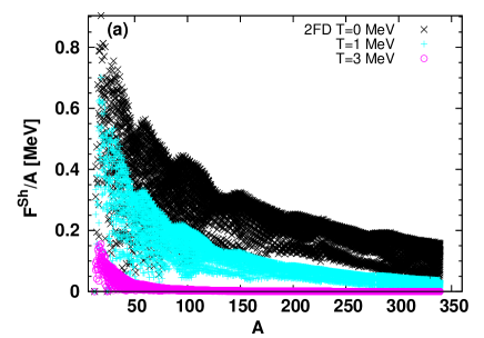
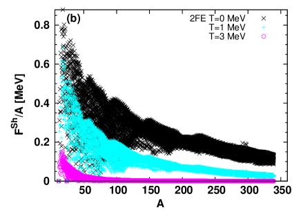
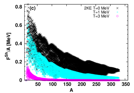
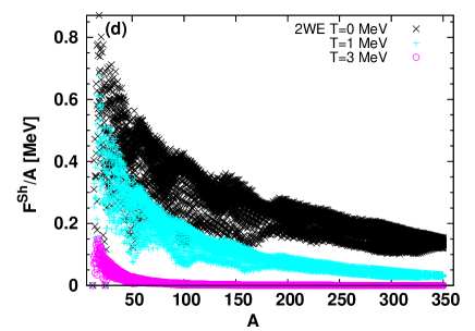
Figure 4: Shell energies per baryon for models 2FD (top-left panel), 2FE (top-right panel), 2KE (bottom-left panel), and 2WE (bottom-right panel) at $T=$0 MeV (black crosses), 1 MeV (cyan pluses), and 3 MeV (magenta circles).

Figure 4 illustrates the temperature dependence of the shell energies for models 2FD, 2FE, 2KE, and 2WE. The combination of mass data and bulk parameters leads to a set of shell energies and surface tension parameters. At $T=3$ MeV, the nuclear shell effects are significantly reduced, especially for nuclei with large mass numbers. Note that this formulation is still rough and may overestimate the shell damping as discussed later.

In models 3 and 4, the temperature dependence is encapsulated in internal degrees of freedom $g_{AZ}(T)$ as in Eq. (6). To evaluate the nuclear masses, I take into account only Coulomb screening effects: $\Delta E^{C}_{AZ}=F_{AZ}^{C}(n_{e},n^{\prime}_{p})-F_{AZ}^{C}(0,0)$ from Eq. (10), with $M_{AZ}=M_{AZ}^{data}+\Delta E^{C}_{AZ}$. In models 3 and 4, I set $n_{sAZ}=n_{0}$ for all nuclei.

II.3 Internal degrees of freedom

In model 3, I use a semi-empirical function for internal degrees of freedom that depends only on the temperature and mass number Fái and Randrup (1982). It is utilized in the HS EOSs Hempel and Schaffner-Bielich (2010); Steiner et al. (2013) and can be given by

$$g_{A}(T)=g_{A}^{0}+\frac{c_{1}}{A^{5/3}}\int_{0}^{16.2A}dEe^{-E/T}\exp\left(\sqrt{2a(A)E}\right),$$ (16)

where $a(A)=(A/8)(1-c_{2}A^{-1/3})$MeV^-1, $c_{1}=0.2$MeV^-1, $c_{2}=0.8$, and $g_{A}^{0}=1$ for even nuclei and $g_{A}^{0}=3$ for odd nuclei, and the upper bound of the integral is set to be a typical bulk energy, $16.2A$, as in the HS EOS. There are several options for the upper limit according to each model of energy integral: infinity; nuclear binding energies; the smaller of neutron and proton separation energies with in-medium modifications Gulminelli and Raduta (2015); Fowler et al. (1978). The choice of the upper bound, however, does not significantly change the results. Model 4FE employs Raucher’s tabulated data for the internal partition functions $g_{AZ}(T)$ for each nucleus Rauscher (2003), which are used in the SRO EOS Schneider et al. (2017). The nuclei listed in these data are limited, as shown in Fig 1; therefore, I assume no excitations for the nuclei, for which partition function data are unavailable, even if the mass data are available.

In models 1 and 2, I consider the excited-state contributions to the quantities of $F_{AZ}^{B}$, $F_{AZ}^{Sf}$, and $F_{AZ}^{Sh}$ in Eqs. (8) and (12). The values of $g_{AZ}^{s}$ in model 1 are set to be unity as in the original EOS. In model 2, the ground-state spin factors, $g_{AZ}^{0}$, are taken from Ref. Rauscher and Thielemann (2000) for those nuclei for which data are available and are set to $g_{AZ}^{0}=1$ for other even nuclei and $g_{AZ}^{0}=3$ for other odd nuclei. The internal degrees of freedom are assumed to be washed out according to $g_{AZ}^{s}=(g_{AZ}^{0}-1)\tau_{AZ}/{\rm sinh}\tau_{AZ}+1$, approaching unity with the reduction in the shell energy because of increase in the excited states Furusawa et al. (2017b).

For comparison with the internal degrees of freedom for models 3 and 4, I define effective internal degrees of freedom for models 1 and 2 in refer to Hempel Hempel (2010):

$$g^{*}_{AZ}(T)=g_{AZ}^{s}{\rm exp}\left(\frac{F^{0}_{AZ}-F^{*}_{AZ}}{T}\right).$$ (17)

Here, $F^{*}_{AZ}$ is the internal free energy in the zero-density-medium limit, but at finite temperature, $F_{AZ}(T)=F_{AZ}(T,n_{e}=0,n^{\prime}_{p}=0,n^{\prime}_{n}=0)$. The internal free energy in vacuum limit ($T=0$, $n_{e}=0$, $n^{\prime}_{p}=0$, and, $n^{\prime}_{n}=0$), $F^{0}_{AZ}$, is identified with $M_{AZ}^{data}$ in model 2. This formulation leads to the expression for the number density of nuclei in the zero-density-medium limit:

$$n_{AZ}(T)=g^{*}_{AZ}(T)\left(\frac{F_{AZ}^{0}T}{2\pi\hbar^{2}}\right)^{3/2}{\rm exp}\left(\frac{\mu_{AZ}-F_{AZ}^{0}}{T}\right),$$ (18)

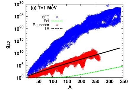
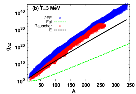
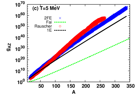
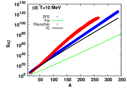
Figure 5: Effective internal degrees of freedom for all nuclei for models 1E (black dashed lines) and 2FE (blue crosses), as calculated from Eq. (17); semi-empirical expression for internal degrees of freedom as functions of mass number, as given by Eq. (16) and provided by Fai and Randrup Fái and Randrup (1982) (green dashed lines); and internal partition functions in tabular form of Raucher Rauscher (2003) (red circle dots) at $T=$1 MeV (top-left panel), 3 MeV (top-right panel), 5 MeV (bottom-left panel) and 10 MeV (bottom-right panel).

which is similar to Eq. (6) for models 3 and 4. The internal degrees of freedom for these four approaches are presented in Fig. 5. Model 1 generally agrees with Rasucher’s data (model 4) at $T=1$ MeV and tends to exhibit fewer internal degrees of freedom than model 2 at any temperature. For model 2, nuclei with small mass numbers are more likely to be excited, as compared with the other models, as their shell and surface energies per baryon are large relative to nuclei with large mass numbers. The semi-empirical internal degrees of freedom for model 3 are clearly fewer than those given by the other three models.

For all models, light clusters with $Z\leq 5$ or $N\leq 5$ are calculated as ideal Boltzmann gases using the excluded volume, $\kappa$, Coulomb screening effects, $F_{AZ}=M_{AZ}=M_{AZ}^{data}+\Delta E^{C}_{AZ}$, and no excitation, $g_{AZ}=g_{0}$ as in Ref. Furusawa and Mishustin (2018).

III nuclear statistical equilibrium in collapsing cores

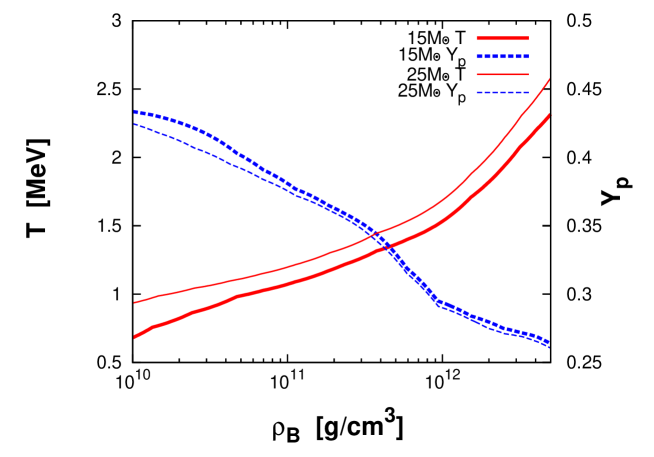
Figure 6: Temperatures (red solid lines) and charge fractions (blue dashed lines) as a function of density at the centers of the collapsing cores of supernova progenitors of 15M_⊙ (thick lines) and 25M_⊙ (thin lines) Juodagalvis et al. (2010).

I next compare some models listed in Table 1 along core-collapse trajectories for stars of 15M_⊙ and 25M_⊙ Juodagalvis et al. (2010). Figure 6 presents the temperature and charge fraction as a function of density for these supernova progenitors. The progenitor with 25M_⊙ exhibits higher temperature and lower charge fractions for the same density. Note that these quantities depend on the EOS and the results of core-deleptonization in actual core-collapse simulations, although I assume the same thermodynamic conditions for all EOSs in this comparison. I focus mainly on the nuclear composition of heavy nuclei at $\rho_{B}\approx 10^{11-12}$ g/cm³, because weak interactions involving heavy nuclei play fundamental roles in core-deleptonization immediately before neutrino sphere formation, and the impacts of nucleons and light clusters are not dominant.

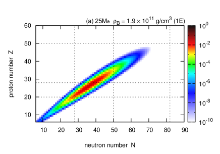
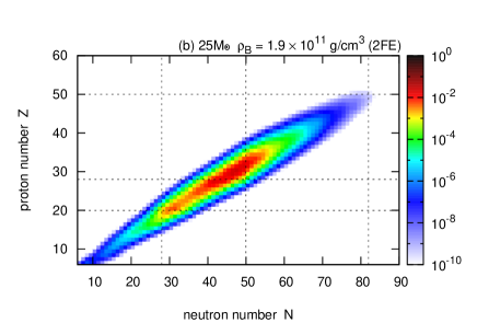
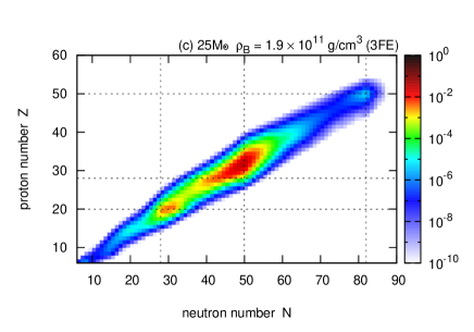
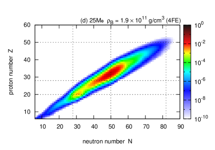
Figure 7: Mass fractions $X_{AZ}$ in the $(N,Z)$ plane at $(\rho_{B},T,Y_{p})=(1.9\times 10^{11}$ g/cm³, 1.3 MeV, 0.36) for the collapsing core of a 25M_⊙ supernova progenitor for models 1E (top-left panel), 2FE (top-right panel), 3FE (bottom-left panel), and 4FE (bottom-right panel).

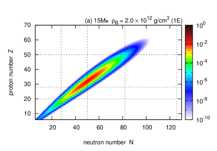
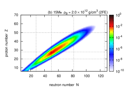
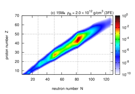
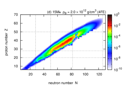
Figure 8: Mass fractions $X_{AZ}$ in the $(N,Z)$ plane at $(\rho_{B},T,Y_{p})=(2.0\times 10^{12}$ g/cm³, 1.8 MeV, 0.28) for the collapsing core of a 15M_⊙ supernova progenitor for models 1E (top-left panel), 2FE (top-right panel), 3FE (bottom-left panel), and 4FE (bottom-right panel).

Figures 7 and 8 display the mass fractions of all heavy nuclei, $X_{AZ}=An_{AZ}/n_{B}$, for models 1E, 2FE, 3FE, and 4FE under thermodynamical conditions at $(\rho_{B},T,Y_{p})=(1.9\times 10^{11}$ g/cm³, 1.3 MeV, 0.36) for the 25M_⊙-star and $(2.0\times 10^{12}$ g/cm³, 1.8 MeV, 0.28) for the 15M_⊙-star. Model 1E shows smoother mass distribution than the other models, because of the lack of nuclear shell effects. Other models generally have a monomodal or bimodal structure around neutron magic numbers ($N=$28, 50, and 82). Model 3FE assumes the semi-empirical function for internal degrees of freedom and cold nuclear mass and, as a result, overestimates the mass fractions of these magic nuclei. In model 2FE, the shell energies $F_{AZ}^{Sh}$ are washed out, and, consequently, non-magic nuclei are also abundant. In model 4FE, Rauscher’s data for the internal degrees of freedom take into account the shell effects; therefore, non-magic nuclei are more easily excited and have larger values of $g_{AZ}(T)$ than the magic nuclei. Therefore, models 2FE and 4FE produce wider and smoother distributions of nuclei with large abundances $X_{AZ}$ in the $(N,Z)$ plane than model 3FE. Unfortunately, model 4FE lacks the partition function data for some important nuclei close to the abundance peaks, e.g., $(N,Z)=(85,28)$ and (75, 35), as displayed in Fig. 1.

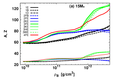
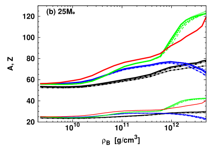
Figure 9: Average mass numbers (thick lines) and proton numbers (thin lines) at the centers of the collapsing cores of supernova progenitors of 15M_⊙ (left panel) and 25M_⊙ (right panel) for models 1B (black dashed-dotted lines), 1D (black double-dotted dashed lines), 1E (black solid lines), 2FB (blue dashed-dotted lines), 2FE (blue solid lines), 2KE (blue dashed lines), 3FE (green solid lines), 3KE (green dashed lines), 3HE (green dotted lines), 3WE (green double-dotted lines), and 4FE (red solid lines).

The average mass numbers and proton numbers of heavy nuclei are shown in Fig. 9 for almost all the models. The impact on these quantities of the mass data and bulk properties is not large, while the choice of partition function alters them greatly. The average mass numbers for models 1B, 1D, and 1E are smaller and grow more gradually than the other models owing to the lack of shell effects. For models 2FB, 2FE, and 2KE, nuclei with smaller mass numbers are more highly excited than those in the other models, as discussed above and shown in Fig. 5. Therefore, they tend to produce smaller average mass numbers than do models 3 and 4. As discussed above and displayed in Figs. 7 and 8, nuclear shell effects remain at high temperatures in model 3FE. Hence, only that model leads to a step-wise growth in the average mass numbers and proton numbers, owing to the neutron-magic numbers: at about $\rho_{B}=10^{12}$ g/cm³, the dominant constituents of nuclear matter abruptly change nuclei with $N\approx 50$ to those with $N\approx 82$.

The bulk parameter does not affect significantly the results among models 2. This is due to the internal free energies being almost equal to the mass data at low temperatures owing to the introduction of shell energies and to the parameters for nuclear bulk energies other than $K_{0}$ and $y$ and for surface tensions also being optimized to reproduce the similar nuclear properties, such as nuclear masses and radii. The differences arising from the bulk properties are more visible among models 1. The larger values of $S_{0}$ and $L$ reduce the binding energies and the average mass numbers in models 1B and 2FB compared with 1D, 1E, and 2FE. The choice of theoretical mass data does not significantly influence the results either in models 2, as nuclei for which the experimental mass data exist are dominant. Differences from the theoretical mass data appear only for neutron-rich nuclei at high temperatures, where the shell effects derived from the mass data no longer survive. Models 3FE, 3HE, 3KE, and 3WE display larger differences due to the mass data than models 2KE and 2FE, because they do not take into account the shell damping.

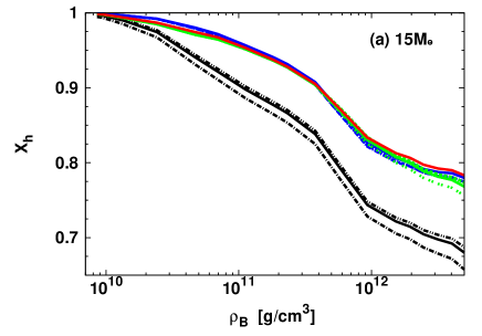
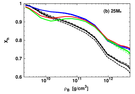
Figure 10: Total mass fractions of heavy nuclei at the centers of the collapsing cores of supernova progenitors of 15M_⊙ (left panel) and 25M_⊙ (right panel) for models 1B (black dashed-dotted lines), 1D (black double-dotted dashed lines), 1E (black solid lines), 2FB (blue dashed-dotted lines), 2FE (blue solid lines), 2KE (blue dashed lines), 3FE (green solid lines), 3KE (green dashed lines), 3HE (green dotted lines), 3WE (green double-dotted lines), and 4FE (red solid lines).

Figure 10 shows the total mass fraction of heavy nuclei, $X_{h}=\sum_{Z>5,N>5}X_{AZ}$. It is found that the mass fraction is generally large for a model that has many internal degrees of freedom. The difference is greater for the 25M_⊙ star in which the central temperature is higher than that in the 15M_⊙ star. Model 4FE always reproduces larger mass fractions than model 3FE. At the beginning of core collapse, models 2FB, 2FE, and 2KE yield larger mass fractions than models 3FE or 4FE because of the larger internal degrees of freedom, while the mass fraction for model 4FE becomes larger than those of models 2 at $\rho_{B}\approx 10^{12}{\rm g/cm}^{3}$, because nuclei with large mass numbers are populated in model 4FE, as shown in Figs. 5 and 8. The mass fractions for models 1B, 1D, and 1E deviate from those for the other models, because shell effects are not considered. At low densities in models 2 and 3, the choice of mass data hardly affects the mass fraction because of the fact that the internal free energies of the nuclei are almost identical to their experimental values of nuclear masses and the nuclei are not excited at low temperatures. At $\rho_{B}\approx 10^{12}{\rm g/cm}^{3}$, slight differences arising from the mass data appear. It is found that softer bulk properties increase the mass fractions of heavy nuclei, in the order of models 1D, 1E, and 1B (2FD, 2FE, and 2FB), which corresponds to the ascending order of $S_{0}$ or $L$.

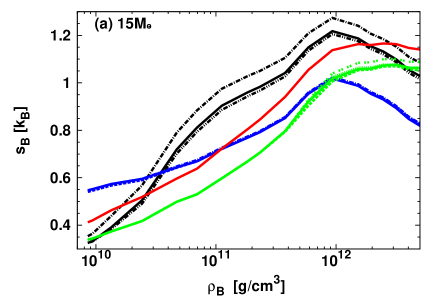
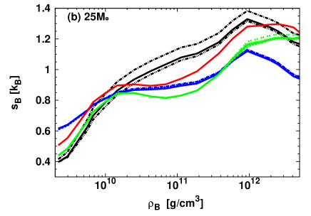
Figure 11: Baryonic entropies per baryon at the centers of the collapsing cores of supernova progenitors of 15M_⊙ (left panel) and 25M_⊙ (right panel) for models 1B (black dashed-dotted lines), 1D (black double-dotted dashed lines), 1E (black solid lines), 2FB (blue dashed-dotted lines), 2FE (blue solid lines), 2KE (blue dashed lines), 3FE (green solid lines), 3KE (green dashed lines), 3HE (green dotted lines), 3WE (green double-dotted lines), and 4FE (red solid lines).

The central densities and temperatures of the collapsing cores increase adiabatically, and the entropy is an essential quantity for determining the dynamics of core collapse. I therefore compare the baryonic entropies per baryon in Fig. 11. These are given by $s_{B}=-\partial f/\partial T|_{n_{B},Y_{p}}/n_{B}$ and are essentially determined by the kinetic terms of the nuclear components and the temperature derivatives of the internal degrees of freedom, $\partial g_{AZ}(T)/\partial T$, and of the internal free energy, $\partial F_{AZ}(T)/\partial T$. Note from the figure that the entropies differ among the models based on different finite-temperature modeling, even in the initial stages of core collapse. For the models with smaller $X_{h}$, such as for models 1B, 1D, and 1E, the entropy is more likely to be high because of the increase in the population of dripped neutrons. Models 2FB, 2FE, and 2FK at at $\rho_{B}\approx 10^{10}{\rm g/cm}^{3}$ and model 4FE at $\rho_{B}\approx 10^{12}{\rm g/cm}^{3}$ tend to yield high entropies because of the large values of $\partial g^{*}_{AZ}(T)/\partial T$ and $\partial g_{AZ}(T)/\partial T$. These differences in entropy would be influential for the fate of core-collapse supernovae Suwa and Müller (2016); Furusawa et al. (2017c); Nagakura et al. (2018b).

IV Summary and Discussion

I have compared the 14 statistical EOSs for the core collapse of a massive star by systematically changing the bulk properties of nuclear matter, the masses of neutron-rich nuclei, and the treatment of finite-temperature effects in the nuclear model. Overall, the temperature dependencies of the internal degrees of freedom and of the internal free energy are paramount to determining the entropy and nuclear composition during the core-collapse phase. Differences in these quantities among EOSs would affect thermodynamic conditions and ensemble-averaged weak-interaction rates of nuclear electron-captures and neutrino-nucleus coherent scattering Furusawa et al. (2017a); therefore, the dynamics of the core collapse would be sensitive to the treatment of the finite-temperature effects. The parameters of bulk nuclear matter and the theoretical mass data for neutron-rich nuclei do not greatly influence the average mass number or the total mass fraction of heavy nuclei.

Semi-empirical expression for internal degrees of freedom that ignore the temperature dependence of shell effects may not be appropriate for discussions of core-collapse nuclei, because they overestimate the number densities of magic nuclei. More precise calculations for internal partition functions are required. The individual level densities of medium-mass, neutron-rich nuclei however, have not been well studied. Actually, some important nuclei lack the data Rauscher (2003) used in the present work. Phenomenological models with nuclear shell washout tend to increase the populations of nuclei with small mass numbers that have large electron-capture rates; they would therefore reduce the charge fraction and entropy significantly in collapse simulations Furusawa et al. (2017a); Nagakura et al. (2018b). The washout formulation for the nuclear shell energies, however, is very simple and some parts, especially its mass-number dependence, should be improved.

Some studies based on EOSs with semi-empirical expression for internal degrees of freedom Sullivan et al. (2016); Titus et al. (2018) indicate that nuclei above the double-magic nuclei, $(N,Z)=(50,28)$ in the nuclear chart are primary targets for studies of electron-capture during core-collapse. In all the EOSs discussed in this works, such nuclei as $(N,Z)=(50,30)$ are certainly populated, while non-magic nuclei are also abundant in the EOSs with more-reliable finite-temperature modeling. Non-magic nuclei, such as $(N,Z)=(40,25)$ and $(60,35)$, may also contribute to the deleptonization of the core Furusawa et al. (2017a). I conclude that further investigations of the internal partition functions of nuclei with proton numbers 25–45 and the neutron numbers 40–85 at $T\approx$0.5–3.0 MeV are needed to remove one of the serious ambiguities in the input physics for core-collapse supernova studies. Finite-temperature effects may also change the electron-capture rates themselves in addition to the nuclear abundances Langanke et al. (2003); Dzhioev et al. (2010); Furusawa et al. (2017a); Titus et al. (2018).

It is surprising that the choice of finite-temperature modeling produces significant differences in the entropy and nuclear composition, even at the beginning of core collapse. To perform supernova simulations consistent with stellar evolution calculations, the same internal partition functions should be utilized in both stages. Even in the postprocessing nucleosynthesis calculations for the ejecta of supernova explosions, the thermodynamic conditions at low temperatures and densities should be shared with the dynamical simulations. The setup of mass data and internal degrees of freedom also needs to be better unified for the stages immediately following supernova explosions.

Note that this comparative study is incomplete to cover all nuclear uncertainties. For instance, the bulk free energy of uniform nuclear matter depends not only on bulk properties at nuclear saturations but also on the theoretical approach such as relativistic mean-field theory, variational method, or chiral effective theory Holt and Kaiser (2017). In addition, there are many other works for the nuclear physics inputs, such as a comprehensive study of nuclear level densities based on two backshifted Fermi gas models and a constant-temperature model Egidy and Bucurescu (2005). Very recently, Raduta and Gullemineli Raduta and Gulminelli (2018) have constructed EOS data for supernova simulations based on Gullemineli and Raduta Gulminelli and Raduta (2015) with the level-density data. Further comparison of the EOSs with a focus on the level densities would be interesting.

In this work, I have systematically compared several ingredients as independent inputs for EOS models. In real, the mass data, partition functions, and nuclear matter calculations should be related to each other. For instance, Rauscher’s partition function is calculated by using the nucleon separation energies in the old version of the FRDM mass data, and the WS4 mass data is based on a nuclear model with individual bulk properties, such as $S_{0}$=30.16 MeV. Level-density data consistent with HFB mass data are also provided, which are based on Hartree-Fock-Bogoliubov theory Goriely et al. (2008). Ideally, comparisons of self-consistent EOSs based on a specific nuclear model should be performed. At present, however, first-principles calculations of heavy nuclei have not been completed, even for ground-state nuclei. More realistic supernova simulations, and predictions that can be compared with neutrino and gravitational wave observations, will require step-by-step improvements in the calculations of nuclear matter, nuclear masses, internal degrees of freedom and weak-interaction rates as nuclear physics inputs.

Model	finite-temperature modeling	mass data	bulk parameter	$\sigma_{0}$ [MeV/fm2]	$C_{s}$
1B	SMSM	–	B	–	–
1D	SMSM	–	D	–	–
1E	SMSM	–	E	–	–
2FB	LDM + washout	FRDM	B	1.047	19.66
2FD	LDM + washout	FRDM	D	1.052	29.68
2FE	LDM + washout	FRDM	E	1.042	28.36
2HE	LDM + washout	HFB24	E	1.042	27.12
2KE	LDM + washout	KTUY	E	1.042	32.16
2WE	LDM + washout	WS4	E	1.042	28.91
3FE	Fai $\&$ Randrup	FRDM	E	–	–
3HE	Fai $\&$ Randrup	HFB24	E	–	–
3KE	Fai $\&$ Randrup	KTUY	E	–	–
3WE	Fai $\&$ Randrup	WS4	E	–	–
4FE	Rauscher	FRDM	E	–	–

Table 1: List of models used for systematic comparisons. The first four columns provide the model name, the treatment of finite-temperature effects (the SMSM EOS Botvina and Mishustin (2010), a LDM with shell-washout Furusawa et al. (2017b), a semi-empirical formula by Fai and Randrup Fái and Randrup (1982), or a Fermi-gas approach by Rauscher Rauscher (2003)), the theoretical mass data (FRDM Möller et al. (2016), HFB24 Goriely et al. (2013), KTUY Koura et al. (2005), or WS4 Wang et al. (2014)), and the parameter set used for bulk nuclear matter (B, D, or E Oyamatsu and Iida (2003, 2007)). The last two columns provide the values of the surface tension $\sigma_{0}$ for symmetric nuclei and the isospin-dependence parameter $C_{s}$, both for model 2.

parameter set	B	D	E
$n_{0}$ [fm-3]	0.15969	0.16905	0.15979
$\omega_{0}$ [MeV]	-16.184	-16.224	-16.145
$K_{0}$ [MeV]	230	180	230
$S_{0}$ [MeV]	33.550	30.543	31.002
$L$ [MeV]	73.214	30.974	42.498
$-y$ [MeV fm3]	220	350	350

Table 2: Parameters of bulk nuclear matter Oyamatsu and Iida (2003, 2007).