Phase-only Image Based Kernel Estimation for Single Image Blind Deblurring

Abstract

The image motion blurring process is generally modelled as the convolution of a blur kernel with a latent image. Therefore, the estimation of the blur kernel is essentially important for blind image deblurring. Unlike existing approaches which focus on approaching the problem by enforcing various priors on the blur kernel and the latent image, we are aiming at obtaining a high quality blur kernel directly by studying the problem in the frequency domain. We show that the auto-correlation of the absolute phase-only image can provide faithful information about the motion (e.g., the motion direction and magnitude, we call it the  motion pattern in this paper.) that caused the blur, leading to a new and efficient blur kernel estimation approach. The blur kernel is then refined and the sharp image is estimated by solving an optimization problem by enforcing a regularization on the blur kernel and the latent image. We further extend our approach to handle non-uniform blur, which involves spatially varying blur kernels. Our approach is evaluated extensively on synthetic and real data and shows good results compared to the state-of-the-art deblurring approaches.

1 Introduction

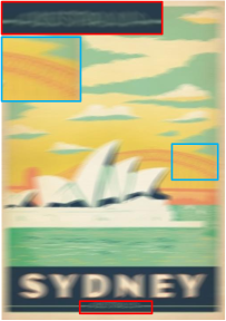
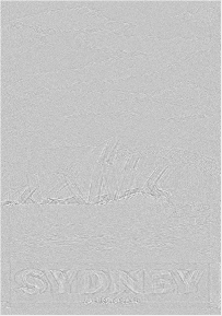
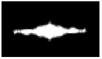
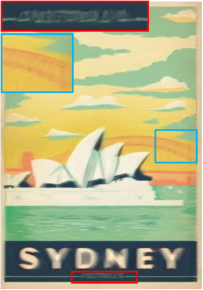
		(c) Auto-correlation
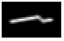
(a) Blurry Image	(b) $P(B)$	(d) Kernel	(e) Nah [19]
(f) Tao [34]	(g) Pan [23]	(h) Yan [43]	(i) Ours

Figure 1: Our deblurring result compared with the state-of-the-art methods. (a) Input blurry image. (b) The phase-only image. (c) The auto-correlation for the phase-only image. (d) The estimated blur kernel. (e) Deblurring result of [19]. (f) Deblurring result of [34]. (g) Deblurring result of [23]. (h) Deblurring result of [43]. (i) Our deblurring result. (Best viewed on screen).

Blind image deblurring aims at estimating the blur kernel and the latent image from an input blurry image. This is an ill-posed problem as there are infinitely many pairs of blur kernels and images that could generate the same blurry image. Blind image deblurring has been extensively studied in computer vision and is still a very active research area [10, 28, 6, 25, 19, 34], where blur kernel estimation is essentially important in obtaining a high quality sharp image.

Existing blind image deblurring methods tend to formulate the problem within the Maximum A Posteriori (MAP) framework, where the blur kernel and the latent sharp image are optimized jointly. To resolve the ill-posed underlining optimization problem, various assumptions, or regularizations, have been proposed for the blur kernel and the desired latent image, such as the dark channel prior [23], extreme channel prior [43], $l_{0}$ regularized prior [22, 41], learned image prior using a CNN [18], uniform blur [17, 42], non-uniform blur from multiple homographies [8, 21], constant depth [7, 39], in-plane rotation [32], and forward motion [45]. The resultant optimization problem is non-convex in general. The blur kernel and the latent image are usually solved in an alternating fashion. Thus, a proper and effective initialization is demanded to achieve a good local optimum solution and makes the algorithm converge quickly.

In this paper, we aim at estimating a high-quality blur kernel directly from the input image with motion blur by studying the problem in the frequency domain. We exploit the phase-only image of the input blurry image, which is reconstructed from the Fourier transformed image using the phase information only. The phase-only image contains edge and texture information about the image structure [20, 27]. The motion (either camera or object motion) information is encoded as repeated image edges in the phase-only image (see Fig. 1 for an example). We show that the auto-correlation of the absolute phase-only image reveals the motion information including the motion direction and motion magnitude, which is referred to as the motion pattern in this paper. It provides information about the blur kernel, thereby leading to a new approach to estimating the blur kernel.

We further improve the blur kernel and latent image estimation by enforcing a spatial sparsity prior on the kernel as well as the latent image gradient in a simple optimization framework. Furthermore, our blur kernel estimation approach can be naturally extended to handle non-uniform blur in order to deal with the spatially-variant blur kernels that arise in complex image deblurring problems. Extensive experiment on both synthetic and real images demonstrate the superiority of our approach over the state-of-the-art methods.

Our main contributions are summarized as follows

1. We propose a new phase-only image-based approach to directly estimating the blur kernel from the input blurry image. The approach for motion pattern estimation is easy and efficient, consisting of a few lines of code.

2. Our single-image blind deblurring model can be naturally extended to handle non-uniform blur in an effective manner. Furthermore, the estimated blur kernel can be easily refined by only enforcing spatial sparsity.

3. Evaluated on both synthetic and real images, our proposed approach shows impressive results compared to other state-of-the-art blind deblurring approaches.

2 Related Work

Single-image blind deblurring. Single-image deblurring jointly estimates the blur kernel and the latent sharp image from the blurry one, which is highly under-constrained since the blurry image could be explained by many pairs of blur kernel and sharp image [11, 24]. In general, image deblurring is formulated in a MAP framework with priors on blur kernels or latent images. The Sparsity prior has proved effective in blur kernel estimation. For instance, Krishnan et al. [15] applied normalized sparsity in their MAP framework to estimate the blur kernel. Xu et al. [42] proposed an approximation of the $l_{0}$-norm as a sparsity prior in order to jointly estimate sharp image and blur kernels. Edge-based methods for blur kernel estimation have been exploited recently [38, 12, 3, 33]. Xu et al. [38] proposed a two-phase method for single-image deblurring. The blur kernel is first estimated based on the selected image edges and refined by ISD optimization. The latent sharp image is then restored by total-variation (TV)-$l_{1}$ deconvolution. In addition, a Gaussian prior is imposed to help the estimation of the blur kernel [12, 3], which leads to an efficient solver. Moreover, the blur kernel has been modelled based on various motion assumptions, such as in-plane camera rotation [32] or camera forward motion [45]. A few works have exploited the layer-wise scene structure to model the blur kernel [7, 8, 21]. Gupta et al. [7] represent the camera motion trajectory using a motion density function, which requires a constant depth or fronto-parallel scene assumption. Hu et al. [8] proposed jointly estimating the depth layering and remove the blur caused by in-plane motion from a single blurry image. Pan et al. [21] proposed jointly estimating object segmentation and camera motion by incorporating soft segmentation. Note that both approaches require user input for initial depth layer segmentation.

Video image blind deblurring. In order to better model non-uniform blur, monocular video and stereo based deblurring approaches are proposed to handle blurring in realistic scenes [26, 39]. Cho et al. [5] proposed a method relying on the assumption that salient sharp frames frequently exist in videos, which only allows for slowly moving objects in dynamic scenes. Wulff and Black [37] proposed a layered model to estimate both foreground motion and background motion. However, these motions are restricted to affine models, and it is difficult to extended them to multi-layer scenes due to the difficulty in depth ordering. Kim and Lee [9] incorporated optical flow estimation to guide the blur kernel estimation, which is able to deal with certain object motion blur. In [10], a new method is proposed to simultaneously estimate optical flow and tackle general blur by minimizing a single non-convex energy function. Stereo images and videos can provide depth information which allows to better model pixel-wise blur kernel. Sellent et al. [28] proposed a stereo video deblurring technique, where 3D scene flow is estimated from the blurry images using a piecewise rigid scene representation. Pan et al. [25] proposed a single framework to jointly estimate the scene flow and deblur the images.

Deep learning based image deblurring. Recently, image deblurring has greatly benefited from the great advances in deep learning [16, 32, 44, 34]. Sun et al. [32] proposed a convolutional neural network (CNN) to estimate locally linear blur kernels. Gong et al. [6] learned optical flow field from a single blurry image directly through a fully-convolutional deep neural network. The blur kernel is then obtained from the estimated optical flow which is applied in an MAP framework to restore the sharp image. Su et al. [31] trained an end-to-end CNN to accumulate information across frames for video deblurring. Nah et al. [19] proposed a multi-scale CNN that restores latent images in an end-to-end learning manner without any assumption on the blur kernel model. Li et al. [18] used a learned image prior to distinguish whether an image is sharp or not and embedded the learned prior into the MAP framework. Tao et al. [34] proposed a light and compact network, SRN-DeblurNet, to deblur the image. While achieving reasonable performance on various scenarios, the success of these deep learning based methods depends on the consistency between the training datasets and the testing datasets, which can hinder the generalization ability.

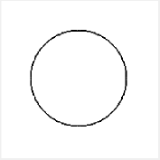
(a) Sharp Image	(b) $|P(\mathbf{L})|$
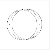
(c) Blurry Image	(d) $|P(\mathbf{B})|$

Figure 2: We use a circle image as an example. The image is blurred by a linear kernel, where the kernel length is 20 pixels and the direction is 10 degree.

3 Method

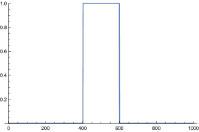
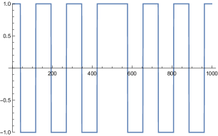
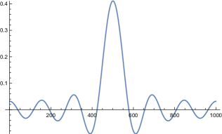
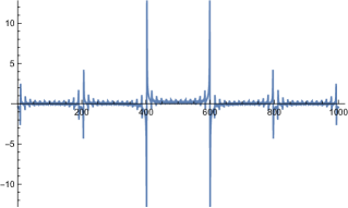
(a) (c) (b) (d)

Figure 3: Given a top-hat function (a), its fourier transform is a $sinc$ shown in (b). (The central peak has twice the width of the others. Note that since the top-hat is symmetric, its Fourier transform is real, hence its phase is either $+1$ or $-1$ shown in (c).) The phase-only image of the top-hat shown in (d) is obtained by taking the inverse Fourier transform of the function in (c).

3.1 Fourier Theory of Phase-only Images

This section contains the main theoretical insights of this paper. Our goal is to find the latent sharp image from a single blurry image. The blurry image can be modelled as a convolution of the latent image with a blur kernel,

$$\mathbf{B}=\mathbf{L}\otimes\mathbf{k},$$ (1)

where $\mathbf{B}$ is the known blurry image, $\mathbf{L}$ denotes the latent sharp image, $\mathbf{k}$ is the blur kernel, $\otimes$ is the convolution operator. Note that this problem is highly under-determined since multiple pairs of $\mathbf{L}$ and $\mathbf{k}$ can lead to the same blurry image.

In the Fourier domain, Eq. (1) corresponds to $\mathcal{F}(\mathbf{B})=\mathcal{F}(\mathbf{L})\odot\mathcal{F}(\mathbf{k})$, where $\odot$ represents the component-wise multiplication.

The phase and amplitude of a complex number $z=ke^{i\theta}$ are $e^{i\theta}$ and $k\geq 0$ respectively. Applying these component-by-component to a Fourier transformed image $\mathcal{F}(\mathbf{L})$ gives the phase and amplitude components. We denote taking the phase of a complex signal by $\mathcal{P}(\cdot)$. Taking the inverse Fourier transform of the phase-component gives the phase-only image, $P(\mathbf{L})=\mathcal{F}^{-1}(\mathcal{P}(\mathcal{F}(\mathbf{L})))$. It is well known that the phase-only image bears more similarity to the original image than the analogously defined amplitude image. Fig. 2 shows an example of the phase-only image derived from a clean and blurry image. As may be observed, taking a phase-only image acts as a sort of edge-extractor. This is related to the fact, noted in [14] that the Fourier components of an edge tend to be in-phase with each other. For a real image $\mathbf{L}$, the phase-only image will also be real. Another simple property is rotation-covariance: if $R$ represents rotation then $P(R(\mathbf{L}))=R(P(\mathbf{L}))$. It is also shift-covariant.

We now make a basic observation regarding the phase-only image of a convolution.

lemma 1.

The phase-only image of a convolution $P(\mathbf{L}\otimes\mathbf{k})$, equals the convolution of the phase-only image and the phase-only kernel.

$$P(\mathbf{L}\otimes\mathbf{k}) =\mathcal{F}^{-1}(\mathcal{P}(\mathcal{F}(\mathbf{L}\otimes\mathbf{k})))=P(\mathbf{L})\otimes P(\mathbf{k})~{}.$$ (2)

This results from a simple calculation.

Linearly-blurred image.

For a simple linear (straight-line) blur kernel, the form of $P(\mathbf{k})$ can be computed. By rotation and shift covariance, it may be assumed without loss of generality, that $\mathbf{k}$ is axis-aligned, in which case $\mathbf{k}(x,y)=\delta(y)H(x)$, where $\delta(y)$ is a Dirac delta function and $H(x)$ is a top-hat. The Fourier transform is separable, so it follows that $P(\mathbf{k})(x,y)=\delta(y)P(H)(x)$. Hence, we investigate what the $1D$ phase-only signal $P(H)$ is. The result is shown in Fig. 3. A formula for the shape of the phase-only top-hat of width $w$ is derived (for the continuous Fourier Transform) in the supplementary material, and is equal to $(\sqrt{2\pi}/w)\,{\rm sinc}(\pi x/w)/\cos(\pi x/w)$, which is plotted in Fig. 3(d). More details of the properties of this function are given in the supplementary material.

According to Eq. (2), if $\mathbf{B}=\mathbf{L}\otimes\mathbf{k}$, then $P(\mathbf{B})$ is obtained by convolving $P(\mathbf{L})$ in the orientation of the linear kernel with the phase-only kernel, shown in Fig. 3(d). This results in the creation of multiple copies (“ghosts”), of the phase-only image, $P(\mathbf{L})$, separated by the width of the filter. (The copies due to the principal peaks will be the most noticeable.) This is shown in Fig. 4.

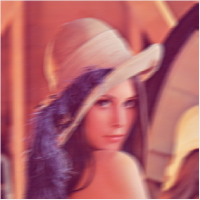
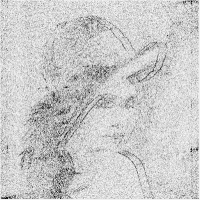
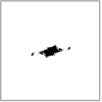
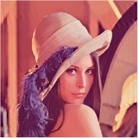
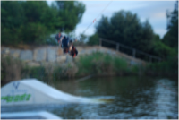
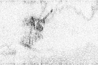
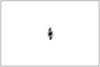
(a) Blurry Image	(b) $|P(\mathbf{B})|$	(c) $\mathcal{A}(|P(\mathbf{B})|)$	(d) Deblurring Results

Figure 4: (a) Input blurry images, the top one is a synthetic image created by ourselves and the bottom one is a real image from dataset [29]. (b) The absolute phase-only image of the blurry image, $|P(\mathbf{B})|$, results in two principal copies (others more faint) of $P(\mathbf{L})$. (c) The autocorrelation of the absolute phase-only image, $\mathcal{A}(|P(\mathbf{B})|)$, showing two distinct peaks (separated by the length of the filter kernel). Distinguishing the two principal peaks of the autocorrelation (apart from the origin) can be used to determine the orientation and width of a linear (straight-line) blur kernel. (d) shows our deblurring results with sharp edges.

The key advantage of phase-only image.

This analysis and the examples show the advantage and purpose in considering the phase-only image as a means of determining the blur kernel, and subsequently deblurring the image. This is illustrated by the analysis of the linear kernel.

The effect of blurring is to smear the image in the blur direction, as shown in Fig. 4 (top left). From this image, it is not easy to discern the shape of the kernel, particularly the linear extent of the kernel. On the other hand, in the phase-only image, the effect of blurring is to create two principal identical copies of $P(\mathbf{L})$ separated by the extent of the blur kernel. This is immediately evident from Fig. 4(b), or Fig. 2(d). Thus, the continuous smear in the blurred image is replaced by a simple sum of two (principle) copies in the phase-only blurred image. This simplification of the effect of blurring makes the further image-processing to compute the blur-kernel much simpler.

This discovery of the application of the phase-only image to deblurring is the key original contribution of this paper, and the supplementary material provides a rigorous mathematical justification of the empirical observation, which we hope the reader will enjoy.

3.2 Autocorrelation

Using phase-only to obtain $P(\mathbf{B})$ from a blurry image results in multiple (two principal) shifted copies of $P(\mathbf{L})$. Note that $P(\mathbf{L})$ is not known. However, this suggests the use of autocorrelation of $P(\mathbf{B})$.

Autocorrelation of a signal $\mathbf{I}$ ($1$ or $2$-dimensional) is computed using Fourier transform as:

$$\mathcal{A}(\mathbf{I})=\mathcal{F}^{-1}(\mathcal{F}(\mathbf{I})\odot\overline{\mathcal{F}(\mathbf{I})}).$$

Unfortunately, if $\mathbf{I}$ is itself a phase-only image, derived from $\mathbf{J}$, then

$$\mathcal{F}(\mathbf{I})=\mathcal{F}(\mathcal{F}^{-1}\mathcal{P}(\mathcal{F}(\mathbf{J})))=\mathcal{P}(\mathcal{F}(\mathbf{J})).$$

So   $\mathcal{A}(\mathbf{I})\!=\!\mathcal{F}^{-1}(\mathcal{P}(\mathcal{F}(\mathbf{J}))\odot\overline{\mathcal{P}(\mathcal{F}(\mathbf{J}))})\!=\!\mathcal{F}^{-1}(1)\!=\delta$
where $\delta$ is a Dirac delta function at the origin. In other words, a phase-only image is completely un-selfcorrelated.

In other words, we cannot derive any information whatever from the autocorrelation of a phase-only image. The solution is to use the absolute value of the phase-only image instead. In other words, we compute $\mathcal{A}(|P(\mathbf{B})|)$, which should show the desired behaviour.

Fig. 4 shows the absolute phase-only image $|P(\mathbf{B})|$ and its autocorrelation $\mathcal{A}(|P(\mathbf{B})|)$. It is noticed that multiple copies of $|P(\mathbf{L})|$ are shown in $|P(\mathbf{B})|$. The most noticeable repeated edges are due to the principal peak of $P(\mathbf{k})$ (as analyzed above) indicating the start and end point of the moving camera.

The autocorrelation of the absolute phase-only image shows several bright points that indicate the motion of the camera, e.g., the motion direction and magnitude, which is referred to as motion pattern. The autocorrelation image will consist of a central peak plus two side-peaks separated by the extent (and in the direction) of the blur-kernel.

Consequently, the motion of the camera will provide faithful information for obtaining the blur kernel. Therefore, in the following section, we will present our approach to image deblurring based on the analysis of the autocorrelation of the absolute phase-only image.

4 Uniform Deblurring

Based on the analysis of the Fourier theory of phase-only images, we introduce our approach to estimate the blur kernel and deblur the images.

4.1 Uniform Blur from Linear Motion

Consider the blur caused by a pure linear motion. By computing the autocorrelation of the absolute phase-only image, the motion pattern, namely the motion direction and the motion magnitude, is extracted by directly connecting the two end bright points in $\mathcal{A}(|P(\mathbf{B})|)$. The blur kernel is then formed based on the extracted motion pattern. In particular, the motion magnitude determines the kernel size. The non-zero kernel values are uniformly distributed along the motion direction (see Fig. 4 the top row for an example). Given the built blur kernel, the latent image can be easily obtained by solving the Eq. (3) which will be introduced in the following section.

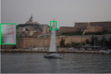
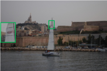
(a) Blurry Image	(b) Nah [19]
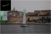
(c) Coarse Kernel	(d) Refined Kernel

Figure 5: (a) The blurry image from dataset [23]. (b) Deblurring results of [19]. (c) Our deblurring result with the coarse blur kernel built from the autocorrelation of the absolute phase-only image. (d) Our deblurring result with the refined kernel. The refined kernel can better improve the deblurring result by looking at the close-up of the part of the sail with detailed sharp edges. Note that the blur kernel is zoomed in the corner.

4.2 Uniform Blur from Non-linear Motion

The blurry image is formed by the integral of light intensity over the exposure period. For more complex motion, the autocorrelation image $\mathcal{A}(|P(\mathbf{B})|)$ will show more bright points representing high correlation values (see Fig. 1 (c) and Fig. 4 (c) for examples).

In general, in the case of uniform (spatially-invariant) blur, one may write $\mathbf{B}=\mathbf{k}\otimes\mathbf{L}$, so, allowing for the possibility of noise, the deblurring problem (with known kernel) may be formulated as finding ${\rm argmin}_{\mathbf{L}}\left\|\mathbf{k}\otimes\mathbf{L}-\mathbf{B}\right\|_{2}^{2}$. In most cases, however, blurring acts as a form of low-pass filter – high-frequency information is lost. Consequently, this problem is not well-conditioned. Thinking of convolution with known $\mathbf{k}$ as being a linear operator, there exist near-zero eigenvalues whose eigenvectors correspond to high-frequency components of the signal (image). The deblurring process is to restore the lost frequency components of the image. If high-frequency components are over-emphasized in the deblurring process, the resulting latent image $\mathbf{L}$ will be noisy, or edges will show ringing. A common solution to this is to add a regularization term that discourages excessive high-frequency components. One is therefore led to the following minimization problem.

$$\min_{\mathbf{L}}\left\|{\mathbf{k}}\otimes\mathbf{L}-\mathbf{B}\right\|_{2}^{2}+\mu_{2}\,h(\nabla\mathbf{L})~{},$$ (3)

where $h(\cdot)$ is a penalty term used to discourage excessive gradients, which are indicative of noise and over-emphasized edges.

In the case of non-linear motion, the kernel is not known exactly, but an initial value of $\mathbf{k}$ may be estimated directly from the autocorrelation of the absolute phase-only image as described previously. Our final goal is to further refine the kernel $\mathbf{k}$ and estimate the latent sharp image $\mathbf{L}$ by solving

$$\min_{\mathbf{L},\mathbf{k}}\left\|\mathbf{k}\otimes\mathbf{L}-\mathbf{B}\right\|_{2}^{2}+\mu_{1}\left\|\mathbf{k}\right\|_{\mathrm{2}}^{2}+\mu_{2}\,h(\nabla\mathbf{L})~{},$$ (4)

where $\mu_{1}$ and $\mu_{2}$ are weight parameters. The first term encodes the fact that the modelled blurry image should be similar to the observed image. The second term is to regularize the solution of the blur kernel. The third term prevents over-sharpening.

The optimization of our energy function defined in Eq. (4) involves two sets of variables, the kernel and the latent image. We perform the minimization iteratively starting with the initial estimate of $\mathbf{k}$ given by the phase-only technique. (See Fig. 5 for an example).

4.2.1 Estimating the Latent Image

The goal is to minimize Eq. (4) by alternation. If $\mathbf{k}$ is known, the problem comes down to minimizing Eq. (3).

Specifically, we use a truncated-quadratic gradient regularization term

$$h(\nabla\mathbf{L})=\sum_{x,y}\,\min\big{(}\left\|\nabla_{xy}\mathbf{L}/\epsilon\right\|^{2},1\big{)}$$

where $\epsilon\in[0.1,1]$ and $\nabla_{xy}\mathbf{L}$ represents the gradient of $\mathbf{L}$ at image coordinates $(x,y)$. This regularization term smooths out small noise, while allowing occasional large gradients (intensity differences). This type of term, proposed by [2] is widely used to regularize noise and gradients in stereo [35] and was also used in deblurring in [42]). Because the truncated quadratic is non-convex, the optimization problem is non-convex. We use the method of half quadratic splitting, as in  [40], to minimize this cost function, though other methods such as Iterative Reweighted Least Squares could be used for such truncated-quadratic cost [1].

4.2.2 Refining the Kernel

Now, with ${\mathbf{L}}$ known, the motion blur kernel can be refined by solving

$$\min_{\mathbf{k}}\left\|\mathbf{k}\otimes{\mathbf{L}}-\mathbf{B}\right\|_{2}^{2}+\mu_{1}\left\|\mathbf{k}\right\|_{\mathrm{2}}^{2}~{}.$$

This is a quadratic problem, and can be solved directly by taking gradients, which results in a set of linear equations. More efficiently, we solve it in the Fourier domain, in which case there is a closed-form solution

$$\mathcal{F}(\mathbf{k})=\overline{\mathcal{F}(\mathbf{L})}\odot\mathcal{F}(\mathbf{B})~{}\big{/}~{}\big{(}\overline{\mathcal{F}(\mathbf{L})}\odot\mathcal{F}(\mathbf{L})+\mu_{1}\big{)}~{},$$

where the division is carried out point-wise (as are the multiplications). Then $\mathbf{k}$ is found by the inverse transform, and then normalized to sum to $1$.

The algorithm alternates between recomputing $\mathbf{L}$ and $\mathbf{k}$ until convergence, or for a fixed number of steps.

5 Extension to Non-uniform Deblurring

(a) Blurry Image	(b) Ours (Uniform)
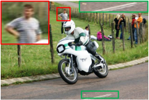
(c) Nah [19]	(d) Gong [6]
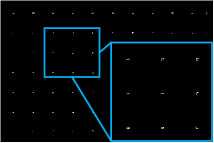
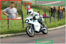
(e) Blur Kernel	(f) Ours (Non-uniform)

Figure 6: Example of our non-uniform blur kernel where the real blurry image is from [6]. (a) Input blurry image. (b) Our deblurring results by using uniform blur model and its blur kernel. We can see clearly that the man in a plaid shirt seems not deblurred because of the improper kernel. (c) Deblurring result of [19]. (d) Deblurring result of [6]. (e) Non-uniform blur kernel. (f) Our deblurring result by using non-uniform blur model and kernel.

Our method can be easily extended to handle non-uniform blur (e.g., the background and foreground undergo different blur) by deblurring the image patch-by-patch or layer-by-layer. Each patch or layer of the image corresponds to a different blur kernel. The new non-uniform blur model can be expressed as

$$\mathbf{B}=\sum_{i=1}^{N}{\mathbf{k}}_{i}\otimes{\mathbf{l}}_{i},$$ (5)

where $N$ denotes the number of segmented patches or layers, $\mathbf{l}_{i}={\bf M}_{i}\odot\mathbf{L}$ is to extract the $i$-th patch or layer of the latent image, ${\bf M}_{i}$ is a binary mask with non-zeros values in the region corresponding to the $i$-th patch or layer in $\mathbf{L}$, and $\mathbf{k}_{i}$ denotes the blur kernel corresponding to the $i$-th patch. Similary, we define $\mathbf{B}_{i}=\mathbf{k}_{i}\otimes\mathbf{l}_{i}$ and $\mathbf{B}=\sum_{i=1}^{N}\mathbf{B}_{i}$. Each layer can be handled using our proposed uniform deblurring approach in Section 4. The final latent image $\mathbf{L}$ is $\sum_{i=1}^{N}{\mathbf{l}_{i}}$. In Fig. 6, we give an example of the deblurring results for uniform and non-uniform blur models. The image is a real blurry image from dataset [6]. Clearly, our non-uniform deblurring achieves better results than our uniform-deblurring model and the other existing non-uniform deblurring methods which either use additional depth, camera pose information [8, 7, 36] or use deep convolutional neural networks [6, 19].

6 Experiment

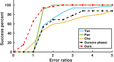
Figure 7: Quantitative evaluations on dataset [17]. We report the experimental results with and without using the blur kernel estimated from the phase-only image (’Ours(no phase)’). The results further demonstrate the effectiveness of blur kernel estimation from the phase-only image.

Table 1: Quantitave comparison on the dataset [17].

	Cho [4]	Pan [23]	Yan [43]	Our (no phase)	Our
PSNR(dB)	25.63	27.54	24.70	25.74	28.38
SSIM	0.7907	0.8626	0.8760	0.7842	0.9250
SSD	2.6688	1.2747	1.6802	3.2517	0.8776

6.1 Experimental Setup

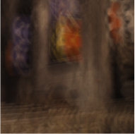
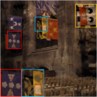
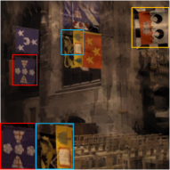
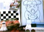
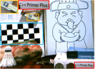
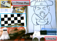
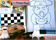
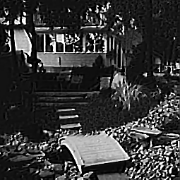
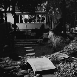
(a) Blurry Image	(b) Yan [43]	(c) Pan [23]	(d) Ours

Figure 8: Qualitative comparison on example images from dataset [13](top), [17](bottom) and image taken by ourselves (middle). (a) Input blurry images. (b) Deblurring results of [43]. (c) Deblurring results of [23]. (d) Our deblurring result. (Best viewed on screen).

Table 2: Quantitative comparisons on the dataset [13], where [19, 16] are deep based methods.

	Blurry Image	Whyte et al. [36]	Xu et al. [42]	Pan et al. [23]	Yan et al. [43]	Nah et al. [19]	Kupyn et al. [16]	Ours
PSNR(dB)	24.93	27.03	27.47	29.95	28.42	26.48	26.10	30.18
SSIM	0.783	0.809	0.811	0.932	0.897	0.807	0.816	0.933

Dataset. We evaluate our approach on the datasets provided by [13, 23, 30, 6, 17] and images captured by ourselves, which covers images from man-made scene, natural scene and images containing text (see Fig. 5, 6, 8 for examples).

Baselines and evaluation metric. Since our proposed approach can handle both uniform and non-uniform blurs, we compare with state-of-the-art methods for both cases separately. For traditional methods (non-deep learning methods), we compare with  [43, 23, 3, 36, 42]. For deep learning based methods, we compare with [6, 19, 16] which can handle spatially-variant blur. We report the PSNR, SSIM on datasets [17, 13] and error ratio on dataset [17] which provides the ground truth blur kernels for evaluation.

Implementation details. We validate the parameters in our model on three reserved images for each dataset and use coarse-to-fine strategy for deblurring. We set $\mu_{1}=2$, $\mu_{2}=0.005$ for our experiment. Our framework is implemented using MATLAB with C++ wrappers. It takes around 40 second to process one image ($800\times 800$) on a single i7 core running at 3.6 GHz.

6.2 Experimental Results

The dataset introduced in [17] is a widely used uniform blur dataset, which contains 32 blurry images generated by 4 ground truth images and 8 blur kernels. We perform the quantitative and qualitative evaluation on this dataset. Results are shown in Fig. 7, 8 and Table 1, which demonstrates that our proposed approach achieves competitive results.

The Natural dataset is generated by [13] with camera motion measured and controlled by a Vicon tracking system. Specifically, the dataset provides blurry image, its latent image, and ground truth blur kernel, which allows the quantitative comparison of our approach with baselines. The captured images are of size $800\times 800$. In Table 2, we show the quantitative comparison with the state-of-the-art Single-image deblurring approaches on dataset [13]. It demonstrates that our approach can achieve the best performance on the PSNR and SSIM score.

We further show the corresponding qualitative comparison results on example images in [13] in Fig. 8. It clearly shows that our approach can recover more sharp details and with less ringing artifacts than other approaches, which are highlighted in the presented results. We also report our deblurring result in Fig. 1, 4, 5 and 6, respectively. Note that our deblurring results can recover the color more faithfully than the baselines.

7 Conclusions

Our proposed phase-only image based kernel estimation approach is simple (implemented in a few lines of code). The resulted image deblurring algorithm achieves better quantitative results (using PSNR, SSIM, and SSD), than the state-of-the-art methods by extensive evaluation on the benchmark datasets. While our approach can handle the general blur cases, it still suffers from low lighting condition like other deblurring methods. Our future work will explore how to remove blurs less sensitive to lighting conditions.

References

- [1] Khurrum Aftab and Richard Hartley. Convergence of iteratively re-weighted least squares to robust m-estimators. In Applications of Computer Vision (WACV), 2015 IEEE Winter Conference on, pages 480–487. IEEE, 2015.
- [2] Andrew Blake and Andrew Zisserman. Visual Reconstruction. MIT Press, Cambridge, MA, USA, 1987.
- [3] Sunghyun Cho and Seungyong Lee. Fast motion deblurring. ACM Trans. Graph., 28:145:1–145:8, 2009.
- [4] Sunghyun Cho, Jue Wang, and Seungyong Lee. Handling outliers in non-blind image deconvolution. In Proc. IEEE Int. Conf. Comp. Vis., pages 495–502. IEEE, 2011.
- [5] Sunghyun Cho, Jue Wang, and Seungyong Lee. Video deblurring for hand-held cameras using patch-based synthesis. ACM Transactions on Graphics (TOG), 31(4):64, 2012.
- [6] Dong Gong, Jie Yang, Lingqiao Liu, Yanning Zhang, Ian Reid, Chunhua Shen, Anton van den Hengel, and Qinfeng Shi. From motion blur to motion flow: A deep learning solution for removing heterogeneous motion blur. In Proc. IEEE Conf. Comp. Vis. Patt. Recogn., pages 2319–2328, 2017.
- [7] Ankit Gupta, Neel Joshi, C Lawrence Zitnick, Michael Cohen, and Brian Curless. Single image deblurring using motion density functions. In Proc. Eur. Conf. Comp. Vis., pages 171–184. Springer, 2010.
- [8] Zhe Hu, Li Xu, and Ming-Hsuan Yang. Joint depth estimation and camera shake removal from single blurry image. In Proc. IEEE Conf. Comp. Vis. Patt. Recogn., pages 2893–2900, 2014.
- [9] Tae Hyun Kim and Kyoung Mu Lee. Segmentation-free dynamic scene deblurring. In Proc. IEEE Conf. Comp. Vis. Patt. Recogn., pages 2766–2773, 2014.
- [10] Tae Hyun Kim and Kyoung Mu Lee. Generalized video deblurring for dynamic scenes. In Proc. IEEE Conf. Comp. Vis. Patt. Recogn., pages 5426–5434, 2015.
- [11] Hui Ji and Chaoqiang Liu. Motion blur identification from image gradients. In 2008 IEEE Conference on Computer Vision and Pattern Recognition, pages 1–8. IEEE, 2008.
- [12] Neel Joshi, Richard Szeliski, and David J Kriegman. Psf estimation using sharp edge prediction. In Proc. IEEE Conf. Comp. Vis. Patt. Recogn., pages 1–8, 2008.
- [13] Rolf Köhler, Michael Hirsch, Betty Mohler, Bernhard Schölkopf, and Stefan Harmeling. Recording and playback of camera shake: Benchmarking blind deconvolution with a real-world database. In Proc. Eur. Conf. Comp. Vis., pages 27–40. Springer, 2012.
- [14] Peter Kovesi. Phase congruency detects corners and edges. In DICTA, 2003.
- [15] Dilip Krishnan, Terence Tay, and Rob Fergus. Blind deconvolution using a normalized sparsity measure. In Proc. IEEE Conf. Comp. Vis. Patt. Recogn., pages 233–240, 2011.
- [16] Orest Kupyn, Volodymyr Budzan, Mykola Mykhailych, Dmytro Mishkin, and Jiri Matas. Deblurgan: Blind motion deblurring using conditional adversarial networks. ArXiv e-prints, 2017.
- [17] Anat Levin, Yair Weiss, Fredo Durand, and William T Freeman. Understanding and evaluating blind deconvolution algorithms. In Proc. IEEE Conf. Comp. Vis. Patt. Recogn., pages 1964–1971, 2009.
- [18] Lerenhan Li, Jinshan Pan, Wei-Sheng Lai, Changxin Gao, Nong Sang, and Ming-Hsuan Yang. Learning a discriminative prior for blind image deblurring. In Proc. IEEE Conf. Comp. Vis. Patt. Recogn., pages 6616–6625, 2018.
- [19] Seungjun Nah, Tae Hyun Kim, and Kyoung Mu Lee. Deep multi-scale convolutional neural network for dynamic scene deblurring. In Proc. IEEE Conf. Comp. Vis. Patt. Recogn., July 2017.
- [20] A Oppenheim and J. Lim. The importance of phase in signals. Proceedings of the IEEE, 69:529–541, 1981.
- [21] Jinshan Pan, Zhe Hu, Zhixun Su, Hsin-Ying Lee, and Ming-Hsuan Yang. Soft-segmentation guided object motion deblurring. In Proc. IEEE Conf. Comp. Vis. Patt. Recogn., pages 459–468, 2016.
- [22] Jinshan Pan, Zhe Hu, Zhixun Su, and Ming-Hsuan Yang. Deblurring text images via l0-regularized intensity and gradient prior. In Proc. IEEE Conf. Comp. Vis. Patt. Recogn., pages 2901–2908, 2014.
- [23] Jinshan Pan, Deqing Sun, Hanspeter Pfister, and Ming-Hsuan Yang. Blind image deblurring using dark channel prior. In Proc. IEEE Conf. Comp. Vis. Patt. Recogn., pages 1628–1636, 2016.
- [24] Liyuan Pan, Yuchao Dai, and Miaomiao Liu. Single image deblurring and camera motion estimation with depth map. In 2019 IEEE Winter Conference on Applications of Computer Vision (WACV), pages 2116–2125. IEEE, 2019.
- [25] Liyuan Pan, Yuchao Dai, Miaomiao Liu, and Fatih Porikli. Simultaneous stereo video deblurring and scene flow estimation. In Proc. IEEE Conf. Comp. Vis. Patt. Recogn., July 2017.
- [26] Liyuan Pan, Yuchao Dai, Miaomiao Liu, and Fatih Porikli. Depth map completion by jointly exploiting blurry color images and sparse depth maps. In IEEE Winter Conference on Applications of Computer Vision (WACV), pages 1377–1386, 2018.
- [27] Giuseppe Papari and Nicolai Petkov. Edge and line oriented contour detection: State of the art. Image and Vision Computing, 29(2-3):79–103, 2011.
- [28] Anita Sellent, Carsten Rother, and Stefan Roth. Stereo video deblurring. In Proc. Eur. Conf. Comp. Vis., pages 558–575. Springer, 2016.
- [29] Jianping Shi, Li Xu, and Jiaya Jia. Discriminative blur detection features. In Proc. IEEE Conf. Comp. Vis. Patt. Recogn., pages 2965–2972, 2014.
- [30] Jürgen Sturm, Nikolas Engelhard, Felix Endres, Wolfram Burgard, and Daniel Cremers. A benchmark for the evaluation of rgb-d slam systems. In IEEE/RSJ International Conference on Intelligent Robots and Systems, pages 573–580, 2012.
- [31] Shuochen Su, Mauricio Delbracio, Jue Wang, Guillermo Sapiro, Wolfgang Heidrich, and Oliver Wang. Deep video deblurring for hand-held cameras. In Proc. IEEE Conf. Comp. Vis. Patt. Recogn., July 2017.
- [32] Jian Sun, Wenfei Cao, Zongben Xu, and Jean Ponce. Learning a convolutional neural network for non-uniform motion blur removal. In Proc. IEEE Conf. Comp. Vis. Patt. Recogn., pages 769–777, 2015.
- [33] Libin Sun, Sunghyun Cho, Jue Wang, and James Hays. Edge-based blur kernel estimation using patch priors. In Proc. IEEE Int. Conf. Computational Photography, 2013.
- [34] Xin Tao, Hongyun Gao, Xiaoyong Shen, Jue Wang, and Jiaya Jia. Scale-recurrent network for deep image deblurring. In Proc. IEEE Conf. Comp. Vis. Patt. Recogn., June 2018.
- [35] Olga Veksler. Stereo matching by compact windows via minimum ratio cycle. In Proc. IEEE Int. Conf. Comp. Vis., volume 1, pages 540–547. IEEE, 2001.
- [36] Oliver Whyte, Josef Sivic, Andrew Zisserman, and Jean Ponce. Non-uniform deblurring for shaken images. Int. J. Comp. Vis., 98(2):168–186, 2012.
- [37] Jonas Wulff and Michael Julian Black. Modeling blurred video with layers. In Proc. Eur. Conf. Comp. Vis., pages 236–252. Springer, 2014.
- [38] Li Xu and Jiaya Jia. Two-phase kernel estimation for robust motion deblurring. In Proc. Eur. Conf. Comp. Vis., pages 157–170. Springer, 2010.
- [39] Li Xu and Jiaya Jia. Depth-aware motion deblurring. In Proc. IEEE Int. Conf. Computational Photography, pages 1–8, 2012.
- [40] Li Xu, Cewu Lu, Yi Xu, and Jiaya Jia. Image smoothing via l0 gradient minimization. ACM Trans. Graph., 30:174:1–174:12, 2011.
- [41] Li Xu, Xin Tao, and Jiaya Jia. Inverse kernels for fast spatial deconvolution. In Proc. Eur. Conf. Comp. Vis., pages 33–48. Springer, 2014.
- [42] Li Xu, Shicheng Zheng, and Jiaya Jia. Unnatural l0 sparse representation for natural image deblurring. In Proc. IEEE Conf. Comp. Vis. Patt. Recogn., pages 1107–1114, 2013.
- [43] Yanyang Yan, Wenqi Ren, Yuanfang Guo, Rui Wang, and Xiaochun Cao. Image deblurring via extreme channels prior. In Proc. IEEE Conf. Comp. Vis. Patt. Recogn., pages 6978–6986, 2017.
- [44] Jiawei Zhang, Jinshan Pan, Jimmy Ren, Yibing Song, Linchao Bao, Rynson W.H. Lau, and Ming-Hsuan Yang. Dynamic scene deblurring using spatially variant recurrent neural networks. In Proc. IEEE Conf. Comp. Vis. Patt. Recogn., June 2018.
- [45] Shicheng Zheng, Li Xu, and Jiaya Jia. Forward motion deblurring. In Proc. IEEE Int. Conf. Comp. Vis., December 2013.