Antiadiabatic phonons, Coulomb pseudopotential and superconductivity in Eliashberg – McMillan theory

Abstract

The influence of antiadiabatic phonons on the temperature of superconducting transition is considered within Eliashberg – McMillan approach in the model of discrete set of (optical) phonon frequencies. A general expression for superconducting transition temperature $T_{c}$ is proposed, which is valid in situation, when one (or several) of such phonons becomes antiadiabatic. We study the contribution of such phonons into the Coulomb pseudopotential $\mu^{\star}$. It is shown, that antiadiabatic phonons do not contribute to Tolmachev’s logarithm and its value is determined by partial contributions from adiabatic phonons only. The results obtained are discussed in the context of the problem of unusually high superconducting transition temperature of FeSe monolayer on STO.

71.20.-b, 71.27.+a, 71.28.+d, 74.70.-b

1 Introduction

The most developed approach to description of superconductivity in the system of electrons and phonons is Eliashberg – McMillan theory [1, 2, 3, 4]. It is well known, that this theory is completely based on the applicability of adiabatic approximation and Migdal theorem [5], which allows to neglect vertex corrections in calculations of the effects of electron – phonon interaction in typical metals. The real small parameter of perturbation theory is $\lambda\frac{\Omega_{0}}{E_{F}}\ll 1$, where $\lambda$ is the dimensionless coupling constant of electron – phonon interaction, $\Omega_{0}$ is characteristic phonon frequency and $E_{F}$ is Fermi energy of the electrons. In particular, this leads to a conclusion, that vertex corrections in this theory can be neglected even for $\lambda>1$, because of the validity of inequality $\frac{\Omega_{0}}{E_{F}}\ll 1$ characteristic for typical metals.

In a recent paper [6] we have shown, that under the conditions of strong nonadiabaticity , when $\Omega_{0}\gg E_{F}$, a new small parameter appears in the theory $\lambda_{D}\sim\lambda\frac{E_{F}}{\Omega_{0}}\sim\lambda\frac{D}{\Omega_{0}}\ll 1$ ($D$ is the halfwidth of electron band), so that corrections to electronic spectrum become irrelevant and vertex correction can be similarly neglected [7]. In general case, the renormalization of electronic spectrum (effective mass of an electron) is determined by the new dimensionless constant $\tilde{\lambda}$, which reduces to the usual $\lambda$ in adiabatic limit, while in the strong antiadiabatic limit it tends to $\lambda_{D}$. At the same time, the temperature of superconducting transition $T_{c}$ in antiadiabatic limit is determined by Eliashberg – McMillan pairing coupling constant $\lambda$, while the preexponential factor in the expression for $T_{c}$, which is of the typical weak – coupling form, is determined by band halfwidth (Fermi energy). For the case of the interaction with a single optical phonon in Ref. [6] we obtained the unified expression for $T_{c}$, valid both in adiabatic and antiadiabatic regimes, and producing a smooth interpolation in the intermediate region.

In Ref. [6] we also noted, that the presence of high phonon frequencies of the order of or even exceeding the Fermi energy, leads to the obvious suppression of Tolmachev’s logarithm in the expression for Coulomb pseudopotential $\mu^{\star}$, which creates additional difficulties for the realization of superconducting state in the system with antiadiabatic phonons.

The interest to this problem is stimulated by the discovery of a number superconductors, where adiabatic approximation is not valid, while characteristic phonon frequencies are of the order of or even higher than Fermi energy of electrons. Most typical in this sense are intercalated systems with monolayers of FeSe, as well as monolayers of FeSe on Sr(Ba)TiO₃ (and similar) substrates (FeSe/STO) [8]. For the first time, the nonadiabatic character of superconductivity in FeSe/STO was noted by Gor’kov [9, 10], while discussing the idea of possible mechanism of the enhancement of superconducting transition temperature $T_{c}$ in FeSe/STO system due to interaction with high energy optical phonons of SrTiO₃ [8].

In the present paper we consider the generalized model with discrete set of the frequencies of (optical) phonons, part of which may be andiabatic. We obtain the general expressions for $T_{c}$, valid both in adiabatic and antiadiabatic limits. We also present the general analysis of the problem of the Coulomb pseudopotential in such model. The results obtained are used for simple estimates of $T_{c}$ in situation typical for FeSe/STO.

2 Temperature of superconducting transition

Linearized Eliashberg equations, determining superconducting transition temperature $T_{c}$, written in real frequencies representation, have the following form [2]:

$$[1-Z(\varepsilon)]\varepsilon=\int_{0}^{D}d\varepsilon^{\prime}\int_{0}^{\infty}d\omega\alpha^{2}(\omega)F(\omega)f(-\varepsilon^{\prime})\times$$

$$\times\left(\frac{1}{\varepsilon^{\prime}+\varepsilon+\omega+i\delta}-\frac{1}{\varepsilon^{\prime}-\varepsilon+\omega-i\delta}\right)$$ (1)

$$Z(\varepsilon)\Delta(\varepsilon)=\int_{0}^{D}\frac{d\varepsilon^{\prime}}{\varepsilon^{\prime}}th\frac{\varepsilon^{\prime}}{2T_{c}}Re\Delta(\varepsilon^{\prime})\times$$

$$\times\int_{0}^{\infty}d\omega\alpha^{2}(\omega)F(\omega)\times$$

$$\times\left(\frac{1}{\varepsilon^{\prime}+\varepsilon+\omega+i\delta}+\frac{1}{\varepsilon^{\prime}-\varepsilon+\omega-i\delta}\right)$$ (2)

Here $\Delta(\omega)$ is the gap function of a superconductor, while $Z(\omega)$ is electron mass renormalization function and $f(\varepsilon)$ is Fermi distribution. In difference with the standard approach [2], we have introduced the finite integration limits, determined by the (half)bandwidth $D$. In the following we assume the half–filled band of degenerate electrons in two dimensions, so that $D=E_{F}\gg T_{c}$, with constant density of states. For simplicity at first we neglect the contribution of direct Coulomb repulsion. In these (integral) equations $\alpha^{2}(\omega)$ represents Eliashberg – McMillan function, determining the strength electron – phonon interaction, and $F(\omega)$ is the phonon density of states. Eliashberg – McMillan coupling constant is defined as:

$$\lambda=2\int_{0}^{\infty}\frac{d\omega}{\omega}\alpha^{2}(\omega)F(\omega)$$ (3)

The details concerning its calculation for systems with nonadiabatic phonons were discussed in details in Ref. [6].

Situation is considerably simplified [6], if we consider these equations in the limit of $\varepsilon\to 0$ and look for the solutions $Z(0)=Z$ and $\Delta(0)=\Delta$. Then from (1) we obtain:

$$[1-Z]\varepsilon=-2\varepsilon\int_{0}^{\infty}d\omega\alpha^{2}(\omega)F(\omega)\frac{D}{\omega(\omega+D)}$$ (4)

or

$$Z=1+\tilde{\lambda}$$ (5)

where constant $\tilde{\lambda}$ is defined as:

$$\tilde{\lambda}=2\int_{0}^{\infty}\frac{d\omega}{\omega}\alpha^{2}(\omega)F(\omega)\frac{D}{\omega+D}$$ (6)

which for $D\to\infty$ reduces to the usual Eliasberg – McMillan constant (3), while for $D$ significantly smaller than characteristic phonon frequencies it gives the “antiadiabatic” coupling constant:

$$\lambda_{D}=2D\int\frac{d\omega}{\omega^{2}}\alpha^{2}(\omega)F(\omega)$$ (7)

Eq. (6) describes smooth transition between the limits of wide and narrow conduction bands. Mass renormalization is, in general case, determined exclusively by constant $\tilde{\lambda}$:

$$m^{\star}=m(1+\tilde{\lambda})$$ (8)

In the limit of strong nonadiabaticity this renormalization is quite small and determined by the limiting expression $\lambda_{D}$ [6].

From Eq. (2) in the limit of $\varepsilon\to 0$ and using (5), we immediately obtain the following expression for $T_{c}$:

$$1+\tilde{\lambda}=2\int_{0}^{\infty}d\omega\alpha^{2}(\omega)F(\omega)\int_{0}^{D}\frac{d\varepsilon^{\prime}}{\varepsilon^{\prime}(\varepsilon^{\prime}+\omega)}th\frac{\varepsilon^{\prime}}{2T_{c}}$$ (9)

Consider now the situation with discrete set of phonon modes (dispesionless, Einstein phonons). In this case the phonon density of states is written as:

$$F(\omega)=\sum_{i}\delta(\omega-\omega_{i})$$ (10)

where $\omega_{i}$ are discrete frequencies modeling the optical branches of the phonon spectrum. Then from Eqs. (3) and (6) we have:

$$\lambda=2\sum_{i}\frac{\alpha^{2}(\omega_{i})}{\omega_{i}}\equiv\sum_{i}\lambda_{i}$$ (11)

$$\tilde{\lambda}=2\sum_{i}\frac{\alpha^{2}(\omega_{i})D}{\omega_{i}(\omega_{i}+D)}=2\sum_{i}\lambda_{i}\frac{D}{\omega_{i}+D}\equiv\sum_{i}\tilde{\lambda}_{i}$$ (12)

Correspondingly, in this case:

$$\alpha^{2}(\omega)F(\omega)=\sum_{i}\alpha^{2}(\omega_{i})\delta(\omega-\omega_{i})=\sum_{i}\frac{\lambda_{i}}{2}\omega_{i}\delta(\omega-\omega_{i})$$ (13)

The standard Eliashberg equation (in adiabatic limit) for such model were consistently solved in Ref. [11]. For our purposes it is sufficient to analyze only the Eq. (9), which takes now the following form:

$$1+\tilde{\lambda}=2\sum_{i}\alpha^{2}(\omega_{i})\int_{0}^{D}\frac{d\varepsilon^{\prime}}{\varepsilon^{\prime}(\varepsilon^{\prime}+\omega_{i})}th\frac{\varepsilon^{\prime}}{2T_{c}}$$ (14)

Solving Eq. (14) we obtain:

$$T_{c}\sim\prod_{i}\left(\frac{D}{1+\frac{D}{\omega_{i}}}\right)^{\frac{\lambda_{i}}{\lambda}}\exp\left(-\frac{1+\tilde{\lambda}}{\lambda}\right)$$ (15)

For the case of two optical phonons with frequencies $\omega_{1}$ and $\omega_{2}$ we have:

$$T_{c}\sim\left(\frac{D}{1+\frac{D}{\omega_{1}}}\right)^{\frac{\lambda_{1}}{\lambda}}\left(\frac{D}{1+\frac{D}{\omega_{2}}}\right)^{\frac{\lambda_{2}}{\lambda}}\exp\left(-\frac{1+\tilde{\lambda}}{\lambda}\right)$$ (16)

where $\tilde{\lambda}=\tilde{\lambda}_{1}+\tilde{\lambda}_{2}$ and $\lambda=\lambda_{1}+\lambda_{2}$. For the case of $\omega_{1}\ll D$ (adiabatic phonon), and $\omega_{2}\gg D$ (antiadiabatic phonon) Eq. (16) is immediately reduced to:

$$T_{c}\sim(\omega_{1})^{\frac{\lambda_{1}}{\lambda}}(D)^{\frac{\lambda_{2}}{\lambda}}\exp\left(-\frac{1+\tilde{\lambda}}{\lambda}\right)$$ (17)

Here we can see, that in the preexponential factor the frequency of antiadiabatic phonon is replaced by band halfwidth (Fermi energy), which plays a role of cutoff for logarithmic divergence in Cooper channel in antiadiabatic limit [6, 9, 10].

The general result (15) gives the unified expression for $T_{c}$ for the discrete set of optical phonons, valid both in adiabatic and antiadiabatic regimes and interpolating between these limit in intermediate region.

3 Coulomb pseudopotential

Above we had neglected the direct Coulomb repulsion of electrons, which in the standard approach [1, 2, 3] is described by Coulomb pseudopotential $\mu^{\star}$, which is effectively suppressed by large Tolmachev’s logarithm. As was noted in Ref. [6] antiadiabatic phonons suppress Tolmachev’s logarithm, which apparently leads to a sufficient suppression of the temperature of superconducting transition. To clarify this situation let us consider the simplified version of integral equation for the gap (2), writing it as:

$$Z(\varepsilon)\Delta(\varepsilon)=\int_{0}^{D}d\varepsilon^{\prime}K(\varepsilon,\varepsilon^{\prime})\frac{1}{\varepsilon^{\prime}}th\frac{\varepsilon^{\prime}}{2T_{c}}\Delta(\varepsilon^{\prime})$$ (18)

where the integral kernel we write as a combination of two step – functions:

$$K(\varepsilon,\varepsilon^{\prime})=\lambda\theta(\tilde{D}-|\varepsilon|)\theta(\tilde{D}-|\varepsilon^{\prime}|)-\mu\theta(D-|\varepsilon|)\theta(D-|\varepsilon^{\prime}|)$$ (19)

where $\mu$ is the dimensionless (repulsive) Coulomb potential, while the parameter $\tilde{D}$, determining the energy width of attraction region due to phonons is determined by preexponential factor of Eq. (15):

$$\tilde{D}=\prod_{i}\left(\frac{D}{1+\frac{D}{\omega_{i}}}\right)^{\frac{\lambda_{i}}{\lambda}}$$ (20)

Note that we always have $\tilde{D}<D$. Eq. (18) is now rewritten as:

$$Z(\varepsilon)\Delta(\varepsilon)=(\lambda-\mu)\int_{0}^{\tilde{D}}\frac{d\varepsilon^{\prime}}{\varepsilon^{\prime}}th\frac{\varepsilon^{\prime}}{2T_{c}}\Delta(\varepsilon^{\prime})-\mu\int_{\tilde{D}}^{D}\frac{d\varepsilon^{\prime}}{\varepsilon^{\prime}}\Delta(\varepsilon^{\prime})$$ (21)

Writing the mass renormalization due to phonons as:

$$Z(\varepsilon)=\left\{\begin{array}[]{c}1+\tilde{\lambda}\quad\mbox{for}\quad\varepsilon<\tilde{D}\\ 1\quad\mbox{for}\quad\varepsilon>\tilde{D}\end{array}\right.$$ (22)

we look for the solution of Eq. (18) for $\Delta(\varepsilon)$, as usual, also in two – step form [1, 2, 3]:

$$\Delta(\varepsilon)=\left\{\begin{array}[]{c}\Delta_{1}\quad\mbox{for}\quad\varepsilon<\tilde{D}\\ \Delta_{2}\quad\mbox{for}\quad\varepsilon>\tilde{D}\end{array}\right.$$ (23)

Then Eq. (21) transforms into the system of two homogeneous linear equations for constants $\Delta_{1}$ and $\Delta_{2}$:

$$(1+\tilde{\lambda})\Delta_{1}=(\lambda-\mu)\ln\frac{\tilde{D}}{T_{c}}\Delta_{1}-\mu\ln\frac{D}{\tilde{D}}\Delta_{2}$$

$$\Delta_{2}=-\mu\ln\frac{\tilde{D}}{T_{c}}\Delta_{1}-\mu\ln\frac{D}{\tilde{D}}\Delta_{2}$$ (24)

with the condition for nontrivial solution taking the form:

$$1+\tilde{\lambda}=\left(\lambda-\frac{\mu}{1+\mu\ln\frac{D}{\tilde{D}}}\right)\ln\frac{\tilde{D}}{T_{c}}$$ (25)

Correspondingly, for the transition temperature we get:

$$T_{c}=\tilde{D}\exp\left(-\frac{1+\tilde{\lambda}}{\lambda-\mu^{\star}}\right)$$ (26)

where the Coulomb pseudopotential is determined by the following expression:

$$\mu^{\star}=\frac{\mu}{1+\mu\ln\frac{D}{\tilde{D}}}=\frac{\mu}{1+\mu\ln\prod_{i}\left(1+\frac{D}{\omega_{i}}\right)^{\frac{\lambda_{i}}{\lambda}}}$$ (27)

Thus, the phonon frequencies enter Tolmachev’s logarithm as the product of partial contributions, with values determined also by corresponding coupling constants. Similar structure of Tolmachev’s logarithm was first obtained (in somehow different model) in Ref. [12], where the case of frequencies going outside the limits of adiabatic approximation was not considered. In this sense, Eq. (27) has a wider region of applicability. In particular, for the model of two optical phonons with frequencies $\omega_{1}\ll D$ (adiabatic phonon) and $\omega_{2}\gg D$, from Eq. (27) we get:

$$\mu^{\star}=\frac{\mu}{1+\mu\ln\left(\frac{D}{\omega_{1}}\right)^{\frac{\lambda_{1}}{\lambda}}}=\frac{\mu}{1+\mu\frac{\lambda_{1}}{\lambda}\ln\frac{D}{\omega_{1}}}$$ (28)

We can see, that the contribution of antiadiabatic phonon drops out of Tolmachev’s logarithm, while the logarithm itself remains, with its value determined by the ratio of the band halfwidth (Fermi energy) to the frequency of adiabatic (low frequency) phonon. The general effect of suppression of Coulomb repulsion also remains, though it becomes weaker proportionally to to the partial interaction of electrons with corresponding phonon. This situation is conserved also in the general case — the value of Tolmachev’s logarithm and corresponding Coulomb pseudopotential is determined by contributions of adiabatic phonons, while antiadiabatic phonons drops out. Thus, in general case, situation becomes more favorable for superconductivity, as compared to the case of a single antiadiabatic phonon, considered in Ref. [6].

4 Conclusions

In the present paper we have considered the electron – phonon coupling in Eliashberg – McMillan theory in situation, when antiadiabatic phonons with high enough frequency (comparable or exceeding the Fermi energy $E_{F}$) are present in the system. The value of mass renormalization, in general case, is determined by the coupling constant $\tilde{\lambda}$, while the value of the pairing interaction is always determined by the standard coupling constant $\lambda$ of Eliashberg – McMillan theory, appropriately generalized by taking into account the finite value of phonon frequency [6]. Mass renormalization due to antiadiabatic phonons is small and determined by the coupling constant $\lambda_{D}\ll\lambda$. In this sense, in the limit of strong antiadiabaticity, the coupling of such phonons with electrons becomes weak and corresponding vertex correction are irrelevant [7], similarly to the case of adiabatic phonons [5]. Precisely this this fact allows us to use Eliashberg – McMillan approach in the limit of strong antiadiabaticity. In the intermediate region all expressions proposed above are of interpolating nature and for more deep understanding of this region we have to use other approaches (see e.g. Refs. [13, 14]).

The cutoff of pairing interaction in Cooper channel in antiadiabatic limit takes place at energies $\sim E_{F}$, as was previously noted in Refs. [6, 9, 10]), so that corresponding phonons do not contribute to Tolmachev’s logarithm in Coulomb pseudopotential, though large enough values of this logarithm (and corresponding smallness of $\mu^{\star}$) can be guaranteed due to contributions from adiabatic phonons.

Note that above we have used rather simplified analysis of Eliashberg equations. However, in our opinion, more elaborate approach, e.g. along the lines of Ref. [11], will not lead to qualitative change of our results.

In conclusion let us discuss the current results in the context of possible explanation of high – temperature superconductivity in a monolayer of FeSe on Sr(Ba)TiO₃ (FeSe/STO) [8]. The presence in Sr(Ba)TiO₃ of high – energy optical phonons indicates the possibility of significant enhancement of $T_{c}$ in this system due to interactions of FeSe electrons with these phonons on FeSe/STO interface [8, 15]. ARPES experiments [15] and LDA+DMFT calculations [16, 17] have shown, that Fermi energy $E_{F}$ in this system is significantly (practically two times) lower than the energy of the optical phonon, which unambigously indicates the realization, in this case, of antiadiabatic situation [9, 10]. Let us look if we can explain the observed high values of $T_{c}$ in this system using the expressions derived in this work. Assuming for FeSe on STO the characteristic value of phonon frequency $\omega_{1}=$ 350K, Fermi energy $E_{F}=D=$ 650K, and the energy of the optical phonon in SrTiO₃ $\omega_{2}=$ 1000K [8, 15], we calculate $T_{c}$ using Eqs. (16), (26) (the case two phonon frequencies), considering $\mu^{\star}$ as a free model parameter. Let us choose the value of $\lambda_{1}$ to obtain, in the absence of interactions with high – energy phonon of STO, the value of $T_{c}=$ 9K, typical for the bulk FeSe, which gives $\lambda_{1}>$ 0.4. Results of our calculations are shown in Fig. 1. We can see that the experimentally observed [8] high values of $T_{c}\sim$ 60–80K can be obtained only for large enough values of the coupling constant of FeSe electrons with high – energy optical phonon of STO $\lambda_{2}>$ 0.5, so that the total pairing coupling constant $\lambda=\lambda_{1}+\lambda_{2}>$ 0.9. Strictly speaking, such values of the coupling constants can not be considered something unusual. However, the appearance of these large values in FeSe/STO system seems rather improbable in the light of qualitative estimates of $\lambda$ for nonadiabatic case in Ref. [6], as well as the results of ab initio calculations of $\lambda$ for this system [18]. Note also, that the values of the parameters used here for FeSe/STO belong to the intermediate region between adiabatic or nonadiabatic regions, where our expressions, as was stressed above, are of interpolating nature. Variation of the values of these parameters in relatively wide range does not lead to the qualitative change of our results. Traditionally low values of $\mu^{\star}$ used here, can not be obtained for the assumed values of $D=E_{F}$, $\omega_{1}$ and coupling constants from expressions like (28) with usual values of $\mu$, due to rather small values of corresponding Tolmachev’s logarithm.

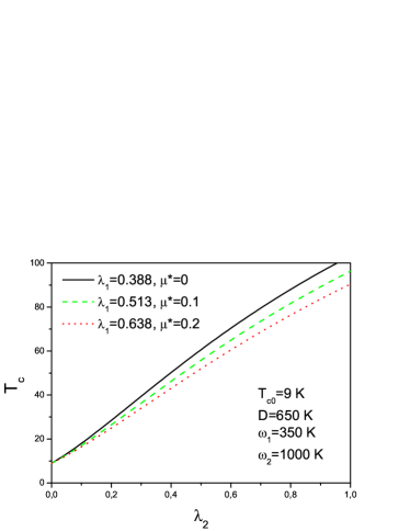
Figure 1: Fig. 1. Dependence of superconducting transition temperature on the coupling constant with high – energy phonon for the typical values of parameters of FeSe/STO system.

The author is grateful to E.Z. Kuchinskii for discussions and help with numerical calculations. This work was partially supported by RFBR grant No. 17-02-00015 and the program of fundamental research No. 12 of the RAS Presidium “Fundamental problems of high – temperature superconductivity”.

References

- [1] D.J. Scalapino. In “Superconductivity”, p. 449, Ed. by R.D. Parks, Marcel Dekker, NY, 1969
- [2] S.V. Vonsovsky, Yu.A. Izyumov, E.Z. Kurmaev. Sverkhprovodimost’ perekhodnihh metallov ikh splavov i soedinenii. “Nauka”, Moscow, 1977 [Superconductivity of Transition metals, Their Alloys and Compounds, Springer, Berlin – Heidelberg, 1982]
- [3] P.B. Allen, B. Mitrović. Solid State Physics, Vol. Vol. 37 (Eds. F. Seitz, D. Turnbull, H. Ehrenreich), Academic Press, NY, 1982, p. 1
- [4] L.P. Gor’kov, V.Z. Kresin. Rev. Mod. Phys. 90, 011001 (2018)
- [5] A.B. Migdal. Zh. Eksp. Teor. Fiz. 34, 1438 (1958) [Sov. Phys. JETP 7, 996 (1958)]
- [6] M.V. Sadovskii. Zh. Eksp. Teor. Fiz. 155 (2019) (in press) [JETP 128 (2019) (to be published)]; ArXiv:1809.02531
- [7] M.A. Ikeda, A. Ogasawara, M. Sugihara. Phys. Lett. A 170. 319 (1992)
- [8] M.V. Sadovskii. Usp. Fiz. Nauk 178, 1243 (2008) [Physics Uspekhi 51, 1243 (2008)]
- [9] L.P. Gor’kov. Phys. Rev. B93, 054517 (2016)
- [10] L.P. Gor’kov. Phys. Rev. B93, 060507 (2016)
- [11] A.E. Karakozov, E.G. Maksimov, S.A. Mashkov. Zh. Eksp. Teor. Fiz. 68, 1937 (1975) [JETP 41, 971 (1975)]
- [12] D.A. Kirzhnits, E.G. Maksimov, D.I. Khomskii. J. Low. Temp. Phys. 10, 79 (1973)
- [13] L. Pietronero, S. Strässler, C. Grimaldi. Phys. Rev. B 52, 10516 (1995)
- [14] C. Grimaldi, L. Pietronero, S. Strässler. Phys. Rev. B 52, 10530 (1995)
- [15] J.J. Lee, F.T. Schmitt, R.G. Moore, S. Johnston, Y.T. Cui,W. Li, Z.K. Liu, M. Hashimoto, Y. Zhang, D.H. Lu, T.P. Devereaux, D.H. Lee, Z.X. Shen. Nature 515, 245 (2014)
- [16] I.A. Nekrasov, N.S. Pavlov, M.V. Sadovskii. Pis’ma Zh. Eksp. Teor. Fiz. 105, 354 (2017) [JETP Letters 105, 370 (2017)]
- [17] I.A. Nekrasov, N.S. Pavlov, M.V. Sadovskii. Zh. Eksp. Teor. Fiz. 153, 590 (2018) [JETP 126, 485 (2018)]
- [18] Y. Wang, A. Linscheid, T. Berlijn, S. Johnson. Phys. Rev. B 93, 134513 (2016)