Calculating the $\rho$ radiative decay width with lattice QCD

Abstract:

We present the results of our lattice QCD study of the $\pi\gamma\to\pi\pi$ process, where the $\rho$ resonance appears as an enhancement in the transition amplitude. We use $N_{f}=2+1$ clover fermions on a lattice of $L=3.6$ fm and a pion mass of $320$ MeV. Using a combination of forward, stochastic, and sequential propagators, we calculate the two-point and three-point functions that allow us to determine the $\pi\gamma\to\pi\pi$ matrix elements for several values of the invariant mass $s$ and momentum transfer $q^{2}$. To fit the $q^{2}$ and $s$ dependence of the $\pi\gamma\to\pi\pi$ amplitude, we explore a set of general parametrizations based on a Taylor expansion. By analytic continuation to the complex pole corresponding to the $\rho$ resonance, we determine the resonant form factors and calculate the radiative decay width of the $\rho$.

γ$\gamma$ ρ$\rho$ π$\pi$ Δ$\Delta$ η$\eta$ ψ$\psi$ →$\to$

1 Introduction

The spectrum of hadrons provides a unique connection between QCD and experiment. Many experiments in hadron spectroscopy have utilized elastic and charge-exchange $\pi N$ scattering, but certain resonances are difficult to discern from this production mechanism, which leads to the “missing resonance problem” in the spectrum of baryons [1]. Production processes other than $\pi N$ scattering allow us to better probe the spectrum of hadrons and increase our understanding of the underlying physics [2]. One possible alternative production process that is being utilized at modern-day facilities like JLab, ELSA, and MAMI is photoproduction. There, a photon is absorbed on a stable hadron, like a proton, which is then excited into a resonance that decays to various lighter hadrons. Recent theoretical developments [3, 4] now allow lattice QCD calculations of the photoproduction of two-body resonances. However, as the baryon sector is very challenging, it is helpful to first investigate the photoproduction of the simplest known resonance, the $\rho$ meson. Here, we give an overview of our lattice QCD calculation of this process [5].

2 Description of the photoproduction

Because the $\rho$ is a resonance and thus not stable under the strong interaction, the photoproduction process $\pi\gamma\to\rho$ is obtained by analytical continuation of the more general process $\pi\gamma\to\pi\pi$ to the $\rho$ pole. Here the $\pi\pi$ state is in $P$-wave, has isospin $I=1$ and $J^{PC}=1^{--}$. The process $\pi\gamma\to\pi\pi$ is described by the infinite-volume matrix element $\langle\pi\pi|J_{\mu}|\pi\rangle$, which has the Lorentz decomposition

$$\langle\pi\pi|J^{\mu}(0)|\pi\rangle=\frac{2\mathrm{i}{\cal V}_{\pi\gamma\to\pi\pi}(q^{2},s)}{m_{\pi}}\epsilon^{\nu\mu\alpha\beta}\epsilon_{\nu}(P,m)(p_{\pi})_{\alpha}P_{\beta}.$$ (1)

Above, ${\cal V}_{\pi\gamma\to\pi\pi}$ is the transition amplitude, which depends on the momentum transfer $q^{2}=(p_{\pi}-P)^{2}$, $P$ is the $\pi\pi$-state four-momentum vector, $p_{\pi}$ is the $\pi$-state four-momentum vector and $\epsilon_{\nu}(P,m)$ is the $\pi\pi$-state polarization vector. Further details on the states, their normalization and specific implementations can be found in Ref. [5]. Near the $\rho$ pole, $s_{P}=m_{R}^{2}+\mathrm{i}m_{R}\Gamma_{R}$, the transition amplitude ${\cal V}_{\pi\gamma\to\pi\pi}$ takes the form

$${\cal V}_{\pi\gamma\to\pi\pi}(0,s)\sim\frac{G_{\rho\pi\pi}\>G_{\rho\pi\gamma}}{s_{P}-s},$$ (2)

where $G_{\rho\pi\gamma}$ is the $\rho$ resonance photocoupling and $G_{\rho\pi\pi}$ is the coupling of the $\rho$ to the $\pi\pi$ channel. Making use of Watson’s theorem, the transition amplitude can be reformulated as

$${\cal V}_{\pi\gamma\to\pi\pi}(q^{2},s) =\sqrt{\frac{16\pi}{k\Gamma(s)}}\frac{F(q^{2},s)}{\cot{\delta(s)-\mathrm{i}}},$$ (3)

where $\delta$ is the phase shift describing the strong $\pi\pi$ scattering. We investigate the two Breit-Wigner forms described in Ref. [6], where BWI is the classic $P$-wave Breit-Wigner and BWII is modified by a Blatt-Weisskopf barrier factor. For complete generality, the form factor $F(q^{2},s)$ still carries an $s$ dependence, but it no longer has a pole in the $s$ plane within the energy region of interest, below the $K\bar{K}$ threshold.

3 Finite-volume matrix elements with lattice QCD

We use a single gauge-field ensemble with $N_{f}=2+1$ clover-Wilson fermions on a $N_{s}^{3}\times N_{t}=32^{3}\times 96$ lattice. The lattice spacing determined from the $\Upsilon(1S)$-$\Upsilon(2S)$ splitting with NRQCD is $a=0.11403(77)$ fm. Our light-quark masses correspond to a pion mass of $am_{\pi}=0.18295(36)$. Our calculation of the $\rho$ resonance parameters using the Lüscher method in several moving frames and irreducible representations can be found in Ref. [6]. To determine the finite-volume matrix elements $\langle\pi,\vec{p}_{\pi}|J_{\mu}(0,\vec{q})|n,\vec{P},\,\Lambda,\,r\rangle_{FV}$, we calculate the three-point functions

$$C_{3,\;\mu,i}^{\vec{p}_{\pi},\,\vec{P},\,\Lambda,\,r}(t_{\pi},t_{J},t_{\pi\pi})=\langle O_{\pi}^{\vec{p}_{\pi}}(t_{\pi})J_{\mu}(t_{J},\vec{q})O_{i}^{n,\vec{P},\,\Lambda,\,r}(t_{\pi\pi})\rangle$$ (4)

$$=\sum_{n}Z_{\pi}^{\vec{p}_{\pi}}\>Z_{i}^{n,\,\vec{P},\,\Lambda\,{\dagger}}\>\langle\pi,\vec{p}_{\pi}|J_{\mu}(0,\vec{q})|n,\vec{P},\,\Lambda,\,r\rangle_{FV}\times\frac{e^{-E_{\pi}^{\vec{p}_{\pi}}(t_{\pi}-t_{J})}e^{-E_{n}^{\vec{P},\Lambda}(t_{J}-t_{\pi\pi})}}{2E_{n}^{\vec{P},\Lambda}2E_{\pi}^{\vec{p}_{\pi}}},$$ (5)

where $i$ indexes the single- and two-hadron interpolating operators used to construct the $\pi\pi$ state with $J^{PC}=1^{--}$ and $I=1$ [5]. The initial two-pion state has momentum $\vec{P}$, is in the $r$th row of the finite-volume irreducible representation $\Lambda$, and has energy $E_{n}^{\vec{P},\Lambda}$ and overlap factors $Z_{i}^{n,\vec{P},\Lambda}$. The final state has momentum $\vec{p}_{\pi}$ and energy $E_{\pi}^{\vec{p}_{\pi}}$ with the overlap factor $Z_{\pi}^{\vec{p}_{\pi}}$. The electromagnetic current insertion $J_{\mu}=Z_{V}(\frac{1}{3}\bar{u}\gamma_{\mu}u-\frac{2}{3}\bar{d}\gamma_{\mu}d)$ is renormalized as described in Ref. [7]. The multi-hadron three-point functions are a linear combination of the Wick contractions presented in Fig. 1 and are calculated with forward, sequential and stochastic propagators. We have checked that the the current-disconnected diagrams are statistically compatible with $0$ and omit them from our construction.

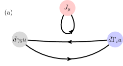
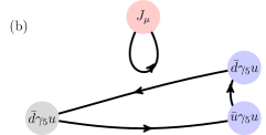
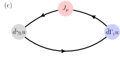
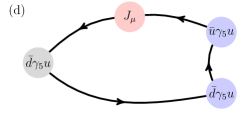
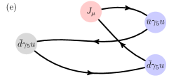
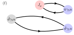
Figure 1: The different topologies of Wick contractions that make up the three-point function $C_{3,\;\mu,i}^{\vec{p}_{\pi},\,\vec{P},\,\Lambda,\,r}(t_{\pi},t_{J},t_{\pi\pi})$. The current-disconnected diagrams a) and b) are not included in the construction of the three-point functions.

The three-point functions as written in Eq. (4) are still a sum over all states in the $\pi\pi$ channel and need to be projected to the finite-volume states which have well-defined invariant mass $s$ and momentum transfer $q^{2}$. We achieve this by making use of the generalized eigenvectors $v_{i}^{n\,\vec{P},\Lambda}(t_{0})$ from the variational analysis in Ref. [6], and construct the optimized three-point functions [8, 9, 10]:

$$\Omega_{3,\;\mu,\,n}^{\vec{p}_{\pi},\,\vec{P},\,\Lambda,\,r}(t_{\pi},t_{J},t_{\pi\pi},t_{0})=v_{i}^{n\,\vec{P},\Lambda}(t_{0})\>C_{3,\;\mu,i}^{\vec{p}_{\pi},\,\vec{P},\,\Lambda,\,r}(t_{\pi},t_{J},t_{\pi\pi})$$ (6)

$$=\sqrt{2E_{n}^{\vec{P},\Lambda}}\,e^{E_{n}^{\vec{P},\Lambda}t_{0}/2}\,Z_{\pi}^{\vec{p}_{\pi}}\,\langle\pi,\vec{p}_{\pi}|J_{\mu}(0,\vec{q})|n,\vec{P},\Lambda,r\rangle_{FV}\times\frac{e^{-E_{\pi}^{\vec{p}_{\pi}}(t_{\pi}-t_{J})}e^{-E_{n}^{\vec{P},\Lambda}(t_{J}-t_{\pi\pi})}}{2E_{n}^{\vec{P},\Lambda}2E_{\pi}^{\vec{p}_{\pi}}}.$$ (7)

Here, the sum over all states $n$ in the irreducible representation is reduced to a single term which enables us to use all individual excited states within the energy region of interest to determine the matrix element at as many points as allowed by the quark masses and volume of the gauge ensemble.

The matrix elements $\langle\pi,\vec{p}_{\pi}|J_{\mu}(0,\vec{q})|n,\vec{P},\,\Lambda,\,r\rangle_{FV}$ are determined using the ratio

$$R_{\mu,\,n}^{\vec{p}_{\pi},\,\vec{P},\,\Lambda,\,r}(t_{\pi},t_{J},t_{\pi\pi})=\frac{|\langle\pi,\vec{p}_{\pi}|J_{\mu}(0,\vec{q})|n,\vec{P},\,\Lambda,\,r\rangle_{FV}|^{2}}{4E_{n}^{\vec{P},\Lambda}E_{\pi}^{\vec{p}_{\pi}}}$$ (8)

$$=\frac{\Omega_{3,\;\mu,\,n}^{\vec{p}_{\pi},\,\vec{P},\,\Lambda,\,r}(t_{\pi},t_{J},t_{\pi\pi},t_{0})\>\Omega_{3,\;\mu,\,n}^{\vec{p}_{\pi},\,\vec{P},\,\Lambda,\,r\,{\dagger}}(t_{\pi},t^{\prime},t_{\pi\pi},t_{0})}{C_{\pi}^{\vec{p}_{\pi}}(\Delta t)\>\lambda_{n}^{\vec{P},\Lambda}(\Delta t,t_{0})},$$ (9)

which depends on the optimized three-point functions as well as the two point functions.

4 Mapping to infinite volume

To obtain the infinite-volume matrix elements we follow the Briceño-Hansen-Walker-Loud approach [3, 4], which is a generalization of the seminal work of Lellouch and Lüscher [11] and allows us to utilize any gauge ensemble to study general transitions between single-hadron and two-hadron states. The mapping in the case of $\pi\gamma\to\pi\pi$ looks like

$$\frac{|\langle\pi,\vec{p}_{\pi}|J_{\mu}(0)|s,q^{2};\vec{P},\,\Lambda,\,r\rangle_{IV}|^{2}}{|\langle\pi,\vec{p}_{\pi}|J_{\mu}(0,\vec{q})|n,\vec{P},\,\Lambda,\,r\rangle_{FV}|^{2}}=\frac{1}{2E_{n}^{\vec{P},\Lambda}}\frac{16\pi\sqrt{s_{n}^{\vec{P},\Lambda}}}{k^{\vec{P},\Lambda}_{n}}\left(\frac{\partial\delta}{\partial E}+\frac{\partial\phi^{\vec{P},\Lambda}}{\partial E}\right)\bigg{|}_{E=E_{n}^{\vec{P},\Lambda}},\qquad$$ (10)

where $\phi^{\vec{P},\Lambda}$ are the combinations of the finite-volume quantization condition (cf. Eq. 49 of Ref. [6]) and $\delta$ is the scattering phase shift as determined in Ref. [6]. We make use of two different parametrizations of the scattering phase shift and perform the infinite-volume mapping for both. The systematic uncertainties associated with the different choices in fitting the energies and matrix elements are propagated to the final results.

5 The $\pi\gamma\to\pi\pi$ amplitude

We build the transition amplitude ${\cal V}_{\pi\gamma\to\pi\pi}$ (see Eq. 3) from phase shifts BW I and BW II and parametrize the transition form factor $F$ with a two-dimensional Taylor series:

$$F(q^{2},s)=\frac{1}{1-\frac{q^{2}}{m_{P}^{2}}}\sum_{n,m}A_{nm}z^{n}\mathcal{S}^{m},$$ (11)

where ${\cal S}=\frac{s-m_{R}^{2}}{m_{R}^{2}}$, $z=\frac{\sqrt{4m_{\pi}^{2}-q^{2}}-\sqrt{4m_{\pi}^{2}}}{\sqrt{4m_{\pi}^{2}-q^{2}}+\sqrt{4m_{\pi}^{2}}}$, and $m_{R}$ corresponds to the $\rho$ resonance mass. Because we neglect the current-disconnected diagrams, we also set $m_{P}=m_{R}$. We investigate three different systematic truncations: F1) combined order $K$, $\sum_{n+m\leq K}$, F2) order $N$ in $z$ and combined order $K$, $\sum_{n=0}^{N}\sum_{m=0}^{K-n}$, and F3) order $N$ in $z$ and order $M$ in $\mathcal{S}$, $\sum_{n=0}^{N}\sum_{m=0}^{M}$. We present a three-dimensional projection of the transition amplitude ${\cal V}_{\pi\gamma\to\pi\pi}$ for the chosen parametrization “BW II F1 K2” in Fig. 2.

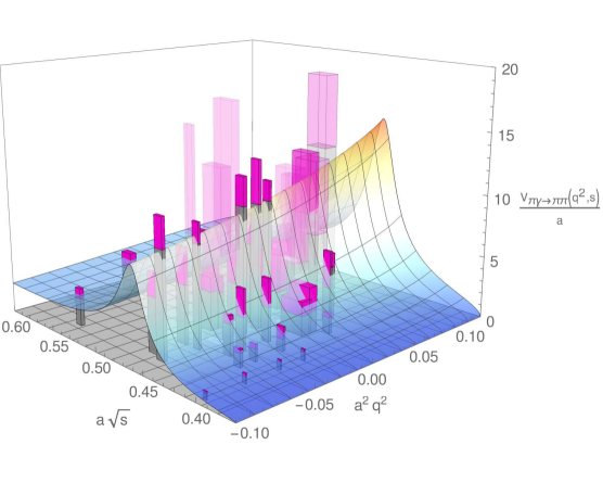
Figure 2: A three-dimensional plot of ${\cal V}_{\pi\gamma\to\pi\pi}$. The surface shows the central value of the nominal fit function (“BWII F1 K2”). The lattice results are shown as the vertical bars, with the widths and depths corresponding to the uncertainties. The magenta sections in the vertical direction cover the range from ${\cal V}_{\pi\gamma\to\pi\pi}-\sigma_{{\cal V}_{\pi\gamma\to\pi\pi}}$ to ${\cal V}_{\pi\gamma\to\pi\pi}+\sigma_{{\cal V}_{\pi\gamma\to\pi\pi}}$. Data points with larger uncertainties have reduced opacity.

6 Resonant form factor and photocoupling

The resonant form factor is determined by analytically continuing the transition form factor $F$ to the $\rho$ pole:

$$F_{\pi\gamma\to\rho}(q^{2})=F(q^{2},\,m_{R}^{2}+im_{R}\Gamma_{R}).$$ (12)

At zero momentum transfer, $q^{2}=0$, the resonant form factor becomes equal to the photocoupling $G_{\rho\pi\gamma}$, which enters the formula for the $\rho$ radiative decay width $\Gamma(\rho\to\pi\gamma)$:

$$\Gamma(\rho\to\pi\gamma)=\frac{2}{3}\alpha\left(\frac{m_{R}^{2}-m_{\pi}^{2}}{2m_{R}}\right)^{3}\frac{|G_{\rho\pi\gamma}|^{2}}{m_{\pi}^{2}}.$$ (13)

The left panel of Fig. 3 shows the resonant transition form factor as a function of momentum transfer. The inner shaded region corresponds to the statistical and systematical errors and the outer shaded region represents the model uncertainty, evaluated point-by-point as the root-mean-square deviation of the other parametrizations from the nominal parametrization.

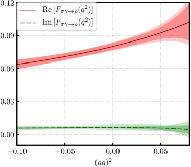
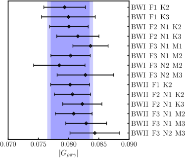
Figure 3: Left panel: Resonant transition form factor $F_{\pi\gamma\to\rho}$ as a function of momentum transfer. Right panel: Absolute value of the photocoupling for the various parametrizations under consideration.

The right panel of Fig. 3 shows the photocoupling determined from those parametrizations that lead to a good description of the data without redundant parameters. We find the $\rho$ photocoupling at $m_{\pi}\approx 320$ MeV to be: $|G_{\rho\pi\gamma}|=0.0802(32)(20)$. Because our lattice QCD calculation was performed at an unphysical pion mass, our thresholds are much closer to the resonances than in nature and thus our phase space is unphysical. However, if we assume the photocoupling to be pion-mass independent and use the physical values of hadron masses to have the proper thresholds, we find the radiative decay width $\Gamma(\rho\to\pi\gamma)\,=\,84.2(6.7)(4.3)\,{\rm keV}$. The number in the first bracket represents the combined statistical and systematical uncertainty and the second uncertainty is associated with the parametrization.

7 Conclusions

In this talk we presented a $(2+1)$-flavor lattice QCD calculation of the $\rho$ photoproduction process at $m_{\pi}\approx 320$ MeV. Because at this light-quark mass the $\rho$ is a resonance, we made use of the the Briceño-Hansen-Walker-Loud formalism to calculate the general $\pi\gamma\to\pi\pi$ transition amplitude at many discrete points in the kinematic space of $q^{2}$ and $\sqrt{s}$. Fitting a multitude of parametrizations to the data and analytically continuing them to the $\rho$ pole enabled us to determine the $\rho$ photocoupling and radiative decay width. Additional computations are needed to perform the continuum extrapolation and the chiral extrapolation to the physical point, where direct comparisons with experimental data are possible. The methods used in this work are also applicable to other electroweak processes with two hadrons in the final state, such as $B\to\rho(\to\pi\pi)\ell\bar{\nu}$ and $B\to K^{*}(\to K\pi)\ell^{+}\ell^{-}$.

References

- [1] R. Koniuk and N. Isgur, “Where Have All the Resonances Gone? An Analysis of Baryon Couplings in a Quark Model With Chromodynamics,” Phys. Rev. Lett. 44 (1980) 845.
- [2] D. Rönchen, M. Döring, H. Haberzettl, J. Haidenbauer, U. G. Meißner, and K. Nakayama, “Eta photoproduction in a combined analysis of pion- and photon-induced reactions,” Eur. Phys. J. A51 no.~6, (2015) 70, arXiv:1504.01643 [nucl-th].
- [3] R. A. Briceño, M. T. Hansen, and A. Walker-Loud, “Multichannel 1 2 transition amplitudes in a finite volume,” Phys. Rev. D91 no.~3, (2015) 034501, arXiv:1406.5965 [hep-lat].
- [4] R. A. Briceño and M. T. Hansen, “Multichannel 0 2 and 1 2 transition amplitudes for arbitrary spin particles in a finite volume,” Phys. Rev. D92 no.~7, (2015) 074509, arXiv:1502.04314 [hep-lat].
- [5] C. Alexandrou, L. Leskovec, S. Meinel, J. Negele, S. Paul, M. Petschlies, A. Pochinsky, G. Rendon, and S. Syritsyn, “ transition and the radiative decay width from lattice QCD,” Phys. Rev. D98 no.~7, (2018) 074502, arXiv:1807.08357 [hep-lat].
- [6] C. Alexandrou, L. Leskovec, S. Meinel, J. Negele, S. Paul, M. Petschlies, A. Pochinsky, G. Rendon, and S. Syritsyn, “-wave scattering and the resonance from lattice QCD,” Phys. Rev. D96 no.~3, (2017) 034525, arXiv:1704.05439 [hep-lat].
- [7] J. Green, N. Hasan, S. Meinel, M. Engelhardt, S. Krieg, J. Laeuchli, J. Negele, K. Orginos, A. Pochinsky, and S. Syritsyn, “Up, down, and strange nucleon axial form factors from lattice QCD,” Phys. Rev. D95 no.~11, (2017) 114502, arXiv:1703.06703 [hep-lat].
- [8] J. J. Dudek, R. Edwards, and C. E. Thomas, “Exotic and excited-state radiative transitions in charmonium from lattice QCD,” Phys. Rev. D79 (2009) 094504, arXiv:0902.2241 [hep-ph].
- [9] D. Becirevic, M. Kruse, and F. Sanfilippo, “Lattice QCD estimate of the ηc (2S) → J/ψγ decay rate,” JHEP 05 (2015) 014, arXiv:1411.6426 [hep-lat].
- [10] C. J. Shultz, J. J. Dudek, and R. G. Edwards, “Excited meson radiative transitions from lattice QCD using variationally optimized operators,” Phys. Rev. D91 no.~11, (2015) 114501, arXiv:1501.07457 [hep-lat].
- [11] L. Lellouch and M. Lüscher, “Weak transition matrix elements from finite volume correlation functions,” Commun. Math. Phys. 219 (2001) 31–44, arXiv:hep-lat/0003023 [hep-lat].