Cognition-inspired homeostasis can balance conflicting needs in robots

Abstract

Homeostasis keeps animals alive; it is a fundamental process that allows animals to adapt quickly to their environment. Artificial homeostasis can be used to help robots adapt to changing environments. Previous attempts at developing artificial homeostasis for robots were driven by mimicry of the biochemical machinery that drives homeostasis in humans. By considering homeostasis from a cognitive perspective, we develop a comparatively simple robot controller named CogSis (COGnitive HomeostaSIS) and demonstrate that it can provide homeostasis to a robot, even when there are conflicting needs. We present experiments showing that a robot running CogSis is able to learn from previous experiences and use them to influence future behaviour; can maintain its charge level while attending to another task (warming itself in an area separate from the charging station); and is able to maintain its charge level while avoiding a conflicting need (keeping cool, when the charging station is placed in a hot region of the environment). Results are presented in simulation and from a real robot platform.

Code for simulations and the robot controller are available at:
https://github.com/jstovold/CogSis_PythonSim/

1 Introduction

Homeostasis is a fundamental process in living beings, allowing our bodies to adapt to changes in the environment. The mechanisms to maintain the biochemical environment of the body have been studied at great length since 1878 when Claude Bernard observed that the internal environment (or ‘milieu interne’) was essential to survival (Bernard, 1878; Cannon, 1929).

Neal and Timmis (2003); Vargas et al. (2005) showed that the biological machinery for homeostasis could successfully be mimicked in a robot platform, laying the groundwork for future research in artificial homeostasis systems. The approach taken by Vargas et al. (2005) was to use a combination of artificial neural networks, endocrine networks, and immune systems to adapt the behaviour of a robot according to its internal environment. Stradner et al. (2009); Schmickl et al. (2011), on the other hand, use a combination of evolutionary algorithms and diffusion systems to mimic the hormonal changes within the human endocrine network, with similar success. While these approaches are effective, they often result in cumbersome architectures that are difficult to scale. The complicated systems used by Neal and Timmis (2003) and Vargas et al. (2005) are limited in how they can approach the complex problem of autonomous behaviour in robots.

While some changes induced by homeostasis are physiological (sweating, shivering etc.), some are behavioural changes. By altering our perception of the world around us, our behaviour is changed to help keep our internal environment within certain bounds (Widmaier et al., 2006), encouraging certain conscious actions and discouraging others. This is the cognitive view of homeostasis: the view that cognition is a highly-developed form of homeostasis (Lewontin, 1957; Ashby, 1960; Godfrey-Smith, 1998). In this paper, rather than viewing homeostasis as the result of interactions between the nervous, endocrine, and immune systems, we ask whether a system for artificial homeostasis can be built by taking inspiration from cognition.

This work represents a first step towards realising this view of altered perceptions. The robot controller and approach we present in this paper provide the ground work for more advanced cognitive experiments. Our approach is novel in that we consider the cognitive perspective of homeostasis, and demonstrate that this approach gives rise to a much simpler control architecture for homeostatic adaptive behaviour.

In section 2 we describe how we have adapted Cohen’s (2000) definition of distributed cognition into a robot controller, section 3 presents a series of experiments demonstrating the ability of the robot controller to balance conflicting needs, and so last longer in an environment without failing, in section 4 we discuss the impact of the work, and look forward to future research in this area, in particular considering how the architecture might be used to alter the perception of the world for various forms of robot. The appendix details the methods and experimental setup used for this work, including many specific details that are important but distracted from the overall message of the paper.

2 Implementing Cognitive Homeostasis

While discussing the cognitive nature of the immune system, Cohen (2000) proposes three properties of non-conscious cognitive systems:

“Cognitive systems, I propose, differ strategically from other systems in the way they combine three properties:

1. They can exercise options; decisions.

2. They contain within them images of their environments; internal images.

3. They use experience to build and update their internal structures and images; self-organization.” (p. 64, emphasis original)

The CogSis (COGnitive HomeostaSIS) system, shown in fig. 1, takes Cohen’s definition of immunological cognition and uses it as the basis for homeostasis in a robot. A robot running CogSis is able to perform basic cognitive tasks: making decisions, learning about the environment, and applying previous experience to influence future decisions. These cognitive tasks enable the robot to exhibit homeostatic behaviour and adapt to new environments rapidly, an ability not demonstrated by previous approaches (Vargas et al., 2005; Stradner et al., 2009).

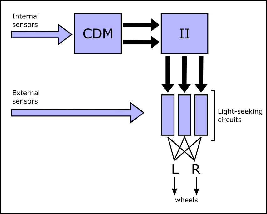
Figure 1: High-level architecture of the CogSis system. The internal sensors (battery charge, temperature) drive the behaviour of the cognitive decision making (CDM) module. As the virtual agents within the CDM react to the internal sensors, measuring the proportion of agents in each attractor source within the CDM can be used to drive the binary signals (black arrow) to the II’s (Internal Image) input. The II is implemented using a form of associative memory known as a Correlation Matrix Memory (CMM). This CMM is trained to recall which colour lamp is mounted above charging stations and high-temperature areas) then recalls which colour to search for according to the input that is triggered by the CDM. The output from the CMM is then fed into the light-seeking circuits that permit the robot to perform basic chromotaxis to seek out or flee from the appropriate colour in the environment.

CogSis consists of three main components: the CDM (Cognitive Decision Making) component, the II (Internal Image) component (implemented through a Correlation Matrix Memory), and some basic light-seeking circuitry. The CDM runs a novel decision-making algorithm (detailed in section 2.1), and provides action selection based on the robot’s internal sensor values.

Over the course of this section, we provide details of how each of Cohen’s components for cognition have been implemented. Each sub-section is split in two, with the first containing higher-level rationale and description of the approach, and the second sub-section providing the low-level implementation details required to fully understand the implementation and reproduce the work. Section 2.1 covers the decision-making component of CogSis, section 2.2 provides details of the internal memory of CogSis, and section 2.3 presents preliminary results showing how CogSis learns about its environment.

2.1 Decision Making

Cognitive systems are typically defined with decision making at the forefront (Cohen, 2000; Couzin, 2009; Visscher and Camazine, 1999; Trianni et al., 2011). Decision making is one of the key features of any intelligent system (Pfeifer and Scheier, 2001), which may explain its prevalence in definitions of cognition. The ability to change behaviour based on previous experience and the current situation allows for the wide repertoire of behaviours that typify cognitive systems (Pfeifer and Scheier, 2001). In this paper, we are predominantly interested in decentralised systems, especially those where the principles that are applied at the individual level can also scale to the group level. Consequently, the most appropriate form of decision making for us to use is collective decision making (Bose et al., 2017; McHugh et al., 2016; Marshall et al., 2017).

In order to prevent any prior interpretation of decision-making systems from clouding the behaviour of the decision-making algorithm implemented here, we define a collective decision-making system in a swarm of agents based directly on Cohen’s (2000) definition:

“[A] decision emerges…from a match between an environmental case and an internal motive. Decisions are associations. …Decision making is positive action; instead of passively receiving what the environment imposes, the cognitive system exerts its will…in choosing among alternatives” (p. 69)

This definition implies that for any given agent (e. g. a robot) to make a cognitive decision, it must be able to do more than simply react to the environment, it must be able to react differently to the same environmental cues based on its internal state.

We define the following terms:

• an agent is the entity making a decision, analogous to an ‘intelligent agent’ (Russell and Norvig, 2003). This could be an individual (e. g. a robot) or a collection (e. g. a swarm of virtual boids).

• the context is the state of the environment as perceived by an agent (Cohen’s ‘environmental case’).

• the motive is the likelihood of an agent picking a certain action should an appropriate context arise.

We can see that, in a cognitive system, an agent makes a decision based on some function of context and motive:

$$Decision=f(motive,context)$$

To illustrate how motive and context combine to produce decisions, we consider a simple case: a virtual agent in an empty simulated environment. The agent can move and can sense the environment around it; we argue here how context and motive could be implemented in such an artificial agent.

Let us first consider ‘context’: this is the current state of the environment as perceived by an agent. In the simplest case the agent is alone in an empty environment, meaning it should perceive nothing in the environment. If we introduce an artefact into the environment (for example, a simple attractor), then the agent will be able to perceive changes in its sensors depending on how close to the attractor it is. In our (otherwise empty) simulated environment, the attractor can represent one possible decision. We can interpret the agent moving towards the attractor as indicating a preference of the agent for the particular decision represented by the attractor.

Motive is the likelihood of picking an action based on the context. If the agent has the choice of two decisions, then it will pick whichever is closest unless the motive pushes it towards some other part of the environment. This motive could be as simple as momentum within the agent, but as we are interested in collective decision-making we opted for a flock of agents such that a form of ‘peer pressure’ would influence the decision making. This is achieved through the ‘motive’ force (see section 2.1.1 below for details).

Continuing with our example of the simple agent in an empty environment with attractors that represent possible decisions, the movement of the agent can be described by a combination of vector adjustments according to input from sensors (the ‘context’) and an internal driving force (the ‘motive’). By using vector adjustments, we are taking a similar approach to controlling the agent as that of Reynolds (1987).

The full details of how we calculate the vector adjustments, along with parameter values and testing are available in section 2.1.1. If you wish to skip the finer details then the next part of our artificial cognition is described in section 2.2.

2.1.1 Implementation Details

This section provides details of how the decision-making system is implemented, based on the high-level description provided above in section 2.1. The decision-making component of CogSis is used to decide which of the low-level signals should affect the high-level behaviour of the robot.

The decision-making component of CogSis uses a group of virtual agents collected into a flock in a virtual environment. The environment is predominantly empty, except for two attractors which provide the context for the flock of agents. The environment (and the flock within) will be simulated by the robot, and the actions of the flock within its virtual environment will provide decision making to the robot, based on the robot’s internal sensor values. each attractor in the environment is linked to a sensor on the robot, and the strength of its attraction (coefficient of attraction) is varied according to the value arriving from its corresponding sensor.

We have already seen in section 2.1 that a decision results from some function of motive and context, given the high-level definitions of what we would consider ‘context’ and ‘motive’. If the flock is placed into an empty environment, where there is no context, the actions of this flock can only result from the inherent predisposition of certain actions within the flock, and so—given the lack of context—must be representative of the motive of the flock.

As the values of the internal sensors in the robot vary, so do the associated attractors in the virtual environment. The flock of agents respond to changes in the virtual environment, linking the behaviour of this virtual flock to changes in the internal environment of the robot. The movement of the flock of agents between attractors, therefore, provides the action selection required for the high-level behaviour of the robot by reacting to the low-level sensor values. In this paper, the attractors are connected to the charge level and temperature sensors on the robot.

The layout of this virtual environment could be varied in a number of different ways, but—other than varying the strength of the attraction—we keep the environment static (dynamic environments is the subject of our ongoing research in this field). For this paper, we use an environment of 60x60 units with a periodic boundary condition. The attractors are centred at (30, 15) and (30, 45), with a spread of 7 units (see fig. 2). The flock of agents is initialised at (15, 30). Through the use of emergent identities (Stovold et al., 2014), multiple flocks could be supported in the same environment but this is outside the scope of this paper.

Figure 2: Screenshot of simulated decision-making environment embedded into the CDM module. Two attractors are shown in blue and red, representing the decision to charge and to avoid high temperatures, respectively. The flock of agents is moving towards the ‘avoid high temperatures’ attractor, and when more than half the agents are within 7 units of the centre, the CDM will notify the II module that the system should flee high temperatures.

There are many different flocking algorithms that could be used to control our group of agents, most famous of which is Reynolds’ boids (Reynolds, 1987). For this work, we picked a flocking algorithm that has a more rigid internal structure (Olfati-Saber, 2006), which allows the information from a contextual cue to more quickly propagate through the flock. this also helped to keep the flock cohesive over time, whereas Reynolds’ boids were more inclined to act as individuals, with the flock breaking up once they encounter an attractor.

The agents in the flock move according to three forces: the flock force, the motive force, and the context force. These three forces—described in detail below—combine to provide a final directional force that the agents follow. The flock force is provided by Olfati-Saber’s algorithm (Olfati-Saber, 2006), and works to keep the flock in a lattice formation. The motive force provides the ‘momentum’ within each agent, and works by projecting ‘virtual goals’ ahead of each agent in the flock. The context force provides environmental cues to the agents, resulting from the attractors in the environment.

Combining each of these three forces gives the overall algorithm, described by a series of vector adjustments, $u_{i}$, for an agent $i$:

$$u_{i}=f_{i}^{g}+f_{i}^{\gamma}$$ (1)

where $f_{i}^{g}$ acts to form a lattice structure among the neighbours in a flock (flock force), and $f_{i}^{\gamma}$ provides ‘navigational feedback’ towards a goal (combining motive and context forces). This definition of $u_{i}$ varies from Olfati-Saber’s (2006) original definition through the removal of the directional term $f_{i}^{d}$, relying instead on the navigational feedback provided through $f_{i}^{\gamma}$.

Flock force

The flock force, $f_{i}^{g}$, provides the cohesive force that pushes the agents into a lattice formation (Olfati-Saber, 2006). It is defined as:

$$f_{i}^{g}=-\nabla_{q_{i}}V(q)$$ (2)

where $V(q)$ is an attractive/repulsive force based on the distance to the nearest neighbouring agents, and $q_{i}$ is the two-dimensional position of agent $i$. $f_{i}^{g}$ provides the force required to keep an agent $i$ a set distance from its neighbouring agents. The full details of the flocking algorithm are provided in (Olfati-Saber, 2006).

By restricting the agents to only local interactions, the algorithm is applicable to both simulated and real (robotic) platforms. In order to provide $f_{i}^{\gamma}$ to the flock without global information, each agent projects a ‘virtual goal’ ahead of itself, which collectively provides the navigational feedback required to prevent the flock from disintegrating (Olfati-Saber, 2006). This virtual goal is the key component of the ‘motive force’.

Motive force

The motive force is provided through a ‘virtual goal’ in the environment. This is calculated by each agent projecting forward by a predetermined distance, d, and using that position in the environment as its goal for a set period of time, G${}^{\texttt{update}}$. These parameters, d and G${}^{\texttt{update}}$, are set at the start of each simulation run, and do not vary throughout the run or between agents. Between them, these parameters provide a weighting towards motive or context for the agents (i. e. a weighting between the motive force and the context force).

Specifically, an agent $i$ calculates its virtual goal, $G_{i}$, by taking the average heading of its neighbours, $N_{i}$, within a pre-defined radius, r. Let the average heading of the neighbours of agent $i$ be $\phi_{i}$, defined as:

$$\phi_{i}=\dfrac{1}{|N_{i}|}\sum_{j\in N_{i}}\theta_{j}$$ (3)

then projecting forwards by the predefined distance, d, gives the virtual goal for an agent $i$ as the coordinate pair $G_{i}=(x_{G_{i}},y_{G_{j}})$, providing the motive force $f_{i}^{motive}$:

$$x_{G_{i}}= \,x_{i}+d\cdot cos(\phi_{i})$$ (4)

$$y_{G_{i}}= \,y_{i}+d\cdot sin(\phi_{i})$$ (5)

The goal is recalculated periodically so that the motive reflects the current state of the agent, including influences from the environment. This update period is parameterised as the virtual goal update interval (G${}^{\texttt{update}}$). As the interval is increased, the agent is weighted further towards the motive than the context (and vice-versa), as information from the context will influence the position of the virtual goal less often.

Context force

The environment is empty other than any attractor sources included. An attractor, $j$, exerts a force on all agents in the environment. The force at any point can be described by the Gaussian probability density function, with mean $\mu_{j}$, standard deviation $\sigma_{j}$, and distance to the centre of the attractor from agent $i$, $(q_{i}-\mu_{j})$.

$$f_{i}^{context}(\mu_{j},\sigma_{j},q_{i})=\dfrac{1}{\sqrt{2\sigma_{j}^{2}\pi}}\,e^{-\dfrac{(q_{i}-\mu_{j})^{2}}{2\sigma_{j}^{2}}}$$ (6)

The agent calculates $f_{i}^{\gamma}$ based on the coordinates of $G_{i}$ and the gradient formed by the attractors in the environment:

$$f_{i}^{\gamma}=f_{i}^{motive}(q_{i},p_{i},q_{G_{i}},p_{G_{i}})+f_{i}^{context}(\mu_{j},\sigma_{j},q_{i})$$ (7)

Each agent multiplies the attractor gradient by a global parameter ctx$\_$mult as it senses it, in order to provide a weighting between $f_{i}^{motive}$ and $f_{i}^{context}$. See table 1 for a summary of each term used in the definition of $f_{i}^{\gamma}$.

Variable	Description
$q_{i}$	Two-dimensional position of agent $i$
$p_{i}$	Velocity of agent $i$
$G_{i}$	Position of virtual goal for agent $i$
$\mu_{j}$	Centre-point of attractor $j$
$\sigma_{j}$	Spread of attractor $j$

Table 1: Descriptions of the variables used in equation 7.

Parameter	Description	Value	Units
ctx$\_$mult	Multiplier for attractor gradient	185	N/A
d	Distance from agent to virtual goal	30	patches
G${}^{\texttt{update}}$	Update period for virtual goal	25	timesteps
r	Radius used to calculate neighbourhood	8	patches

Table 2: Typical parameter values and descriptions for the decision-making simulation. ‘Patches’ and ‘timesteps’ are generic terms for coordinate space in the simulation and discretised simulated time, respectively.

2.2 Internal Images / Memory

Cohen (2000) introduces memory through the concept of an ‘internal image’. This is a functional or physical imprint of the external environment on the cognitive system. These internal images provide a way for an otherwise blind system to interpret and interact with the outside world, translating from the internal ‘language’ of the cognitive system to actions in the external world. It is from this perspective that we have implemented memory in our system, to translate the decisions from the CDM module into actions in the real world. If the CDM module says ‘we need to charge’, the Internal Image (II) module recalls the last environmental cue in which the robot was charged. For example, if this was a blue light then the II module will output ‘seek out blue light’.

The II module lends itself well to associative memory: a mechanism for associating stimuli with responses. In biological systems, the memory results from temporal associations that emerge between two sets of interacting neurons (Palm, 1980, 1981). As the stimulus is presented to the first set of neurons, the response of those neurons is sent to the second set of neurons, which subsequently respond. This second response is similar every time, indicating that the same response will occur if given the same stimulus.

CMMs (Correlation Matrix Memories) (Kohonen, 1972) are one type of associative memory that have a particularly simple structure, a fast response time, and they can be trained in a single pass, meaning associations can be built up as the robot experiences new parts of the environment. These properties make them ideal for our purposes in the II module.

Section 2.2.1 provides an overview of CMMs along with details of how we use CMMs in the II module to translate between the internal language of the cognitive system and actions in the real world.

2.2.1 Implementation Details

In this section we introduce an overview of Correlation Matrix Memories (CMMs) and detail how they are used in the CogSis system through the internal image module.

The CMM (Correlation Matrix Memory) (Kohonen, 1972) is a matrix-based representation of a two-layer binary neural network. The matrix represents the binary weights from a fully-connected, two-layer artificial neural network (one input layer, one output layer; see fig. 3b). For example, the network in fig. 3b would be represented by the CMM, $\mathcal{M}$, with $k$ input–output pairs $\mathcal{I}$ and $\mathcal{O}$ in fig. 3a.

$$\begin{array}[]{lc|cr}\begin{matrix}\begin{pmatrix}~{}\\ \mathcal{I}\\ ~{}\end{pmatrix}&\begin{pmatrix}~{}&~{}&~{}\\ ~{}&\mathcal{M}&~{}\\ ~{}&~{}&~{}\end{pmatrix}\\ ~{}\\ &\begin{pmatrix}~{}&~{}\mathcal{O}&~{}~{}\end{pmatrix}\end{matrix}&{}{}\hfil&{}{}\hfil&\begin{matrix}\begin{pmatrix}a\\ b\\ c\end{pmatrix}&\begin{pmatrix}ad&ae&af\\ bd&be&bf\\ cd&ce&cf\end{pmatrix}\\ ~{}\\ &\begin{pmatrix}~{}d&~{}e&~{}f~{}\end{pmatrix}\end{matrix}\end{array}$$

(a) Basic CMM architecture (left), where $\mathcal{M}$ represents the matrix of binary weights, $\mathcal{I}$ and $\mathcal{O}$ represent the input–output vector pair corresponding to the neurons $a,b,c$ and $d,e,f$ in (b), respectively.

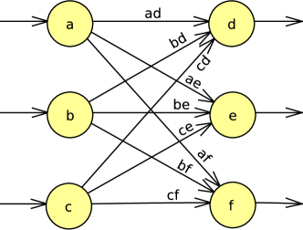
(b) CMM associative memory neural network. The binary weights between the two layers are represented by the matrix $\mathcal{M}$ in (a).

Figure 3:

Before training, the initial matrix $\mathcal{M}$ is filled with zeros (as there are no associations stored in the network). As the $k$ binary-valued input–output pairs are presented to the network, associations are built up in the matrix $\mathcal{M}$. These associations are stored as 1s in the matrix, corresponding to coincident 1s in both input and output vectors. For example, in fig. 3a, if $a$ and $e$ were both 1 then $ae$ would be set to 1 after training.

In the II module, we use a CMM to associate changes in the environment with changes in internal motive, following on from Cohen’s (2000) definition of cognitive decision-making:

“[A] decision emerges…from a match between an environmental case and an internal motive. Decisions are associations.” (p. 69)

He continues:

“Decision-making is positive action; instead of passively receiving what the environment imposes, the cognitive system exerts its will…in choosing among alternatives” (p. 69)

The associations made between the environmental case (referred to throughout this paper as ‘context’) and internal motive are made explicitly in the II module, but also implicitly in the CDM module described in section 2.1.

The output from the CDM module (i. e. the robot motive) is passed as an input to the CMM. In our system, the II module makes use of a CMM to store its ‘internal image’—or imprint—of the environment for the robot to use. The II, therefore, provides the robot with the capacity to make associations between changes in internal and external sensor values that occur at the same time. For example, if we mark a charging station with a blue light, the robot can sense the increase in blue light at the same time as an increase in battery charge. By associating these two signals, the II offers the ability to recall which colour to search for in order to find a charging station.

Fig. 4 shows how the II’s CMM is constructed for two internal sensors (charge, $c$, and temperature, $t$) and for the three colour components from an external light sensor (red, green, and blue). When one of the sensors passes a threshold, the corresponding binary value switches from 0 to 1. If this occurs on one of the internal sensors at the same time as one of the external sensors, then the corresponding value in the association matrix is set to 1 as well, storing this association between the two sensors. Re-presenting one of the internal sensor inputs (e. g. ‘charge’), by setting it to 1 again will recall the association. This will cause the closest stored associations to be recalled, and the appropriate values set in the output vector. This allows the system to test which colours have been associated with which inputs.

$$\begin{array}[]{lc|cr}\begin{matrix}\begin{pmatrix}c\\ t\end{pmatrix}&\begin{pmatrix}cr&cg&cb\\ tr&tg&tb\end{pmatrix}\\ ~{}\\ &\begin{pmatrix}~{}r&~{}g&~{}b~{}\end{pmatrix}\end{matrix}&{}{}\hfil&{}{}\hfil&\begin{matrix}\begin{pmatrix}1\\ 0\end{pmatrix}&\begin{pmatrix}~{}0&~{}0&~{}1\\ ~{}0&~{}0&~{}0\end{pmatrix}\\ ~{}\\ &\begin{pmatrix}~{}0&~{}0&~{}1~{}\end{pmatrix}\end{matrix}\end{array}$$

Figure 4: Basic CMM architecture (left), where $c$ and $t$ correspond to the internal sensors for charge and temperature, and $r$, $g$, and $b$ correspond to the red, green, and blue colour components from the light sensor, respectively. The vectors $\left(\begin{smallmatrix}c\\ t\end{smallmatrix}\right)$ and $(r\,g\,b)$ are provided as the stimulus–response pair of vectors to the association matrix. Any points in the association matrix that has a 1 on both input vectors is set to 1, storing the association between the two. An example association is shown on the right, as would occur after the robot finds a charging station under a blue light.

2.3 Self-organization / Learning

Cohen’s (2000) final property of cognitive systems is: “They use experience to build and update their internal structures and images; self-organization.” (p. 64). From Cohen’s viewpoint of immunological cognition, self-organization and learning look very similar, in fact he subsequently defines self-organization as:

“The hallmark of cognitive self-organization is the process we call learning; a cognitive system, through experience, acquires new capabilities and behaviors.” (Cohen, 2000, p. 82; emphasis original)

With this in mind, in this section we describe how the system can learn, and how it is set up to enable learning in new ways in future.

There are two main areas with the capacity to learn in the CogSis system: the II and the CDM. The II is the only area which we allow to learn for the work presented here, and the learning takes place through the association of internal needs and external sensor changes (i. e. when the robot is under a blue light and charging). This learning is sufficient for the work we are presenting in this paper, but there are other, more complex ways of learning in CogSis.

The CDM relies on the use of attractors that are linked to the internal sensors on the robot. With a fixed number of internal sensors (in this case temperature and charge), it was logical to fix the number of attractors in the virtual environment. There is, however, no reason why the CogSis system must be used in this way: we could link the CDM to a visual system which provides a much wider range of stimuli to the CDM. If this were the case, the argument for a dynamic virtual environment is much stronger. This is the focus of our current research efforts, but is far outside the scope of this paper.

2.3.1 Implementation Details

The CogSis system enables the robot to adapt to its environment through the use of the II’s CMM. The CMM associates large changes in internal sensor values with large changes in external sensor values. For example, if the robot discovers a charging station under a green lamp, the CMM will associate green light with charging. While, in principle, the CogSis system is able to adapt on-line, this functionality is disabled in all experiments presented in this paper. This ensures that any variation between test and control cases are only due to swapping out the CDM. This section aims to demonstrate that a robot running the CogSis system can learn from its experience in an environment, and put it into practice in a simulated environment ahead of being used in real robot experiments.

The simulation of our robot is shown in fig. 5. This simulation is constructed in NetLogo (Wilensky, 1999) and has the entire CogSis system implemented. The signals provided by the CDM to the rest of the system, however, are provided using switches on the simulator interface. The simulation consists of a single, zero-mass robot (a high-level representation of the real robot running CogSis) that roams around a simple environment with different coloured lights (red and green, in this case). In place of the CDM, we provide a mechanism for signalling that the robot has a certain need. This ‘need’ is usually provided by the decision-making ability of the CDM. By signalling that the robot has a certain need, the CogSis system provides a mechanism for the robot to find the corresponding part of the environment. For example, ‘needs charge’ recalls the appropriate colour of light from the CMM and searches for that colour in order to recharge.

Simulated training

The simulated robot roams around the environment during its training phase, learning about the environment. Once this has been completed the system is ready to be tested. In this case, if the training is successful, the robot should head towards the green light when the ‘needs charge’ motive is switched on.

Fig. 5 shows a trace of the simulated robot moving around the environment. Once the ‘needs charge’ switch is enabled (green arrow), the robot heads towards the green light source. Once this motive is disabled (blue arrow), the robot leaves the light source. This shows that, in principle, the system has the capacity to learn about its environment.

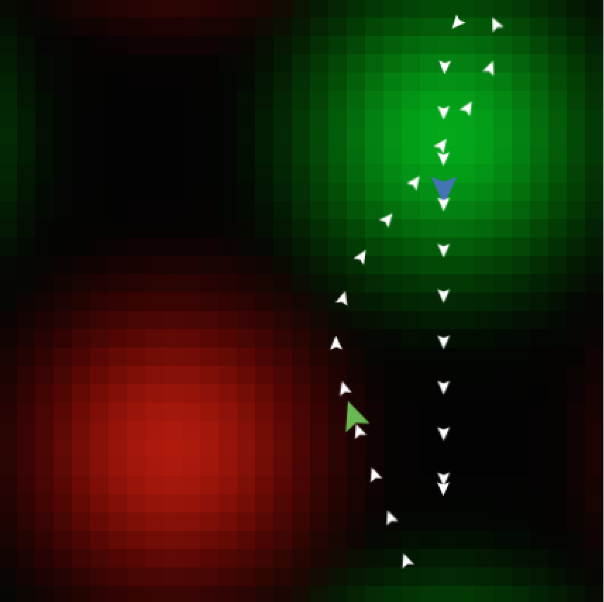
Figure 5: Screenshot of the proof-of-principle simulation, along with trace of the post-training robot searching for the green light source. The white arrows are the trace of the robot position, the green and blue arrows signify when the ‘needs charge’ motive switch is enabled and disabled.

The post-training behaviour of the simulation shows that the CogSis system is able to search for a specific part of the environment, based on high-level inputs such as a ‘needs charge’ signal. The system translates this signal back to a colour, based on previous experience of the environment. In other words, the system recalls ‘green’ as it learned that its batteries were charged when under a green light, which it subsequently seeks out.

Having shown that the system behaves as expected in a simulated environment, the next step is to implement this system on a hardware robot platform, and test whether this behaviour is consistent.

Robot-based training

The CogSis system is implemented onto a robot (details of the robot platform and experimental setup are provided in appendix A). As before, the robot is allowed to roam around the environment during its training phase, learning about the environment. The environment (shown in fig. 6) consists of two coloured lamps (one red, one blue), and the CogSis is set up to simulate charging its batteries under the blue light, and to simulate an increase in temperature under the red light.

As the robot roams, the CMM associates high values from the internal sensors with high values from the external sensors. Once the robot has roamed across both areas of the environment with lamps in, the robot is taken from the arena and the contents of the CMM downloaded.

Due to the small size of the CMM used in this paper (3x2 matrix), the training phase can be tested with relative ease. In the following matrices, the following key can be used to determine whether the training has been successful, $r,g,b$ correspond to the red, green, and blue external sensors, and $c,t$ correspond to the charge and temperature internal sensors:

$$\begin{matrix}\begin{pmatrix}cr&cg&cb\\ tr&tg&tb\end{pmatrix}\end{matrix}$$

After exposing the robot to an environment with one blue lamp over a charging station, the CMM is trained correctly as:

$$\begin{matrix}\begin{pmatrix}~{}0&~{}0&~{}1\\ ~{}0&~{}0&~{}0\end{pmatrix}\end{matrix}$$

After exposing the robot to an environment with both a red lamp over a high-temperature area and a blue lamp over a charging station, the CMM is trained correctly as:

$$\begin{matrix}\begin{pmatrix}~{}0&~{}0&~{}1\\ ~{}1&~{}0&~{}0\end{pmatrix}\end{matrix}$$

3 Results

By comparing with a control case, we demonstrate that CogSis can…

• …enable a robot to learn from previous experiences and use them to influence future behaviour

• …provide homeostatic behaviour to a robot

• …balance two conflicting requirements to provide homeostatic behaviour to a robot

This control case uses a replacement for the CDM that reacts to its internal state directly with a fixed threshold. The II and light-seeking circuits shown in fig. 1 are still present and functioning, and the CDM module still operates in order to take up the same CPU and memory time but without having any influence on the rest of the system.

3.1 CogSis provides homeostatic behaviour to a robot

This section considers how a robot running CogSis is able to alter its high-level behaviour according to its low-level needs. As the internal state of the robot varies, the CDM signals to the rest of the CogSis architecture what it needs in order to keep the state within its limits.

The CDM works to keep the internal sensors (charge and temperature) within certain limits. If the temperature gets too high or the charge too low then the robot will fail. The sensors are simulated so that the internal behaviour of the robot can be measured (if the battery actually ran out of charge, the data about internal behaviour might be lost or corrupted). The values used for different variables in our experimental setup are given in table 3.

	Temperature	Charge
Start value	10.0	5.0
+ve Delta	1.8	0.8
-ve Delta	0.5	0.1
Fail Point	–	0.1
Limits	[10.0, 60.0]	[0.01, 15.0]
Control threshold	–	2.5

Table 3: Parameter values used in the basic homeostasis experiment. The values have been picked to result in a challenging, but possible scenario.

This section looks at a basic scenario: asking whether the robot is able to keep itself charged while attending to another task. This other task is to warm itself under a lamp. By arranging the experimental arena (depicted in fig. 6) so that the charging station (a blue lamp) is far away from the warming lamp (a red lamp), the robot needs to leave the warming lamp in order to recharge, and vice-versa. This should result in the robot switching from sitting under one lamp to sitting under the other repeatedly and indefinitely. The parameters are chosen such that it is not able to warm itself sufficiently to complete its task before needing to charge again (thus cooling the robot back down again). This means that the robot will eventually run out of charge, but we are interested in how long the robot is able to balance the two tasks.

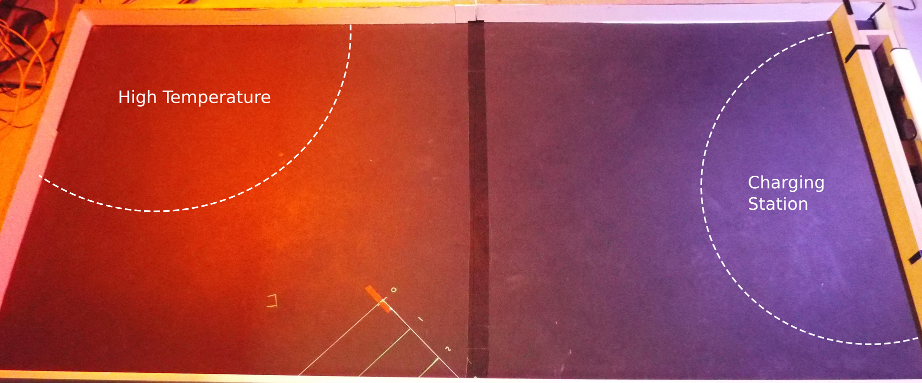
Figure 6: Photo of arena with charging and warm areas superimposed, arena size: 224x108cm

Null Hypothesis ($H_{0}$):

A robot running the CogSis architecture will survive no longer with the CDM component than with the threshold component.

The design of the system described in section 2 was such that the CDM could be replaced by another component that provides different signals, based on the values of the internal sensors. The control case uses a simple threshold mechanism to achieve this and provide a viable alternative to the CDM. The control output switches from 0 to 1 once the charge value drops below the control threshold of 2.5 (see appendix for calculation of appropriate control threshold values).

Due to the amount of time that robot lab experiments take, we constructed a simulated environment that mirrors the lab setup (see fig. 7a). Through this simulation, we are able to demonstrate the behaviour of the system in an idealised environment, before confirming the behaviour in a real-world lab setup. The simulation uses the same C++ code as the real robot, wrapped in Python and using Turtle graphics to represent the environment and robot. This code is available through the Github repository linked at the top of this article.

Fig. 7b shows the time for which a simulated robot is able to survive in the environment with the CDM and control setups. The data show a clear distinction between the CDM and control case, as supported by the statistical tests showing a significant difference between the distributions.

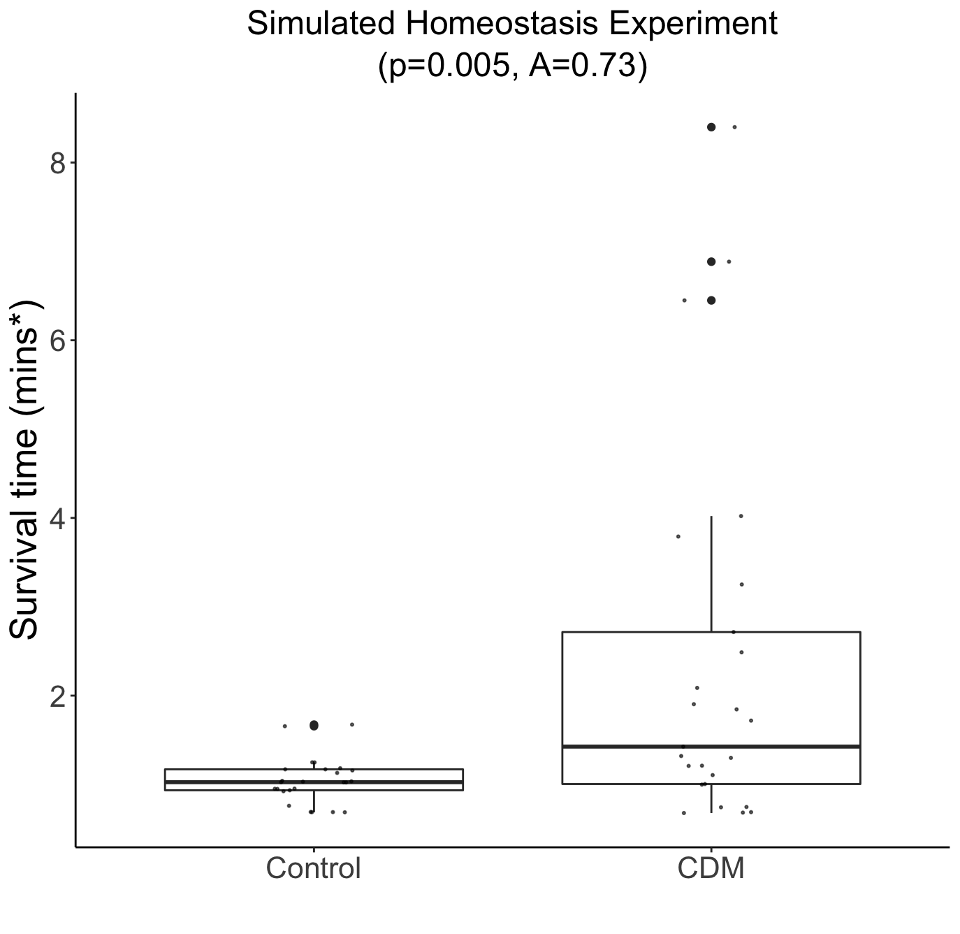
(a) Simulation environment, with white arrow representing the robot, blue light and red light representing the charging station and warming area, respectively.

(b) Boxplots showing that the CDM enables the robot to survive for significantly longer than a simple threshold controller (higher is better). The Mann–Whitney–Wilcoxon test and Vargha–Delaney A-test give $p=0.005$ and $A=0.73$ respectively, rejecting $H_{0}$ in simulation with 95% confidence.

Figure 7: Environment setup and results from simulated experiment (mimicking the real-world setup). N.B. the survival time is measured in minutes, but the simulation runs faster than the real robot, so the results are only proportionally comparable to the results gathered from real robots (presented below).

Fig. 8 shows the path of one run (a) with the CDM in place. The graph in (b) shows a subset of the internal sensor data provided to the CDM component for the duration of the experimental run. The robot was allowed to continue running until it reached 29 minutes, at which point it would be stopped. The traces show that the robot is able to perform a task while preventing itself from running low on charge.

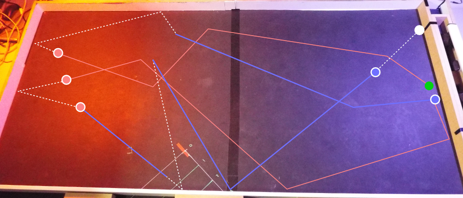
(a) Trace of robot path between 5.5 and 10.5 mins superimposed on the environment. The blue and red circles indicate points where the robot stopped to charge or warm itself respectively. The green and white circles indicate the start and end points. The red and blue solid lines indicate that the robot is searching for that colour. The white dotted line is when the robot wanders (not actively searching for anything).

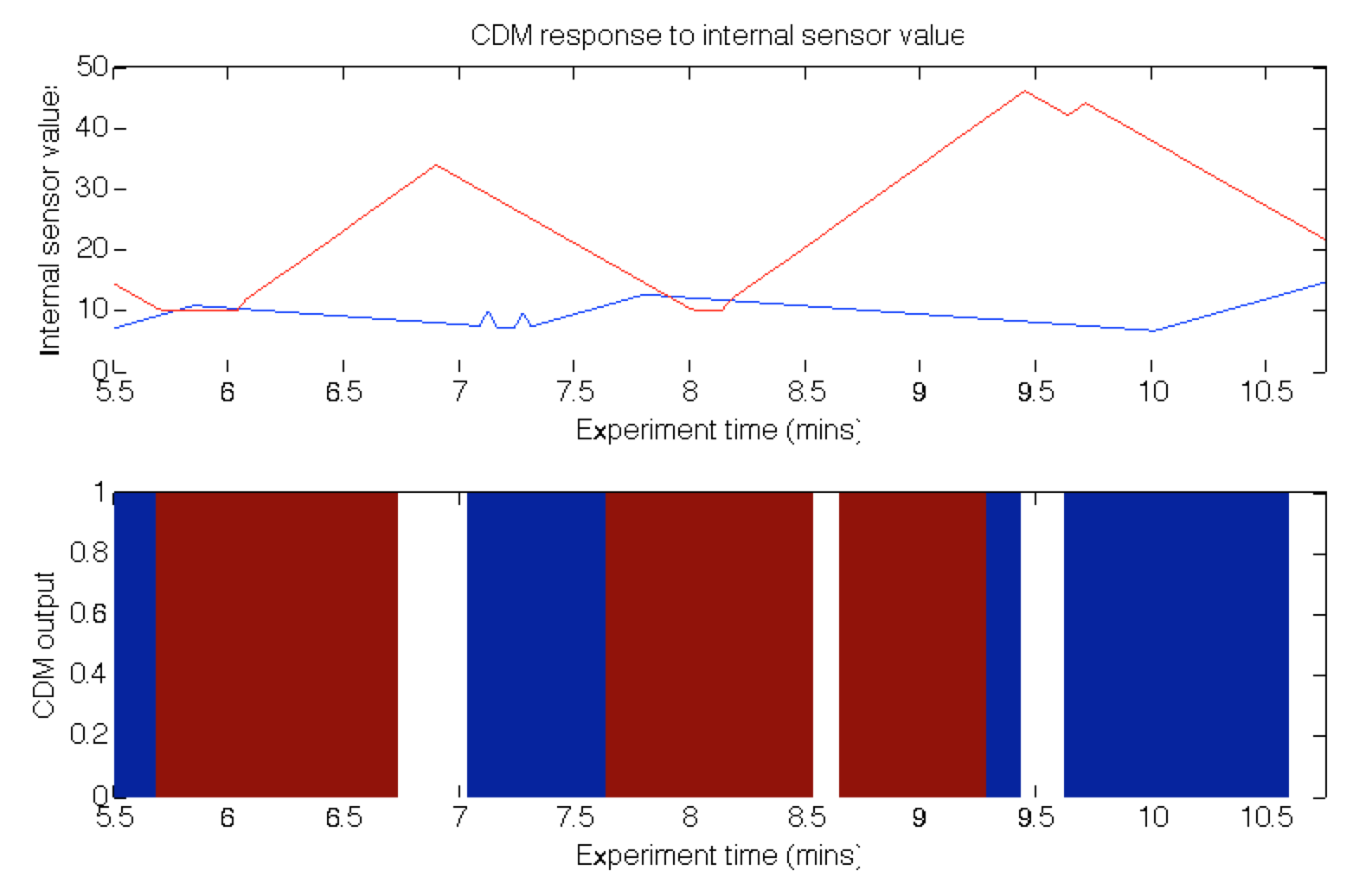
(b) Graphs showing internal sensor values (top) and CDM outputs (bottom) for the robot between 5.5 and 10.5 mins. The red and blue line show the internal values for temperature and charge as presented to the CDM component. The red and blue blocks of colour in the bottom graph show the output of the CDM component (red indicating to the robot to search for red light, and blue indicating to search for blue light).

Figure 8: A short (5 min) excerpt from one of the 29-minute replicates. The trace (a) shows how the robot moves between the red and blue areas in the environment as it needs to charge. The graphs in (b) show that as the internal sensor values for charge get too low, the robot actively searches for the charging station, and once it is charged sufficiently, it returns to warming itself under the red lamp.

Table 4 shows the length of time that the robot survived when set up with the two components described above (up to the maximum of 29 minutes). This data is presented in a table format, rather than a boxplot due to the relatively few replicates in this experiment. The high variance in the CDM data is unexpected and can be explained by the robot getting stuck in a corner early on in the run and failing as a result. These ‘failed’ runs are still included to ensure the results are not biased by their removal. Even with only 6 replicates, it is clear that the CDM code can survive for longer than the control code. This is confirmed through the Mann–Whitney–Wilcoxon test and Vargha–Delaney A-test, giving $p<0.05$ and $A>0.84$ respectively. From this, $H_{0}$ can be rejected at the 95% confidence level.

Replicate	Control (mins)	Test (mins)
1	3.5	29
2	4	2.5
3	2	29
4	2.5	6
5	10	29
6	3	29

Table 4: Details of how long the robot survived in the environment when using the CDM (test) component and the threshold (control) component. Mann–Whitney–Wilcoxon test and Vargha–Delaney A-test give $p<0.05$ and $A>0.84$ respectively, rejecting $H_{0}$ with 95% confidence.

While performing a relatively simple task, the results presented in this section show that the CogSis architecture is a viable option for providing simple artificial homeostasis to a robot. This provides the evidence required to answer the research question RQ2. The results here also suggest that the robot is able to make use of its previous experience in the environment, and apply it to survive in the same environment. This provides further evidence towards answering research question RQ1. The next section discusses how well the architecture handles more complicated scenarios that involve conflicting needs.

3.2 Conflicting decisions

While the work above shows how the CogSis system provides basic homeostatic behaviour to a robot, this section addresses research question RQ3: can the CogSis-controlled robot survive when faced with conflicting decisions about what to do?

Our experimental setup is altered to bring together the charging station and the higher temperature area (see fig. 9). The behaviour of the CDM is inverted with respect to temperature, so that the robot now tries to avoid getting warm. In order to charge its battery, therefore, the robot will have to endure warmer temperatures. Once the battery runs out, the robot will fail, and once the temperature reaches a set maximum, the robot will fail. This experiment once again makes use of the same architecture between test and control cases, except for the CDM component that will be replaced by the threshold component for the control case. As before, we use a simulated setup initially, and then verify the results using real robot tests.

Null Hypothesis ($H_{0}$):

A robot running the CogSis architecture will survive no longer with the CDM component than with the threshold component in the presence of conflicting needs.

The experimental setup is as shown in fig. 9. This is the same arena as above, except for the removal of the blue light from the right-hand side. In this more difficult scenario, the robot is expected to fail more often than it did in the previous setup, as before it was possible for the robot to sit and charge indefinitely without failing, whereas here this would result in a failure. After preliminary testing, it was evident that the parameter values used previously (given in table 3) provided a scenario that was too difficult for the robot to complete with either CDM or threshold-based architecture (all survival times were under 2.5 minutes). As such, the parameter values are adjusted to those shown in table 5, to make the robot less likely to overheat straight away, but balancing this by making it slower to charge.

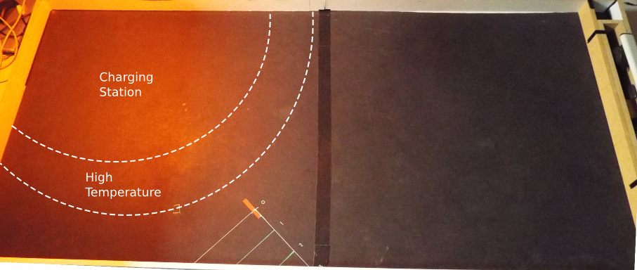
Figure 9: Photo showing the new arena for conflicting decisions experiment, arena size: 224x108cm

	Temperature	Charge
Start value	10.0	5.0
+ve Delta	1.3	0.3
-ve Delta	0.8	0.1
Fail Point	55.0	0.1
Limits	[10.0, 60.0]	[0.01, 15.0]
Control threshold	25.0	2.5

Table 5: The parameters used in the ‘conflicting decisions’ experiment. These values have been picked to result in a challenging, but possible scenario.

As with the experiment presented in section 3.1, we use a simulation to demonstrate the system behaves as expected without the need for long robot lab experiments. Fig. 10a shows the simulated environment, and fig. 10b shows the results of the test. It is clear from fig. 10b that the CDM outperforms the control case, as supported by the statistical tests showing a significant difference between the distributions.

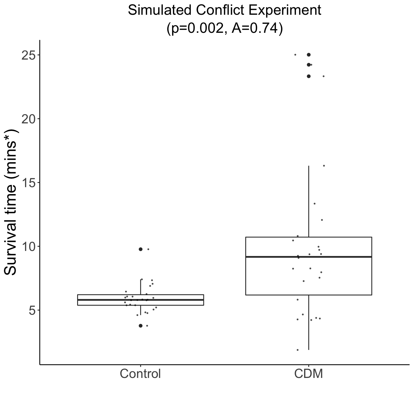
(a) Simulation environment with white arrow representing the robot and red light representing both the charging station and high temperature area.

(b) Boxplots showing that the CDM enables the robot to survive for significantly longer than a simple threshold controller when presented with conflicting decisions (higher is better). The Mann–Whitney–Wilcoxon test and Vargha–Delaney A-test give $p=0.002$ and $A=0.74$ respectively, rejecting $H_{0}$ in simulation with 95% confidence.

Figure 10: Environment setup and results from simulated experiment (mimicking the real-world setup). N.B. the survival time is measured in minutes, but the simulation runs faster than the real robot, so the results are only proportionally comparable to the results gathered from real robots (presented below).

Fig. 11 shows a trace of the sensor values as provided to the CDM component. The graphs show how the robot balances the need to charge its battery while avoiding getting too warm. The robot with CDM component was able to balance the conflicting decisions well, failing only once in 13 replicates, whereas the control case failed 6 times out of 13. These results are presented in full in table 6.

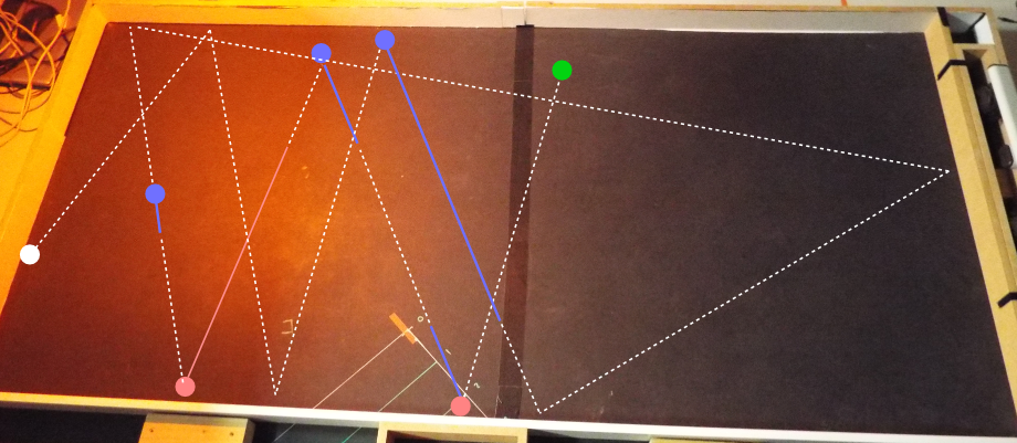
(a) Trace of robot path between 14 and 19 mins superimposed on the environment. The blue and red circles indicate points where the robot stopped to charge or cool itself respectively. The green and white circles indicate the start and end points. The blue and red solid lines indicate that the robot is searching for, or fleeing from, the red light, respectively. The white dotted line is when the robot wanders (not actively searching for anything).

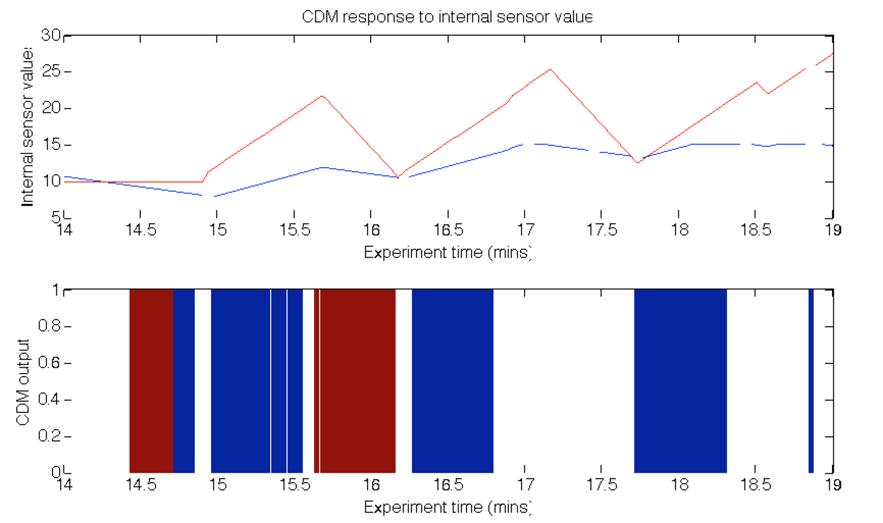
(b) Graphs showing internal sensor values (top) and CDM outputs (bottom) for the robot between 14 and 19 mins. The red and blue lines show the internal values for temperature and charge, as presented to the CDM component. The red and blue blocks of colour in the bottom graph show the output of the CDM component (red indicating to the robot to flee red light, and blue indicating to search for red light).

Figure 11: A short (5 min) excerpt from one of the 29-minute replicates. The trace (a) shows how the robot moves in and out of the red area in the environment as it needs to charge and cool down. The graphs in (b) show that as the internal sensor values for charge get too low, the robot actively searches for the charging station, and vice-versa for when the temperature gets too high. Note that, contrary to the behaviour described in fig. 8, when the temperature gets too high at around 17 mins, the CDM does not actively push the robot away from the red light, as it is already out of the area by chance. This has the effect of starting to reduce the temperature, reducing the likelihood that the CDM component would push the robot to seek out a cooler area.

Replicate	Control (mins)	Test (mins)
1	29	29
2	3	29
3	29	29
4	29	29
5	9	11
6	29	29
7	3	29
8	29	29
9	29	29
10	8	29
11	29	29
12	19	29
13	20	29

Table 6: Details of how long the robot survived in the environment when using the CDM (test) component and the threshold (control) component. Mann–Whitney–Wilcoxon test and Vargha–Delaney A-test give $p=0.03$ and $A=0.70$ respectively, rejecting $H_{0}$ with 95% confidence.

Table 6 show the amount of time that the two setups survived (up to the maximum of 29 minutes). There are 13 replicates for each. While these results were expected to be less clear-cut than the previous experiment, analysis gives similar results. The Mann–Whitney–Wilcoxon test gives $p=0.03$, and the Vargha–Delaney effect-magnitude test gives $A=0.70$. From this, $H_{0}$ can be rejected with $95\%$ confidence, resulting in the conclusion that the CDM component is better at balancing conflicting decisions than the threshold component, and providing sufficient evidence to answer research question RQ3. As with the previous experiment, the results here suggest that the robot is still able to make use of its previous experience in the environment, and apply it to survive in the same environment. This provides even further evidence towards answering research question RQ1.

4 Discussion and Future Work

This paper has presented a new approach to developing robotic homeostasis. By taking inspiration from cognition, rather than cellular-level biology, a simple homeostatic architecture has been developed for a robot which is able to balance conflicting needs. Evidence towards answering three research questions is presented. These research questions are summarised below.

RQ1 (Can CogSis enable a robot learn to from previous experiences and use them to influence future behaviour?) Section 2.3.1 presents the testing of the II training. This process consists of the robot roaming around an environment and associating simultaneous changes in the internal and external sensors. These associated changes represent the previous experiences that the robot has learnt. The behaviour of the robot in sections 3.1 and 3.2 show that the robot is able to successfully recall these experiences and use them to influence its high-level behaviour.

RQ2 (Can CogSis provide homeostatic behaviour to a robot?) Section 3.1 presents results showing that the robot is able to alter its high-level behaviour according to the value of two internal sensors (temperature and charge). The behaviour of the robot is compared between two versions of the CogSis architecture: one with the CDM component, one with a simple threshold function (see section 2). The CDM component consistently outperforms the threshold function at providing homeostatic behaviour to a robot, as shown by the survival task in fig. 8.

RQ3 (Can CogSis balance two conflicting needs to provide homeostatic behaviour to a robot?) Section 3.2 presents results showing that the robot is able to balance two conflicting needs. The robot was required to withstand a high-temperature region in order to gain access to a charging station. The behaviour of the robot is again compared between two versions of the CogSis architecture as with RQ2, above. The CDM component once again consistently outperforms the threshold function at providing homeostatic behaviour to a robot, while balancing two conflicting needs.

While other approaches to building artificial homeostasis have directly mimicked the natural systems of the body (Vargas et al., 2005; Stradner et al., 2009; Schmickl et al., 2011, Neal and Timmis, 2003; 2005), the CogSis architecture has been developed by taking inspiration from cognition (Cohen, 2000; Mitchell, 2005). Combining the CDM (cognitive decision making) with a CMM-based internal image module provides the CogSis (COGnitive HomeostaSIS) architecture with the ability to alter its high-level behaviour according to the low-level state of the robot, while based on previous experiences.

The CMM is trained by coincident ‘spikes’ in the internal and external sensors (e. g. when the ‘charge’ internal sensor rises at the same time as the ‘blue’ external sensor—this relates to a charging station under a blue light in the real-world environment). This provides adaptivity to the robot, as it is able to learn about new parts of an environment and adapt its behaviour accordingly (for example, if the robot were to find another charging station, it would store the association in the CMM and recall it as before).

The robot is able to make decisions about its current internal state through the CDM and transfer this to high-level behavioural changes, showing that the CogSis system provides the capacity for homeostasis to the robot. Furthermore, the use of the CMM to recall previous experiences allows the robot to proactively search for, or flee from, specific areas in the environment. This proactivity allows for behaviour that is more realistic for real-world applications.

The modular nature of the CogSis architecture, in that the CDM can be easily replaced by a different decision-making mechanism, makes the CogSis architecture more flexible for different applications. It could be possible to run multiple decision-making algorithms as an ensemble, with the combination of their outputs being passed to the CMM. Furthermore, there is a real possibility to extend this system to alter the perception of a robot based on the internal needs of the system. This would open up an interesting line of research where robots could be trained to focus their attention only on those parts of their immediate environment that relate to their current task, reducing the computational overhead required to solve tasks.

There is also potential for online learning about an environment, where the CMM would be training and recalling simultaneously. Furthermore, the sharing of experience between multiple robots working in the same area could be possible by sharing the contents of CMMs between robots.

In summary, cognition is a viable source of inspiration for homeostasis in robots. The resulting architecture shows that there is significant potential from implementing cognitive behaviour into robots, giving the ability to balance conflicting needs more effectively than a conventional threshold mechanism.

Appendix A Experimental Setup

The arena is 224x108cm with 15cm high boundaries (see the background of fig. 6). It has coloured LED lamps that can be moved so they point at different parts of the arena.

The robot platform is the Pi-Swarm (Hilder et al., 2014). This platform provides basic IR distance sensing and wheeled movement, along with colour LEDs on the top edge of the robot, and a simple speaker built-in. The robot is controlled using an ARM mbed LPC1768 chip (mbed, 2016) which runs custom C++ code. It has very limited flash and RAM storage, along with limited computational capacity. In order to provide information to the robot about the environment, the Pi-Swarm platform has a single RGB colour sensor (TCS3472) mounted on top.

LED lamps, mounted on tripods, provide a gradient of colour for the robot, using Perspex colour filters over the front in order to separate the different gradients. After initial analysis the best colours for this laboratory setup (in terms of other lights in the surrounding area and the contrast in the sensor) is a combination of the orange and yellow-green filters (referred to as ‘red’ throughout the paper for simplicity), or the blue filter.

For the purposes of this work, the robot makes use of two internal sensors: battery charge and temperature. These sensors are simulated, exploiting the fact that they are always beneath a lamp. As such, by setting the threshold for ‘detecting’ a charging station higher than the threshold for detecting the corresponding colour, the charging station is placed at the centre of the lamp’s gradient. The colour sensor returns values that are scaled according to the integration time and gain of the sensor (see (Adafruit Industries, 2012) for full details). The integration time and gain used for this experimental setup are 14.4ms and 60x, respectively. The colour sensor returns values based on the irradiance of its sensor, which is dependent on a wide range of environmental factors. The values used are proportional to lux, but it makes more sense to report values in terms of the relative responsivity of the sensor. For this reason, we define the ‘arbitrary colour unit’ (acu) as the value returned from the TCS3472 given an integration time of 14.4ms and gain of 60.

The threshold value for the control case was calculated from the amount of time it takes for the robot to get to the light source it is searching for. This was determined empirically as 45 seconds (the upper quartile of the data represented by fig. 12). Using this value for traversing the environment, the threshold can be calculated as 2.0. In order to take into account the variability of working in a noisy environment, the threshold was increased slightly to 2.5, allowing 54 seconds in the worst case for the robot to find its way between light sources. This also helps to reduce the chance of a false positive result by making it easier for the control setup to survive for longer.

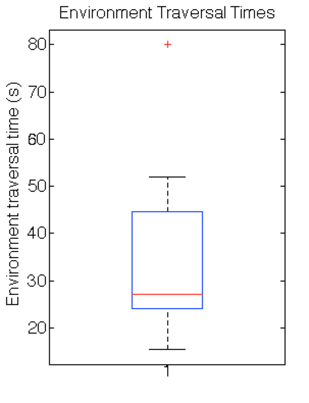
Figure 12: Boxplot showing how long it takes to cross the arena between light sources, measured empirically.

Parts of the work presented in this article was undertaken during JHS’ PhD (Stovold, 2016), funded by an EPSRC Doctoral Training Grant while at the University of York. A copy of JHS’ thesis is available through the White Rose eTheses Online portal.

The authors declare that there is no conflict of interest.

References

- Adafruit Industries (2012) Adafruit Industries (2012). Color Light-To-Digital Converter with IR Filter. ams.
- Ashby (1960) Ashby, W. (1960). Design for a brain: The origin of adaptive behaviour. Chapman and Hall, London.
- Bernard (1878) Bernard, C. (1878). Les phénomènes de la vie. Bailliere, Paris, 879:1.
- Bose et al. (2017) Bose, T., Reina, A., and Marshall, J. A. (2017). Collective decision-making. Current Opinion in Behavioral Sciences, 16:30–34.
- Cannon (1929) Cannon, W. B. (1929). Organization for physiological homeostasis. Physiological Reviews, IX(3):399–431.
- Cohen (2000) Cohen, I. R. (2000). Tending Adam’s Garden: evolving the cognitive immune self. Academic Press.
- Couzin (2009) Couzin, I. D. (2009). Collective cognition in animal groups. Trends in Cognitive Sciences, 13(1):36–43.
- Godfrey-Smith (1998) Godfrey-Smith, P. (1998). Complexity and the Function of Mind in Nature. Cambridge Studies in Philosophy and Biology. Cambridge University Press.
- Hilder et al. (2014) Hilder, J., Naylor, R., Rizihs, A., Franks, D., and Timmis, J. (2014). The Pi Swarm: A low-cost platform for swarm robotics research and education. In Mistry, M., Leonardis, A., Witkowski, M., and Melhuish, C., editors, Advances in Autonomous Robotics Systems, volume 8717 of Lecture Notes in Computer Science, pages 151–162. Springer International Publishing.
- Kohonen (1972) Kohonen, T. (1972). Correlation matrix memories. Computers, IEEE Transactions on, C-21(4):353 –359.
- Lewontin (1957) Lewontin, R. C. (1957). The adaptations of populations to varying environments. Cold Spring Harbor Symposia on Quantitative Biology, 22:395–408.
- Marshall et al. (2017) Marshall, J. A., Brown, G., and Radford, A. N. (2017). Individual confidence-weighting and group decision-making. Trends in Ecology & Evolution, 32(9):636–645.
- mbed (2016) mbed (2016). mbed LPC1768. Online: https://developer.mbed.org/platforms/mbed-LPC1768/.
- McHugh et al. (2016) McHugh, K. A., Yammarino, F. J., Dionne, S. D., Serban, A., Sayama, H., and Chatterjee, S. (2016). Collective decision making, leadership, and collective intelligence: Tests with agent-based simulations and a field study. The Leadership Quarterly, 27(2):218–241.
- Mitchell (2005) Mitchell, M. (2005). Self-awareness and control in decentralized systems. Metacognition in Computation, pages 80–85.
- Neal and Timmis (2003) Neal, M. and Timmis, J. (2003). Timidity: A useful emotional mechanism for robot control? Informatica, 27(2):197–204.
- Neal and Timmis (2005) Neal, M. and Timmis, J. (2005). Once more unto the breach…towards artificial homeostasis? In De Castro, L. N. and Von Zuben, F. J., editors, Recent Developments in Biologically Inspired Computing. Idea Group Pub.
- Olfati-Saber (2006) Olfati-Saber, R. (2006). Flocking for multi-agent dynamic systems: algorithms and theory. Automatic Control, IEEE Transactions on, 51(3):401–420.
- Palm (1980) Palm, G. (1980). On associative memory. Biological Cybernetics, 36(1):19–31.
- Palm (1981) Palm, G. (1981). Towards a theory of cell assemblies. Biological Cybernetics, 39(3):181–194.
- Pfeifer and Scheier (2001) Pfeifer, R. and Scheier, C. (2001). Understanding Intelligence. MIT Press, Cambridge, MA, USA.
- Reynolds (1987) Reynolds, C. W. (1987). Flocks, herds and schools: A distributed behavioral model. In Proceedings of the 14th annual conference on Computer graphics and interactive techniques, SIGGRAPH ’87, pages 25–34.
- Russell and Norvig (2003) Russell, S. J. and Norvig, P. (2003). Artificial Intelligence: A Modern Approach. Pearson Education, 2 edition.
- Schmickl et al. (2011) Schmickl, T., Hamann, H., and Crailsheim, K. (2011). Modelling a hormone-inspired controller for individual- and multi-modular robotic systems. Mathematical and Computer Modelling of Dynamical Systems, 17(3):221–242.
- Stovold (2016) Stovold, J. (2016). Distributed Cognition as the Basis for Adaptation and Homeostasis in Robots. PhD thesis, University of York.
- Stovold et al. (2014) Stovold, J., O’Keefe, S., and Timmis, J. (2014). Preserving swarm identity over time. In Sayama, H., Rieffel, J., Risi, S., Doursat, R., and Lipson, H., editors, Proceedings of the 14th international conference on the synthesis and simulation of living systems (ALIFE ’14), pages 728–735.
- Stradner et al. (2009) Stradner, J., Hamann, H., Schmickl, T., and Crailsheim, K. (2009). Analysis and implementation of an artificial homeostatic hormone system: A first case study in robotic hardware. In 2009 IEEE/RSJ International Conference on Intelligent Robots and Systems, pages 595–600.
- Trianni et al. (2011) Trianni, V., Tuci, E., Passino, K., and Marshall, J. (2011). Swarm cognition: an interdisciplinary approach to the study of self-organising biological collectives. Swarm Intelligence, 5:3–18.
- Vargas et al. (2005) Vargas, P., Moioli, R., Castro, L. N., Timmis, J., Neal, M., and Zuben, F. J. (2005). Artificial homeostatic system: A novel approach. In Capcarrère, M. S., Freitas, A. A., Bentley, P. J., Johnson, C. G., and Timmis, J., editors, Advances in Artificial Life: 8th European Conference, ECAL 2005, Canterbury, UK, September 5-9, 2005 Proceedings, pages 754–764. Springer Berlin Heidelberg, Berlin, Heidelberg.
- Visscher and Camazine (1999) Visscher, P. K. and Camazine, S. (1999). Collective decisions and cognition in bees. Nature, 397(6718):400–400.
- Widmaier et al. (2006) Widmaier, E. P., Raff, H., and Strang, K. T. (2006). Vander’s human physiology, volume 5. McGraw-Hill New York, NY.
- Wilensky (1999) Wilensky, U. (1999). NetLogo. http://ccl.northwestern.edu/netlogo/ Center for Connected Learning and Computer-Based Modelling, Northwestern University, Evanston, IL.