Generalized Range Moves

Abstract

We consider move-making algorithms for energy minimization of multi-label Markov Random Fields (MRFs). Since this is not a tractable problem in general, a commonly used heuristic is to minimize over subsets of labels and variables in an iterative procedure. Such methods include $\alpha$-expansion, $\alpha\beta$-swap and range-moves. In each iteration, a small subset of variables are active in the optimization, which diminishes their effectiveness, and increases the required number of iterations. In this paper, we present a method in which optimization can be carried out over all labels, and most, or all variables at once. Experiments show substantial improvement with respect to previous move-making algorithms.

1 Move-making algorithms

Generally speaking, multi-label MRF problems are more difficult than boolean label problems, and except in some specific cases (for example submodular problems) [9, 16] it is intractable to find an optimal solution. In this paper, we shall examine the underlying strategy behind move-making algorithms, to which such algorithms as $\alpha$-expansion, $\alpha\beta$-swap [6] and range-swap [17] belong. Later, we propose two extensions to the range-swap algorithm that enable the optimization to be carried out over all labels and most, or all variables at once. In our experiments, these generalizations clearly outperformed previous move-making algorithms for MRFs with robust non-convex priors such as, truncated quadratic and Cauchy function.

Consider a multi-label MRF defined by a cost function of the sort

$$E(\mathbf{x})=\sum_{i\in\mathcal{V}}E_{i}(x_{i})+\sum_{(i,j)\in\mathcal{E}}E_{ij}(x_{i},x_{j})\ ,\vspace{-0.1cm}$$ (1)

where $\mathbf{x}=\{\mathbf{x}_{i}~{}|~{}i\in\mathcal{V}\}$ (for some index set $\mathcal{V}=\{1,\ldots,N\}$, sometimes called vertices or nodes) and each $x_{i}$ is a variable taking values in an ordered label set $\mathcal{L}=\{0,1,\ldots,\ell-1\}$. Pairwise terms are defined for pairs of variables (sometimes called edges) indexed by $\mathcal{E}\subset\mathcal{V}\times\mathcal{V}$.

As an approach to minimizing energy function $E(\mathbf{x})$ of this kind, a move-making algorithm considers an MRF with labels $u_{i}$ in smaller label sets $\mathcal{L}_{i}^{\prime}$. Thus, $u_{i}\in\mathcal{L}_{i}^{\prime}$ for $i\in\mathcal{V}$. For each $i$, the value of $u_{i}$ determines a variable $x_{i}$ defined by a choice function

$$x_{i}=\phi_{i}(u_{i})\ ,$$ (2)

where $u_{i}\in\mathcal{L}^{\prime}$ and $x_{i}\in\mathcal{L}$. A common situation (for instance $\alpha$-expansion, $\alpha\beta$-swap) is where $\mathcal{L}^{\prime}_{i}=\mathcal{B}=\{0,1\}$. In other situations (for example, range-moves) each $\mathcal{L}^{\prime}_{i}$ is a fixed subset of $\mathcal{L}$. In Veksler’s range-swap algorithm [17], $\mathcal{L}^{\prime}_{i}=\mathcal{L}_{\alpha\beta}=\{\alpha,\alpha+1,\ldots\beta\}$ for some $\alpha,\beta\in\mathcal{L}$ with $\alpha<\beta$.

Each function $\phi_{i}$ defines the choice between various possible labels $x_{i}\in\mathcal{L}$, depending on the value of a “choice” variable $u_{i}$. Putting these all together, for all $i$, results in $\mathbf{x}=\phi(\mathbf{u})$, which is a function $\mathcal{L}^{\prime}_{1}\times\ldots\times\mathcal{L}^{\prime}_{N}\rightarrow\mathcal{L}^{\mathcal{V}}$ where each value $x_{i}$ depends on the value of the corresponding $u_{i}$. For simplicity, and with some apparent loss of generality, we shall write $\mathcal{L}^{\prime\mathcal{V}}$ instead of $\mathcal{L}^{\prime}_{1}\times\ldots\times\mathcal{L}^{\prime}_{N}$, but keep in our mind that each of the $\mathcal{L}^{\prime}_{i}$ may potentially be different.

Then, one may define a new cost function $E^{\prime}:\mathcal{L}^{\prime}{}^{\mathcal{V}}\rightarrow\rm I\!R$ by

$$E^{\prime}(\mathbf{u})=E(\phi(\mathbf{u}))\ .$$ (3)

In a move-making algorithm, the cost function $E^{\prime}(\mathbf{u})$ is minimized over all choices of $\mathbf{u}\in\mathcal{L}^{\prime}{}^{\mathcal{V}}$, and the resulting multi-label variable $\mathbf{x}^{*}=\phi(\mathbf{u}^{*})$ is assigned as the value of the variable $\mathbf{x}$. A complete algorithm applies a sequence of such moves. The typical move-making algorithm is set up as in Algorithm 1.

Algorithm 1 A move-making algorithm

$\mathbf{x}^{0}$ $\triangleright$ Initial assignment

repeat

     Choose $\phi^{t}:\mathcal{L}^{\prime}{}^{\mathcal{V}}\rightarrow\mathcal{L}^{\mathcal{V}}$ such that $\phi^{t}(\mathbf{u})=\mathbf{x}^{t}$ for some $\mathbf{u}$. $\triangleright$ Choice function

     $\mathbf{x}^{t+1}\leftarrow\phi^{t}(\mathbf{u}^{*})$ where $\mathbf{u}^{*}\leftarrow\operatorname{argmin}_{\mathbf{u}\in\mathcal{L}^{\prime\mathcal{V}}}E(\phi^{t}(\mathbf{u}))$ $\triangleright$ Update labelling

until $E(\mathbf{x}^{t+1})$ cannot be decreased any further

Note that because of the condition that $\phi^{t}(\mathbf{u})=\mathbf{x}^{t}$ for some value of $\mathbf{u}$, the cost $E(\mathbf{x})$ cannot increase as a result of the minimization step. If $\phi^{t}(\mathbf{u})=\mathbf{x}^{t}$, then

$$E(\mathbf{x}^{t+1})=E(\phi^{t}(\mathbf{u}^{*}))\leq E(\phi^{t}(\mathbf{u}))=E(\mathbf{x}^{t})\ .$$ (4)

This described the general move-making algorithm. Various examples of this algorithm will now be described, differing only in the choice of the functions $\phi^{t}(\mathbf{u})$. It is important to realize that these algorithms do not in general lead to an exact minimum for the multi-label optimization problem. However, in some cases, bounds on the obtained solution can be proved [6]. In practice, moreover, move-swapping algorithms can be demonstrated to work well.

1.1 Standard range moves

Veksler [17] suggested a method of range moves for solving non-submodular multi-label problems, specifically energy functions with truncated convex priors, as will be explained next.

Truncated convex optimization.

We wish to minimize an energy function $E^{g}(\mathbf{x})$, for $\mathbf{x}\in\mathcal{L}^{\mathcal{V}}$, with edge terms of the form

$$E^{g}_{ij}(x_{i},x_{j})=g(x_{i}-x_{j})\ ,$$ (5)

where $g$ is a function, known as the prior, which is assumed to be convex on the interval $[-T,T]$, but not convex over its whole domain. The particular case we are most interested in is the truncated quadratic energy function: $g(x)=\min(x^{2},T^{2})$. However, the algorithm to be discussed applies to a wider range of priors, such as the Cauchy function: $g(x)=T^{2}/2\log(1+(x/T)^{2})$ [8], as well as any function where a convex part is followed by a concave part. A convex (and hence submodular) prior without truncation may be optimized exactly with Ishikawa’s algorithm [9, 16] whereas with truncation, the problem is NP-hard, according to [6].

Let $\alpha,\beta\in\mathcal{L}$ be two labels such that $0<\beta-\alpha\leq T$ and define $\mathcal{L}^{\prime}_{i}=\mathcal{L}_{\alpha\beta}=\{\alpha,\ldots,\beta\}$. Given a labelling $\mathbf{x}^{t}$, a new labelling $\mathbf{x}^{t+1}=\phi(\mathbf{u})$, where $\mathbf{u}\in\mathcal{L}_{\alpha\beta}^{\mathcal{V}}$, is defined by

$$x^{t+1}_{i}=\phi_{i}(u_{i})=\left\{\begin{array}[]{l l}u_{i}&\mbox{~{} if ~{}}x_{i}^{t}\in\mathcal{L}_{\alpha\beta}\\ x_{i}^{t}&\mbox{~{} otherwise}\ .\\ \end{array}\right.$$ (6)

Hence, if a variable currently has its label in $\mathcal{L}_{\alpha\beta}$, then it has the possibility of changing to any other label in $\mathcal{L}_{\alpha\beta}$, according to the value of $u_{i}$. Such variables are known as the active variables. Nodes with labels not in $\mathcal{L}_{\alpha\beta}$ remain unchanged – the variable $x_{i}$ is inactive. Thus, defining $\mathcal{V}_{\,\alpha\beta}^{t}$ by

$$\mathcal{V}_{\,\alpha\beta}^{t}=\{i\in\mathcal{V}~{}|~{}x^{t}_{i}\in\mathcal{L}_{\alpha\beta}\}\ ,$$ (7)

the active variables are those $x_{i}$ with $i\in\mathcal{V}_{\,\alpha\beta}^{t}$. Denote, also, by $\mathcal{E}_{\,\alpha\beta}^{t}$ the set of edges $(i,j)$ joining two nodes in $\mathcal{V}_{\,\alpha\beta}^{t}$. A multi-label cost function $E^{\prime}(\mathbf{u})=E^{g}(\phi(\mathbf{u}))$ can now be defined. In the function $E^{\prime}:\mathcal{L}_{\alpha\beta}^{\mathcal{V}}\rightarrow\rm I\!R$ only those variables $u_{i}$ with $i\in\mathcal{V}_{\,\alpha\beta}^{t}$ are active; it may be thought of as a restriction of $E^{g}(\mathbf{x})$ to variables in $\mathcal{V}_{\,\alpha\beta}^{t}$, and to labels $\mathcal{L}_{\alpha\beta}$.

We wish to use Ishikawa’s algorithm for minimizing $E^{\prime}(\mathbf{u})$. The requirement for this is that $E^{\prime}$ should be submodular, more particularly, it should be defined by a convex prior on the label set $\mathcal{L}_{\alpha\beta}$.

It is easily verified that the unary terms in $E^{g}(\mathbf{x})$ lead to unary terms in $E^{\prime}(\mathbf{u})$. Let us consider the binary terms. Several cases arise.

1. If $x^{t}_{i}\not\in\mathcal{L}_{\alpha\beta}$ and $x^{t}_{j}\not\in\mathcal{L}_{\alpha\beta}$, then for all $(u_{i},u_{j})$,

   $$E^{\prime}_{ij}(u_{i},u_{j})=E^{g}_{ij}(\phi_{i}(u_{i}),\phi_{j}(u_{j}))=E^{g}_{ij}(x^{t}_{i},x^{t}_{j})\ ,\vspace*{-0.1cm}$$ (8)

   which is constant, with respect to the variables $\mathbf{u}$, and may be ignored.

2. If $x^{t}_{i}\in\mathcal{L}_{\alpha\beta}$ and $x^{t}_{j}\not\in\mathcal{L}_{\alpha\beta}$, then

   $$E^{\prime}_{ij}(u_{i},u_{j})=E^{g}_{ij}(u_{i},x^{t}_{j})\ ,\vspace*{-0.1cm}$$ (9)

   which is a unary term, depending only on $u_{i}$.

3. If $x^{t}_{i},x^{t}_{j}\in\mathcal{L}_{\alpha\beta}$, then

   $$E^{\prime}_{ij}(u_{i},u_{j})=E^{g}_{ij}(u_{i},u_{j})=g(u_{i}-u_{j})\ .$$ (10)

   However, $|u_{i}-u_{j}|\leq T$, since both $u_{i}$ and $u_{j}$ are in $\mathcal{L}_{\alpha\beta}$. Therefore, $u_{i}-u_{j}$ lies in the range $[-T,T]$ on which $g$ is convex. Therefore, the term $E^{\prime}_{ij}$ is defined by a convex prior in terms of the labels $\mathcal{L}_{\alpha\beta}$, and is therefore submodular.

This shows that for truncated convex priors, Ishikawa’s algorithm may be used to solve the iteration step of this range-move algorithm. Each step (choice of $\alpha$ and $\beta$) results in a decrease (or no change) in the cost function, since there exists an assignment $\mathbf{u}$ such that $E^{\prime}(\mathbf{u})=E^{g}(\mathbf{x}^{t})$. Veksler’s range-swap algorithm does a sequence of such moves for different choices of $\alpha$ and $\beta$ until no further improvement results. We refer to this algorithm as the standard range-move algorithm.

1.2 Extended range moves

An extension of the range moves described in the previous section was suggested in [17]. The main idea is to optimize over a larger set of labels by using a surrogate function $h$ in place of $g$ (in Eq. (5)) where $g(x)=h(x)$ for $x=[-T,T]$. This idea will be described here in slightly more generality. The goal is still to minimize an energy function $E^{g}(\mathbf{x})$ having non-convex edge priors.

As before, let $\mathcal{L}_{\alpha\beta}$ be a subset $\{\alpha,\ldots,\beta\}$ of $\mathcal{L}$, where $0<\beta-\alpha\leq T$, and let $\mathcal{L}^{\prime}$ be a set of labels with $\mathcal{L}_{\alpha\beta}\subset\mathcal{L}^{\prime}\subset\mathcal{L}$. Again, let $\mathcal{V}_{\,\alpha\beta}^{t}$ be defined by Eq. (7), the set of nodes whose assigned label, at iteration $t$, lies in the range $[\alpha,\beta]$, meaning $x_{i}^{t}\in\mathcal{L}_{\alpha\beta}$. Similarly, let $\mathcal{E}_{\,\alpha\beta}^{t}$ be the set of edges joining two nodes in $\mathcal{V}_{\,\alpha\beta}^{t}$. The choice function $\phi(\mathbf{u})$ and update are defined in the same way as in Eq. (6).

In contrast to the standard range-move where $\mathbf{u}\in\mathcal{L}_{\alpha\beta}^{\mathcal{V}}$, in the extended range-move, $\mathbf{u}\in\mathcal{L}^{\prime}{}^{\mathcal{V}}$. Thus, we allow nodes to take a wider range of labels. Given a current solution $\mathbf{x}^{t}$, the cost for a move can be defined by $E^{\prime}(\mathbf{u})=E^{g}(\phi(\mathbf{u}))$ where $\mathbf{u}\in\mathcal{L}^{\prime}{}^{\mathcal{V}}$. Because of the definition of the choice function $\phi$, the only variables $u_{i}$ that take part in the optimization are those $u_{i}$ with $i\in\mathcal{V}_{\,\alpha\beta}^{t}$. That means, the set of active variables remains the same as in the standard range-move algorithm.

An edge term $E_{ij}^{\prime}(u_{i},u_{j})$ where $(i,j)\in\mathcal{E}_{\,\alpha\beta}^{t}$ can be written as

$$E_{ij}^{\prime}(u_{i},u_{j})=E_{ij}(\phi_{i}(u_{i}),\phi_{j}(u_{j}))=E_{ij}(u_{i},u_{j})=g(u_{i}-u_{j})\ .$$ (11)

In this case, since $u_{i}$ and $u_{j}$ lie in the extended range $\mathcal{L}^{\prime}$, it is possible that $|u_{i}-u_{j}|>T$, so this is a non-convex prior term, and Ishikawa’s algorithm cannot be used. Therefore computing the optimal move $\mathbf{u}^{*}=\operatorname{argmin}_{\mathbf{u}\in\mathcal{L}^{\prime}{}^{\mathcal{V}}}E^{\prime}(\mathbf{u})$ is now much harder.

The strategy is to settle for a slightly different cost term that can be minimized. Furthermore, the solution is guaranteed to be better than (or equal to) the standard range-move described earlier.

Define a cost function $\widetilde{E}^{\prime}(\mathbf{u})$ which is the same function as $E^{\prime}(\mathbf{u})$ except that no truncation takes place for index pairs $(i,j)\in\mathcal{E}_{\,\alpha\beta}^{t}$. Hence, a binary term $E^{\prime}_{ij}(u_{i},u_{j})=g(u_{i}-u_{j})\ ,$ where $(i,j)\in\mathcal{E}_{\,\alpha\beta}^{t}$, is replaced by the term

$$\widetilde{E}^{\prime}_{ij}(u_{i},u_{j})=h(u_{i}-u_{j})\ ,$$ (12)

where $h$ is a convex function such that $h(x)=g(x)$ for $x=[-T,T]$. Thus, the non-convex edge prior, $g$ is simply replaced by the convex prior $h$. Computing the optimal move is now straightforward using Ishikawa’s algorithm, to find $\tilde{\mathbf{u}}^{*}=\operatorname{argmin}_{\mathbf{u}\in\mathcal{L}^{\prime}{}^{\mathcal{V}}}\widetilde{E}^{\prime}(\mathbf{u})\ .$ If $\mathbf{x}^{t}$ is given, and $\mathbf{x}^{t+1}$ and $\tilde{\mathbf{x}}^{t+1}=\phi^{t}(\tilde{\mathbf{u}}^{*})$ are the updates given by the standard range-move algorithm and extended range-move algorithm, respectively, then Veksler [17] shows that

$$E^{g}(\tilde{\mathbf{x}}^{t+1})\leq E^{g}(\mathbf{x}^{t+1})~{}.$$ (13)

Hence, the extended range-move algorithm gives at least as good results (iteration by iteration) as the standard range-move algorithm.

Note.

It is critical to observe that the replacement of $\widetilde{E}^{\prime}_{ij}(u_{i},u_{j})=g(u_{i}-u_{j})$ by $h(u_{i}-u_{j})$ applies only to edges $(i,j)\in\mathcal{E}_{\,\alpha\beta}^{t}$, in other words, those for which $\alpha\leq x^{t}_{i},x^{t}_{j}\leq\beta$. In particular, edges $(i,j)$ for which at most one of $x_{i}^{t}$ and $x_{j}^{t}$ is in the range $[\alpha,\beta]$ are unchanged. For instance if $i\in\mathcal{V}_{\,\alpha\beta}^{t}$, and $j\not\in\mathcal{V}_{\,\alpha\beta}^{t}$, then

$$E^{\prime}_{ij}(u_{i},u_{j})=E_{ij}(u_{i},x_{j}^{t})=g(u_{i}-x_{j}^{t})~{},$$ (14)

which thereby becomes a unary term with respect to the active variables $u_{i},\,i\in\mathcal{V}_{\,\alpha\beta}^{t}$. Terms where neither $x^{t}_{i}$ nor $x^{t}_{j}$ lies in the current range $[\alpha,\beta]$ are constant, with respect to the active variable and do not matter in the optimization.

If the edges in Eq. (14) were defined in terms of the prior $h$, then the function being minimized would be $E^{h}(\mathbf{x})$, not $E^{g}(\mathbf{x})$. As correctly defined above, a step of the algorithm will result in a decrease of $E^{g}(\mathbf{x})$ but not necessarily $E^{h}(\mathbf{x})$.

Generalized Huber functions.

The algorithm just given aims to minimize an energy function defined in terms of a non-convex edge prior $E_{ij}(x_{i},x_{j})=g(x_{i}-x_{j})$. An example of interest is where $g$ is a truncated quadratic. Since non-convex edge-terms generally lead to an intractable problem they are replaced by a proxy $h(x_{i}-x_{j})$ for edges between active variables. It would seem natural to replace, for instance, a truncated quadratic $g(x)=\min(x^{2},T^{2})$ by a quadratic $h(x)=x^{2}$. However, this is not the only possibility. Any function satisfying the following condition will do.

Condition 1.1.

If $g$ is convex on the range $[-T,\ldots,T]$, then $h$ must satisfy:

1. $h(x)\geq g(x)$ for all $x$;

2. $h(x)=g(x)$ for $x=-T,\ldots,T$;

3. $h(x)$ is convex.

Since $h(x)$ is used as a proxy for $g(x)$, it makes sense to choose the function $h(x)$ such that these two functions are as similar as possible, subject to the required conditions. In particular, for truncated-quadratic $g$, this argument suggests using the Huber function $h(x)$ defined by

$$h(x)=\left\{\begin{array}[]{l l}x^{2}&\mbox{ for }|x|\leq T\\ 2\,T|x|-T^{2}&\mbox{ for }|x|>T\ ,\end{array}\right.$$ (15)

since this is the closest approximation to $g$ (and also the minimum) among all functions satisfying the above conditions. In general, if $g$ is convex for $|x|=[0,T]$, one should form a function $h(x)$ by extending $g(x)$ linearly beyond the threshold $T$. A similar idea was proposed in [2] to “convexify” certain non-convex priors. We shall call the minimum convex approximation of $g$ satisfying the Condition 1.1 the generalized Huber function for $g$. Note that, when $g$ is truncated linear, the generalized Huber function is simply a linear function.

There is a further, somewhat technical, advantage of using a generalized Huber function, related to simplifying the coefficients in the Ishikawa graph. In particular, this choice of convex function yields the simplest Ishikawa graph, since edges joining nodes with label difference exceeding $T$ vanish. For each edge $(i,j)$, there are only $\mathcal{O}(\ell\,T)$ non-zero edges in the Ishikawa graph  [2]. In contrast, a quadratic (or general convex) prior requires $\mathcal{O}(\ell^{2})$ edges. If $T\ll\ell$, the savings in memory and the complexity of the required max-flow algorithm are considerable.

What label set to use.

In [17] the label set $\mathcal{L}^{\prime}$ used at each step is suggested to be $\{\alpha-\epsilon,\ldots,\beta+\epsilon\}\cap\mathcal{L}$ for some typically small constant $\epsilon$. However, any arbitrary superset of $\mathcal{L}_{\alpha\beta}$ can be used. Moreover, there is no advantage, other than the computational complexity, in restricting the size of $\mathcal{L}^{\prime}$, since a larger choice of labels will always give a smaller minimum at each step.

Indeed, suppose a variable $x_{i}$ has present label $\lambda$, but the optimal value is $\mu$. Unless both $\lambda$ and $\mu$ lie inside $\mathcal{L}^{\prime}$, the variable cannot switch to value $\mu$ in a single iteration, but must approach it by degrees. If there is a large barrier (defined by the unary terms) that prevent $x_{i}$ from taking an intermediate value, then it can never reach the value $\mu$ at all. In brief, optimizing with a limited label range means that the algorithm cannot hop over barriers, and tends to get stuck in local minima. This reasoning suggests that if the unary terms have several strong minima (for instance in stereo matching with repeated structures) then optimization with limited label ranges can be expected to fail.

The memory complexity of the problem grows no more than linearly in the size of the label set, provided the function $h$ is chosen by extending $g$ linearly beyond the threshold $T$. Alternatively, a memory-efficient algorithm such as [1] can be used. In our algorithm, we advocate optimizing over the whole label set.

2 Generalized range-move algorithm

We look a little more carefully at the requirements and assumptions behind the extended range-move algorithm, and describe an algorithm, called the generalized range-move algorithm, which differs from the extended range-move algorithm mainly through expanding the set of active variables in each iteration, so as to update as many variables as possible at one time.

We wish to minimize an energy function $E(\mathbf{x})$, for $\mathbf{x}\in\mathcal{L}^{\mathcal{V}}$, with edge terms of the form $E^{g}_{ij}(x_{i},x_{j})=g(x_{i}-x_{j})\ ,$ where $g$ is a function convex on the interval $[-T,T]$. Let $h(x)$ be the generalized Huber function for $g$.

Active variables.

The choice-function Eq. (6) specifies that labels $x_{i}$, where $i$ is not in some set $\mathcal{V}_{\,\alpha\beta}^{t}$, are unchanged during the current iteration. It is possible to extend this set in various ways, not depending on two labels $\alpha$ and $\beta$. We shall denote by $\mathcal{V}^{t}$ a set of nodes that are active in the current iteration. We propose the following criterion for $\mathcal{V}^{t}$.

Condition 2.1.

At iteration $t$, if both $i,j\in\mathcal{V}^{t}$ then $|x^{t}_{i}-x^{t}_{j}|\leq T$.

This is equivalent to saying that if $|x^{t}_{i}-x^{t}_{j}|>T$, then one of $i$ or $j$ is absent from the set $\mathcal{V}^{t}$. There are different ways this strategy can be implemented:

1. Consider the edges $(i,j)$ in some order. If $|x^{t}_{i}-x^{t}_{j}|>T$ omit (in even numbered iterations) the larger of $x_{i}$ and $x_{j}$ from the set of active variables, unless the smaller one has already been omitted. In odd-numbered iterations, omit the smaller, unless the larger has already been omitted. This alternating strategy ensures that each $x_{i}$ is included among the active variables in some iteration.

2. Choose $\alpha$ and $\beta$ with $0<\beta-\alpha\leq T$. Now, consider the edges $(i,j)$ in some order. If $|x^{t}_{i}-x^{t}_{j}|>T$ then omit from $\mathcal{V}^{t}$ one of the $i,j$ such that $x_{i}$ or $x_{j}$ does not lie in the range $[\alpha,\beta]$. If neither $x_{i}$ nor $x_{j}$ lies in the range $[\alpha,\beta]$, then adopt an alternating strategy (omit the larger or smaller of $x_{i}$ or $x_{j}$ in successive iterations as before). The set $\mathcal{V}^{t}$ constructed using this strategy is guaranteed to be a superset of the set $\mathcal{V}_{\,\alpha\beta}^{t}$ defined by Eq. (7), which implies an improved (or equally good) minimum. For experiments, however, we implement only the first strategy, above.

These strategies are chosen with the goal of making the set of active variables as large as possible, so that the minimum of $E^{\prime}(\mathbf{u})$ computed during the minimization step is as small as possible. As before, an important consideration is that minimizing $E^{\prime}(\mathbf{u})$ should still be solvable, for instance using Ishikawa’s algorithm.

Cost function.

Let $\mathcal{V}^{t}\subset\mathcal{V}$ represent a set of “active variables” at iteration $t$, and suppose functions $g$ and $h$ are given. Define a hybrid energy function $E^{ght}$ having the same unary terms as $E^{g}$ and edge terms modified according to

$$E^{ght}_{ij}(\mathbf{x})=\left\{\begin{array}[]{l l}h(x_{i}-x_{j})&\mbox{~{} if ~{}}i,j\in\mathcal{V}^{t}\\ g(x_{i}-x_{j})&\mbox{~{} otherwise}\ .\\ \end{array}\right.$$ (16)

Define also

$$\phi_{i}^{t}(\mathbf{u})=\left\{\begin{array}[]{l l}u_{i}&\mbox{~{} if ~{}}i\in\mathcal{V}^{t}\\ x^{t}_{i}&\mbox{~{} otherwise}\ .\\ \end{array}\right.$$ (17)

Let $\mathbf{u}^{*t}=\operatorname{argmin}_{\mathbf{u}\in\mathcal{L}^{\mathcal{V}}}E^{ght}(\phi^{t}(\mathbf{u}))$, and $\mathbf{x}^{t+1}=\phi^{t}(\mathbf{u}^{*t})$.

Lemma 2.1.

Suppose that $h(x)$ and $g(x)$ are priors satisfying Condition 1.1 and let $\mathcal{V}^{t}$ be a set of active variables satisfying Condition 2.1. Then

$$E^{ght}(\mathbf{x}^{t})=E^{g}(\mathbf{x}^{t})\ .$$ (18)

Moreover, $E^{ght}(\phi^{t}(\mathbf{u}))$ is submodular as a function of $\mathbf{u}$.

Proof.

If both $x_{i}$ and $x_{j}$ are active, then by Condition 2.1, $|x_{i}^{t}-x_{j}^{t}|\leq T$. It follows that

$$E^{ght}_{ij}(x_{i}^{t},x_{j}^{t})=h(x_{i}^{t}-x_{j}^{t})=g(x_{i}^{t}-x_{j}^{t})=E^{g}_{ij}(x_{i}^{t},x_{j}^{t})\ .$$ (19)

On the other hand, if at most one of $x_{i}$ and $x_{j}$ is active, then the relevant edge term is defined in terms of the non-convex function $g$, in which case,

$$E^{ght}_{ij}(x_{i}^{t},x_{j}^{t})=g(x_{i}^{t}-x_{j}^{t})=E^{g}_{ij}(x_{i}^{t},x_{j}^{t})~{}.$$ (20)

Since the unary terms are also equal for $E^{g}$ and $E^{h}$, Eq. (18) holds. Furthermore, since $h$ is convex, $E^{ght}(\phi^{t}(\mathbf{u}))$ is submodular as a function of $\mathbf{u}$. ∎

Convergence.

It remains to show that each successive iteration of this algorithm results in a decrease (more exactly, no increase) in the value of $E^{g}(\mathbf{x})$.

First, we note that $E^{g}(\mathbf{x})\leq E^{ght}(\mathbf{x})\ ,$ for any $\mathbf{x}\in\mathcal{L}^{\mathcal{V}}$, since all terms of $E^{ght}(\mathbf{x})$ are no smaller than the corresponding terms of $E^{g}(\mathbf{x})$. In particular

$$E^{g}(\mathbf{x}^{t+1})=E^{g}(\phi^{t}(\mathbf{u}^{*t}))\leq E^{ght}(\phi^{t}(\mathbf{u}^{*t}))~{}.$$ (21)

Secondly, note that $\phi^{t}(\mathbf{x}^{t})=\mathbf{x}^{t}$. Therefore, since $\mathbf{u}^{*t}$ is the minimizer of $E^{ght}(\phi^{t}(\mathbf{u}))$ over $\mathcal{L}_{t}^{\mathcal{V}}$,

$$E^{ght}(\phi^{t}(\mathbf{u}^{*t}))\leq E^{ght}(\phi^{t}(\mathbf{x}^{t}))=E^{ght}(\mathbf{x}^{t})~{}.$$ (22)

Finally, by Lemma 2.1,

$$E^{ght}(\mathbf{x}^{t})=E^{g}(\mathbf{x}^{t})~{}.$$ (23)

Putting these inequalities together results in

$$E^{g}(\mathbf{x}^{t+1})\leq E^{g}(\mathbf{x}^{t})\ ,$$ (24)

as required. If, moreover, the inequality Eq. (22) resulting from the minimization of $E^{ght}$ is strict, then Eq. (24) is also strict, resulting in a positive improvement.

Analysis.

Initially, all nodes can be active, so in the first iteration, all edge costs are of the form $E_{ij}(u_{i},u_{j})=h(u_{i}-u_{j})$. If after this initial iteration, all adjacent nodes satisfy $|x_{i}-x_{j}|\leq T$, then the algorithm terminates.

At subsequent iterations, if $|x^{t}_{i}-x^{t}_{j}|>T$, then at most one of the two variables $x_{i}$ and $x_{j}$ will be active, and the edge weight for this iteration will be of the form $E_{ij}(u_{i},u_{j})=g(u_{i}-u_{j})$. Thus, once two adjacent nodes are given labels with difference exceeding the threshold, their cost will correctly reflect the desired non-convex edge weight. In practice, it will be the case that the number of edges with widely differing labels will be small, appearing along natural edges in the image. We denote this algorithm as GSwap - short form for generalized range-swap.

3 Full range-move algorithm

A different idea is to allow all variables to be active in all iterations. In the generalized range-move algorithm as described in Section 2, with $\mathcal{V}^{t}=\mathcal{V}$ for all $t$, this requires that $E_{ij}(u_{i},u_{j})=h(u_{i}-u_{j})$ for all $(i,j)$. The function $g$ does not come into it at all. The algorithm will terminate in one step, because the cost function is minimized in closed form using Ishikawa’s algorithm. However, the function minimized will be $E^{h}(\mathbf{x})$, where all edge terms are defined in terms of $h$. This is not the desired result; we wish to minimize $E^{g}(\mathbf{x})$.

The algorithm is therefore modified in the following way. As before, the algorithm is iterative. In the first iteration the cost function $E^{h}(\mathbf{x})$ is minimized using the Ishikawa method. If at a subsequent iteration, $|x^{t}_{i}-x^{t}_{j}|\leq T$, then $E_{ij}(u_{i},u_{j})=h(u_{i}-u_{j})$, as before. On the other hand, if $|x_{i}^{t}-x_{j}^{t}|>T$, then we set $E_{ij}(u_{i},u_{j})=g(u_{i}^{t}-u_{j}^{t})$, which is a constant, and hence may be omitted from the optimization altogether. The edge becomes effectively inactive. At a subsequent iteration, the edge may become active again, if the two labels involved become within the threshold again, driven by the cost-function for the rest of the graph.

Since each node has the option of retaining its present label, it can be shown, following the previous convergence proof, that

$$E^{g}(\mathbf{x}^{t+1})\leq E^{g}(\mathbf{x}^{t})\ ,$$ (25)

for truncated convex priors, $g$. Furthermore, the iteration step is solvable, since all the “troublesome” edges have been omitted in this step.

Analysis.

After an initial iteration, if all labels on adjacent nodes differ by less then the threshold $T$, then the algorithm terminates. Otherwise the edges joining widely differing nodes are omitted from the next iteration. This reflects that fact that small variations to the labels on these nodes do not change the cost (supposing that function $g$ is constant beyond the threshold $T$).

If nodes $(i,j)$ remain close (meaning $|x_{i}-x_{j}|\leq T$), or remain distant ($|x_{i}-x_{j}|>T$), then the edge costs accurately reflect the true costs $E_{ij}(x_{i},x_{j})=g(x_{i}-x_{j})$, since $g(x_{i}-x_{j})=h(x_{i}-x_{j})$ if $|x_{i}-x_{j}|\leq T$.

The potential weakness of this algorithm is that if two nodes $x_{i}$ and $x_{j}$ become separated by more than the threshold, then the edge $(i,j)$ becomes inactive. There is no incentive for the two labels ever to become close again, unless driven by the remaining active parts of the graph. In this case, the possible cost decrease resulting from a new labelling in which $|x_{i}^{t+1}-x_{j}^{t+1}|<T$ is lost. Hence, there is a slight bias that nodes that become separated by more than the threshold remain separated.

In the event (perhaps unlikely) that a large number of the edges become inactive, then the energy function degenerates to a situation where the vertex terms assume excessive importance. This can be compared with what happens in the case of the generalized range-move algorithm of Section 2. In that case, if $|x_{i}^{t}-x_{j}^{t}|>T$, then normally one (but only one) of the two variables $x_{i}$ or $x_{j}$ will be active, and the edge term $E_{ij}(u_{i},u_{j})=g(u_{i}-u_{j})$ becomes a unary term in the remaining active variable, reflecting the true edge term defined by $g$. This term works to encourage the active variable ($u_{i}$, say) to approach the non-active variable ($u_{j}=x^{t}_{j}$) in the next iteration. We denote this algorithm as GSwapF - short form for full generalized range-swap.

4 Experiments

We evaluated our algorithm on the problem of stereo correspondence estimation. In those cases, the pairwise potentials typically depend on additional constant weights, and can thus be written as $E_{ij}(x_{i},x_{j})=w_{ij}\,g(|x_{i}-x_{j}|)$ where the weights $w_{ij}\geq 0$. Note that since the main purpose of this paper is to evaluate the performance of our algorithm on different MRF energy functions, we used different smoothing costs $g(\cdot)$ for each problem instance without tuning the weights $w_{ij}$ for the specific smoothing costs.

Stereo.

Given a pair of rectified images (one left and one right), stereo correspondence estimation aims to find the disparity map, which specifies the horizontal displacement of each pixel between the two images with respect to the left image. For this task, we employed five instances from the Middlebury dataset [14, 15] and one instance from KITTI [7]. For all the problems, we used the unary potentials of [3] and used two different pairwise potentials, namely, truncated quadratic and Cauchy function. The energy function parameters are provided in the supplementary material.

	Algorithm	Map		Venus		Sawtooth		Teddy		Cones		KITTI
		E[$10^{3}$]	T[s]	E[$10^{3}$]	T[s]	E[$10^{3}$]	T[s]	E[$10^{3}$]	T[s]	E[$10^{3}$]	T[s]	E[$10^{3}$]	T[s]
Trunc. quadratic	$\alpha$-exp.	143.1	2	3208.8	7	1074.8	7	3656.8	63	2999.3	29	6253.9	346
	$\alpha\beta$-swap	258.5	12	4111.6	16	1092.9	8	5786.2	91	10766.3	231	6781.8	256
	RSwap	453.6	16	7958.5	34	2559.5	22	3723.0	2483	6918.3	3689	5503.4	62890
	RSwapE	411.9	26	5740.1	113	1660.6	73	3264.3	3397	7289.9	4637	5497.8	116938
	RExp.	130.5	257	3157.5	178	1072.8	169	3433.4	13076	2929.6	15393	5761.1	44964
	TRWS	134.2	25	3101.2	30	1039.1	36	2990.5	292	2696.3	323	5580.6	439
	IRGC	127.4	28	3081.4	51	1042.1	98	2985.3	309	2694.9	273	5492.1	15566
	GSwap	125.2	13	3080.6	13	1042.8	11	2985.3	108	2694.9	93	5492.1	5949
	GSwapF	127.5	13	3080.6	14	1042.8	12	2985.3	119	2694.9	103	5492.1	6621
Cauchy	$\alpha$-exp.	104.7	2	2633.4	9	861.7	6	2583.9	64	2475.0	30	5005.4	383
	$\alpha\beta$-swap	359.9	6	3333.9	15	1362.6	17	9076.4	140	6544.0	192	7048.9	360
	RSwap	355.0	26	7240.0	105	2430.8	54	3480.9	3728	7108.9	2160	5052.6	79778
	TRWS	96.4	25	2562.7	22	844.5	23	2426.4	274	2305.9	313	4877.5	404
	IRGC	89.3	27	2558.4	43	843.7	41	2424.4	340	2302.0	453	4820.0	22712
	GSwap	89.3	13	2558.4	28	843.7	42	2424.4	114	2302.0	224	4820.0	8312

Table 1: Comparison of the minimum energies (E, scaled down by $10^{3}$) and execution times (T) for stereo problems with truncated quadratic and Cauchy prior. Both versions of our generalized range-move algorithm significantly outperformed both versions of range-swap and yielded virtually the same energy as the best performing method in shorter time.

Methods compared.

Note that the main point of our experiments is to demonstrate the merits of our generalized range-move algorithm against other move-making algorithms. To this end, we compare both versions of our algorithm, namely, GSwap (Section 2) and GSwapF (Section 3) with other graph-cut-based methods, such as, $\alpha$-expansion, $\alpha\beta$-swap [6], standard range-swap (RSwap), extended range-swap (RSwapE) [17], range expansion (RExp.) [11], Iteratively Reweighted Graph Cut (IRGC) [2] and a message-passing-based Tree-reweighted Message Passing (TRWS) [10]. For all the graph-cut-based methods, the underlying min-cut problem at each iteration is solved using the max-flow implementation of [5]. For $\alpha$-expansion, the non-submodular edges are truncated using the idea of [13]. Instead of this truncation, QPBO algorithm [4, 12] can be used but in our experiments the truncation yielded similar energies in shorter time. Note that, for the family of multi-label moves, if the Ishikawa graph is too large to be stored in memory, the Memory Efficient Max-Flow (MEMF) algorithm [1] can be used. For our comparison, we used the publicly available implementation of $\alpha$-expansion, $\alpha\beta$-swap, range expansion and TRWS, and implemented the range-swap algorithm as described in [17]. All the algorithms were initialized by assigning the label $0$ to all the nodes (note that in [17] range-swap was initialized using $\alpha$-expansion). In all our experiments, for extended range-swap, given $\alpha,\beta$ with $\beta-\alpha\leq T$, the target label set is set to $\mathcal{L}^{\prime}=\{\alpha-2,\ldots,\beta+2\}\cap\mathcal{L}$ as recommended in [17], and the convex function $h$ is the simple extension of the convex part of $g$ (that is, when $g$ is truncated quadratic, $h$ is quadratic). The energy values presented in the following sections were obtained at convergence of the respective algorithms except for TRWS, which we ran for 100 iterations. Even though the energy of TRWS improves slightly by running more iterations, the algorithm becomes very slow.

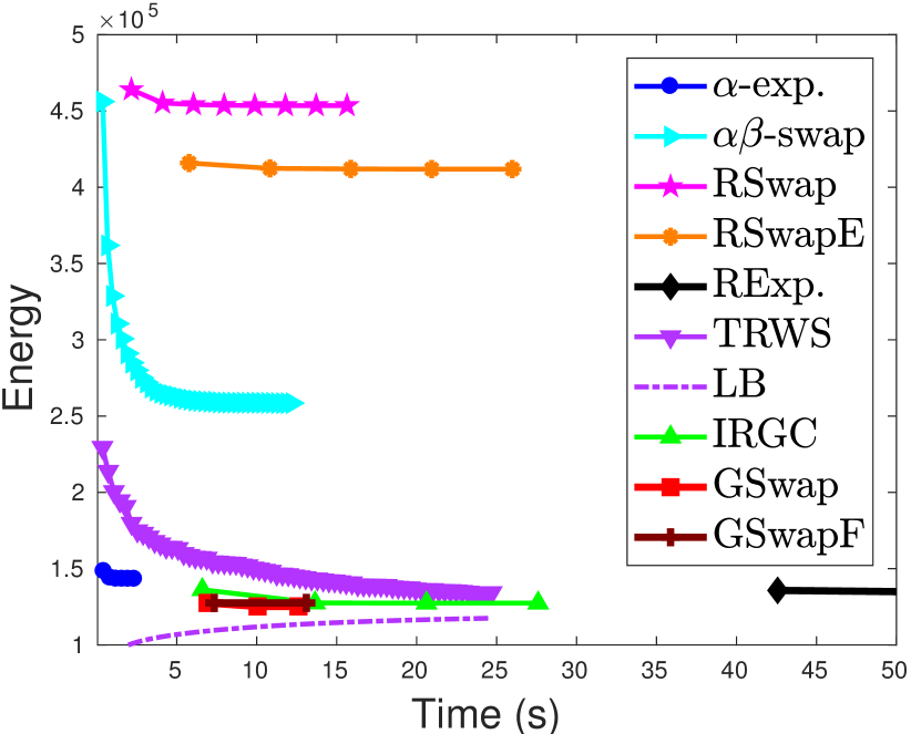
(a) Map, Trunc. quadratic

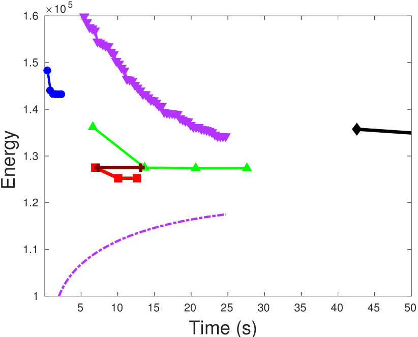
(b) Map, Zoomed-in

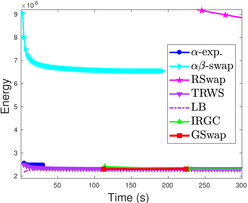
(c) Cones, Cauchy function

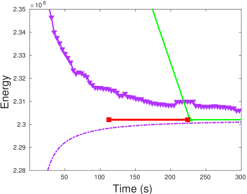
(d) Cones, Zoomed-in

Figure 1: Energy versus time plots for the algorithms for two stereo problems. The plots are zoomed-in to show the finer details. Both versions of our algorithm significantly outperformed both versions of range-swap and obtained the lowest energy faster than the baselines. (best viewed in color)

Results.

The final energies and execution times corresponding to the stereo problems are summarized in Table 1. The energy versus time plots for some representative problems are shown in Fig. 1. Note that in all cases, both versions of our generalized range-move algorithm significantly outperformed both versions of range-swap algorithm, in terms of both energy (up to 3 times lower energy) and running time (up to 24 times faster). This indicates the significance of optimizing over a larger set of active variables and labels at each iteration. Note that among two versions of generalized range-move, GSwapF yielded virtually the same energy as GSwap for the case it is applicable. Furthermore, our method is $2-9$ times faster than the nearest competitor IRGC. Overall, both versions of our algorithm yielded the lowest energy, or an energy that is virtually the same as the lowest one, in shorter time.

5 Conclusion

Both our versions of generalized range-move algorithm, GSwap and GSwapF, substantially outperformed the other move-making algorithms for robust non-convex priors such as truncated quadratic and Cauchy function. The nearest competitor is the Iteratively Reweighted Graph Cut (IRGC) algorithm, which is not a move-making algorithm, and is notably slower in most cases. The superior performance of our generalizations highlights the significance of optimizing over a larger set of active variables and labels at each iteration.

6 Supplementary material

In this section, we first summarize the parameters defining the energy function. Next, we analyze the behaviour of our generalized version of range-move and then we discuss the results with truncated linear pairwise potentials and initialization with $\alpha$-expansion. We would like to point out that the conclusions made in the main paper still hold.

6.1 Energy parameters

As mentioned in the main paper, we employed five instances from the Middlebury dataset [14, 15]: Map, Venus, Sawtooth, Teddy and Cones and one instance from KITTI [7]. For all the problems we used the unary potentials of [3] and used three different pairwise potentials, namely, truncated linear: $g(x)=\min(x,T)$, truncated quadratic: $g(x)=\min(x^{2},T^{2})$, and Cauchy function: $g(x)=T^{2}/2\log(1+(x/T)^{2})$ [8]. The parameters defining the pairwise potentials are summarized in in Table 2.

6.2 Generalized range-move analysis.

We visualize convergence by plotting the generalized Huber energy ($E^{h}$) and the actual truncated convex energy ($E^{g}$) (see Section 2 in the main paper) against the number of iterations. For two stereo problems, this is shown in Fig. 2. Note that the truncated convex energy ($E^{g}$) continues to decrease, whereas the Huber energy ($E^{h}$) increases. This demonstrates that the algorithm is minimizing the desired truncated convex energy, and not the Huber energy. Moreover, the fraction of pixels changed in each iteration (that is, pixels whose labels were updated) is plotted in Fig. 3. Here, both versions of the generalized range-move algorithm rapidly obtained reasonable solutions and then go into a fine-tuning phase where only a small number of pixels are updated at each iteration. However, the number of active variables is close to (or the same as) the number of pixels in the image in both the cases.

Problem	$w_{ij}$	$\ell$	$T$
Map	4	30	6
Venus	50	20	3
Sawtooth	20	20	3
Teddy	$\left\{\begin{array}[]{ll}30&\mbox{if $\nabla_{ij}\leq 10$}\\ 10&\mbox{otherwise}\end{array}\right.$	60	8
Cones	10	60	8
KITTI	20	40	8

Table 2: Pairwise potential $E_{ij}(x_{i},x_{j})=w_{ij}\,g(|x_{i}-x_{j}|)$ used for the stereo problems where $\ell$ denotes the number of labels. Here $g(x)$ is convex if $x\leq T$ and concave otherwise, and $\nabla_{ij}$ denotes the absolute intensity difference between the pixels $i$ and $j$ in the left image.

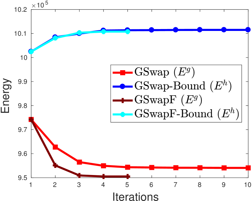
(a) Sawtooth, Trunc. linear

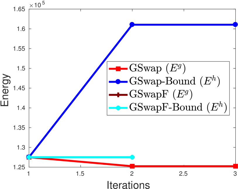
(b) Map, Trunc. quadratic

Figure 2: The generalized Huber energy ($E^{h}$) and the actual truncated convex energy ($E^{g}$) at each iteration, for both versions of our algorithm for two stereo problems. Note that in both the cases, the truncated convex energy continues to decrease, whereas the Huber energy increases. This demonstrates that the algorithms are minimizing the desired truncated convex energy, and not the Huber energy. Furthermore, in Map, while GSwapF was stuck after the first iteration (at the optimal of $E^{h}$), GSwap was able to decrease the energy further. (best viewed in color)

(a) Sawtooth, Trunc. linear

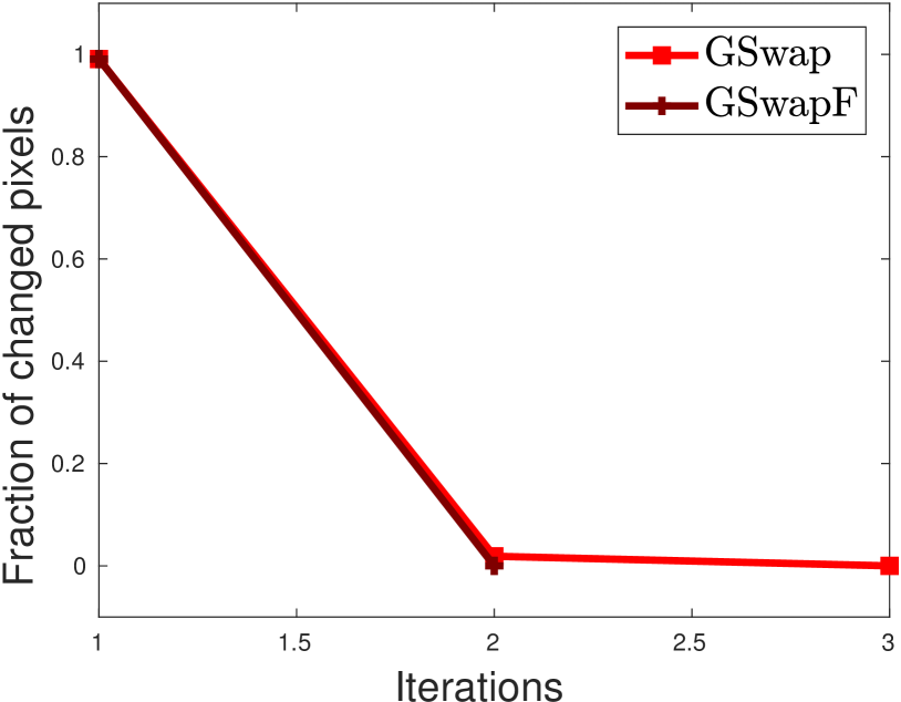
(b) Map, Trunc. quadratic

Figure 3: Fraction of changed pixels at each iteration for both versions of our algorithm and two stereo problems. Note that for both the versions, after the second iteration the fraction of changed pixels is close to zero, which can be interpreted as a fine-tuning phase. (best viewed in color)

6.3 Additional experiments

Truncated linear potentials.

We note that, with truncated linear potentials, $\alpha$-expansion outperforms our generalized range-moves. This is mainly because, truncated linear is a metric (considered easier than non-metric potentials [2, 6]) and $\alpha$-expansion was specifically designed to handle such metric potentials. This evidence is previously observed in [2, 17] and range-moves were shown to outperform $\alpha$-expansion when the pairwise term is "far" from metric, e.g., truncated quadratic or Cauchy prior. This is observed in the main paper as well.

Initialization with $\alpha$-expansion.

Note that range-swap was initialized with $\alpha$-expansion in the original paper [17]. Therefore, for fairer comparison, we initialize range-swap (RSwap) and extended range-swap (RSwapE) with $\alpha$-expansion and compare the results against our algorithm in Table 3. Note the improvement in energies for RSwap and RSwapE with this initialization. This suggests that range-swap is heavily dependent on the initialization. In contrast, we observed that our generalized versions of range-swap algorithm (GSwap, GSwapF), were insensitive to initialization. Similar results are observed for range-expansion, TRWS and IRGC as well.

Even in this case, our generalized versions clearly outperformed both versions of range-swap, but the improvement over range-swap is not significant, which is understandable as range-swap started with a very good initialization.

	Algorithm	Map		Venus		Sawtooth		Teddy		Cones		KITTI
		E[$10^{3}$]	T[s]	E[$10^{3}$]	T[s]	E[$10^{3}$]	T[s]	E[$10^{3}$]	T[s]	E[$10^{3}$]	T[s]	E[$10^{3}$]	T[s]
Trunc. quadratic	RSwap	453.6	16	7958.5	34	2559.5	22	3723.0	2483	6918.3	3689	5503.4	62890
	E+RSwap	132.9	8	3122.4	13	1050.6	10	3074.6	902	2798.2	427	5503.4	20032
	RSwapE	411.9	26	5740.1	113	1660.6	73	3264.3	3397	7289.9	4637	5497.8	116938
	E+RSwapE	130.7	26	3080.6	49	1041.7	36	3047.8	1664	2770.1	952	5497.8	54217
	GSwap	125.2	13	3080.6	13	1042.8	11	2985.3	108	2694.9	93	5492.1	5949
	GSwapF	127.5	13	3080.6	14	1042.8	12	2985.3	119	2694.9	103	5492.1	6621
Cauchy	RSwap	355.0	26	7240.0	105	2430.8	54	3480.9	3728	7108.9	2160	5052.6	79778
	E+RSwap	104.0	10	2612.2	18	853.5	14	2512.9	1081	2346.2	322	4917.7	60156
	GSwap	89.3	13	2558.4	28	843.7	42	2424.4	114	2302.0	224	4820.0	8312

Table 3: Comparison of the minimum energies (E, scaled down by $10^{3}$) and execution times (T) for stereo problems with different robust priors. Here, RSwap and RSwapE are initialized with $\alpha$-expansion, prefixed by ‘E+’. Even in this case, our generalized versions clearly outperformed both versions of range-swap but understandably, the gap is smaller.

References

- [1] T. Ajanthan, R. Hartley, and M. Salzmann. Memory efficient max-flow for multi-label submodular MRFs. CVPR, 2016.
- [2] T. Ajanthan, R. Hartley, M. Salzmann, and H. Li. Iteratively reweighted graph cut for multi-label MRFs with non-convex priors. CVPR, 2015.
- [3] S. Birchfield and C. Tomasi. A pixel dissimilarity measure that is insensitive to image sampling. PAMI, 1998.
- [4] E. Boros and P. L. Hammer. Pseudo-boolean optimization. Discrete applied mathematics, 2002.
- [5] Y. Boykov and V. Kolmogorov. An experimental comparison of min-cut/max-flow algorithms for energy minimization in vision. PAMI, 2004.
- [6] Y. Boykov, O. Veksler, and R. Zabih. Fast approximate energy minimization via graph cuts. PAMI, 2001.
- [7] A. Geiger, P. Lenz, C. Stiller, and R. Urtasun. Vision meets robotics: The KITTI dataset. The International Journal of Robotics Research, 2013.
- [8] R. Hartley and A. Zisserman. Multiple view geometry in computer vision. Cambridge University Press, 2003.
- [9] H. Ishikawa. Exact optimization for Markov random fields with convex priors. PAMI, 2003.
- [10] V. Kolmogorov. Convergent tree-reweighted message passing for energy minimization. PAMI, 2006.
- [11] M. P. Kumar and P. H. Torr. Improved moves for truncated convex models. NIPS, 2009.
- [12] C. Rother, V. Kolmogorov, V. Lempitsky, and M. Szummer. Optimizing binary MRFs via extended roof duality. CVPR, 2007.
- [13] C. Rother, S. Kumar, V. Kolmogorov, and A. Blake. Digital tapestry [automatic image synthesis]. CVPR, 2005.
- [14] D. Scharstein and R. Szeliski. A taxonomy and evaluation of dense two-frame stereo correspondence algorithms. IJCV, 2002.
- [15] D. Scharstein and R. Szeliski. High-accuracy stereo depth maps using structured light. CVPR, 2003.
- [16] D. Schlesinger and B. Flach. Transforming an arbitrary minsum problem into a binary one. TU, Fak. Informatik, 2006.
- [17] O. Veksler. Multi-label moves for MRFs with truncated convex priors. IJCV, 2012.