Massless bosons on domain walls
– Jackiw-Rebbi-like mechanism for bosonic fields –

Abstract

It is important to obtain (nearly) massless localized modes for the low-energy four-dimensional effective field theory in the brane-world scenario. We propose a mechanism for bosonic zero modes using the field-dependent kinetic function in the classical field theory set-up. As a particularly simple case, we consider a domain wall in five dimensions, and show that massless states for scalar (0-form), vector (1-form), and tensor (2-form) fields appear on a domain wall, which may be called topological because of robustness of their existence (insensitive to continuous deformations of parameters). The spin of localized massless bosons is selected by the shape of the nonlinear kinetic function, analogously to the chirality selection of fermion by the well-known Jackiw-Rebbi mechanism. Several explicitly solvable examples are given. We consider not only (anti)BPS domain walls in non-compact extra dimension but also non-BPS domain walls in compact extra dimension.

I Introduction

A long time ago, Jackiw and Rebbi showed that massless fermions are trapped by a topological soliton, namely a domain wall Jackiw:1975fn . As it turns out, this property is robust since it depends on topological aspects of a given theory alone and it is otherwise insensitive to the details. This idea has become ubiquitous within a vast area of modern physics. Let us give several examples. Topological kinks in polyacetylene are described by Su, Schrieffer, and Heeger Su:1979ua , and quantized solitons of the one-dimensional Neel state are studied by Haldane Haldane:1983ru . Rubakov and Shaposhnikov Rubakov:1983bb studied the possibility that our (3+1)-dimensional universe is embedded in higher dimensions, which is an early proposal of the so-called brane-world scenario ArkaniHamed:1998rs ; Antoniadis:1998ig ; Randall:1999ee ; Randall:1999vf . The Jackiw-Rebbi mechanism naturally provides massless chiral fermions (leptons and quarks) on a domain wall (a $3$-brane) in five dimensions. The left- or right-handed chirality is selected by the profile of the domain wall (kink) background solution. The mechanism has also been used to treat chiral fermions in lattice QCD, the so-called domain wall fermion, in Refs. Kaplan:1992bt ; Shamir:1993zy ; Furman:1994ky . Furthermore, there is an intimate connection between the Jackiw-Rebbi mechanism and a topological phase of matter which is one of the highlights in the last decade. There, an interplay between topology and massless edge (surface) modes has revealed new, rich properties of matter Hasan:2010xy ; Qi:2011zya .

These massless modes on edges are all fermionic states. Thus, we are lead to a natural question: Do massless bosons, especially gauge bosons, also robustly appear on domain walls (edges)? In this paper, we answer this question in the affirmative.

We arrived at this question not under the necessity of application to some materials in condensed matter. Rather, we have encountered it in our recent studies on quite different topic, the dynamical construction of brane-world scenario by topological solitons Arai:2012cx ; Arai:2013mwa ; Arai:2017ntb ; Arai:2017lfv ; Arai:2018rwf ; Arai:2018uoy . A necessary condition common to most brane-world models is that all Standard Model particles, except for four-dimensional gravitons, must be localized on the 3-brane. Namely, fermions, scalar and vector bosons must be localized on the 3-brane. It is desirable for a localization mechanism not to depend on details of the model. The Jackiw-Rebbi mechanism is indeed a prime example of such a mechanism, providing chiral fermions on a domain wall (3-brane) Rubakov:1983bb . How about bosons? The Standard Model also has bosonic fields: the Higgs field and $SU(3)\times SU(2)\times U(1)$ gauge bosons. Unlike fermions, however, a robust localization mechanism for bosons, especially non-Abelian Yang-Mills fields, is not widely agreed on. There were many works so far Dvali:2000rx ; Kehagias:2000au ; Dubovsky:2001pe ; Ghoroku:2001zu ; Akhmedov:2001ny ; Kogan:2001wp ; Abe:2002rj ; Laine:2002rh ; Maru:2003mx ; Batell:2006dp ; Guerrero:2009ac ; Cruz:2010zz ; Chumbes:2011zt ; Germani:2011cv ; Delsate:2011aa ; Cruz:2012kd ; Herrera-Aguilar:2014oua ; Zhao:2014gka ; Vaquera-Araujo:2014tia ; Alencar:2014moa ; Alencar:2015awa ; Alencar:2015oka ; Alencar:2015rtc ; Alencar:2017dqb ; Zhao:2017epp . Among them, one of the most popular idea relies on strongly coupled dynamics: a domain wall in confining vacua. A concrete model in four spacetime dimensions was explicitly proposed Dvali:1996xe . Due to the so-called dual Meisner effect, (chromo)electric field cannot invade the bulk, so that massless gauge fields are confined inside the wall. This mechanism is clearly independent of the details. However, since it is based on strong coupling dynamics which is not very well understood in four let alone five dimensions, it is very hard to quantitatively deal with any physics related to massless four-dimensional gauge fields. Therefore, in practice the confinement in higher dimensions was simply assumed to take place, see for example Refs. Libanov:2000uf ; Frere:2000dc ; Frere:2001ug ; Frere:2003yv ; Volkas ; Volkas2 ; Callen:2010mx .

Alternatively, a phenomenological model with a field-dependent kinetic term for gauge fields was considered in six spacetime dimensions ArkaniHamed:1998rs . One does not need to assume confinement in higher dimensions. Rather, it can be thought of as an effective description of confinement in terms of classical fields Kogut:1974sn ; Friedberg:1976eg ; Friedberg:1977xf ; Friedberg:1978sc ; Fukuda:1977wj ; Fukuda:2008mz ; Fukuda:2009zz . Hence, one can quantitatively study phenomena involving the massless four-dimensional gauge fields. A supersymmetric model has been constructed in five spacetime dimensions Ohta:2010fu , and further developments into unified theories beyond the Standard Model followed Arai:2012cx ; Arai:2013mwa ; Arai:2017ntb ; Arai:2017lfv ; Arai:2018rwf ; Arai:2018uoy , see also Okada:2017omx ; Okada:2018von . A detailed study of localization by the field-dependent gauge kinetic terms was done earlier in Dubovsky:2001pe , and another study for nonsupersymmetric model with/without gravity was developed in Chumbes:2011zt , see also a recent review paper Liu:2017gcn .

In this paper, we will reanalyze the localization of massless gauge fields on a domain wall via the field-dependent gauge kinetic term from a different viewpoint where we do not need the speculative connection between it and confinement. Instead, we find a common mathematical structure and a mapping between our localization mechanism of gauge fields and the Jackiw-Rebbi mechanism for fermions. We call this underlying mathematical structure for bosons as Jackiw-Rebbi-like mechanism for bosons. As we will show explicitly, the presence of massless gauge fields on a domain wall relies only on boundary conditions. Thus, it is topological in the sense that it does not depend on precise form of the Lagrangian. Once we recognize the massless gauge fields as topological, we will show that the Jackiw-Rebbi-like mechanism for bosons works not only vector (1-form) fields but also for scalar (0-form) and tensor (2-form) fields. Since there is no obvious reason for massless 0- and 2-form tensor fields to be related to confinement, the Jackiw-Rebbi-like mechanism for bosons is a nice and concrete explanation alternative to the confinment. We will work on domain walls in 5 dimensions in this work. Similarly to the selection of chirality of four-dimensional fermion by the wall, we will show the Jackiw-Rebbi-like mechanism selects the spin of localized massless bosons: It selects between four-dimensional vector or scalar (tensor or vector) in the case of five-dimensional vector (tensor) bosonic fields.

Here, let us make distinctions between this paper and previous works clear. First of all, this work presents a different point of view that the Jackiw-Rebbi-like mechanism plays a main role for the localization. Admittedly, there is a partial overlap between the models we study in Sec. IV.1 and those in Ref. Chumbes:2011zt . However, treatment of extra components of bosonic fields (components perpendicular to the domain wall; $A_{y}$ for vector fields and $\theta_{\mu y}$ for tensor fields) are clearly different. We do not take the axial gauge of $A_{y}=0$ (We will explicitly show that the axial gauge is inadequate to discover massless modes). This is especially important if we consider a pair of a wall and an anti-wall in a compact extra dimension since additional physical massless bosons arise from $A_{y}$ and $\theta_{\mu y}$ as we will show in Sec. V.

The organization of the paper is as follows. We briefly describe well-known facts about domain walls in Sec. II. Topological edge states are explained in Sec. III. In the first subsection we review the Jackiw-Rebbi mechanism for fermions and the rest is devoted for scalar, vector, and tensor bosonic fields. We provide several explicit models in Sec. IV. Only in Sec. V, we consider a pair of a wall and an anti-wall with a compact extra dimension. Phenomenological implications are also discussed.

II Domain walls: A brief review

Let us consider a scalar model in non-compact flat five-dimensional spacetime ($D=5$)

$${\cal L}_{\rm DW}=\partial_{M}T\partial^{M}T-W_{T}^{2}\,,\quad(M=0,1,2,3,4)\,,$$ (1)

where we have expressed, for later convenience, a scalar potential $V(T)=W_{T}(T)^{2}$ in terms of a “superpotential” $W(T)$ which is an arbitrary function of a real scalar field $T$. Hereafter we use the notation such as

$$W_{T}=\frac{dW}{dT},\qquad W_{TT}=\frac{d^{2}W}{dT^{2}}.$$ (2)

We assume that there exist multiple discrete vacua satisfying $W_{T}=0$. Let $T=T(y)$ be a domain wall solution which interpolates adjacent vacua at $y=\pm\infty$ ($y$ stands for one of the spatial coordinates). The static equation of motion reads

$$-T^{\prime\prime}+W_{T}W_{TT}=0\,,$$ (3)

where the prime denotes a derivative in terms of $y$. Let us investigate the mass spectrum by perturbing $T$ about the background domain wall solution as $T(y)\to T(y)+\tau(x^{\mu},y)$ with $\tau$ being a small fluctuation of the scalar field. The linearized equation of motion is found as

$$\left(\square-\partial_{y}^{2}+W_{TT}^{2}+W_{T}W_{TTT}\right)\tau=0,$$ (4)

where $W_{T},W_{TT}$, and $W_{TTT}$ should be understood as those evaluated at the domain wall solution $T=T(y)$. Hence, the mass spectrum is determined by solving the eigenvalue problem in one dimension with the $n$-th eigenfunction $g_{n}$ corresponding to the mass squared eigenvalue $m_{n}^{2}$

$$\left(-\partial_{y}^{2}+W_{TT}^{2}+W_{T}W_{TTT}\right)g_{n}=m_{n}^{2}g_{n}.$$ (5)

Irrespective of the details of the superpotential $W$, there always exists a normalizable zero mode. To see this, let us differentiate Eq. (3) once by $y$

$$\left(-\partial_{y}^{2}+W_{TT}^{2}+W_{T}W_{TTT}\right)T^{\prime}=0.$$ (6)

Thus, we find a solution with zero eigenvalue (apart from the normalization constant)

$$g_{0}=T^{\prime}.$$ (7)

The presence of this normalizable zero mode is robust, because it is nothing but the Nambu-Goldstone zero mode associated with the spontaneously broken translational symmetry.

Stability of the domain wall background is ensured by topology. When a static configuration $T$ is a function of $y$, we can derive the well-known Bogomol’nyi completion form for the energy density ${\cal E}$ as

$${\cal E}=T^{\prime}{}^{2}+W_{T}^{2}=\left(T^{\prime}\mp W_{T}\right)^{2}\pm 2T^{\prime}W_{T}\geq\pm 2W^{\prime}\,.$$ (8)

This Bogomol’nyi inequality is useful by choosing the upper (lower) sign for $W^{\prime}>0$ ($W^{\prime}<0$). It is saturated by solutions of the so-called BPS equation

$$T^{\prime}=\pm W_{T}.$$ (9)

We call the upper sign the BPS while the lower sign the antiBPS. Tension of the domain wall is finite since we have assumed a boundary condition with $T^{\prime}=\pm W_{T}\to 0$ as $|y|\to\infty$. It is straightforward to verify that any solution of the BPS equation solves the full EOM (3). Tension of the BPS domain wall reads

$$\sigma=\int^{\infty}_{-\infty}dy\,{\cal E}=2\left|W\left(T(+\infty)\right)-W\left(T(-\infty)\right)\right|.$$ (10)

This is a topological quantity. To see this, let us define a conserved current by

$$j^{\alpha}=\epsilon^{\alpha\beta}\partial_{\beta}W(T),\qquad(\alpha,\beta=0,y).$$ (11)

Then the topological charge $q$ reads

$$q=\int^{\infty}_{-\infty}dy\,j^{0}=\int^{\infty}_{-\infty}dy\,\partial_{y}W(T)=W\left(T(+\infty)\right)-W\left(T(-\infty)\right).$$ (12)

After appropriately normalized, we find that the (anti)BPS domain wall has the topological charge $(-)1$.

If the background configuration is a BPS or an antiBPS solution rather than a general solution of field equation in Eq. (3), we can obtain more precise informations as follows. Using the BPS equation $T^{\prime}=W_{T}$, the eigenvalue equation (5) can be rewritten as

$$\text{BPS}: Q^{\dagger}Qg_{n}=m_{n}^{2}g_{n}\,,$$ (13)

where we have introduced 1st order differential operators

$$Q=-\partial_{y}+W_{TT}(T(y)),\qquad Q^{\dagger}=\partial_{y}+W_{TT}(T(y)).$$ (14)

Similarly, for the antiBPS solution ($T^{\prime}=-W_{T}$), the eigenvalue equation can be rewritten as

$$\text{antiBPS}: QQ^{\dagger}g_{n}=m_{n}^{2}g_{n}\,.$$ (15)

The Hamiltonians $Q^{\dagger}Q$ and $QQ^{\dagger}$ are semi-positive definite, so there are no tachyonic instabilities. It is interesting to note that the above system of equations constitutes a supersymmetric quantum mechanics Witten:1981nf (SQM). The SQM superpotential ${\cal X}(y)$ is defined as

$$Q=-\partial_{y}+{\cal X}^{\prime}.$$ (16)

In this case of scalar field $T$ for the BPS domain wall, the SQM superpotential ${\cal X}$ is related to the “superpotential” $W$ in the $D=5$ field theory Lagrangian (1) as

$${\cal X}(y)\big{|}_{\rm(anti)BPS}=\pm\frac{1}{2}\log W_{T}(T(y))^{2}\,.$$ (17)

By using the (anti)BPS equation, the translational zero mode $g_{0}$ can be expressed as

$$g_{0}(y)\big{|}_{\rm(anti)BPS}=W_{T}(T(y)).$$ (18)

We emphasize that the SQM form is valid for the translational zero mode only if the domain wall satisfies the BPS equation.

III Massless states on domain walls

III.1 Domain wall fermions: A review on the Jackiw-Rebbi mechanism

In addition to scalar fields in ${\cal L}_{\rm DW}$, let us consider a five-dimensional Dirac fermion $\Psi$ in the form

$${\cal L}_{\rm F}=i\bar{\Psi}\Gamma^{M}\partial_{M}\Psi-{\cal M}(T)\bar{\Psi}\Psi\,.$$ (19)

The gamma matrices in $D=5$ are related to those in $D=4$ by $\Gamma^{\mu}=\gamma^{\mu}$ and $\Gamma^{4}=i\gamma_{5}$. The field-dependent “mass” ${\cal M}(T)$ is just a coupling function of scalar fields multiplying the term quadratic in fermion fields. It becomes a $5D$ fermion mass only when it is a constant and independent of any fields. We assume that the function ${\cal M}(T)$ is real. When considering the Kaluza-Klein decomposition to (infinitely many) $4D$ components, there is no reason for massless $4D$ fermions to exist with a generic ${\cal M}(T)$, except for the well-known Jackiw-Rebbi mechanism Jackiw:1975fn . The mechanism ensures the existence of massless fermions localized on a domain wall, and works in both even and odd dimensions. The masslessness of the fermion resulting from the Jackiw-Rebbi mechanism is stable against small deformations of parameters. In this sense, the Jackiw-Rebbi fermion is topological.

To see how the Jackiw-Rebbi mechanism works, let us investigate mass spectra of the fermion around the domain wall background $T(y)$. We assume that asymptotic values of ${\cal M}(T(y=\pm\infty))$ at left and right infinity are non zero and have opposite sign, as in the typical kink-like configuration, see Fig. 1.

$${\cal M}(T(y=-\infty))\times{\cal M}(T(y=+\infty))<0.$$ (20)

Linearized equations of motion for fermionic fluctuations $\Psi$ (using the same character $\Psi$ for the small fluctuation) reads

$$i\gamma^{\mu}\partial_{\mu}\Psi-\gamma_{5}\partial_{y}\Psi-{\cal M}\Psi=0\,.$$ (21)

Let us define a “Hamiltonian”

$$H_{5}=-\gamma_{5}\partial_{y}-{\cal M}\,.$$ (22)

A normalizable zero eigenstate of $H_{5}\left|0\right>=0$ can be easily found by multiplying $\gamma_{5}$ from left and considering eigenstates of $\gamma_{5}\left|\pm\right>=\pm\left|\pm\right>$ for which it holds

$${\cal Q}\left|-\right>=0\,,\qquad{\cal Q}^{\dagger}\left|+\right>=0\,,$$ (23)

where the ${\cal Q}$ and ${\cal Q}^{\dagger}$ operators are defined by

$${\cal Q}=-\partial_{y}+{\cal M}(y)\,,\qquad{\cal Q}^{\dagger}=\partial_{y}+{\cal M}(y)\,.$$ (24)

In the coordinate representation these states reads

$$\left<y|-\right>\equiv f_{0}(y)=e^{\int^{y}d\lambda\,{\cal M}(T(\lambda))}\,,\qquad\left<y|+\right>\equiv\tilde{f}_{0}(y)=e^{-\int^{y}d\lambda\,{\cal M}(T(\lambda))}\,,$$ (25)

up to normalization constants. Since the domain wall connects different vacua with opposite sign for ${\cal M}(T(y=-\infty))$ and ${\cal M}(T(y=+\infty))$ as in Eq. (20), ${\cal M}(T(y))$ must vanish at a finite value of $y$, usually around the center of the domain wall. When ${\cal M}(T(y))$ increasingly (decreasingly) goes across zero, the right(left)-handed fermion is localized on the domain wall, see Fig. 1. This property does not depend on any details of the solution, and it is the heart of the Jackiw-Rebbi model Jackiw:1975fn . In terms of a modern terminology, the massless fermion is often called the topological edge state Hasan:2010xy .

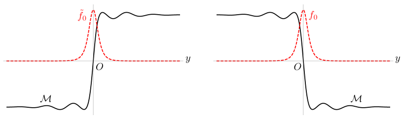
Figure 1: The field-dependent “mass” ${\cal M}(T(y))$ and the associated topological edge states (fermion zero modes). The solid curves are ${\cal M}=\pm\left(\tanh y+\frac{1}{10}e^{-y^{2}/100}\sin y\right)$, and the broken red curves correspond to the mode functions of the fermion zero modes.

As was mentioned in the footnote 2, these fermions should be interpreted as four dimensional fermionic particles confined inside the domain wall.

Let us make our statement clearer. Hereafter, we use the Jackiw-Rebbi mechanism for fermions for the following meaning. When the field dependent “mass” ${\cal M}(T)$ defined in Eq. (19) satisfies the condition (20), either left- or right-handed massless fermion appears around a point where ${\cal M}$ vanishes. The chirality of the massless fermion is determined by the sign of the asymptotic value ${\cal M}(y=+\infty)$ : Left-handed for ${\cal M}(y=+\infty)<0$, and right-handed for ${\cal M}(y=+\infty)>0$. We also define topological particles as those massless particles that remain massless under continuous deformations of parameters, and are not explained by symmetry reasons such as a spontaneously broken rigid symmetry. The domain wall fermion is a typical topological particle which does not disappear against any continuous changes without violating the condition given in Eq. (20).

For later uses, let us give a complete analysis for the mass spectra. Firstly, we decompose $\Psi$ into $\Psi_{L}$ and $\Psi_{R}$ which are the eigenstates of $\gamma_{5}$ as $\gamma_{5}\Psi_{L}=-\Psi_{L}$ and $\gamma_{5}\Psi_{R}=\Psi_{R}$. We find

$$i\gamma^{\mu}\partial_{\mu}\Psi_{R}={\cal Q}\Psi_{L},\qquad i\gamma^{\mu}\partial_{\mu}\Psi_{L}={\cal Q}^{\dagger}\Psi_{R}\,.$$ (26)

Eliminating $\Psi_{R}$ ($\Psi_{L}$), we reach the following equations

$$\left(\square+{\cal Q}^{\dagger}{\cal Q}\right)\Psi_{L}=0,\quad\left(\square+{\cal Q}{\cal Q}^{\dagger}\right)\Psi_{R}=0.$$ (27)

Thus, the physical spectra for $\Psi_{L,R}$ are determined by solving the 1D eigenvalue problems

$${\cal Q}^{\dagger}{\cal Q}f_{n}=M_{n}^{2}f_{n},\qquad{\cal Q}{\cal Q}^{\dagger}\tilde{f}_{n}=M_{n}^{2}\tilde{f}_{n}.$$ (28)

We again encounter a 1D SQM problem with the superpotential ${\cal Q}=-\partial_{y}+{\cal Y}^{\prime}(y)$ given in (24),

$${\cal Y}(y)=\int^{y}d\lambda\ {\cal M}(T(\lambda)).$$ (29)

We would like to emphasize that this formula is correct regardless of whether the background solution is (anti)BPS or non-BPS. This is in contrast to the fluctuation of $T$ field given in Eq. (13) or (15) which are valid only for the (anti)BPS background solution. As before, the 1D Hamiltonians are semi-positive definite, so that there are no tachyonic modes. Furthermore, due to the SQM structure, $\Psi_{L}$ and $\Psi_{R}$ share the identical mass spectra except for possible zero modes, in accord with the fact that any modes with a nonvanishing mass consist of both chiralities in even dimensions.

We will now turn to massless bosons in subsequent sections.

III.2 Domain wall scalars

Contrary to fermions, the protection mechanism for masslessness of scalar fields is not known except for the symmetry reason associated with the spontaneously broken rigid symmetry with a continuous parameter, namely the Nambu-Goldstone boson. For example, we found in Sec. II a normalizable scalar zero mode on the domain wall background, whose existence is ensured by the spontaneously broken translational symmetry.

Guided by the Jackiw-Rebbi mechanism for fermions, one might be tempted to try considering a real scalar field $\Phi$ whose coupling function for quadratic term is given by the same field-dependent “mass” ${\cal M}(T)$ as in Eq. (19):

$${\cal L}_{\rm S}=\frac{1}{2}\partial_{M}\Phi\partial^{M}\Phi-\frac{1}{2}{\cal M}(T)^{2}\Phi^{2},$$ (30)

in addition to the Lagrangians (1). Since ${\cal M}(T)^{2}\Phi^{2}$ is semi-positive definite, $\Phi$ remains inert as $\Phi=0$, when $T$ takes the domain wall configuration as a solution of the equation of motion. Since the 1D eigenvalue problem for the fluctuation of $\Phi$ on this background has a positive definite potential, ${\cal M}(T(y))^{2}$, it is obvious that there are only massive modes. This illustrates that the naive attempt does not work for bosons.

We now wish to propose a mechanism for a domain wall scalar boson, namely a model with a massless scalar mode whose existence is insensitive to change of parameters. Instead of tuning a scalar potential, we turn to use a nonlinear kinetic term with a field-dependent kinetic function. Let us assume the following simple Lagrangian in addition to ${\cal L}_{\rm DW}$:

$${\cal L}_{0}=\beta(T)^{2}\partial_{M}\Phi\partial^{M}\Phi.$$ (31)

A field-dependent “coupling” $\beta(T)$ is a function of the scalar field $T$ multiplying the term quadratic in $\partial_{M}\Phi$. This form is inspired by nonlinear kinetic function for gauge and form fields, which are described in subsequent sections. One can characterize absence of a potential for $\Phi$ as a result of a “shift” symmetry $\Phi\to\Phi+{\rm constant}$. We do not consider a mixed term like $g(T)\partial_{M}T\partial^{M}\Phi$ in this paper, since adding it is a large deformation in the sense that it changes the structure of Lagrangian qualitatively. Alternatively, one can forbid it by imposing the parity $\Phi\to-\Phi$.

Vacuum condition is $\Phi=\text{const.}$ and $W_{T}=0$. As before, we assume that there are several discrete vacua. Then, $T$ has a nontrivial domain wall configuration whereas $\Phi=\text{const.}$ as a background solution. As for the mass spectra of fluctuations on the background domain wall solution, the linearized equation for the $T$ field is unchanged from Eq. (4). Therefore, a normalizable translational zero mode always exists with the mode function $T^{\prime}(y)$ and the massless effective field $\tau_{0}(x^{\mu})$ in 4D, i.e. $\tau(x^{\mu},y)=T^{\prime}(y)\tau_{0}(x^{\mu})$.

In the rest of this subsection, we will study mass spectra of the scalar field $\Phi$. The linearized equation for small fluctuation $\Phi$ is given by (we will use the same notation $\Phi$ for the fluctuation):

$$\partial_{M}\left(\beta(T)^{2}\partial^{M}\Phi\right)=0.$$ (32)

First of all, we introduce a canonically normalized field $\varphi$

$$\Phi=\frac{\varphi}{\sqrt{2}\beta}.$$ (33)

This nonlinear field redefinition transforms Eq. (32) into

$$\left(\square+D^{\dagger}D\right)\varphi=0,$$ (34)

where we defined

$$D=-\partial_{y}+{\cal Z}^{\prime}(y),\qquad D^{\dagger}=\partial_{y}+{\cal Z}^{\prime}(y),$$ (35)

with a 1D SQM superpotential

$${\cal Z}(y)=\frac{1}{2}\int^{y}d\lambda\,\frac{d}{d\lambda}\log\beta(T(\lambda))^{2}=\frac{1}{2}\log\beta(T(y))^{2}.$$ (36)

Note that this is valid for any background solutions since we have not used the (anti)BPS equation. Thus, we have obtained another 1D eigenvalue problem with the SQM structure

$$D^{\dagger}Dh_{n}=\mu_{n}^{2}h_{n},$$ (37)

Unlike the fermionic case, the super partner $DD^{\dagger}$ is absent in the problem.

The solution with zero eigenvalue is unique and is given by

$$h_{0}(y)=e^{\int^{y}d\lambda\,{\cal Z}^{\prime}(\lambda)}=e^{{\cal Z}(y)}=\beta(T(y)).$$ (38)

This is a normalizable physical state whenever $\beta(T(y))$ is square integrable. We will call the massless scalar boson topological only in the limited sense that it is stable against small changes of parameters in the nonlinear kinetic function $\beta$. As is clear from the derivation, it is not the NG boson for the spontaneously broken rigid symmetry such as translation. We observe that the 1D eigenvalue problem for mass spectra of scalar field becomes identical to that of fermion by identifying the function ${\cal Z}^{\prime}(y)=d\log\beta(T(y))/dy$ in the operator $D$ with ${\cal Y}^{\prime}(y)={\cal M}(T(y))$ in the operator ${\cal Q}$

$${\cal Y}^{\prime}(y)={\cal M}(T(y))\quad\leftrightarrow\quad{\cal Z}^{\prime}(y)=\frac{d\log\beta(T(y))}{dy}.$$ (39)

We assume that the function ${\cal Z}^{\prime}(y)$ goes across zero as ${\cal M}(y)$ in Fig. 1. Namely, the function ${\cal Z}^{\prime}(y)$ satisfies the following condition as in the fermion case in Eq. (20)

$${\cal Z}^{\prime}(y=-\infty)\times{\cal Z}^{\prime}(y=+\infty)<0.$$ (40)

In the present case of scalar field, we have to choose ${\cal Z}^{\prime}(y=+\infty)<0$ for $h_{0}$ to be normalizable.​ In the opposite case with ${\cal Z}^{\prime}(y=+\infty)>0$, there are no normalizable massless modes.

We now come to a highlight of this work. We define the Jackiw-Rebbi-like mechanism for bosons as follows: When the field-dependent “coupling” $\beta(T)$ defined in Eq. (31) satisfies the condition (40), a localized massless scalar boson appears and is localized around a point where $d\beta(T(y))/dy$ vanishes. Similarly to the fermion case, the massless boson is stable against any continuous changes which do not violate the condition (40) for $\beta^{\prime}/\beta$. In short, the massless scalar field in Eq. (38) is a topological edge state which is supported by the Jackiw-Rebbi-like mechanism for bosons.

III.3 Domain wall vectors/scalars

In this section we consider (1-form) gauge fields. We consider a gauge invariant Lagrangian similar to ${\cal L}_{0}$ in Eq. (31),

$${\cal L}_{1}=-\beta(T)^{2}{\cal F}_{MN}{\cal F}^{MN}.$$ (41)

Here, we only consider an Abelian gauge field ${\cal A}_{M}$ with the field strength ${\cal F}_{MN}=\partial_{M}{\cal A}_{N}-\partial_{N}{\cal A}_{M}$ just for simplicity, but it is straightforward to extend the following results to Yang-Mills fields Arai:2018rwf .

As was explained in the Introduction, the Lagrangian (41) is a model for the localized gauge fields on domain walls in the brane-world-scenario. To localize gauge fields on topological defects like domain walls, it was recognized that the confining phase is needed in the bulk, and a toy model in four spacetime dimensions was explicitly proposed Dvali:1996xe . The field-dependent kinetic term for gauge fields was considered together with further explicit toy model in six spacetime dimensions ArkaniHamed:1998rs , and an explicit model has been constructed in five spacetime dimensions Ohta:2010fu . Another study for nonsupersymmetric model with/without gravity was developed in Chumbes:2011zt . The coefficient $\beta$ in Eq. (41) can be considered as an inverse of the position dependent gauge coupling after the scalar field $T$ takes a nontrivial $y$-dependent values as the background. Bulk with $\beta=0$ implies infinitely large gauge coupling, which is a semiclassical realization of the confining vacuum Kogut:1974sn ; Friedberg:1976eg ; Friedberg:1977xf ; Friedberg:1978sc ; Fukuda:1977wj ; Fukuda:2008mz ; Fukuda:2009zz . Due to the so-called dual Meisner effect, (chromo)electric field cannot invade the bulk, so that massless gauge fields are confined inside a finite region (for us it is inside the domain wall) where $\beta$ is not zero.

Leaving aside the above qualitative interpretation of the model based on a somewhat speculative intuition of confinement in dimensions higher than four, we will now focus on the underlying mathematical structure of the localization mechanism inherent in the model (41). It is very close to the model of topological massless scalar fields in Sec. III.2. Namely, the massless gauge field is supported by the Jackiw-Rebbi-like mechanism for bosons. In order to see the relation clearly, let us investigate the mass spectrum of the gauge field about the domain wall background $T(y)$. Firstly, we need to fix unphysical gauge degree of freedom. The most popular gauge choice is the axial gauge ${\cal A}_{y}=0$, see for example Refs. Ohta:2010fu ; Chumbes:2011zt . However, one should be careful to deal with a possible normalizable zero mode in ${\cal A}_{y}$, since, if it exists, it is gauge invariant and cannot be gauged away. Therefore, one cannot fully remove ${\cal A}_{y}(x,y)$ before confirming the absence of normalizable zero modes. To clarify this point, we have developed a new gauge fixing condition recently by adding the following gauge fixing term Okada:2017omx ; Arai:2018uoy ; Okada:2018von

$${\cal L}_{\rm GF}=-\frac{2}{\xi}\beta(T)^{2}\left[\partial_{\mu}{\cal A}^{\mu}-\frac{\xi}{\beta(T)^{2}}\partial_{y}\left(\beta(T)^{2}{\cal A}_{y}\right)\right]^{2},$$ (42)

where $\xi$ is an arbitrary gauge fixing parameter. We call this the extended $R_{\xi}$ gauge Arai:2018uoy .

To study the mass spectra, let us consider small fluctuations $A_{M}$ around the domain wall background and we define a canonically normalized fields in five spacetime dimensions, which will make the analogy to the Jackiw-Rebbi mechanism most explicit

$${\cal A}_{M}=\frac{A_{M}}{2\beta(T)}.$$ (43)

Then the linearized equations of motion in the generalized $R_{\xi}$ gauge are given by Arai:2018uoy :

$$\left[\eta^{\mu\nu}\square-\left(1-\frac{1}{\xi}\right)\partial^{\mu}\partial^{\nu}+\eta^{\mu\nu}D^{\dagger}D\right]A_{\nu}=0,$$ (44)

$$\left(\square+\xi DD^{\dagger}\right)A_{y}=0.$$ (45)

We again encounter $D$ and $D^{\dagger}$ defined in Eq. (35). However, not only $D^{\dagger}D$ but also $DD^{\dagger}$ comes into play, unlike the case of the scalar field. Thus, the 1D eigenvalue problem for mass spectra exhibits the 1D SQM structure in precise analogy with the Jackiw-Rebbi mechanism for fermions

$$D^{\dagger}Dh_{n}=\mu_{n}^{2}h_{n},\qquad DD^{\dagger}\tilde{h}_{n}=\mu_{n}^{2}\tilde{h}_{n}.$$ (46)

As before, the eigenvalue spectra of $D^{\dagger}D$ and $DD^{\dagger}$ coincide except for zero eigenvalue. We observe that the massive modes of $A_{y}$ are unphysical, since their masses depend on the gauge-fixing parameter $\xi$, and will be cancelled by the ghost fields with the same mass. However, $n=0$ is special. Eq. (45) shows that the zero mode $A_{y}^{(n=0)}$ of $A_{y}$ is just a massless scalar field. The gauge fixing parameter $\xi$ disappears from Eq. (45), so that $A_{y}$ of $n=0$ is not a gauge-dependent degree of freedom. The observation that the normalizable zero mode of $A_{y}$ can be physical scalar field is missed in many previous works using ${\cal A}_{y}=0$ gauge. For the zero mode $n=0$ of $A_{\mu}$, Eq. (44) reduces to the linearized equation for the massless photon in the usual covariant gauge.

The mode functions with the zero eigenvalue are explicitly given by

$$h_{0}(y)=\beta(T(y)),\qquad\tilde{h}_{0}(y)=\frac{1}{\beta(T(y))}\,.$$ (47)

Thus, as in the scalar case, the physical massless gauge field appears on the domain wall whenever $\beta(T(y))$ is square integrable. This is the case when the condition Eq. (40) is satisfied with ${\cal Z}^{\prime}(y=+\infty)<0$. On the other hand, $\tilde{h}_{0}(y)$ is not normalizable, as long as we consider noncompact space $-\infty<y<\infty$. Hence $A_{y}$ does not supply a physical massless scalar field. Up to this point, the final result turns out to be the same as that obtained in the axial gauge ${\cal A}_{y}=0$. However, there are two other possibilities.

The first possibility is that the condition in Eq. (40) is satisfied with ${\cal Z}^{\prime}(y=+\infty)>0$. Then the physical massless field localized on the domain wall is scalar, since $\beta(T(y))^{-1}$ is square integrable. In this case, the massless vector field becomes unphysical because it is no longer normalizable. Thus, the spin of massless bosons is determined by the sign of the asymptotic value of the function ${\cal Z}^{\prime}(y=+\infty)$ : The massless boson is vector if ${\cal Z}^{\prime}(y=+\infty)<0$ or is scalar if ${\cal Z}^{\prime}(y=+\infty)>0$, similarly to the selection of chirality in the case of the Jackiw-Rebbi mechanism for fermions.

Another possibility is to consider compact space such as the circle for the extra dimension $y$. We will discuss this possibility in Sec. V.

III.4 Domain wall tensors/vectors

Let us now consider a two-form field in five dimensions with the Lagrangian

$${\cal L}_{2}=\beta(T)^{2}{\cal H}_{MNL}{\cal H}^{MNL}.$$ (48)

Here, we consider a two-form field $\theta_{MN}=-\theta_{NM}$ with a field strength ${\cal H}_{MNL}=\partial_{M}\theta_{NL}+\partial_{L}\theta_{MN}+\partial_{N}\theta_{LM}$. The above Lagrangian is invariant under the gauge transformation $\theta_{MN}\to\theta_{MN}+\partial_{M}\Lambda_{N}-\partial_{N}\Lambda_{M}$, where $\Lambda_{M}$ is an arbitrary $U(1)$ gauge field. To fix the gauge and clarify unphysical degrees of freedom, we choose to add the following gauge-fixing terms

$${\cal L}_{\rm GF}=\frac{6}{\xi}\beta(T)^{2}\left(\partial_{\mu}\theta^{\mu\nu}+\frac{\xi}{\beta(T)^{2}}\partial_{y}\bigl{(}\beta(T)^{2}\theta_{\phantom{\nu}y}^{\nu}\bigr{)}\right)^{2}-\frac{6}{\eta}\beta(T)^{2}\bigl{(}\partial_{\mu}\theta_{\phantom{\mu}y}^{\mu}\bigr{)}^{2}.$$ (49)

Similarly to the generalized $R_{\xi}$ gauge employed in the previous section, these terms are devised in such a way as to eliminate the mixing terms between extra-dimensional and four-dimensional components. Notice that we have two independent gauge-fixing parameters, namely $\xi$ and $\eta$.

Let us investigate mass spectra of fluctuation fields of $\theta_{MN}$ around the domain wall background. In terms of the canonically normalized fields

$$\theta_{\mu\nu}=\frac{h_{\mu\nu}}{\beta(T)},\hskip 14.22636pt\theta_{\mu y}=\frac{B_{\mu}}{\sqrt{12}\,\beta(T)}$$ (50)

the linearized equations of motion read

$$\Bigl{[}\eta^{\mu\rho}\eta^{\nu\sigma}\square+\eta^{\mu\sigma}\partial^{\rho}\partial^{\nu}+\eta^{\nu\rho}\partial^{\sigma}\partial^{\mu}+\tfrac{2}{\xi}\eta^{\nu\sigma}\partial^{\mu}\partial^{\rho}+\eta^{\mu\rho}\eta^{\nu\sigma}D^{\dagger}D\Bigr{]}h_{\rho\sigma}=0,$$ (51)

$$\Bigl{[}\eta^{\mu\nu}\square-\bigl{(}1-\tfrac{1}{\eta}\bigr{)}\partial^{\mu}\partial^{\nu}+\xi\eta^{\mu\nu}DD^{\dagger}\Bigr{]}B_{\nu}=0.$$ (52)

Thus, no new 1D eigenvalue problems arise as the differential operators $D$ and $D^{\dagger}$ are the same as for scalar (zero-form) and vector (one-form) fields.

Similarly to the vector fields, existence of physical massless modes is guaranteed by the condition in Eq. (40). Namely, the spin of the physical massless bosons is determined by the sign of the asymptotic value of the function ${\cal Z}^{\prime}(y=+\infty)$ : Only the tensor field $\theta_{\mu\nu}$ has a zero mode if ${\cal Z}^{\prime}(y=+\infty)<0$ since $\beta(T(y))$ is square integrable, whereas only the vector field $\theta_{\mu y}$ has a zero mode if ${\cal Z}^{\prime}(y=+\infty)>0$ since $\beta^{-1}(T(y))$ is square integrable.

Let us consider the case of ${\cal Z}^{\prime}(y=+\infty)<0$, where we have the massless mode $h_{\mu\nu}^{(0)}$. From the four-dimensional point of view of effective field theory, the massless mode can be understood as a scalar field via a duality,

$$\partial_{\mu}h_{\nu\rho}^{(0)}+\partial_{\rho}h_{\mu\nu}^{(0)}+\partial_{\nu}h_{\rho\mu}^{(0)}=\varepsilon_{\mu\nu\rho\sigma}\partial^{\sigma}\phi\,,$$ (53)

where $\phi$ is a massless scalar. On the other hand, the massive states $h_{\mu\nu}^{(n)}$ can be interpreted as massive vector fields, whereas all the massive states in the second tower $B_{\mu}^{(n)}$ are unphysical as their masses are proportional to $\xi$.

In contrast, if ${\cal Z}^{\prime}(y=+\infty)>0$, the normalizable zero mode $B_{\mu}^{(0)}$ now exists. It is easy to see that $B_{\mu}^{(0)}$ acts as a gauge field under $y$-independent gauge transformations of $\theta_{MN}$ and, therefore, there is a localized $U(1)$ gauge field in the spectrum.

In the case of ${\cal Z}^{\prime}(y=+\infty)<0$ ($\beta$ being square integrable), the spectrum of localized particles for two-form field is a massless dual scalar $\phi$ and a tower of massive vector fields dual to $h_{\mu\nu}^{(n\neq 0)}$. This spectrum is identical to the spectrum for one-form field ($A_{y}^{(0)}$ and $A_{\mu}^{(n\neq 0)}$) in the case of ${\cal Z}^{\prime}(y=+\infty)>0$ ($1/\beta$ being square integrable), as shown in the previous section.

Similarly, if ${\cal Z}^{\prime}(y=+\infty)>0$ for two-form field, we have the spectrum of a massless gauge field $B_{\mu}^{(0)}$ and a tower of massive vector fields dual to $h_{\mu\nu}^{(n\neq 0)}$, which precisely coincides with the spectrum ($A_{\mu}^{(0)}$ and $A_{\mu}^{(n\neq 0)}$) for one-form in the case of ${\cal Z}^{\prime}(y=+\infty)<0$.

This correspondence can be easily understood via on-shell duality between two-forms and one-forms in five dimensions. Indeed, if we look at the full equation of motion

$$\partial_{M}\left(\beta^{2}{\cal H}^{MNL}\right)=0\,,$$ (54)

we can solve it by setting

$${\cal H}_{MNL}=\beta^{-2}\bigl{(}\varepsilon_{MNLPQ}{\cal F}^{PQ}\bigr{)}\,,$$ (55)

where ${\cal F}^{PQ}=\partial^{P}{\cal A}^{Q}-\partial^{Q}{\cal A}^{P}$ and ${\cal A}_{M}$ is some gauge field. Note that the Bianchi identity

$$\varepsilon^{MNLPQ}\partial_{N}{\cal H}_{LPQ}=0$$ (56)

translates into the equation of motion for the gauge field, i.e. $\partial_{M}\bigl{(}\beta^{-2}{\cal F}^{MN}\bigr{)}=0$ which is the same equation of motion as in the previous section but it comes with $\beta^{-2}$ in place of $\beta^{2}$.

IV Simple models

IV.1 A class of calculable models

As we have stressed so far, there are no strong constraints for both ${\cal M}(T)$ and $\beta(T)$. However, it is extremely convenient to choose a particular form in order to gain a calculability even in the case of non-BPS background solution. One of the simplest example we choose is

$${\cal M}(T)=\epsilon_{\rm F}W_{TT}(T),\qquad\beta(T)=W_{T}(T)^{\epsilon_{\rm B}}\,,$$ (57)

where $\epsilon_{\rm B,F}$ is either $+1$ or $-1$. With the choice of ${\cal M}(T)$, ${\cal L}_{\rm DW}+{\cal L}_{\rm F}$ is close to the Wess-Zumino SUSY model in $D=4$. However, it is not our intention to stick to genuine supersymmetric models in five spacetime dimensions. Instead, we only use the model to gain calculability hoping to get general qualitative features in a simple and transparent manner without being constrained by supersymmetry.

In the rest of this section, we will focus on the BPS domain wall which satisfies $T^{\prime}=W_{T}(T)$. The case of antiBPS domain wall is straightforward, and nonBPS cases will be studied in Sec. V. The translational NG boson is given in Eq. (18).

The normalizable fermionic zero mode given in Eq. (25) reads

$$f_{0}(y)\big{|}_{\rm BPS} = e^{\epsilon_{\rm F}\int^{y}d\lambda\,W_{TT}(T(\lambda))}=W_{T}(T(y))^{\epsilon_{\rm F}},$$ (58)

$$\tilde{f}_{0}(y)\big{|}_{\rm BPS} = e^{-\epsilon_{\rm F}\int^{y}d\lambda\,W_{TT}(T(\lambda))}=W_{T}(T(y))^{-\epsilon_{\rm F}},$$ (59)

where we have used the BPS equation. Thus, when $\epsilon_{\rm F}=+1(-1)$, the left-handed (right-handed) massless fermion appears on the domain wall. Interestingly, the normalizable mode functions for the NG boson (18) coincides with that of the topological fermion. This is due to the SUSY-like structure in ${\cal L}_{\rm DW}+{\cal L}_{\rm F}$. Namely, the normalizable bosonic and fermionic zero mode can be regarded as “supersymmetric” partners.

The bosonic solutions with zero eigenvalue in Eq. (47) for the choice of $\beta$ in Eq. (57) read

$$h_{0}(y)\big{|}_{\rm BPS}=W_{T}(T(y))^{\epsilon_{\rm B}},\qquad\tilde{h}_{0}(y)\big{|}_{\rm BPS}=W_{T}(T(y))^{-\epsilon_{\rm B}},$$ (60)

where we have not used the BPS equation. Thus, when $\epsilon_{\rm B}=+1$, there exist a massless scalar $\Phi$, vector $A_{\mu}$, and a tensor $\theta_{\mu\nu}$ gauge field on the domain wall for ${\cal L}_{0,1,2,}$, respectively. On the other hand, when $\epsilon_{\rm B}=-1$, no normalizable zero modes exist for ${\cal L}_{0}$, and a scalar $A_{y}$ and vector $\theta_{\mu y}$ massless modes appears for ${\cal L}_{1,2}$, respectively. Although there is no obvious hint of supersymmetry between the nonlinear kinetic function in Lagrangians ${\cal L}_{0,1,2,}$ and ${\cal L}_{\rm DW}$ or ${\cal L}_{\rm F}$, the mode function of the topological bosons turn out to coincide with those of the translational NG boson and the topological massless fermion. The only link that one can find is the SQM structure common to all these fields in the case of the BPS background solution. The mass spectra coincide not only for the massless mode but also for all the massive Kaluza-Klein states, since the 1D SQM superpotentials which determine the mass spectra are common to all fields for the BPS domain wall, i.e.

$${\cal X}(y)\big{|}_{\rm BPS}={\cal Y}(y)\big{|}_{\rm BPS}={\cal Z}(y)\big{|}_{\rm BPS}=\frac{1}{2}\log W_{T}(T(y))^{2}.$$ (61)

IV.2 Sine-Gordon domain wall

The simplest example is the sine-Gordon model with the superpotential

$$W(T)=\frac{\Lambda^{3}}{g^{2}}\sin\frac{g}{\Lambda}T.$$ (62)

The BPS domain wall solutions satisfying $T^{\prime}=W_{T}$ are given by

$$T(y)=\frac{\Lambda}{g}\left(2\arctan e^{\Lambda y}-\frac{\pi}{2}+2n\pi\right)\to\left\{\begin{array}[]{ccc}\left(-\frac{\pi}{2}+2n\pi\right)\frac{\Lambda}{g}&&y\to-\infty\\ \left(\frac{\pi}{2}+2n\pi\right)\frac{\Lambda}{g}&&y\to\infty\end{array}\right.\,.$$ (65)

For these solutions, we have

$$W_{T}(T(y))=\frac{\Lambda^{2}}{g}{\rm sech}\,\Lambda y,\qquad W_{TT}(T(y))=-\Lambda\tanh\Lambda y.$$ (66)

There are another set of the BPS solutions given by

$$T(y)=\frac{\Lambda}{g}\left(2\arctan e^{-\Lambda y}+\frac{\pi}{2}+2n\pi\right)\to\left\{\begin{array}[]{ccc}\left(\frac{3\pi}{2}+2n\pi\right)\frac{\Lambda}{g}&&y\to-\infty\\ \left(\frac{\pi}{2}+2n\pi\right)\frac{\Lambda}{g}&&y\to\infty\end{array}\right.\,.$$ (69)

For these solutions, we have

$$W_{T}(T(y))=-\frac{\Lambda^{2}}{g}{\rm sech}\,\Lambda y,\qquad W_{TT}(T(y))=-\Lambda\tanh\Lambda y.$$ (70)

The fact that $W_{TT}(T(y))$ goes across 0 once ensures presence of the topological massless states.

Since the background is BPS, all the 1D SQM superpotentials agree. Therefore, the mass spectra are determined only by $W_{TT}$ in the operator $Q=-\partial_{y}+W_{TT}(T(y))$. The corresponding SQM Hamiltonians for both BPS solutions are given by

$$Q^{\dagger}Q=-\partial_{y}^{2}+\Lambda^{2}\left(2\tanh^{2}\Lambda y-1\right),\qquad QQ^{\dagger}=-\partial_{y}^{2}+\Lambda^{2}.$$ (71)

We have ${\cal Q}^{\dagger}{\cal Q}=Q^{\dagger}Q$ and ${\cal Q}{\cal Q}^{\dagger}=QQ^{\dagger}$ for $\epsilon_{\rm F}=+1$, while ${\cal Q}^{\dagger}{\cal Q}=QQ^{\dagger}$ and ${\cal Q}{\cal Q}^{\dagger}=Q^{\dagger}Q$ for $\epsilon_{\rm F}=-1$. Similarly, we also have $D^{\dagger}D=Q^{\dagger}Q$ and $DD^{\dagger}=QQ^{\dagger}$ for $\epsilon_{\rm B}=+1$, while $D^{\dagger}D=QQ^{\dagger}$ and $DD^{\dagger}=Q^{\dagger}Q$ for $\epsilon_{\rm B}=-1$. Therefore, there exist a unique discrete bound state, which is nothing but the normalizable zero mode for $\epsilon_{\rm F}=\epsilon_{\rm B}=+1$,

$$g_{0}=f_{0}=h_{0}\propto W_{T}\propto{\rm sech}\Lambda y.$$ (72)

For the other choice of $\epsilon_{\rm F,B}$, one should replace $f_{0}$ ($h_{0}$) by $\tilde{f}_{0}$ ($\tilde{h}_{0}$). There are no other discrete states both in the $Q^{\dagger}Q$ and $QQ^{\dagger}$ sectors. All the massive modes are continuum states (scattering in the bulk) given as

$$f_{k} = Q^{\dagger}e^{iky}=\left(ik-\Lambda\tanh\Lambda y\right)e^{iky},$$ (73)

$$\tilde{f}_{k} = e^{iky},$$ (74)

with the mass square

$$m(k)^{2}=k^{2}+\Lambda^{2}.$$ (75)

IV.3 $T^{4}$ domain wall

Our second example is the $T^{4}$ domain wall in the model with cubic super potential

$$W(T)=\frac{\Lambda^{2}}{g}T-\frac{g}{3}T^{3}.$$ (76)

The BPS domain wall solution is given by

$$T(y)=\frac{\Lambda}{g}\tanh\Lambda y.$$ (77)

For this background, we have

$$W_{T}(T(y))=\frac{\Lambda^{2}}{g}{\rm sech}^{2}\Lambda y,\qquad W_{TT}(T(y))=-2\Lambda\tanh\Lambda y.$$ (78)

The factor 2 appears compared to the sine-Gordon model. The factor 2 corresponds to the number of the localized modes as we will see below.

As before, it is enough to investigate ${\cal Q}^{\dagger}{\cal Q}$ and ${\cal Q}{\cal Q}^{\dagger}$ because the background is BPS. We have

$${\cal Q}^{\dagger}{\cal Q}=-\partial_{y}^{2}+2\Lambda^{2}\left(3\tanh^{2}\Lambda y-1\right),\qquad{\cal Q}{\cal Q}^{\dagger}=-\partial_{y}^{2}+2\Lambda^{2}\left(\tanh^{2}\Lambda y+1\right).$$ (79)

There is unique normalizable zero mode in the ${\cal Q}^{\dagger}{\cal Q}$ sector

$$f_{0}\propto W_{T}\propto{\rm sech}^{2}\Lambda y.$$ (80)

Also there exist a massive discrete state

$$f_{1} \propto {\cal Q}^{\dagger}{\rm sech}\Lambda\propto\tanh\Lambda y~{}{\rm sech}\Lambda y,$$ (81)

$$\tilde{f}_{1} \propto {\rm sech}\Lambda y.$$ (82)

All the other states are continuum states (scattering in the bulk).

V Non-BPS domain walls in compact extra dimension

V.1 Quasi solvable example

So far, we have only considered models with flat non-compact extra dimension. In this section we will study physical spectra about the domain walls in compact extra dimension. For simplicity, we consider the extra dimension to be $S^{1}$ with a radius $R$. Unlike the non compact case, all the mode functions are, of course, normalizable if they are regular. Since the profile function $T(y)$ should be periodic, the background solution has to be non-BPS which includes both BPS and antiBPS domain walls.

To be concrete, let us again consider the sine-Gordon model with the superpotential given in Eq. (62). A non-BPS solution with multiple domain walls is known Maru:2001gf as

$$T(y)=\frac{\Lambda}{g}{\rm am}\left(\frac{\Lambda}{k}y,k\right),$$ (83)

where ${\rm am}(x,k)$ denotes the Jacobi amplitude function with a real parameter $k$. Since $T$ can be regarded as an angular variable with periodicity $2\pi\Lambda/g$, we can identify the compactification radius $R$ as

$$2\pi R=\frac{4k\,K(k)}{\Lambda},$$ (84)

where $K(k)$ is the complete elliptic integral of the first kind. The solution has BPS and antiBPS domain walls alternatively sitting at anti-podal points of $S^{1}$. Namely, the BPS domain wall sits at the origin $y=0$ whereas the antiBPS domain wall sits at $y=\pi R$. The background solutions with $k<1$ and $k>1$ are qualitatively quite different ($k=1$ corresponds to either BPS or antiBPS), see Fig. 2. $|gT/\Lambda|$ never goes across $\pi/2$ for the $k>1$ case, whereas it monotonically increases (decreases) for the $k<1$ case.

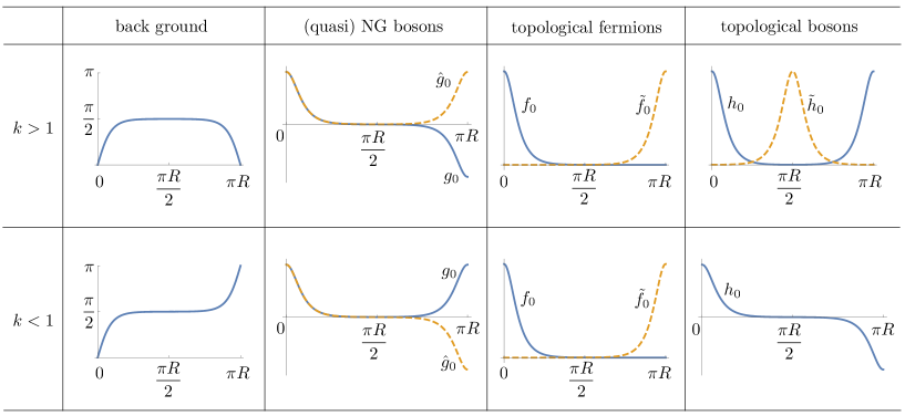
Figure 2: Non-BPS domain wall solutions with the BPS and antiBPS walls at $y=0$ and $\pi R$ in the sine-Gordon model. The left-most column shows the background configuration $gT/\Lambda$, and the other three columns show mode functions of the small fluctuations for the case of $\epsilon_{\rm F,B}=+1$. In the figures, only the half period is shown. The case of $\epsilon_{\rm F,B}=-1$ can be obtained by exchanging $(f_{0},h_{0})$ by $(\tilde{f}_{0},\tilde{h}_{0})$.

Since the above solution is non-BPS, the (anti)BPS equation $T^{\prime}=\pm W_{T}$ is not satisfied. Therefore, mass spectra of the translational NG bosons, the topological fermions, and the topological bosons split. Let us start with the fluctuation of $T$. Several light modes are explicitly known as

$$g_{0} \propto {\rm dn}\left(\frac{\Lambda y}{k},k\right),\quad m_{0}^{2}=0,$$ (85)

$$\hat{g}_{0} \propto {\rm cn}\left(\frac{\Lambda y}{k},k\right),\quad\hat{m}_{0}^{2}=\frac{1-k^{2}}{k^{2}}\Lambda^{2},$$ (86)

$$g_{2} \propto {\rm sn}\left(\frac{\Lambda y}{k},k\right),\quad m_{2}^{2}=\frac{\Lambda^{2}}{k^{2}}.$$ (87)

Note that $g_{0}=T^{\prime}$ is a genuine translational Nambu-Goldstone mode which is exactly massless. On the other hand, $\hat{g}_{0}$ is quasi Nambu-Goldstone mode which corresponds to the relative distance (so-called radion). It is tachyonic for $k>1$ while it is massive for $k<1$. The reason why the quasi zero mode is lifted is that unlike for $g_{0}$ there is no symmetric reasoning for relative distance moduli. One can also say that the lifting proves that the translational zero modes (genuine translational NG and relative distance moduli) are not topologically protected. If they were topological, both $g_{0}$ and $\hat{g}_{0}$ would have remained as massless. These mode functions are depicted in the 2nd column from the left of Fig. 2.

Next, let us see the fermions. We chose the coupling function ${\cal M}(T)$ for fermions as

$${\cal M}(T)=\epsilon_{\rm F}W_{TT}(T).$$ (88)

Then, normalizable zero modes can be explicitly found as

$$f_{0} \propto e^{\epsilon_{\rm F}\int^{y}d\lambda\,W_{TT}(T(\lambda))}=\left[{\rm dn}\left(\frac{\Lambda y}{k},k\right)-k\,{\rm cn}\left(\frac{\Lambda y}{k},k\right)\right]^{-\epsilon_{\rm F}},$$ (89)

$$\tilde{f}_{0} \propto e^{-\epsilon_{\rm F}\int^{y}d\lambda\,W_{TT}(T(\lambda))}=\left[{\rm dn}\left(\frac{\Lambda y}{k},k\right)-k\,{\rm cn}\left(\frac{\Lambda y}{k},k\right)\right]^{\epsilon_{\rm F}}.$$ (90)

As is well known, $f_{0}$ is localized around the BPS domain wall at $y=0$ while $\tilde{f}_{0}$ is around the antiBPS domain wall at $y=\pi R$ for $\epsilon_{\rm F}=+1$, see the third column from left of Fig. 2. (The mode functions of zero modes are exchanged for $\epsilon_{\rm F}=-1$.) They are normalizable since the extra dimension is compact. Note that unlike the translational NG bosons, both $f_{0}$ and $\tilde{f}_{0}$ remain as genuine massless modes since they are topological.

Finally, let us see the gauge bosons for the case

$$\beta(T)=W_{T}(T)^{\epsilon_{\rm B}}.$$ (91)

We find the exact normalizable zero modes for the topological bosons as

$$h_{0} \propto \beta=W_{T}^{\epsilon_{\rm B}}={\rm cn}\left(\frac{\Lambda y}{k},k\right)^{\epsilon_{\rm B}},$$ (92)

$$\tilde{h}_{0} \propto \beta^{-1}=W_{T}^{-\epsilon_{\rm B}}={\rm cn}\left(\frac{\Lambda y}{k},k\right)^{-\epsilon_{\rm B}}.$$ (93)

When $k>1$, ${\rm cn}(x,k)$ never goes across 0. Therefore, both $h_{0}$ and $\tilde{h}_{0}$ are normalizable. The mode function $h_{0}$ for the zero mode of $A_{\mu}$ is localized at the domain walls at $y=0$ and $\pi R$ while $\tilde{h}_{0}$ for $A_{y}$ is localized between them when $\epsilon_{\rm B}=+1$. If $\epsilon_{\rm B}=-1$, the localized positions of $h_{0}$ and $\tilde{h}_{0}$ are exchanged. When $k<1$, ${\rm cn}(x,k)$ goes across 0. Therefore $\tilde{h}_{0}$ ($h_{0}$) is singular and non-normalizable for $\epsilon_{\rm B}=+1$ ($\epsilon_{\rm B}=-1$). We show $h_{0}$ and $\tilde{h}_{0}$ for $\epsilon_{\rm B}=+1$ in the right-most column of Fig. 2.

V.2 Phenomenological implications

As is shown in Fig. 2, the localization positions of the topological fermions and topological bosons are sharply different. Interestingly, $h_{0}$ ($\tilde{h}_{0}$) for $\epsilon_{\rm B}=+1$ ($\epsilon_{\rm B}=-1$) have non-zero support around both the BPS and antiBPS domain walls. This leads to several interesting consequences. Before going to explain this, however, one should be careful about the mode functions: $h_{0}$ and $\tilde{h}_{0}$ are the mode functions of the redefined fields $\varphi$, $A_{\mu}$, $A_{y}$, $h_{\mu\nu}$ and $B_{\mu}$. The mode functions for the original fields $\Phi$, ${\cal A}_{M}$ and $\theta_{MN}$ are those divided by $\beta$, see Fig. 3.

$$h_{0}\to\frac{h_{0}}{2\beta}=\text{const.}\,,\qquad\tilde{h}_{0}\to\frac{\tilde{h}_{0}}{2\beta}\propto\beta^{-2}=W_{T}^{-2\epsilon_{\rm B}}\,.$$ (94)

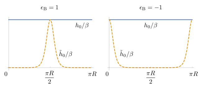
Figure 3: The mode functions of the topological bosons for the non-canonical fields $\Phi,{\cal A}_{M},\theta_{MN}$ around the non-BPS domain wall solution. The case of $\epsilon_{B}=1(-1)$ is shown in the left (right) panel.

In the following, we choose the background solution with $k>1$ which is not afflicted by the problem like non-normalizability of mode functions. For phenomenology in the brane-world scenario, let us concentrate on the (1-form) gauge field in the following. Suppose that the fermion is charged under the $U(1)$ gauge symmetry with unit charge. The covariant derivative is given by ${\cal D}_{M}\Psi=\left(\partial_{M}+i{\cal A}_{M}\right)\Psi$. We find the gauge interactions of massless fermions as

$$\int dy\,\bar{\Psi}\Gamma^{\mu}{\cal D}_{\mu}\Psi \ni \int dy\biggl{(}f_{0}^{2}\bar{\psi}_{L}^{(0)}\gamma^{\mu}\left(\partial_{\mu}+i\frac{h_{0}}{2\beta}A_{\mu}^{(0)}\right)\psi_{L}^{(0)}+\tilde{f}_{0}^{2}\bar{\psi}_{R}^{(0)}\gamma^{\mu}\left(\partial_{\mu}+i\frac{h_{0}}{2\beta}A_{\mu}^{(0)}\right)\psi_{R}^{(0)}\biggr{)}$$ (95)

$$= \bar{\psi}_{L}^{(0)}\gamma^{\mu}\left(\partial_{\mu}+ie_{4}A_{\mu}^{(0)}\right)\psi_{L}^{(0)}+\bar{\psi}_{R}^{(0)}\gamma^{\mu}\left(\partial_{\mu}+ie_{4}A_{\mu}^{(0)}\right)\psi_{R}^{(0)},$$

where we have used the fact that $h_{0}$ is proportional to $\beta$ as $h_{0}=2e_{4}\beta$ with

$$e_{4}^{-2}=4\int_{0}^{2\pi R}dy\,\beta^{2}.$$ (96)

It is important to notice that the effective gauge coupling $e_{4}$ is universal. It is also independent of the fermion mode functions. Hence, the low energy effective theory is a vector-like gauge theory such as QED or QCD in which the left and right handed fermions are coupled with the gauge field with the same strength. In order to have a chiral gauge theory like the Standard Model in our framework, we have to consider the infinitely separated limit $R=\infty$ ($k=1$). This situation is in accord with the usual notion of domain wall fermion in lattice gauge theories.

In contrast to the gauge interactions in four-dimensions, we have an interesting non-universality for the coupling of massless scalar coming from $A_{y}$. The induced Yukawa-type coupling of the scalar $A_{y}^{(0)}$ is given as

$$\int dy\,\bar{\Psi}\Gamma^{y}{\cal D}_{y}\Psi \ni -g_{L}A_{y}^{(0)}\bar{\psi}_{L}^{(0)}\gamma_{5}\psi_{L}^{(0)}-g_{R}A_{y}^{(0)}\bar{\psi}_{R}^{(0)}\gamma_{5}\psi_{R}^{(0)}\,.$$ (97)

where we used the fact that $\tilde{h}_{0}=2\tilde{e}_{4}\beta^{-1}$ as

$$\tilde{e}_{4}^{-2}=4\int_{0}^{2\pi R}dy\,\beta^{-2}.$$ (98)

and defined

$$g_{L} \equiv \int^{2\pi R}_{0}dy\,f_{0}^{2}\frac{\tilde{h}_{0}}{2\beta}=\int_{0}^{2\pi R}dy\,\frac{\tilde{e}_{4}f_{0}^{2}}{\beta^{2}},$$ (99)

$$g_{R} \equiv \int^{2\pi R}_{0}dy\,\tilde{f}_{0}^{2}\frac{\tilde{h}_{0}}{2\beta}=\int_{0}^{2\pi R}dy\,\frac{\tilde{e}_{4}\tilde{f}_{0}^{2}}{\beta^{2}}.$$ (100)

Now, we find that $g_{L(R)}$ plays a role of effective Yukawa coupling for scalar field $A_{y}^{(0)}$. Firstly, since $f_{0}$ ($\tilde{f}_{0}$) and $\tilde{h}_{0}$ are separately localized at different positions as shown in Figs. 2,3 for $\epsilon_{\rm B}=1$, the overlap integrals for $g_{L(R)}$ are exponentially small. This can help to explain smallness of the Yukawa couplings for the first and second generation of quarks and leptons ArkaniHamed:1999dc . Secondly, the scalar field $A_{y}^{(0)}$ can play a role of the Higgs field Hosotani:1983xw ; Hosotani:1983vn . If $A_{y}^{(0)}$ enjoys a non-zero vacuum expectation value (VEV), it immediately means the fermions get masses. Since the Higgs field is originated as the extra-dimensional gauge field, it is natural to expect that quadratic divergences are suppressed thanks to the gauge symmetry in the original five-dimensional Lagrangian as advocated by the gauge-Higgs unification scenario Hatanaka:1998yp . In order to verify if $A_{y}^{(0)}$ actually gets non-zero VEV, one must examine an effective potential due to quantum corrections such as fermion loop correction. We hope to report it in a separate work.

The results in this section are obtained by using a very special simplified model in order to be able to compute mode functions and other quantities in a closed form. However, we wish to stress that all the qualitative features should be valid even if we choose more general functions for the coupling functions such as ${\cal M}(T)$ and $\beta(T)$. We only need to use a numerical method to obtain various quantities in the general setting.

VI Concluding remarks

Fermionic topological edge (surface) states are well known in a vast area of modern physics from high energy physics to condensed matter physics. These fermionic topological states on domain walls are robust and are ensured by the Jackiw-Rebbi mechanism Jackiw:1975fn . In this paper, we showed that bosonic topological edge states also appear on the domain wall by a quite similar mechanism which we call the Jackiw-Rebbi-like mechanism for bosons. We explicitly showed that it universally works for scalar (0-form), vector (1-form), and tensor (2-form) bosonic fields. They are topological, since their presence only relies on boundary condition. For localization of vector fields, it has been argued that confinement phenomenon is necessary Dvali:1996bg ; ArkaniHamed:1998rs ; Ohta:2010fu . But it is difficult to show the confinement mechanism especially in higher-dimensional field theory. On the contrary, the result of this work offers another explanation related to topology. One of the advantages is that it can be applied not only for vector but also scalar and antisymmetric tensor fields, and we can be sure that it works in any spacetime dimensions.

An interesting feature of the Jackiw-Rebbi(-like) mechanism is that for fermions, the domain wall in five dimensions selects four-dimensional chirality. On the other hand, for four-dimensional bosons it selects spin. For vector (tensor) fields, it selects between four-dimensional vector or scalar (tensor or vector). This can only be seen with the appropriate gauge-fixing terms in Eqs. (42) and (49).

We also gave explicit models in Sec. IV which are useful to see general qualitative features in a simple and transparent manner. Furthermore, we studied massless particles around the non-BPS background with a pair of a wall and anti-wall in compact extra dimension in Sec. V. There, we manifestly showed that the translational zero modes, topological fermionic edge modes, and topological bosonic edge modes have all different mode functions as is shown in Fig. 2. We also pointed out possible phenomenological uses of our results. The universality of gauge charges is automatically satisfied, large hierarchy problem of fermion masses of the Standard Model would naturally be resolved, and $A_{y}$ would play a role of the Higgs field as in usual gauge Higgs unification models.

There are several interesting directions for further studies. In this paper we restricted ourselves in five spacetime dimensions just for ease of presentation. If we go to higher dimensions than five, higher antisymmetric tensor (form) fields can appear. We should examine how the selection rules by the domain wall is generalized. We can also consider other solitons like vortex and monopole whose co-dimensions are higher than one. As is the case of domain wall, localization of topological fermions are well known. We will study whether it is true for bosons or not. On the other hand, it is also very interesting to go to lower dimensions. If our bosonic topological states are found in a real material, it is an indirect proof of localization of all the Standard Model particles on a domain wall. Apart from the brane-world perspective, it might be interesting for revealing new properties of topological matters. The domain wall fermions are known to be important in lattice QCD, so we also wonder if the topological localization mechanism of bosons plays some role for improving computer simulations of lattice QCD.

References

- (1) R. Jackiw and C. Rebbi, “Solitons with Fermion Number 1/2,” Phys. Rev. D 13, 3398 (1976). doi:10.1103/PhysRevD.13.3398
- (2) W. P. Su, J. R. Schrieffer and A. J. Heeger, “Solitons in polyacetylene,” Phys. Rev. Lett. 42, 1698 (1979). doi:10.1103/PhysRevLett.42.1698
- (3) F. D. M. Haldane, “Nonlinear field theory of large spin Heisenberg antiferromagnets. Semiclassically quantized solitons of the one-dimensional easy Axis Neel state,” Phys. Rev. Lett. 50, 1153 (1983). doi:10.1103/PhysRevLett.50.1153
- (4) V. A. Rubakov and M. E. Shaposhnikov, “Do We Live Inside a Domain Wall?,” Phys. Lett. 125B, 136 (1983). doi:10.1016/0370-2693(83)91253-4
- (5) N. Arkani-Hamed, S. Dimopoulos and G. R. Dvali, “The Hierarchy problem and new dimensions at a millimeter,” Phys. Lett. B 429, 263 (1998) doi:10.1016/S0370-2693(98)00466-3 [hep-ph/9803315].
- (6) I. Antoniadis, N. Arkani-Hamed, S. Dimopoulos and G. R. Dvali, “New dimensions at a millimeter to a Fermi and superstrings at a TeV,” Phys. Lett. B 436, 257 (1998) doi:10.1016/S0370-2693(98)00860-0 [hep-ph/9804398].
- (7) L. Randall and R. Sundrum, “A Large mass hierarchy from a small extra dimension,” Phys. Rev. Lett. 83, 3370 (1999) doi:10.1103/PhysRevLett.83.3370 [hep-ph/9905221].
- (8) L. Randall and R. Sundrum, “An Alternative to compactification,” Phys. Rev. Lett. 83, 4690 (1999) doi:10.1103/PhysRevLett.83.4690 [hep-th/9906064].
- (9) D. B. Kaplan, “A Method for simulating chiral fermions on the lattice,” Phys. Lett. B 288, 342 (1992) doi:10.1016/0370-2693(92)91112-M [hep-lat/9206013].
- (10) Y. Shamir, “Chiral fermions from lattice boundaries,” Nucl. Phys. B 406, 90 (1993) doi:10.1016/0550-3213(93)90162-I [hep-lat/9303005].
- (11) V. Furman and Y. Shamir, “Axial symmetries in lattice QCD with Kaplan fermions,” Nucl. Phys. B 439, 54 (1995) doi:10.1016/0550-3213(95)00031-M [hep-lat/9405004].
- (12) M. Z. Hasan and C. L. Kane, “Topological Insulators,” Rev. Mod. Phys. 82, 3045 (2010) doi:10.1103/RevModPhys.82.3045 [arXiv:1002.3895 [cond-mat.mes-hall]].
- (13) X. L. Qi and S. C. Zhang, “Topological insulators and superconductors,” Rev. Mod. Phys. 83, no. 4, 1057 (2011) doi:10.1103/RevModPhys.83.1057 [arXiv:1008.2026 [cond-mat.mes-hall]].
- (14) M. Arai, F. Blaschke, M. Eto and N. Sakai, “Matter Fields and Non-Abelian Gauge Fields Localized on Walls,” PTEP 2013, 013B05 (2013) doi:10.1093/ptep/pts050 [arXiv:1208.6219 [hep-th]].
- (15) M. Arai, F. Blaschke, M. Eto and N. Sakai, “Stabilizing matter and gauge fields localized on walls,” PTEP 2013, no. 9, 093B01 (2013) doi:10.1093/ptep/ptt064 [arXiv:1303.5212 [hep-th]].
- (16) M. Arai, F. Blaschke, M. Eto and N. Sakai, “Non-Abelian Gauge Field Localization on Walls and Geometric Higgs Mechanism,” PTEP 2017, no. 5, 053B01 (2017) doi:10.1093/ptep/ptx047 [arXiv:1703.00427 [hep-th]].
- (17) M. Arai, F. Blaschke, M. Eto and N. Sakai, “Grand Unified Brane World Scenario,” Phys. Rev. D 96, no. 11, 115033 (2017) doi:10.1103/PhysRevD.96.115033 [arXiv:1703.00351 [hep-th]].
- (18) M. Arai, F. Blaschke, M. Eto and N. Sakai, “Localized non-Abelian gauge fields in non-compact extra-dimensions,” arXiv:1801.02498 [hep-th].
- (19) M. Arai, F. Blaschke, M. Eto and N. Sakai, “Localization of the Standard Model via the Higgs mechanism and a finite electroweak monopole from non-compact five dimensions,” PTEP 2018, no. 8, 083B04 (2018) doi:10.1093/ptep/pty083 [arXiv:1802.06649 [hep-ph]].
- (20) G. R. Dvali, G. Gabadadze and M. A. Shifman, “(Quasi)localized gauge field on a brane: Dissipating cosmic radiation to extra dimensions?,” Phys. Lett. B 497, 271 (2001) doi:10.1016/S0370-2693(00)01329-0 [hep-th/0010071].
- (21) A. Kehagias and K. Tamvakis, “Localized gravitons, gauge bosons and chiral fermions in smooth spaces generated by a bounce,” Phys. Lett. B 504, 38 (2001) doi:10.1016/S0370-2693(01)00274-X [hep-th/0010112].
- (22) S. L. Dubovsky and V. A. Rubakov, “On models of gauge field localization on a brane,” Int. J. Mod. Phys. A 16, 4331 (2001) doi:10.1142/S0217751X01005286 [hep-th/0105243].
- (23) K. Ghoroku and A. Nakamura, “Massive vector trapping as a gauge boson on a brane,” Phys. Rev. D 65, 084017 (2002) doi:10.1103/PhysRevD.65.084017 [hep-th/0106145].
- (24) E. K. Akhmedov, “Dynamical localization of gauge fields on a brane,” Phys. Lett. B 521, 79 (2001) doi:10.1016/S0370-2693(01)01176-5 [hep-th/0107223].
- (25) I. I. Kogan, S. Mouslopoulos, A. Papazoglou and G. G. Ross, “Multilocalization in multibrane worlds,” Nucl. Phys. B 615, 191 (2001) doi:10.1016/S0550-3213(01)00424-2 [hep-ph/0107307].
- (26) H. Abe, T. Kobayashi, N. Maru and K. Yoshioka, “Field localization in warped gauge theories,” Phys. Rev. D 67, 045019 (2003) doi:10.1103/PhysRevD.67.045019 [hep-ph/0205344].
- (27) M. Laine, H. B. Meyer, K. Rummukainen and M. Shaposhnikov, “Localization and mass generation for nonAbelian gauge fields,” JHEP 0301, 068 (2003) doi:10.1088/1126-6708/2003/01/068 [hep-ph/0211149].
- (28) N. Maru and N. Sakai, “Localized gauge multiplet on a wall,” Prog. Theor. Phys. 111, 907 (2004) doi:10.1143/PTP.111.907 [hep-th/0305222].
- (29) B. Batell and T. Gherghetta, “Yang-Mills Localization in Warped Space,” Phys. Rev. D 75, 025022 (2007) doi:10.1103/PhysRevD.75.025022 [hep-th/0611305].
- (30) R. Guerrero, A. Melfo, N. Pantoja and R. O. Rodriguez, “Gauge field localization on brane worlds,” Phys. Rev. D 81, 086004 (2010) doi:10.1103/PhysRevD.81.086004 [arXiv:0912.0463 [hep-th]].
- (31) W. T. Cruz, M. O. Tahim and C. A. S. Almeida, “Gauge field localization on a dilatonic deformed brane,” Phys. Lett. B 686, 259 (2010). doi:10.1016/j.physletb.2010.02.064
- (32) A. E. R. Chumbes, J. M. Hoff da Silva and M. B. Hott, “A model to localize gauge and tensor fields on thick branes,” Phys. Rev. D 85, 085003 (2012) doi:10.1103/PhysRevD.85.085003 [arXiv:1108.3821 [hep-th]].
- (33) C. Germani, “Spontaneous localization on a brane via a gravitational mechanism,” Phys. Rev. D 85, 055025 (2012) doi:10.1103/PhysRevD.85.055025 [arXiv:1109.3718 [hep-ph]].
- (34) T. Delsate and N. Sawado, “Localizing modes of massive fermions and a U(1) gauge field in the inflating baby-skyrmion branes,” Phys. Rev. D 85, 065025 (2012) doi:10.1103/PhysRevD.85.065025 [arXiv:1112.2714 [gr-qc]].
- (35) W. T. Cruz, A. R. P. Lima and C. A. S. Almeida, Phys. Rev. D 87, no. 4, 045018 (2013) doi:10.1103/PhysRevD.87.045018 [arXiv:1211.7355 [hep-th]].
- (36) A. Herrera-Aguilar, A. D. Rojas and E. Santos-Rodriguez, “Localization of gauge fields in a tachyonic de Sitter thick braneworld,” Eur. Phys. J. C 74, no. 4, 2770 (2014) doi:10.1140/epjc/s10052-014-2770-1 [arXiv:1401.0999 [hep-th]].
- (37) Z. H. Zhao, Y. X. Liu and Y. Zhong, “U(1) gauge field localization on a Bloch brane with Chumbes-Holf da Silva-Hott mechanism,” Phys. Rev. D 90, no. 4, 045031 (2014) doi:10.1103/PhysRevD.90.045031 [arXiv:1402.6480 [hep-th]].
- (38) C. A. Vaquera-Araujo and O. Corradini, “Localization of abelian gauge fields on thick branes,” Eur. Phys. J. C 75, no. 2, 48 (2015) doi:10.1140/epjc/s10052-014-3251-2 [arXiv:1406.2892 [hep-th]].
- (39) G. Alencar, R. R. Landim, M. O. Tahim and R. N. Costa Filho, “Gauge Field Localization on the Brane Through Geometrical Coupling,” Phys. Lett. B 739, 125 (2014) doi:10.1016/j.physletb.2014.10.040 [arXiv:1409.4396 [hep-th]].
- (40) G. Alencar, R. R. Landim, C. R. Muniz and R. N. Costa Filho, “Nonminimal couplings in Randall-Sundrum scenarios,” Phys. Rev. D 92, no. 6, 066006 (2015) doi:10.1103/PhysRevD.92.066006 [arXiv:1502.02998 [hep-th]].
- (41) G. Alencar, I. C. Jardim, R. R. Landim, C. R. Muniz and R. N. Costa Filho, “Generalized nonminimal couplings in Randall-Sundrum scenarios,” Phys. Rev. D 93, no. 12, 124064 (2016) doi:10.1103/PhysRevD.93.124064 [arXiv:1506.00622 [hep-th]].
- (42) G. Alencar, C. R. Muniz, R. R. Landim, I. C. Jardim and R. N. Costa Filho, “Photon mass as a probe to extra dimensions,” Phys. Lett. B 759, 138 (2016) doi:10.1016/j.physletb.2016.05.062 [arXiv:1511.03608 [hep-th]].
- (43) G. Alencar, “Hidden conformal symmetry in Randall-Sundrum 2 model: Universal fermion localization by torsion,” Phys. Lett. B 773, 601 (2017) doi:10.1016/j.physletb.2017.09.014 [arXiv:1705.09331 [hep-th]].
- (44) Z. H. Zhao and Q. Y. Xie, “Localization of gauge vector field on flat branes with five-dimension (asymptotic) AdS5 spacetime,” JHEP 1805, 072 (2018) doi:10.1007/JHEP05(2018)072 [arXiv:1712.09843 [hep-th]].
- (45) G. R. Dvali and M. A. Shifman, “Domain walls in strongly coupled theories,” Phys. Lett. B 396, 64 (1997) Erratum: [Phys. Lett. B 407, 452 (1997)] doi:10.1016/S0370-2693(97)00808-3, 10.1016/S0370-2693(97)00131-7 [hep-th/9612128].
- (46) M. V. Libanov and S. V. Troitsky, “Three fermionic generations on a topological defect in extra dimensions,” Nucl. Phys. B 599, 319 (2001) [hep-ph/0011095].
- (47) J. M. Frere, M. V. Libanov and S. V. Troitsky, “Three generations on a local vortex in extra dimensions,” Phys. Lett. B 512, 169 (2001) [hep-ph/0012306].
- (48) J. M. Frere, M. V. Libanov and S. V. Troitsky, “Neutrino masses with a single generation in the bulk,” JHEP 0111, 025 (2001) [hep-ph/0110045].
- (49) J. M. Frere, M. V. Libanov, E. Y. Nugaev and S. V. Troitsky, “Fermions in the vortex background on a sphere,” JHEP 0306, 009 (2003) [hep-ph/0304117].
- (50) R. Davies, D. P. George and R. R. Volkas, “Standard model on a domain-wall brane?” Phys. Rev. D 77 (2008) 124038.
- (51) J. E. Thompson and R. R. Volkas, “SO(10) domain-wall brane models,” Phys. Rev. D 80 (2009) 125016.
- (52) B. D. Callen and R. R. Volkas, “Fermion masses and mixing in a 4+1-dimensional SU(5) domain-wall brane model,” Phys. Rev. D 83 (2011) 056004.
- (53) J. B. Kogut and L. Susskind, “Vacuum Polarization and the Absence of Free Quarks in Four-Dimensions,” Phys. Rev. D 9, 3501 (1974). doi:10.1103/PhysRevD.9.3501
- (54) R. Friedberg and T. D. Lee, “Fermion Field Nontopological Solitons. 1.,” Phys. Rev. D 15, 1694 (1977). doi:10.1103/PhysRevD.15.1694
- (55) R. Friedberg and T. D. Lee, “Fermion Field Nontopological Solitons. 2. Models for Hadrons,” Phys. Rev. D 16, 1096 (1977). doi:10.1103/PhysRevD.16.1096
- (56) R. Friedberg and T. D. Lee, “QCD and the Soliton Model of Hadrons,” Phys. Rev. D 18, 2623 (1978). doi:10.1103/PhysRevD.18.2623
- (57) R. Fukuda, “String-Like Phase in Yang-Mills Theory,” Phys. Lett. 73B, 305 (1978) Erratum: [Phys. Lett. 74B, 433 (1978)]. doi:10.1016/0370-2693(78)90521-X
- (58) R. Fukuda, “Derivation of Dielectric Model of Confinement in QCD,” arXiv:0805.3864 [hep-th].
- (59) R. Fukuda, “Stability of the vacuum and dielectric model of confinement in QCD,” Mod. Phys. Lett. A 24, 251 (2009). doi:10.1142/S0217732309030035
- (60) K. Ohta and N. Sakai, “Non-Abelian Gauge Field Localized on Walls with Four-Dimensional World Volume,” Prog. Theor. Phys. 124, 71 (2010) Erratum: [Prog. Theor. Phys. 127, 1133 (2012)] doi:10.1143/PTP.124.71 [arXiv:1004.4078 [hep-th]].
- (61) N. Okada, D. Raut and D. Villalba, “Domain-Wall Standard Model and LHC,” arXiv:1712.09323 [hep-ph].
- (62) N. Okada, D. Raut and D. Villalba, “Aspects of Domain-Wall Standard Model,” arXiv:1801.03007 [hep-ph].
- (63) Y. X. Liu, “Introduction to Extra Dimensions and Thick Braneworlds,” doi:10.1142/9789813237278-0008 arXiv:1707.08541 [hep-th].
- (64) G. R. Dvali and M. A. Shifman, “Dynamical compactification as a mechanism of spontaneous supersymmetry breaking,” Nucl. Phys. B 504, 127 (1997) doi:10.1016/S0550-3213(97)00420-3 [hep-th/9611213].
- (65) E. Witten, “Dynamical Breaking Of Supersymmetry,” Nucl. Phys. B 188 (1981) 513.
- (66) P. Fayet and J. Iliopoulos, “Spontaneously Broken Supergauge Symmetries and Goldstone Spinors,” Phys. Lett. 51B, 461 (1974). doi:10.1016/0370-2693(74)90310-4
- (67) L. O’Raifeartaigh, “Spontaneous Symmetry Breaking for Chiral Scalar Superfields,” Nucl. Phys. B 96, 331 (1975). doi:10.1016/0550-3213(75)90585-4
- (68) S. Dimopoulos and H. Georgi, “Softly Broken Supersymmetry and SU(5),” Nucl. Phys. B 193, 150 (1981). doi:10.1016/0550-3213(81)90522-8
- (69) N. Sakai, “Naturalness in Supersymmetric Guts,” Z. Phys. C 11, 153 (1981). doi:10.1007/BF01573998
- (70) N. Maru, N. Sakai, Y. Sakamura and R. Sugisaka, “Simple SUSY breaking mechanism by coexisting walls,” Nucl. Phys. B 616, 47 (2001) doi:10.1016/S0550-3213(01)00435-7 [hep-th/0107204].
- (71) N. Arkani-Hamed and M. Schmaltz, “Hierarchies without symmetries from extra dimensions,” Phys. Rev. D 61, 033005 (2000) doi:10.1103/PhysRevD.61.033005 [hep-ph/9903417].
- (72) Y. Hosotani, “Dynamical Mass Generation by Compact Extra Dimensions,” Phys. Lett. 126B, 309 (1983). doi:10.1016/0370-2693(83)90170-3
- (73) Y. Hosotani, “Dynamical Gauge Symmetry Breaking as the Casimir Effect,” Phys. Lett. 129B, 193 (1983). doi:10.1016/0370-2693(83)90841-9
- (74) H. Hatanaka, T. Inami and C. S. Lim, “The Gauge hierarchy problem and higher dimensional gauge theories,” Mod. Phys. Lett. A 13, 2601 (1998) doi:10.1142/S021773239800276X [hep-th/9805067].