Effect of quintic nonlinearity on modulation instability in coupled nonlinear Schrödinger systems

Abstract

Modulation instability (MI) in continuous media described by a system of two cubic-quintic nonlinear Schrödinger equations (NLSE) has been investigated with a focus on revealing the contribution of the quintic nonlinearity to the development of MI in its linear and nonlinear stages. For the linear stage we derive analytic expression for the MI gain spectrum and compare its predictions with numerical simulations of the governing coupled NLSE. It is found that the quintic nonlinearity significantly enhances the growth rate of MI and alters the features of this well known phenomenon by suppressing its time-periodic character. For the nonlinear stage by employing a localized perturbation to the constant background we find that the quintic nonlinearity notably changes the behavior of MI in the central oscillatory region of the integration domain. In numerical experiments we observe emergence of multiple moving coupled solitons if the parameters are in the domain of MI. Possible applications of the obtained results to mixtures of Bose-Einstein condensates and bimodal light propagation in waveguide arrays are discussed.

1 Introduction

Modulation instability (MI) represents one of the commonly observed phenomena in nonlinear physics [1, 2, 3]. It shows up as an exponential growth of small amplitude perturbations of the plane wave solutions of the governing nonlinear equation and is responsible for a variety of pattern formation phenomena, including formation of soliton trains. While substantial research on MI has been accomplished since the first studies in nonlinear optics [4], plasma physics [5], hydrodynamics [6], electrical transmission lines [7], and more recently in Bose-Einstein condensates (BEC) [8], the field still appears to be rich for interesting new discoveries [9, 10]. A prominent example is the so called rogue waves in continuous [11] and discrete [12] nonlinear systems, which develop due to the MI. A more recent example is reported in [13], where the MI was a precursor to generation of multiple quantum droplets in dysprosium dipolar BEC. Relevance to extreme ocean waves, generation of high intensity electromagnetic pulses in optical media and new discoveries in physics has been the motivation for sustained interest in MI over the years.

MI was employed for generation of bright soliton trains in optical fibers [14] and BEC [15, 16]. Inclusion of higher order nonlinearities gives raise to novel phenomena, not observed in media with only cubic nonlinearity [17, 18]. The role of cubic-quintic nonlinearity in phase separation of a two-component BEC loaded in a deep optical lattice was reported [19]. The essential difference between MI in discrete and continuous systems is that, in the former case emerging solitons are pinned by the lattice due to a Peierls-Nabarro potential [20], while in the latter case solitons can move and interact with each other.

Our objective in this work is to study the MI in continuous media with cubic-quintic nonlinearity, described by a system of two coupled nonlinear Schrödinger equations (NLSE). We mainly focus on revealing the contribution of quintic nonlinearity on the MI gain spectrum. To get insight into nonlinear stage of MI in this system, we employ new evidences for the universal behavior of waves in MI supporting media, reported in Ref. [3, 10]. Theoretical predictions of these works for the nonlinear stage of MI initiated by localized perturbation has been confirmed in a recent fiber optic experiment [21].

The paper is organized as follows. In the Sec. 2 we introduce the coupled system of NLSE and perform a linear stability analysis of their plane wave solutions. Sec. 3 is devoted to numerical simulations of the development of MI. Coupled solitons emerging from MI of flat-top localized states is considered in Sec. 4. In the last Sec. 5 we summarize our findings.

2 Model and linear stability analysis

The mathematical model is based on the coupled system of two NLSE with cubic-quintic nonlinearity, introduced in Ref. [22]

$$i\partial_{t}\psi_{j} + c_{j}\partial_{xx}\psi_{j}+\lambda(|\psi_{j}|^{2}+\beta|\psi_{3-j}|^{2})\psi_{j}+$$ (1)

$$+ \gamma(|\psi_{j}|^{4}+2\alpha|\psi_{j}|^{2}|\psi_{3-j}|^{2}+\alpha|\psi_{3-j}|^{4})\psi_{j}=0,\qquad j=1,2.$$

A relevant physical system in nonlinear optics can be represented by the above equations to describe the propagation of two orthogonal polarizations of light in materials with third- and fifth-order susceptibilities. In nonlinear optics $\psi_{j}$ stands for the amplitude (slow envelope) of the light field, the evolution variable $t$ (usually denoted by $z$), has the meaning of propagation distance, while the variable $x$ (denoted by $t$), stands for time. As examples of such materials chalcogenide glasses [23] and nonlinear polymeric materials [24] can be mentioned. A similar system of equations was also considered in Ref. [25] to describe polarized optical pulses in a medium with third- and fifth-order nonlinearities.

To be specific, below we consider a two-component BEC confined to a quasi-1D trap, described by appropriately normalized mean field wave functions $\psi_{1}(x,t)$ and $\psi_{2}(x,t)$. The two coefficients $c_{j}$ account for possible different masses of atomic species in the condensate mixture. We use the auxiliary coefficients $\lambda$ and $\gamma$ to switch between the purely cubic ($\lambda=\pm 1$, $\gamma=0$), purely quintic ($\lambda=0$, $\gamma=\pm 1$), and mixed ($\lambda=\pm 1$, $\gamma=\pm 1$) nonlinear interactions between the two components. The strength and sign of the cubic and quintic inter-component interactions are changed via the coefficients $\beta$ and $\alpha$, respectively.

Although the majority of research on BEC is performed in the framework of Eqs. (1) with cubic nonlinearity, in some cases the contribution of higher order nonlinearities become essential. In particular, three-body effects in BEC, responsible for the quintic nonlinearity, become important when the density of the gas is high.

Below we investigate the linear stability of nonlinear plane wave solutions of following form

$$\psi_{j}(x,t)=a_{j}\exp[i(k_{j}x-\omega_{j}t)],\quad j=1,2,$$ (2)

where $a_{j},k_{j},\omega_{j}$ are the amplitudes, wave numbers and frequencies of the two plane waves, respectively.

Substitution of Eqs. (2) in Eqs. (1) gives the following dispersion relations

$$\omega_{j}=c_{j}k_{j}^{2}-\lambda(a_{j}^{2}+\beta a_{3-j}^{2})-\gamma(a_{j}^{4}+2\alpha a_{j}^{2}a_{3-j}^{2}+\alpha a_{3-j}^{4}),\quad j=1,2.$$ (3)

Then we impose a weak modulation on the plane waves

$$\psi_{j}(t,x)=(a_{j}+\xi_{j})\exp[i(k_{j}x-\omega_{j}t)],\quad j=1,2.$$ (4)

The perturbations $\xi_{j}$ will have the form

$$\xi_{j}=u_{j}\exp[i(qx-\Omega t)]+v_{j}\exp[-i(qx-\Omega t)],\quad j=1,2,$$ (5)

where $u_{j},v_{j}$ are the amplitudes of the weak modulation, $q$ is the modulation wave number and $\Omega$ is its frequency. By inserting Eqs. (5) into Eqs. (1) and performing linearization we end up with an eigenvalue problem for the perturbation, whose nontrivial solution is associated with the following condition

$$\left|\begin{array}[]{cccc}L_{1,p}+\Omega&\Lambda_{1}&\Lambda_{12}&\Lambda_{12}\\ \Lambda_{1}&L_{1,m}-\Omega&\Lambda_{12}&\Lambda_{12}\\ \Lambda_{21}&\Lambda_{21}&L_{2,p}+\Omega&\Lambda_{2}\\ \Lambda_{21}&\Lambda_{21}&\Lambda_{2}&L_{2,m}-\Omega\end{array}\right|=0,$$ (6)

where

$$\Lambda_{j,3-j} = a_{j}a_{3-j}\left[\beta\lambda+2\alpha\gamma(a_{j}^{2}+a_{3-j}^{2})\right],$$ (7)

$$\Lambda_{j} = a_{j}^{2}\left[\lambda+2\gamma(a_{j}^{2}+a_{3-j}^{2}\alpha)\right],$$ (8)

$$L_{j,p} = \Lambda_{j}-c_{j}\,q(2k_{j}+q),$$ (9)

$$L_{j,m} = \Lambda_{j}+c_{j}\,q(2k_{j}-q),\quad j=1,2.$$ (10)

The eigenvalue problem (6) yields the following equation for the modulation frequency $\Omega$

$$\Omega^{4}+p_{3}\Omega^{3}+p_{2}\Omega^{2}+p_{1}\Omega+p_{0}=0,$$ (11)

where $p_{i}$ are coefficients depending on the parameters $a_{j}$, $k_{j}$, $c_{j}$, $q$, $\alpha$, $\beta$, $\gamma$ and $\lambda$. Below we consider the simplest case of uniform equal amplitude plane waves $a_{1}=a_{2}=a$ with zero wave numbers $k_{1}=k_{2}=0$. Then according to Eqs. (9)-(10) $L_{1,p}=L_{1,m}=L_{1}$, $L_{2,p}=L_{2,m}=L_{2}$, which leads to $p_{1}=p_{3}=0$. The expressions for two remaining coefficients are also simplified

$$p_{0} = (L_{1}^{2}-\Lambda_{1}^{2})(L_{2}^{2}-\Lambda_{2}^{2})-4\Lambda_{12}\Lambda_{21}(L_{1}-\Lambda_{1})(L_{2}-\Lambda_{2}),$$ (12)

$$p_{2} = \Lambda_{1}^{2}+\Lambda_{2}^{2}-L_{1}^{2}-L_{2}^{2}.$$ (13)

Then the characteristic Eq. (11) is reduced to the following form

$$\Omega^{4}+p_{2}\Omega^{2}+p_{0}=0.\\$$ (14)

The growth rate of modulation instability (G) as a function of modulation wave number (q) can be straightforwardly calculated from the last equation

$$G=|{\rm Im}\Omega|=|{\rm Im}\sqrt{-\frac{1}{2}(p_{2}+\sqrt{p_{2}^{2}-4p_{0}})}|,$$ (15)

where the dependence of the quantities $p_{0}$ and $p_{2}$ on the wave number (q) and other parameters of the system is given by Eqs. (7)-(10) and Eqs. (12)-(13).

Figure 1 illustrates the contributions of the cubic and quintic nonlinearities, as well as their combined action, on the growth rate of MI, according to Eq. (15). As expected, the higher order nonlinearity expands the domain of instability and leads to faster growth of perturbations. In the same figure we show through different symbols the gain factor $G_{num}$, obtained from numerical simulations of the governing Eq. (1)

$$G_{num}=\frac{{\rm ln}(A_{out}/A_{in})}{t_{s}},$$ (16)

where $A_{in}$, $A_{out}$ are the amplitudes of perturbation at the initial ($t=0$) and final ($t=t_{s}$) stages of the simulation. Using amplitude perturbations with different spatial frequencies $q$ we get different growth rates, thus obtaining the gain spectrum shown in Fig. 1.

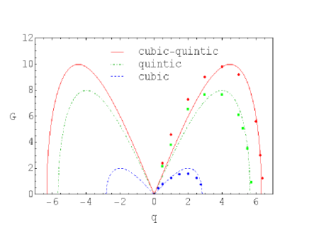
Figure 1: The growth rate of MI as a function of modulation wave number. When only the cubic nonlinearity is in action ($\lambda=1,\beta=1,\gamma=0$), the modulation of the plane waves with $|q|<2.7$ leads to its instability (blue dashed line). The quintic nonlinearity ($\lambda=0,\gamma=1,\alpha=1$) leads to instability in a wider region of modulation wave numbers $|q|<5.6$ (green dot-dashed line). The combined action of both nonlinearities ($\lambda=1,\beta=1,\gamma=1,\alpha=1$) further expands the domain of instability $|q|<6.3$ (red solid line). The wave number, corresponding to the maximum growth rate, also shifts to greater values. Numerical values of MI growth rates, obtained from Eq. (1) with weakly modulated ($u_{j}=v_{j}=0.01$) plane wave initial conditions and using Eq. (16), are represented by symbols. For negative values of the modulation wave number $q$ the data are symmetric with respect to the origin, hence not shown. Parameter values: $c_{1}=c_{2}=0.5,\,a_{1}=1.0,\,a_{2}=0.999$.

3 Numerical results

Numerical simulations are performed by standard split-step fast Fourier transform method [26] using 2048 Fourier modes [27] within the integration domain of length $x\in[-20\pi,20\pi]$, and the time step was $dt=0.001$. The spacial frequency of weak modulation of the plane waves $q$ has been selected so that the periodic boundary conditions for Eqs. (1) is satisfied (i.e. the integer number of modulation wave periods fits the integration domain). When considering the flat-top soliton initial conditions, we put absorbers at the domain boundaries [28] to prevent the interference of linear waves (emitted by solitons in the central part and subsequently reflected from the domain boundaries) with emerging localized structures. In fact, the absorbers emulate the unbounded system.

In Fig. 2 we present the results of numerical simulations of Eqs. (1) for different sets of parameters. When only the cubic nonlinear terms in the equations are preserved ($\lambda=1,\gamma=0$), periodic emergence of soliton trains in the system is observed, as shown in the left panel. Experimental observation of the associated Fermi-Pasta-Ulam recurrence phenomenon in propagation of modulationally unstable waves in optical fibers with Kerr type nonlinearity was reported in [29]. In contrast, when both types of nonlinearity are taken into account ($\lambda=1$, $\gamma=1$), the periodic emergence of soliton trains is compromised (right panel). In this case the soliton trains clearly emerge only two times, after that almost random distribution of pulse intensities sets in. We have shown the evolution of one component $\psi_{1}(x,t)$ of the system (1), because the other component $\psi_{2}(x,t)$ behaves similarly.

 

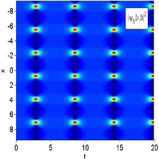
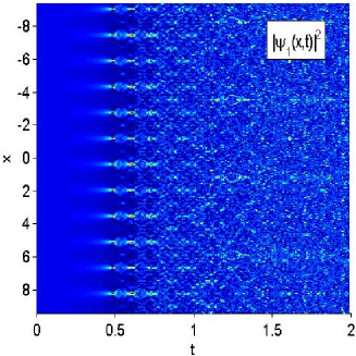
Figure 2: The results of numerical simulation of the governing Eqs. (1) with a weakly modulated plane wave initial conditions, given by Eqs. (4)-(5): $\psi_{j}(x)=a_{j}+\epsilon\sin(q_{j}x)$; $a_{1}=1.0$; $a_{2}=0.999$; $\epsilon=u_{j}=v_{j}=0.01$; $q_{1}=q_{2}=2.0$; $k_{j}=0$. Left panel: Only the cubic nonlinearity is in action $\lambda=1$, $\beta=1$, $\gamma=0$. Right panel: Both cubic and quintic nonlinearities are in action $\lambda=1$, $\beta=1$, $\gamma=1$, $\alpha=1$, $q_{1}=q_{2}=4.0$.

An important difference between the considered cases is that, the quintic and combined cubic-quintic nonlinearities give rise to solitons with bigger amplitude compared to those of cubic nonlinearity, as shown in Fig. 3. As expected, the higher order nonlinearity produces strongly compressed solitons and leads to cessation of the recurrence of soliton trains.

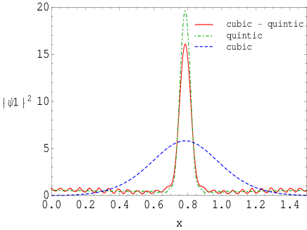
Figure 3: Solitons emerging from the MI when the instability is caused by different types of nonlinearities (only one pulse of the soliton train is shown for each type).

The linear stability analysis, described in the previous section, is valid only for the initial stage of MI. When the amplitude of perturbations becomes comparable with the background, the nonlinear stage of MI sets in, for which adequate theory has not been developed yet. However, some evidences are found for the universal behavior of waves emerging from MI in all media [10]. In particular, when localized perturbation is imposed upon the constant background, the evolving wave field distinctly divides into two outer regions, where the wave amplitude is the same as in unperturbed solution, and the central expanding oscillatory region. As a signature of the influence of quintic term on MI, we look for changes in this central oscillatory region of the integration domain.

For this purpose we impose a Gaussian localized perturbation on the background as in Ref. [3]

$$\psi(x,0)=1+i\exp(-x^{2})\cos(\sqrt{2}x).$$ (17)

Inserting this locally perturbed background solution as initial condition into Eq. (1), and propagating in time, we find clear changes due to the quintic term. The results are shown in Fig. 4.

 

 

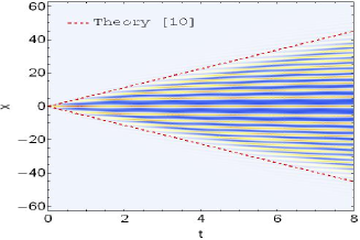
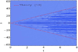
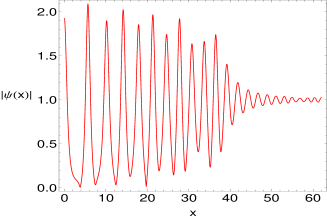
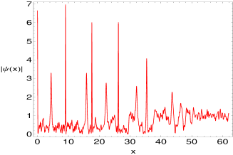
Figure 4: Top panels: Density plots of the wave field $|\psi(x,t)|$, evolving from locally perturbed initial condition Eq. (17) according to Eq. (1). Left: For single NLSE with cubic nonlinearity ($\lambda=2$, $\beta=0$, $\gamma=0$, $\alpha=0$) the oscillatory central region expands as predicted by theory [10] $\sim\pm 4\sqrt{2}\,t$ (red dashed lines). Right: For single NLSE with cubic-quintic nonlinearity ($\lambda=2$, $\beta=0$, $\gamma=0.5$, $\alpha=0$) the oscillatory region expands linearly with the same velocity, except emerging solitons are more compressed. Bottom panels: The solution $|\psi(x,t)|$ at $t=8$ for cubic (left) and cubic-quintic (right) NLSE.

The main difference in the nonlinear evolution of MI in cubic and cubic-quintic NLSE is that, in the latter case the emerging solitons are more compressed and evenly spaced (compare the bottom panels in Fig. 4). However, the universal feature of nonlinear MI in both media is preserved. Namely, the central oscillatory region of the wave field expands linearly with time, and the outer quiescent region is quite sharply separated from central oscillatory region of MI.

4 Coupled solitons emerging from MI

In the absence of inter-component interactions ($\alpha=0,\ \beta=0$) the system of Eqs. (1) splits into two independent NLS equations with cubic-quintic nonlinearity, which we present in a more convenient form by setting $c_{j}\rightarrow 1/2$, and $\gamma\rightarrow-\gamma$

$$i\psi_{t}+\frac{1}{2}\psi_{xx}+\lambda|\psi|^{2}\psi-\gamma|\psi|^{4}\psi=0.$$ (18)

An essential property of Eq. (18) is that it supports so called flat-top solitons [30, 31]

$$\psi(x) = \sqrt{\frac{3\lambda}{4\gamma}}\ \frac{{\rm tanh}(\eta)}{\sqrt{1+\mathrm{sech}(\eta)\mathrm{cosh}(x/a)}},$$ (19)

$$\qquad\eta = \sqrt{\frac{2\gamma}{3}},\quad a=\frac{\eta}{\lambda\mathrm{tanh}(\eta)},$$

a pedestal-shaped localized states which can propagate preserving their form and velocity, but collide with each-other inelastically [25].

Below we consider the MI in our system with flat-top soliton initial conditions in both components. Such a setting with vanishing boundary conditions is convenient for observing coupled solitons, emerging from MI and evolving in the domain of integration for extended period of time. Since the interaction between flat-top solitons is a strong perturbation, substantial amount of radiation of linear waves will take place during the process. These linear waves have to be removed from the integration domain since they can be reflected from the domain boundaries and hence interfere with emerging structures in its central part. For this purpose we use the technique of absorbing boundaries proposed in [28]. A similar setting with vanishing boundary conditions was employed in [32] to study the generation of symbiotic optical solitons in coupled system of NLSE with Kerr type nonlinearity.

To start the numerical simulations we introduce the following perturbed flat-top soliton initial conditions into Eqs. (1)

$$\psi_{j}(x,0)=\psi(x)[1+\epsilon_{j}\sin(qx)],\quad j=1,2,$$

with $\psi(x)$ given by Eq. (19). These two flat-top solitons are similar except for the weak perturbations with different amplitudes ($\epsilon_{j}$) imposed on them. The evolution of two interacting pulses (19), governed by Eqs. (1) is presented in Fig. 5. In order to have extended pedestal shaped pulses with sufficient background intensity, we use suitable values for the parameters $\lambda$ and $\gamma$ of the flat-top soliton. Estimation of these parameters for BEC of ⁸⁷Rb can be found in [33] As can be seen from this figure, MI fully develops around $t\sim 0.5$, after that emergence of coupled solitons takes place in the interval $t\in[2,5]$. Three coupled solitons fully developed and freely propagate when $t>5$. It should be noted, that formation of coupled solitons is possible when the norm of each soliton is big enough so that mutual attraction between them overcomes the quintic self-repulsion ($\lambda>0$, $\beta>0$, $\gamma<0$, $\alpha<0$). For this reason smaller pulse pairs to the left and right of the three central pulses disperse and leave the integration domain by $t\sim 10$.

 

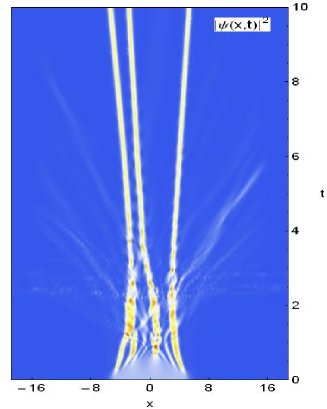
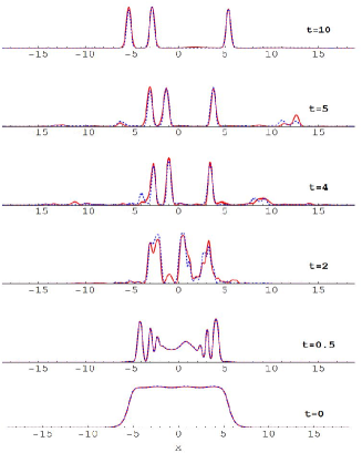
Figure 5: Formation of coupled solitons due to the phenomenon of MI in NLS Eqs. (1). The initial conditions are taken as weakly modulated flat-top solitons Eq. (4). Left panel: Density plot for the time evolution of the first component $|\psi_{1}(x,t)|^{2}$. The evolution of the second component is similar, that is why not shown. Right panel: The initial state ($t=0$) and several time sections for the evolution of the coupled system (1) under developing MI. Red solid line and blue dashed line correspond to the first and second components, respectively. Formation of three coupled solitons can be clearly observed. The length of integration domain $L=24\pi/q$ is selected to accommodate an integer number of modulation periods. Parameter values: $c=0.5$, $\lambda=100$, $\beta=1$, $\gamma=800$, $\alpha=-0.1$, $q=2$, $\epsilon_{1}=0.01$, $\epsilon_{2}=0.02$.

5 Conclusions

We have studied the phenomenon of MI in a two-component continuous system featuring cubic-quintic nonlinearity both in linear and nonlinear stages. For the linear stage analytic expression for the growth rate of MI has been derived and compared with the results of numerical simulations of the governing NLSE system. The model allows to identify the contribution of each type of nonlinearity on the overall growth rate of MI. It is found that the quintic nonlinearity significantly enhances the development of MI in these media and suppresses recurrence property of emerging soliton trains. To investigate MI in the nonlinear stage we use the evidence of a universal behavior, discovered in Ref. [10]. It appears, that the quintic nonlinearity leads to emergence of more compressed and evenly spaced solitons, while the expansion of the central oscillatory region obeys the same linear time dependence. In addition generation of coupled solitons of the bright-bright type resulted from MI of flat-top solitons has been investigated via numerical simulations. Obtained results can be useful in studies of binary mixtures of BEC with high density, where the three-body atomic interactions play a significant role, and of light propagation in optical materials with a large fifth-order nonlinearity.

References

- [1] V. E. Zakharov and L. A. Ostrovsky, Modulation instability: the beginning, Physica D: Nonlinear Phenomena 238(5), 540-548 (2009).
- [2] F. Kh. Abdullaev, S. A. Darmanyan, and J. Garnier, Modulational instability of electromagnetic waves in inhomogeneous and in discrete media, Progress in Optics. 44, 303-365 (2002).
- [3] G. Biondini, S. Li, D. Mantzavinos, S. Trillo, Universal behavior of modulationally unstable media, SIAM Review 60 (4), 888 908 (2018).
- [4] V. I. Bespalov and V. I. Talanov, Filamentary structure of light beams in nonlinear liquids, JETP Lett. 3, 307 (1966).
- [5] Y. Taniuti and H. Washimi, Self-trapping and instability of hydromagnetic waves along the magnetic field in a cold plasma, Phys. Rev. Lett. 21, 209 (1968).
- [6] T. B. Benjamin and J. E. Feir, The disintegration of wave-trains on deep water, J. Fluid Mech. 27, 417 (1967).
- [7] P. Marquie, J. M. Bilbault and M. Remoissenet, Generation of envelope and hole solitons in an experimental transmission line, Phys. Rev. E49, 828 (1994).
- [8] V. V. Konotop and M. Salerno, Modulational instability in Bose-Einstein condensates in optical lattices, Phys. Rev. A65, 021602(R) (2002); B. B. Baizakov, V. V. Konotop and M. Salerno, Regular spatial structures in arrays of Bose-Einstein condensates induced by modulational instability, J. Phys. B35, 5105 (2002).
- [9] V. E. Zakharov and A. A. Gelash, Nonlinear stage of modulation instability, Phys. Rev. Lett. 111, 054101 (2013).
- [10] G. Biondini and D. Mantzavinos, Universal nature of the nonlinear stage of modulational instability, Phys. Rev. Lett. 116, 043902 (2016).
- [11] N. Akhmediev, A. Ankiewicz and M. Taki, Waves that appear from nowhere and disappear without a trace, Phys. Lett. A373, 675 (2009).
- [12] A. Maluckov, L. Hadzievski, N. Lazarides and G. Tsironis, Extreme events in discrete nonlinear lattices, Phys. Rev. E79, 025601 (2009).
- [13] I. Ferrier-Barbut, M. Wenzel, M. Schmitt, F. Böttcher, and T. Pfau, Onset of a modulational instability in trapped dipolar Bose-Einstein condensates, Phys. Rev. A 97, 011604(R) (2018).
- [14] A. Hasegawa and Y. Kodama, Solitons in Optical Communications (Clarendon Press, Oxford, 1995).
- [15] K. E. Strecker,G. B. Partridge, A. G. Truscott and R. G. Hulet, Formation and propagation of matter-wave soliton trains , Nature 417, 150 (2002).
- [16] J. H. V. Nguyen, D. Luo, R. G. Hulet, Formation of matter-wave soliton trains by modulational instability, Science 356, 422 426 (2017).
- [17] H. Fabrelli, J. B. Sudharsan, R. Radha, A. Gammal and B. A. Malomed, Solitons under spatially localized cubic - quintic - septimal nonlinearities, J. Opt. 19, 075501 (2017).
- [18] M. Saha and A. K. Sarma, Modulation instability in nonlinear metamaterials induced by cubic - quintic nonlinearities and higher order dispersive effects, Optics Commun. 291, 321 325 (2013).
- [19] B. Baizakov, A. Bouketir, A. Messikh and B. Umarov, Modulational instability in two-component discrete media with cubic-quintic nonlinearity, Phys. Rev. E 79, 046605 (2009).
- [20] Y. S. Kivshar and D. K. Campbell, Peierls-Nabarro potential barrier for highly localized nonlinear modes, Phys. Rev. E 48, 3077-3081 (1993).
- [21] A. E. Kraych, P. Suret, G. El, and S. Randoux, Universal nonlinear stage of the locally induced modulational instability in fiber optics, arXiv preprint arXiv:1805.05074 (2018).
- [22] A. Maimistov, B. A. Malomed and A. Desyatnikov, A potential of incoherent attraction between multidimensional solitons, Phys. Lett. A 254, 179 (1999).
- [23] F. Smektala, C. Quemard, V. Couderc, and A. Barthélémy , Non-linear optical properties of chalcogenide glasses measured by Z-scan, J. Non-Cryst. Solids, 274, 232 (2000); G. Boudebs, S. Cherukulappurath , H. Leblond , J. Troles , F. Smektala , F. Sanchez, Experimental and theoretical study of higher-order nonlinearities in chalcogenide glasses, Opt. Commun. 219, 427 (2003).
- [24] B. Lawrence, W. E. Torruellas, M. Cha, M. L. Sundheimer, G. I. Stegeman, J. Meth, S. Etemad, and G. Baker, Identification and role of two-photon excited states in a conjugated Polymer, Phys. Rev. Lett. 73, 597 (1994).
- [25] S. O. Elyutin, Polarized optical pulses in a medium with third- and fifth-order nonlinearities, Opt. Spectrosc. 106, 407 (2009).
- [26] G. P. Agrawal, Nonlinear Fiber Optics (Academic Press, New York, 1995).
- [27] W. H. Press, S. A. Teukolsky, W. T. Vetterling and B. P. Flannery, Numerical Recipes : The Art of Scientific Computing (Cambridge University Press, Cambridge, 1996).
- [28] P. Berg, F. If, P. L. Christiansen, and O. Skovgaard, Soliton laser: A computational two - cavity model, Phys. Rev. A35, 4167 (1987).
- [29] G. V. Simaeys, Ph. Emplit and M. Haelterman, Experimental demonstration of the Fermi-Pasta-Ulam recurrence in a modulationally unstable optical wave, Phys. Rev. Lett. 87, 033902 (2001).
- [30] Kh. I. Pushkarov, D. I. Pushkarov and I. V. Tomov, Self-action of light beams in nonlinear media: soliton solutions, Opt. Quantum Electron. 11, 471 (1979).
- [31] A. I. Maimistov and A. M. Basharov, Nonlinear Optical Waves (Kluwer, Dordrecht, 1999).
- [32] Yu. S. Kivshar, D. Anderson, A Höök, M Lisak, A. A. Afanasjev and V. N. Serkin, Symbiotic optical solitons and modulational instability, Phys. Scr. 44, 195 (1991).
- [33] B. B. Baizakov, A. Bouketir, A. Messikh, A. Benseghir and B. A. Umarov, Variational analysis of flat-top solitons in Bose - Einstein condensates, Int. J. Mod. Phys. B18, 2427 (2011).