Angular distribution as an effective probe of new physics
in semi-hadronic three-body meson decays

Abstract

We analyze, in a fully model-independent manner, the effects of new physics on a few semi-hadronic three-body meson decays of the type $P_{i}\to P_{f}f_{1}f_{2}$, where $P_{i},P_{f}$ are well chosen pseudo-scalar mesons and $f_{1,2}$ denote fermions out of which at least one gets detected in experiments. We find that the angular distribution of events of these decays can probe many interesting new physics, such as the nature of the intermediate particle that can cause lepton-flavor violation, or presence of heavy sterile neutrino, or new intermediate particles, or new interactions. We also provide angular asymmetries which can quantify the effects of new physics in these decays. We illustrate the effectiveness of our proposed methodology with a few well chosen decay modes showing effects of certain new physics possibilities without any hadronic uncertainties.

I Introduction

New physics (NP), or physics beyond the standard model, involves various models that extend the well verified standard model (SM) of particle physics by introducing a number of new particles with novel properties and interactions. Though various aspects of many of these particles and interactions are constrained by existing experimental data, we are yet to detect any definitive signature of new physics in our experiments. Nevertheless, recent experimental studies in $B$ meson decays, such as $B\to K^{(*)}\ell^{-}\ell^{+}$ B2KorKstLL , $B_{s}\to\phi\ell^{-}\ell^{+}$ Aaij:2015esa , $B\to D^{(*)}\ell\nu$ B2DorDstLN and $B_{c}\to J/\psi\ell\nu$ Aaij:2017tyk (where $\ell$ can be $e,\mu$ or $\tau$) have reported anomalous observations raising the expectation of discovery of new physics with more statistical significance. In this context, model-independent studies of such semi-leptonic three-body meson decay processes become important as they can identify generic signatures of new physics which can be probed experimentally. In this paper, we have analyzed the effects of new physics, in a model-independent manner, on the angular distribution of a general semi-hadronic three-body meson decay of the type $P_{i}\to P_{f}f_{1}f_{2}$, where $P_{i}$ and $P_{f}$ are the initial and final pseudo-scalar mesons respectively, and $f_{1,2}$ denote fermions (which may or may not be leptons but not quarks) out of which at least one gets detected experimentally. Presence of new interactions, or new particles such as fermionic dark matter (DM) particles or heavy sterile neutrinos or long lived particles (LLP) would leave their signature in the angular distribution and we show by example how new physics contribution can be quantified from angular asymmetries. Our methodology can be used for detection of new physics in experimental study of various three-body pseudo-scalar meson decays at various collider experiments such as LHCb and Belle II.

The structure of our paper is as follows. In Sec. II we discuss the most general Lagrangian and amplitude which include all probable NP contributions to our process under consideration. The relevant details of kinematics is then described in Sec. III. This is followed by a discussion on the angular distribution and the various angular asymmetries in Sec. IV. In Sec. V we present a few well chosen examples illustrating the effects of new physics on the angular distribution. In Sec. VI we conclude by summarizing the important aspects of our methodology and its possible experimental realization.

II Most general Lagrangian and Amplitude

Following the model-independent analysis of the decay $B\to D\ell^{-}\ell^{+}$ as given in Ref. Kim:2016zbg and generalizing it for our process $P_{i}\to P_{f}f_{1}f_{2}$ where $P_{i,f}$ can be $B,B_{s},B_{c},D,K,\pi$ etc. as appropriate and $f_{1}f_{2}$ can be $\ell^{-}\ell^{+}$, $\ell\bar{\ell^{\prime}}$, $\ell\nu_{\ell}$, $\ell\nu_{S}$, $\ell f^{DM}$, $\nu_{\ell}\overline{\nu}_{\ell}$, $\nu_{S}\overline{\nu}_{\ell}$, $\nu_{\ell}\overline{\nu}_{S}$, $\nu_{S}\overline{\nu}_{S}$, $f^{DM}\bar{f}^{DM}$, $f_{1}^{DM}f_{2}^{DM}$, $f_{1}^{LLP}f_{2}^{LLP}$ (with $\ell,\ell^{\prime}=e,\mu,\tau$ denoting leptons, $\nu_{S}$ being sterile neutrino, $f^{DM}_{1,2}$ as fermionic dark matter and $f_{1,2}^{LLP}$ as long lived fermions), we can write down the effective Lagrangian facilitating the decay under consideration as follows,

$$\mathcal{L}_{\textrm{eff}} = J_{S}\left(\bar{f}_{1}f_{2}\right)+J_{P}\left(\bar{f}_{1}~{}\gamma^{5}~{}f_{2}\right)+\left(J_{V}\right)_{\alpha}\left(\bar{f}_{1}~{}\gamma^{\alpha}~{}f_{2}\right)$$ (1)

$$+\left(J_{A}\right)_{\alpha}\left(\bar{f}_{1}~{}\gamma^{\alpha}\gamma^{5}~{}f_{2}\right)+\left(J_{T_{1}}\right)_{\alpha\beta}\left(\bar{f}_{1}~{}\sigma^{\alpha\beta}~{}f_{2}\right)$$

$$+\left(J_{T_{2}}\right)_{\alpha\beta}\left(\bar{f}_{1}~{}\sigma^{\alpha\beta}\gamma^{5}~{}f_{2}\right)+\text{h.c.},$$

where $J_{S}$, $J_{P}$, $\left(J_{V}\right)_{\alpha}$, $\left(J_{A}\right)_{\alpha}$, $\left(J_{T_{1}}\right)_{\alpha\beta}$, $\left(J_{T_{2}}\right)_{\alpha\beta}$ are the different hadronic currents which effectively describe the quark level transitions from $P_{i}$ to $P_{f}$ meson. It should be noted that we have kept both $\sigma^{\alpha\beta}$ and $\sigma^{\alpha\beta}\gamma^{5}$ terms. This is because of the fact that the currents $\bar{f}_{1}\,\sigma^{\alpha\beta}\,f_{2}$ and $\bar{f}_{1}\,\sigma^{\alpha\beta}\gamma^{5}\,f_{2}$ describe two different physics aspects namely the magnetic dipole and electric dipole contributions respectively. In the SM, vector and axial-vector currents (mediated by photon, $W^{\pm}$ and $Z^{0}$ bosons) and the scalar current (mediated by Higgs boson) contribute. So every other term in Eq. (1) except the ones with $J_{S}$, $\left(J_{V}\right)_{\alpha}$ and $\left(J_{A}\right)_{\alpha}$ can appear in some specific NP model. Since, in this paper, we want to concentrate on a fully model-independent analysis to get generic signatures of new physics, we shall refrain from venturing into details of any specific NP model, which nevertheless are also useful. It is important to note that $J_{S}$, $\left(J_{V}\right)_{\alpha}$ and $\left(J_{A}\right)_{\alpha}$ can also get modified due to NP contributions.

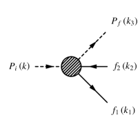
Figure 1: Feynman diagram for $P_{i}\to P_{f}f_{1}f_{2}$ considering $f_{1}$ as a particle and $f_{2}$ as an anti-particle. Here the blob denotes the effective vertex and includes contributions from all the form factors defined in Eq. (3).

In order to get the most general amplitude for our process under consideration, we need to go from the effective quark-level description of Eq. (1) to the meson level description by defining appropriate form factors. It is easy to write down the most general form of the amplitude for the process $P_{i}\to P_{f}f_{1}f_{2}$ depicted in Fig. 1 as follows,

$$\mathcal{M}\left(P_{i}\to P_{f}f_{1}f_{2}\right) =F_{S}\left(\bar{f}_{1}f_{2}\right)+F_{P}\left(\bar{f}_{1}~{}\gamma^{5}~{}f_{2}\right)$$

$$\quad+\left(F_{V}^{+}p_{\alpha}+F_{V}^{-}q_{\alpha}\right)\left(\bar{f}_{1}~{}\gamma^{\alpha}~{}f_{2}\right)$$

$$\quad+\left(F_{A}^{+}p_{\alpha}+F_{A}^{-}q_{\alpha}\right)\left(\bar{f}_{1}~{}\gamma^{\alpha}~{}\gamma^{5}~{}f_{2}\right)$$

$$\quad+F_{T_{1}}~{}p_{\alpha}~{}q_{\beta}\left(\bar{f}_{1}~{}\sigma^{\alpha\beta}~{}f_{2}\right)$$

$$\quad+F_{T_{2}}~{}p_{\alpha}~{}q_{\beta}\left(\bar{f}_{1}~{}\sigma^{\alpha\beta}~{}\gamma^{5}~{}f_{2}\right),$$ (2)

where $F_{S}$, $F_{P}$, $F_{V}^{\pm}$, $F_{A}^{\pm}$, $F_{T_{1}}$ and $F_{T_{2}}$ are the relevant form factors, and are defined as follows,

$$\langle P_{f}\lvert J_{S}\rvert P_{i}\rangle =F_{S},$$ (3a)

$$\langle P_{f}\lvert J_{P}\rvert P_{i}\rangle =F_{P},$$ (3b)

$$\langle P_{f}\lvert\left(J_{V}\right)_{\alpha}\rvert P_{i}\rangle =F_{V}^{+}p_{\alpha}+F_{V}^{-}q_{\alpha},$$ (3c)

$$\langle P_{f}\lvert\left(J_{A}\right)_{\alpha}\rvert P_{i}\rangle =F_{A}^{+}p_{\alpha}+F_{A}^{-}q_{\alpha},$$ (3d)

$$\langle P_{f}\lvert\left(J_{T_{1}}\right)_{\alpha\beta}\rvert P_{i}\rangle =F_{T_{1}}~{}p_{\alpha}~{}q_{\beta},$$ (3e)

$$\langle P_{f}\lvert\left(J_{T_{2}}\right)_{\alpha\beta}\rvert P_{i}\rangle =F_{T_{2}}~{}p_{\alpha}~{}q_{\beta},$$ (3f)

with $p\equiv k+k_{3}$ and $q\equiv k-k_{3}=k_{1}+k_{2}$, in which $k,k_{1},k_{2},k_{3}$ are the 4-momenta of the $P_{i},f_{1},f_{2}$ and $P_{f}$ respectively (see Fig. 1). All the form factors appearing in the amplitude in Eq. (2) and as defined in Eq. (3) are, in general, complex and contain all NP information. It should be noted that for simplicity we have implicitly put all the relevant Cabibbo-Kobayashi-Maskawa matrix elements as well as coupling constants and propagators inside the definitions of these form factors. In the SM only $F_{V}^{\pm}$ and $F_{A}^{\pm}$ are present. Presence of NP can modify these as well as introduce other form factors. These various NP contributions would leave behind their signatures in the angular distribution for which we need to specify the kinematics in a chosen frame of reference.

III Decay Kinematics

Figure 2: Decay of $P_{i}\to P_{f}f_{1}f_{2}$ in the Gottfried-Jackson frame.

We shall consider the decay $P_{i}\to P_{f}f_{1}f_{2}$ in the Gottfried-Jackson frame, especially the center-of-momentum frame of the $f_{1},f_{2}$ system, which is shown in Fig. 2. In this frame the parent meson $P_{i}$ flies along the positive $z$-direction with 4-momentum $k=\left(E,\mathbf{k}\right)=\left(E,0,0,\left|\mathbf{k}\right|\right)$ and decays to the daughter meson $P_{f}$ which also flies along the positive $z$-direction with 4-momentum $k_{3}=\left(E_{3},\mathbf{k}_{3}\right)=\left(E_{3},0,0,\left|\mathbf{k}_{3}\right|\right)$ and to $f_{1}$, $f_{2}$ which fly away back-to-back with 4-momenta $k_{1}=\left(E_{1},\mathbf{k}_{1}\right)$ and $k_{2}=\left(E_{2},\mathbf{k}_{2}\right)$ respectively, such that by conservation of 4-momentum we get, $\mathbf{k}_{1}+\mathbf{k}_{2}=\mathbf{0}$, $\mathbf{k}=\mathbf{k}_{3}$, and $E=E_{1}+E_{2}+E_{3}$. The fermion $f_{1}$ (which we assume can be observed experimentally) flies out subtending an angle $\theta$ with respect to the direction of flight of the $P_{i}$ meson, in this Gottfried-Jackson frame. The three invariant mass-squares involved in the decay under consideration are defined as follows,

$$s =(k_{1}+k_{2})^{2}=(k-k_{3})^{2},$$ (4a)

$$t =(k_{1}+k_{3})^{2}=(k-k_{2})^{2},$$ (4b)

$$u =(k_{2}+k_{3})^{2}=(k-k_{1})^{2}.$$ (4c)

It is easy to show that $s+t+u=m_{i}^{2}+m_{f}^{2}+m_{1}^{2}+m_{2}^{2}$, where $m_{i},m_{f},m_{1}$ and $m_{2}$ denote the masses of particles $P_{i},P_{f},f_{1}$ and $f_{2}$ respectively. In the Gottfried-Jackson frame, the expressions for $t$ and $u$ are given by

$$t =a_{t}-b\cos\theta,$$ (5a)

$$u =a_{u}+b\cos\theta,$$ (5b)

where

$$a_{t} =m_{1}^{2}+m_{f}^{2}+\frac{1}{2s}\left(s+m_{1}^{2}-m_{2}^{2}\right)\left(m_{i}^{2}-m_{f}^{2}-s\right),$$ (6a)

$$a_{u} =m_{2}^{2}+m_{f}^{2}+\frac{1}{2s}\left(s-m_{1}^{2}+m_{2}^{2}\right)\left(m_{i}^{2}-m_{f}^{2}-s\right),$$ (6b)

$$b =\frac{1}{2s}\sqrt{\lambda\left(s,m_{1}^{2},m_{2}^{2}\right)~{}\lambda\left(s,m_{i}^{2},m_{f}^{2}\right)},$$ (6c)

with the Källén function $\lambda(x,y,z)$ defined as,

$$\lambda\left(x,y,z\right)=x^{2}+y^{2}+z^{2}-2\left(xy+yz+zx\right).$$

It is clear that $a_{t}$, $a_{u}$ and $b$ are functions of $s$ only. For the special case of $m_{1}=m_{2}=m$ (say) we have $a_{t}=a_{u}=\tfrac{1}{2}\left(m_{i}^{2}+m_{f}^{2}+2m^{2}-s\right)$ and $b=\tfrac{1}{2}\sqrt{\left(1-4m^{2}/s\right)\lambda\left(s,m_{i}^{2},m_{f}^{2}\right)}$. It is important to note that we shall use the angle $\theta$ in our angular distribution.

IV Most general angular distribution and angular asymmetries

Considering the amplitude as given in Eq. (2), the most general angular distribution in the Gottfried-Jackson frame is given by,

$$\frac{d^{2}\Gamma}{ds\,d\cos\theta}=\frac{b\sqrt{s}\left(C_{0}+C_{1}\cos\theta+C_{2}\cos^{2}\theta\right)}{128\,\pi^{3}\,m_{i}^{2}\left(m_{i}^{2}-m_{f}^{2}+s\right)},$$ (7)

where $C_{0}$, $C_{1}$ and $C_{2}$ are functions of $s$ and are given by,

$$C_{0} =2\Bigg{(}-\left|F_{T_{1}}\right|^{2}\bigg{(}-\Sigma m_{12}^{2}s^{2}+2\Sigma m_{12}^{2}\left(\Sigma m^{2}\right)_{if}s$$

$$\hskip 42.67912pt+\left(\Delta m^{2}\right)_{12}^{2}s-\Delta a_{tu}^{2}s-2\left(\Delta m^{2}\right)_{12}^{2}\left(\Sigma m^{2}\right)_{if}$$

$$\hskip 42.67912pt-\left(\Delta m^{2}\right)_{if}^{2}\Sigma m_{12}^{2}+2\Delta a_{tu}\left(\Delta m^{2}\right)_{12}\left(\Delta m^{2}\right)_{if}\bigg{)}$$

$$\quad-2\text{Im}\left(F_{V}^{+}F_{T_{1}}^{*}\right)\bigg{(}-\Sigma m_{12}s^{2}+2\Sigma m_{12}\left(\Sigma m^{2}\right)_{if}s$$

$$\hskip 42.67912pt+\Delta m_{12}\left(\Delta m^{2}\right)_{12}s-2\Delta m_{12}\left(\Delta m^{2}\right)_{12}\left(\Sigma m^{2}\right)_{if}$$

$$\hskip 42.67912pt-\left(\Delta m^{2}\right)_{if}^{2}\Sigma m_{12}+\Delta a_{tu}\Delta m_{12}\left(\Delta m^{2}\right)_{if}\bigg{)}$$

$$\quad+\left|F_{T_{2}}\right|^{2}\bigg{(}\Delta m_{12}^{2}s^{2}-2\Delta m_{12}^{2}\left(\Sigma m^{2}\right)_{if}s-\left(\Delta m^{2}\right)_{12}^{2}s$$

$$\hskip 42.67912pt+\Delta a_{tu}^{2}s+2\left(\Delta m^{2}\right)_{12}^{2}\left(\Sigma m^{2}\right)_{if}+\Delta m_{12}^{2}\left(\Delta m^{2}\right)_{if}^{2}$$

$$\hskip 42.67912pt-2\Delta a_{tu}\left(\Delta m^{2}\right)_{12}\left(\Delta m^{2}\right)_{if}\bigg{)}$$

$$\quad-2\text{Im}\left(F_{A}^{+}F_{T_{2}}^{*}\right)\bigg{(}\Delta m_{12}s^{2}-2\Delta m_{12}\left(\Sigma m^{2}\right)_{if}s$$

$$\hskip 42.67912pt-\left(\Delta m^{2}\right)_{12}\Sigma m_{12}s+2\left(\Delta m^{2}\right)_{12}\Sigma m_{12}\left(\Sigma m^{2}\right)_{if}$$

$$\hskip 42.67912pt-\Delta a_{tu}\left(\Delta m^{2}\right)_{if}\Sigma m_{12}+\Delta m_{12}\left(\Delta m^{2}\right)_{if}^{2}\bigg{)}$$

$$\quad+\left|F_{A}^{+}\right|^{2}\bigg{(}s^{2}-2\left(\Sigma m^{2}\right)_{if}s-\Sigma m_{12}^{2}s$$

$$\hskip 42.67912pt+2\Sigma m_{12}^{2}\left(\Sigma m^{2}\right)_{if}+\left(\Delta m^{2}\right)_{if}^{2}-\Delta a_{tu}^{2}\bigg{)}$$

$$\quad+\left|F_{V}^{+}\right|^{2}\bigg{(}s^{2}-2\left(\Sigma m^{2}\right)_{if}s-\Delta m_{12}^{2}s$$

$$\hskip 42.67912pt+2\Delta m_{12}^{2}\left(\Sigma m^{2}\right)_{if}+\left(\Delta m^{2}\right)_{if}^{2}-\Delta a_{tu}^{2}\bigg{)}$$

$$\quad+\left|F_{A}^{-}\right|^{2}\left(\Sigma m_{12}^{2}s-\left(\Delta m^{2}\right)_{12}^{2}\right)$$

$$\quad-2\text{Re}\left(F_{P}F_{A}^{-*}\right)\left(\Sigma m_{12}s-\Delta m_{12}\left(\Delta m^{2}\right)_{12}\right)$$

$$\quad-\left|F_{V}^{-}\right|^{2}\left(\left(\Delta m^{2}\right)_{12}^{2}-\Delta m_{12}^{2}s\right)$$

$$\quad-2\text{Re}\left(F_{S}F_{V}^{-*}\right)\left(\left(\Delta m^{2}\right)_{12}\Sigma m_{12}-\Delta m_{12}s\right)$$

$$\quad-\left|F_{S}\right|^{2}\left(\Sigma m_{12}^{2}-s\right)-\left|F_{P}\right|^{2}\left(\Delta m_{12}^{2}-s\right)$$

$$\quad+2\text{Re}\left(F_{A}^{+}F_{A}^{-*}\right)\left(\left(\Delta m^{2}\right)_{if}\Sigma m_{12}^{2}-\Delta a_{tu}\left(\Delta m^{2}\right)_{12}\right)$$

$$\quad-2\text{Re}\left(F_{P}F_{A}^{+*}\right)\left(\left(\Delta m^{2}\right)_{if}\Sigma m_{12}-\Delta a_{tu}\Delta m_{12}\right)$$

$$\quad-2\text{Re}\left(F_{S}F_{V}^{+*}\right)\left(\Delta a_{tu}\Sigma m_{12}-\Delta m_{12}\left(\Delta m^{2}\right)_{if}\right)$$

$$\quad+2\text{Re}\left(F_{V}^{+}F_{V}^{-*}\right)\left(\Delta m_{12}^{2}\left(\Delta m^{2}\right)_{if}-\Delta a_{tu}\left(\Delta m^{2}\right)_{12}\right)\Bigg{)},$$ (8a)

$$C_{1} =8b\Bigg{(}\Delta m_{12}\left(\text{Im}\left(F_{V}^{-}F_{T_{1}}^{*}\right)s-\text{Re}\left(F_{P}F_{A}^{+*}\right)\right)$$

$$\hskip 42.67912pt+\Sigma m_{12}\Big{(}-\text{Im}\left(F_{A}^{-}F_{T_{2}}^{*}\right)s+\text{Re}\left(F_{S}F_{V}^{+*}\right)$$

$$\hskip 113.81102pt-\left(\Delta m^{2}\right)_{if}\text{Im}\left(F_{A}^{+}F_{T_{2}}^{*}\right)\Big{)}$$

$$\hskip 42.67912pt+\Delta a_{tu}\left(\left|F_{V}^{+}\right|^{2}+\left|F_{A}^{+}\right|^{2}\right)$$

$$\hskip 42.67912pt+\left(\text{Im}\left(F_{S}F_{T_{1}}^{*}\right)+\text{Im}\left(F_{P}F_{T_{2}}^{*}\right)\right)s$$

$$\hskip 42.67912pt+\left(\Delta m^{2}\right)_{12}\left(\text{Re}\left(F_{V}^{+}F_{V}^{-*}\right)+\text{Re}\left(F_{A}^{+}F_{A}^{-*}\right)\right)$$

$$\hskip 42.67912pt+\left(\Delta m^{2}\right)_{if}\Delta m_{12}\text{Im}\left(F_{V}^{+}F_{T_{1}}^{*}\right)\Bigg{)},$$ (8b)

$$C_{2} =8b^{2}\left(\left(\left|F_{T_{2}}\right|^{2}+\left|F_{T_{1}}\right|^{2}\right)s-\left|F_{V}^{+}\right|^{2}-\left|F_{A}^{+}\right|^{2}\right),$$ (8c)

with

$$\Delta a_{tu} =a_{t}-a_{u},$$ (9a)

$$\Delta m_{12} =m_{1}-m_{2},$$ (9b)

$$\Delta m_{if} =m_{i}-m_{f},$$ (9c)

$$\Sigma m_{12} =m_{1}+m_{2},$$ (9d)

$$\Sigma m_{if} =m_{i}+m_{f},$$ (9e)

$$\left(\Delta m^{2}\right)_{12} =\Delta m_{12}\Sigma m_{12}=m_{1}^{2}-m_{2}^{2},$$ (9f)

$$\left(\Delta m^{2}\right)_{if} =\Delta m_{if}\Sigma m_{if}=m_{i}^{2}-m_{f}^{2},$$ (9g)

$$\left(\Sigma m^{2}\right)_{if} =m_{i}^{2}+m_{f}^{2}.$$ (9h)

In the limit $m_{1}=m_{2}$, which happens when $f_{1}f_{2}=\ell^{-}\ell^{+},\nu\overline{\nu},$ or $f^{DM}\bar{f}^{DM}$ etc., our expressions for the angular distribution matches with the corresponding expression in Ref. Kim:2016zbg . It is important to remember that in the SM we come across scalar, vector and axial vector currents only. Therefore, in the SM, $F_{P}^{\text{SM}}=F_{T_{1}}^{\text{SM}}=F_{T_{2}}^{\text{SM}}=0$, which implies that,

$$C_{0}^{\text{SM}}= 2\Bigg{(}\left|\left(F_{A}^{+}\right)_{\text{SM}}\right|^{2}\bigg{(}s^{2}-2\left(\Sigma m^{2}\right)_{if}s-\Sigma m_{12}^{2}s$$

$$\hskip 56.9055pt+2\Sigma m_{12}^{2}\left(\Sigma m^{2}\right)_{if}+\left(\Delta m^{2}\right)_{if}^{2}-\Delta a_{tu}^{2}\bigg{)}$$

$$\quad+\left|\left(F_{V}^{+}\right)_{\text{SM}}\right|^{2}\bigg{(}s^{2}-2\left(\Sigma m^{2}\right)_{if}s-\Delta m_{12}^{2}s$$

$$\hskip 64.01869pt+2\Delta m_{12}^{2}\left(\Sigma m^{2}\right)_{if}+\left(\Delta m^{2}\right)_{if}^{2}-\Delta a_{tu}^{2}\bigg{)}$$

$$\quad+\left|\left(F_{A}^{-}\right)_{\text{SM}}\right|^{2}\left(\Sigma m_{12}^{2}s-\left(\Delta m^{2}\right)_{12}^{2}\right)$$

$$\quad-\left|\left(F_{V}^{-}\right)_{\text{SM}}\right|^{2}\left(\left(\Delta m^{2}\right)_{12}^{2}-\Delta m_{12}^{2}s\right)$$

$$\quad-\left|\left(F_{S}\right)_{\text{SM}}\right|^{2}\left(\Sigma m_{12}^{2}-s\right)$$

$$\quad+2\text{Re}\left(\left(F_{A}^{+}\right)_{\text{SM}}\left(F_{A}^{-}\right)_{\text{SM}}^{*}\right)\bigg{(}\left(\Delta m^{2}\right)_{if}\Sigma m_{12}^{2}$$

$$\hskip 113.81102pt-\Delta a_{tu}\left(\Delta m^{2}\right)_{12}\bigg{)}$$

$$\quad+2\text{Re}\left(\left(F_{V}^{+}\right)_{\text{SM}}\left(F_{V}^{-}\right)_{\text{SM}}^{*}\right)\bigg{(}\left(\Delta m^{2}\right)_{if}\Delta m_{12}^{2}$$

$$\hskip 113.81102pt-\Delta a_{tu}\left(\Delta m^{2}\right)_{12}\bigg{)}\Bigg{)},$$ (10a)

$$C_{1}^{\text{SM}}= 8b\Bigg{(}\Delta a_{tu}\left(\left|\left(F_{V}^{+}\right)_{\text{SM}}\right|^{2}+\left|\left(F_{A}^{+}\right)_{\text{SM}}\right|^{2}\right)$$

$$\qquad+\left(\Delta m^{2}\right)_{12}\bigg{(}\text{Re}\left(\left(F_{V}^{+}\right)_{\text{SM}}\left(F_{V}^{-}\right)_{\text{SM}}^{*}\right)$$

$$\hskip 71.13188pt+\text{Re}\left(\left(F_{A}^{+}\right)_{\text{SM}}\left(F_{A}^{-}\right)_{\text{SM}}^{*}\right)\bigg{)}\Bigg{)},$$ (10b)

$$C_{2}^{\text{SM}}= -8b^{2}\left(\left|\left(F_{V}^{+}\right)_{\text{SM}}\right|^{2}+\left|\left(F_{A}^{+}\right)_{\text{SM}}\right|^{2}\right).$$ (10c)

It is interesting to note that in the special case of $m_{1}=m_{2}$, such as in $P_{i}\to P_{f}\ell^{+}\ell^{-}$, we always have $C_{1}^{\text{SM}}=0$. For specific meson decays of the form $P_{i}\to P_{f}f_{1}f_{2}$ allowed in the SM, one can write down $\left(F_{S}\right)_{\text{SM}}$ , $\left(F_{V}^{\pm}\right)_{\text{SM}}$ and $\left(F_{A}^{\pm}\right)_{\text{SM}}$, at least in principle. The SM prediction for the angular distribution can thus be compared with corresponding experimental measurement. In order to quantitatively compare the theoretical prediction with experimental measurement, we define the following three angular asymmetries which can precisely probe $C_{0}$, $C_{1}$ and $C_{2}$ individually,

$$A_{0}\equiv A_{0}(s) =\frac{-\frac{1}{6}\left(\int_{-1}^{-1/2}-7\int_{-1/2}^{+1/2}+\int_{+1/2}^{+1}\right)\dfrac{d^{2}\Gamma}{ds\,d\cos\theta}d\cos\theta}{d\Gamma/ds}$$

$$=3C_{0}/\left(6C_{0}+2C_{2}\right),$$ (11a)

$$A_{1}\equiv A_{1}(s) =\frac{-\left(\int_{-1}^{0}-\int_{0}^{+1}\right)\dfrac{d^{2}\Gamma}{ds\,d\cos\theta}d\cos\theta}{d\Gamma/ds}$$

$$=3C_{1}/\left(6C_{0}+2C_{2}\right),$$ (11b)

$$A_{2}\equiv A_{2}(s) =\frac{2\left(\int_{-1}^{-1/2}-\int_{-1/2}^{+1/2}+\int_{+1/2}^{+1}\right)\dfrac{d^{2}\Gamma}{ds\,d\cos\theta}d\cos\theta}{d\Gamma/ds}$$

$$=3C_{2}/\left(6C_{0}+2C_{2}\right).$$ (11c)

The angular asymmetries of Eq. (11) are functions of $s$ and it is easy to show that $A_{2}=3\left(1/2-A_{0}\right)$. We can do the integration over $s$ in Eq. (7) and define the following normalized angular distribution,

$$\frac{1}{\Gamma}\frac{d\Gamma}{d\cos\theta}=T_{0}+T_{1}\cos\theta+T_{2}\cos^{2}\theta,$$ (12)

where

$$T_{j}=3c_{j}/\left(6c_{0}+2c_{2}\right),$$ (13)

for $j=0,1,2$ and with

$$c_{j}=\int_{(m_{1}+m_{2})^{2}}^{(m_{i}-m_{f})^{2}}\frac{b\sqrt{s}\,C_{j}}{128\pi^{3}m_{i}^{2}\left(m_{i}^{2}-m_{f}^{2}+s\right)}ds.$$ (14)

From Eq. (13) it is easy to show that $T_{2}=3\left(1/2-T_{0}\right)$ which also ensures that integration over $\cos\theta$ on Eq. (12) is equal to $1$. It is interesting to note that the angular distribution of Eq. (12) can be written in terms of the orthogonal Legendre polynomials of $\cos\theta$ as well,

$$\frac{1}{\Gamma}\frac{d\Gamma}{d\cos\theta}=\sum_{i=0}^{2}\langle G^{(i)}\rangle P_{i}\left(\cos\theta\right).$$ (15)

Here we have followed the notation of Ref. Gratrex:2015hna which also analyzes decays of the type $P_{i}\to P_{f}f_{1}f_{2}$, with only leptons for $f_{1,2}$, in a model-independent manner but using a generalized helicity amplitude method. The observables $\langle G^{(i)}\rangle$ of Eq. (15) are related to $T_{0}$, $T_{1}$ and $T_{2}$ of Eq. (12) as follows,

$$\langle G^{(0)}\rangle =T_{0}+T_{2}/3=1/2,$$ (16a)

$$\langle G^{(1)}\rangle =T_{1},$$ (16b)

$$\langle G^{(2)}\rangle =2T_{2}/3.$$ (16c)

These angular observables $\langle G^{(i)}\rangle$’s can be obtained by using the method of moments Gratrex:2015hna ; Beaujean:2015xea . Another important way to describe the normalized angular distribution is by using a flat term $F_{H}/2$ and the forward-backward asymmetry $A_{FB}$ AngDist:Hiller as follows,

$$\frac{1}{\Gamma}\frac{d\Gamma}{d\cos\theta}=\frac{1}{2}F_{H}+A_{FB}\cos\theta+\frac{3}{4}\left(1-F_{H}\right)\left(1-\cos^{2}\theta\right).$$ (17)

This form of the angular distribution has also been used in the experimental community AngDist:Expt in the study of $B\to K\ell^{+}\ell^{-}$. The parameters $F_{H}$ and $A_{FB}$ are related to $T_{0}$, $T_{1}$ and $T_{2}$ as follows,

$$F_{H} =2\left(T_{0}+T_{2}\right)=3-4T_{0},$$ (18a)

$$A_{FB} =T_{1}.$$ (18b)

Thus we have shown that Eqs. (12), (15) and (17) are equivalent to one another. In this paper, we choose to work using the normalized angular distribution in terms of $T_{0}$, $T_{1}$ and $T_{2}$ as shown in Eq. (12). This is because the terms $T_{0}$, $T_{1}$ and $T_{2}$ can be easily determined experimentally by using the $t$-vs-$u$ Dalitz plot which does not depend on any specific frame of reference. This Dalitz plot can be easily divided into four segments $I$, $II$, $III$ and $IV$ as shown in Fig. 3. The segments are decided as follows,

Segment $I$	:	$-1\leqslant\cos\theta\leqslant-0.5$,
Segment $II$	:	$-0.5<\cos\theta\leqslant 0$,
Segment $II$	:	$0<\cos\theta\leqslant 0.5$,
Segment $IV$	:	$0.5<\cos\theta\leqslant 1$.

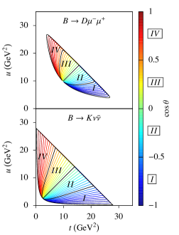
Figure 3: Two examples depicting the variation of $\cos\theta$ in the interior region of the $t$-vs-$u$ Dalitz plot. The interior of the Dalitz plot can be divided into four segments, $I$, $II$, $III$ and $IV$, as shown here.

The terms $T_{0}$, $T_{1}$ and $T_{2}$ can thus be expressed in terms of the following asymmetries,

$$T_{0} =-\frac{1}{6}\left(\frac{N_{I}-7\left(N_{II}+N_{III}\right)+N_{IV}}{N_{I}+N_{II}+N_{III}+N_{IV}}\right),$$ (19a)

$$T_{1} =\frac{\left(N_{I}+N_{II}\right)-\left(N_{III}+N_{IV}\right)}{N_{I}+N_{II}+N_{III}+N_{IV}},$$ (19b)

$$T_{2} =2\left(\frac{N_{I}-\left(N_{II}+N_{III}\right)+N_{IV}}{N_{I}+N_{II}+N_{III}+N_{IV}}\right),$$ (19c)

where $N_{j}$ denotes the number of events contained in the segment $j$. Since the $t$-vs-$u$ Dalitz plot does not depend on the frame of reference, we need not constraint ourselves to the Gottfried-Jackson frame of Fig. 2 and can work in the laboratory frame as well. Furthermore, we can use the expressions in Eq. (19) to search for NP.

V Illustrating the effects of new physics on the angular distribution

V.1 Classification of the $P_{i}\to P_{f}f_{1}f_{2}$ decays

It should be emphasized that for our methodology to work, we need to know the angle $\theta$ in the Gottfried-Jackson frame, or equivalently the $t$-vs-$u$ Dalitz plot, which demand that 4-momenta of the final particles be fully known. Usually, the 4-momenta of the initial and final pseudo-scalar mesons are directly measured experimentally. However, depending on the detection possibilities of $f_{1}$ and $f_{2}$ we can identify three distinct scenarios for our process $P_{i}\to P_{f}f_{1}f_{2}$. We introduce the notations $f_{i}^{\textrm{\char 51}}$ and $f_{i}^{\textrm{\char 55}}$ to denote whether the fermion $f_{i}$ gets detected (✓) or not (✗) by the detector. Using this notation the three scenarios are described as follows.

1. $P_{i}\to P_{f}+f_{1}^{\textrm{\char 51}}+f_{2}^{\textrm{\char 51}}\equiv P_{f}+\textrm{`visible'}$. Here both $f_{1}$ and $f_{2}$ are detected, e.g. when $f_{1}f_{2}=\ell^{-}\ell^{+}$ or $\ell\bar{\ell^{\prime}}$.

2. $P_{i}\to\begin{Bmatrix}P_{f}+f_{1}^{\textrm{\char 51}}+f_{2}^{\textrm{\char 55}}\\ P_{f}+f_{1}^{\textrm{\char 55}}+f_{2}^{\textrm{\char 51}}\end{Bmatrix}\equiv P_{f}+\textrm{`visible'}+\text{`invisible'}$. Here either $f_{1}$ or $f_{2}$ gets detected, e.g. when $f_{1}f_{2}=\ell\nu_{\ell}$, $\ell\nu_{S}$, $\ell f^{DM}$, $\ell f^{LLP}$.

3. $P_{i}\to P_{f}+f_{1}^{\textrm{\char 55}}+f_{2}^{\textrm{\char 55}}\equiv P_{f}+\textrm{`invisible'}$. Here neither $f_{1}$ nor $f_{2}$ gets detected, e.g. when $f_{1}f_{2}=\nu_{\ell}\overline{\nu}_{\ell}$, $\nu_{\ell}\overline{\nu}_{S}$, $\nu_{S}\overline{\nu}_{\ell}$, $\nu_{S}\overline{\nu}_{S}$, $f^{DM}\bar{f}^{DM}$, $f_{1}^{DM}f_{2}^{DM}$, $f_{1}^{LLP}f_{2}^{LLP}$ etc.

It should be noted that the above classification is based on our existing experimental explorations. What is undetected today might get detected in future with advanced detectors. In such a case we can imagine that, in future, the modes grouped in S2 might migrate to S1 and those in S3 might be grouped under S2. Below we explore each of the above scenarios in more details.

V.2 Exploration of new physics effects in each scenario

The first scenario (S1) is an experimenter’s delight as in this case all final 4-momenta can be easily measured and the $t$-vs-$u$ Dalitz plot can be obtained. Here, our methodology can be used to look for the possible signature of new physics in rare decays such as $B\to D\ell^{-}\ell^{+}$ (which can be found in Kim:2016zbg ) or study the nature of new physics contributing to lepton-flavor violating processes such as $B\to P\ell^{\pm}\ell^{\prime\mp}$ where $P=\pi,K,D$, $\ell\neq\ell^{\prime}$ and $\ell,\ell^{\prime}=e,\mu,\tau$. Let us consider a few NP possibilities mediating this lepton-flavor violating decay. There is no contribution within the SM to such decays. Therefore, all contribution to these decays comes from NP alone. It is very easy to note that for the decay $B\to P\ell^{-}\ell^{\prime+}$, from Eqs. (8) and (12) we get,

$$\frac{1}{\Gamma}\frac{d\Gamma}{d\cos\theta}=\begin{cases}\dfrac{1}{2},&\left(\parbox{99.73074pt}{{\centering only scalar or pseudo-scalar interaction\@add@centering}}\right)\\[14.22636pt] T_{0}+T_{2}\cos^{2}\theta,&\left(\parbox{99.73074pt}{{\centering only tensorial interaction\@add@centering}}\right)\\[8.53581pt] T_{0}+T_{1}\cos\theta+T_{2}\cos^{2}\theta,&\left(\parbox{99.73074pt}{{\centering only vector or axial-vector interaction\@add@centering}}\right)\end{cases}$$ (20)

where $T_{2}=3\left(1/2-T_{0}\right)$ with the quantities $T_{0}$, $T_{1}$ and $T_{2}$ being easily obtainable from the Dalitz plot distribution by using Eq. (19). It is clear from Eq. (20) that scalar or pseudo-scalar interaction would give rise to a uniform (or constant) angular distribution, while tensorial interaction gives a non-uniform distribution which is symmetric under $\cos\theta\leftrightarrow-\cos\theta$ and for this $T_{0}\leqslant 1/2$. On the other hand vector or axial-vector interaction can only be described by the most general form of the angular distribution, with its signature being $T_{1}\neq 0$. Nevertheless, if vector or axial-vector interaction contributes to the flavor violating processes $B\to P\ell^{-}\ell^{\prime+}$, it is important to note that $T_{1}\propto\left(m_{\ell}^{2}-m_{\ell^{\prime}}^{2}\right)$, where $m_{\ell}$, $m_{\ell^{\prime}}$ denote the masses of the charged leptons $\ell^{-}$ and $\ell^{\prime+}$ respectively. Therefore, we should observe an increase in the value of $T_{1}$ when going from $B\to P\mu^{-}e^{+}$ to $B\to P\tau^{-}\mu^{+}$ to $B\to P\tau^{-}e^{+}$. This would nail down the vector or axial vector nature of the NP, if it is the only NP contributing to these decays. Thus far we have analyzed the first scenario (S1) in which the relevant decays can be easily probed with existing detectors.

The second scenario (S2) can also be studied experimentally with existing detectors. In this case, the missing 4-momentum can be fully deduced using conservation of 4-momentum. Thus the $t$-vs-$u$ Dalitz plot can readily be obtained. Using our methodology the signatures of NP can then be extracted. One promising candidate for search for NP in this kind of scenario is in the decay $B\to P\ell N$ where $P=\pi$, $K$ or $D$ and $N$ can be an active neutrino ($\nu_{\ell}$) or sterile neutrino ($\nu_{S}$) or a neutral dark fermion ($f^{DM}$) or a long lived neutral fermion ($f^{LLP}$) which decays outside the detector. These S2 decay modes offer an exciting opportunity for study of NP effects.

The third scenario (S3), which has the maximum number of NP possibilities, is also the most challenging one for the current generation of experimental facilities, due to lack of information about the individual 4-momentum of $f_{1}$ and $f_{2}$. This implies that we can not do any angular analysis for these kind of decays unless by some technological advancement such as by using displaced vertex detectors we can manage to make measurement of the 4-momentum or the angular information of at least one of the final fermions. Getting 4-momenta of both the fermions would be ideal, but knowing 4-momentum of either one of them would suffice for our purpose. We are optimistic that the advancement in detector technology would push the current S3 decay modes to get labelled as S2 modes in the foreseeable future. It is important to note that once the current S3 modes enter the S2 category, we can cover the whole spectrum of NP possibilities in the $P_{i}\to P_{f}f_{1}f_{2}$ decays. Below we make a comprehensive exploration of NP possibilities in the generalized S2 decay modes, which includes the current S2 and S3 modes together.

V.3 Probing effects of new physics in the (S2)
and generalized (S2) scenarios

In the generalized S2 (GS2) scenario we have decays of the type $P_{i}\to\begin{Bmatrix}P_{f}+f_{1}^{\textrm{\char 51}}+f_{2}^{\textrm{\char 55}}\\ P_{f}+f_{1}^{\textrm{\char 55}}+f_{2}^{\textrm{\char 51}}\end{Bmatrix}\equiv P_{f}+\textrm{`visible'}+\text{`invisible'}$, where the detected (✓) or undetected (✗) nature is not constrained by our existing detector technology. In some cases, even with advanced detectors, either of the fermions $f_{1}$, $f_{2}$ might not get detected simply because its direction of flight lies outside the finite detector coverage, especially when the detector is located farther from the place of origin of the particle. Such possibilities are also included here. As noted before, measuring the 4-momentum of either of the final fermions would suffice to carry out the angular analysis following our approach.

In this context let us analyze the following decays.

1. S2 decay: $B\to P\ell^{-}f^{\textrm{\char 55}}$ where $P$ can be $\pi$ or $D$ and $f^{\textrm{\char 55}}$ is a neutral fermion. In the SM this process is mediated by $W^{-}$ boson and we have $f^{\textrm{\char 55}}=\overline{\nu}_{\ell}$. Presence of NP can imply $f^{\textrm{\char 55}}$ being a sterile neutrino $\nu_{S}$ or a fermionic dark matter particle $f^{DM}$ or a long lived fermion $f^{LLP}$, with additional non-SM interactions.

2. GS2 decay: $B\to Kf_{1}^{\textrm{\char 51}}f_{2}^{\textrm{\char 55}}$ where $f_{1}^{\textrm{\char 51}}$ and $f_{2}^{\textrm{\char 55}}$ are both neutral fermions. In the SM this process is mediated by $Z^{0}$ boson and we have $f_{1}f_{2}=\nu_{\ell}\overline{\nu}_{\ell}$. However, in case of NP contribution we can get pairs of sterile neutrinos or fermionic dark matter or fermionic long lived particles etc. along with nonstandard interactions as well. Here we are assuming that either of the final neutral fermions leaves a displaced vertex signature in an advanced detector so that its 4-momentum or angular information could be obtained.

V.3.1 New physics effects in the S2 decay $B\to P\ell^{-}f^{\textrm{\char 55}}$

Analyzing the $B\to P\ell^{-}f^{\textrm{\char 55}}$ decay in the SM we find that only vector and axial vector currents contribute and $F_{A}^{\pm}=-F_{V}^{\pm}$ while other form factors are zero. Also considering the anti-neutrino to be massless, i.e. $m_{2}=0$ we find that

$$a_{t} =m_{\ell}^{2}+m_{P}^{2}+\left(s+m_{\ell}^{2}\right)\left(m_{B}^{2}-m_{P}^{2}-s\right)/(2s),$$

$$a_{u} =m_{P}^{2}+\left(s-m_{\ell}^{2}\right)\left(m_{B}^{2}-m_{P}^{2}-s\right)/(2s),$$

$$b =\left(s-m_{\ell}^{2}\right)\sqrt{\lambda\left(s,m_{B}^{2},m_{P}^{2}\right)}/(2s),$$

where $m_{\ell}$, $m_{P}$ and $m_{B}$ denote the masses of the charged lepton $\ell^{-}$, mesons $P$ and $B$ respectively. Substituting these information in Eqs. (10) and in Eq. (7) we get,

$$\frac{d^{2}\Gamma^{\textrm{SM}}}{ds\,d\cos\theta}=\frac{b\sqrt{s}\left(C_{0}^{\textrm{SM}}+C_{1}^{\textrm{SM}}\cos\theta+C_{2}^{\textrm{SM}}\cos^{2}\theta\right)}{128\,\pi^{3}\,m_{B}^{2}\left(m_{B}^{2}-m_{P}^{2}+s\right)},$$ (21)

where

$$C_{0}^{\text{SM}}= 4\Bigg{(}\left|\left(F_{V}^{+}\right)_{\text{SM}}\right|^{2}\bigg{(}\lambda\left(s,m_{B}^{2},m_{P}^{2}\right)-m_{\ell}^{2}\left(s-2\left(m_{B}^{2}-m_{P}^{2}\right)\right)$$

$$\hskip 56.9055pt-m_{\ell}^{4}\left(m_{B}^{2}-m_{P}^{2}\right)^{2}/s^{2}\bigg{)}$$

$$\quad+\left|\left(F_{V}^{-}\right)_{\text{SM}}\right|^{2}m_{\ell}^{2}\left(s-m_{\ell}^{2}\right)$$

$$\quad+2\text{Re}\left(\left(F_{V}^{+}\right)_{\text{SM}}\left(F_{V}^{-}\right)_{\text{SM}}^{*}\right)m_{\ell}^{2}\left(m_{B}^{2}-m_{P}^{2}\right)\left(1-\frac{m_{\ell}^{2}}{s}\right)\Bigg{)},$$ (22a)

$$C_{1}^{\text{SM}}= 16m_{\ell}^{2}b\Bigg{(}\left(\frac{m_{B}^{2}-m_{P}^{2}}{s}\right)\left|\left(F_{V}^{+}\right)_{\text{SM}}\right|^{2}+\text{Re}\left(\left(F_{V}^{+}\right)_{\text{SM}}\left(F_{V}^{-}\right)_{\text{SM}}^{*}\right)\Bigg{)},$$ (22b)

$$C_{2}^{\text{SM}}= -16b^{2}\left|\left(F_{V}^{+}\right)_{\text{SM}}\right|^{2}.$$ (22c)

It is important to notice that in Eq. (22) we have many terms in the expression for $C_{0}^{\textrm{SM}}$ that are proportional to some power of the lepton mass, while the entire $C_{1}^{\textrm{SM}}$ is directly proportional to $m_{\ell}^{2}$. If we compare the $m_{\ell}$ dependent and $m_{\ell}$ independent contributions in $C_{0}^{\textrm{SM}}$ we find that the dependent terms are suppressed by about a factor of $\mathcal{O}\left(2m_{\ell}^{2}/m_{B}^{2}\right)$ which is roughly $8\times 10^{-4}$ for muon and $2\times 10^{-8}$ for electron. Thus we can neglect these $m_{\ell}$ dependent terms in comparison with mass independent terms. Equivalently, we can consider the charged leptons such as electron and muon as massless fermions, when compared with the $B$ meson mass scale. In the limit $m_{\ell}\to 0$ the expression for angular distribution as given in Eq. (21) becomes much simpler,

$$\frac{d^{2}\Gamma^{\text{SM}}}{ds\,d\cos\theta}=\frac{b^{3}\sqrt{s}}{8\,\pi^{3}\,m_{B}^{2}\left(m_{B}^{2}-m_{P}^{2}+s\right)}\left|\left(F_{V}^{+}\right)_{\text{SM}}\right|^{2}\sin^{2}\theta.$$ (23)

Independent of the expression for $\left(F_{V}^{+}\right)_{\text{SM}}$, it is easy to show that the normalized angular distribution is given by,

$$\frac{1}{\Gamma^{\text{SM}}}\frac{d\Gamma^{\text{SM}}}{d\cos\theta}=\frac{3}{4}\sin^{2}\theta,$$ (24)

which implies that $T_{0}=3/4=-T_{2}$, $T_{1}=0$. Since the distribution of events in the Dalitz plot is symmetric under $\cos\theta\leftrightarrow-\cos\theta$, we have $N_{I}=N_{IV}$ and $N_{II}=N_{III}$ which automatically satisfies the condition $T_{1}=0$. If we solve $T_{0}=3/4=-T_{2}$, we find that the number of events in the different segments of the Dalitz plot (equivalently the number of events in the four distinct bins of $\cos\theta$) are related to one another by

$$\frac{N_{I}}{N_{II}}=\frac{5}{11}=\frac{N_{IV}}{N_{III}}.$$ (25)

Any significant deviation from this would imply presence of NP effects. To illustrate the effects of NP on the angular distribution in these types of decays, we consider two simple and specific NP possibilities. Here we assume the charged lepton to be massless ($m_{\ell}=0$) and the undetected fermion ($f^{\textrm{\char 55}}$) to have mass $m\neq 0$.

Scalar type new physics:

Considering the simplest scalar type NP scenario, with $F_{S}\neq 0$, $F_{P}=F_{V}^{\pm}=F_{A}^{\pm}=F_{T_{1}}=F_{T_{2}}=0$, we get

$$C_{0}^{\text{NP}}= 2\left(s-m^{2}\right)\left|F_{S}\right|^{2},$$

$$C_{1}^{\text{NP}}= 0=C_{2}^{\text{NP}}.$$

In other words, there is no angular dependence at all here, i.e.

$$\frac{d^{2}\Gamma^{\text{NP}}}{ds\,d\cos\theta}=\frac{b\sqrt{s}}{64\,\pi^{3}\,m_{B}^{2}\left(m_{B}^{2}-m_{P}^{2}+s\right)}\left(s-m^{2}\right)\left|F_{S}\right|^{2},$$

where $b=\left(s-m^{2}\right)\sqrt{\lambda\left(s,m_{B}^{2},m_{P}^{2}\right)}/(2s)$ and $m^{2}\leqslant s\leqslant\left(m_{B}-m_{P}\right)^{2}$. If we do the integration over $s$, then the normalized angular distribution is given by,

$$\frac{1}{\Gamma^{\text{NP}}}\frac{d\Gamma^{\text{NP}}}{d\cos\theta}=\frac{1}{2}.$$

In fact, if such a new physics were present, our observation of $B\to P+\ell^{-}+f^{\textrm{\char 55}}$ would have the following angular distribution,

$$\frac{d\Gamma}{d\cos\theta}=\Gamma^{\text{SM}}\left(\frac{3}{4}\sin^{2}\theta+\frac{1}{2}\epsilon_{0}\right),$$

where we have parametrized the new physics contribution in terms of $\epsilon_{0}$,

$$\epsilon_{0}=\Gamma^{\text{NP}}/\Gamma^{\text{SM}}.$$

Doing integration over $\cos\theta$ we get,

$$\Gamma=\Gamma^{\text{SM}}\left(1+\epsilon\right)=\Gamma^{\text{SM}}+\Gamma^{\text{NP}}.$$

This implies

$$\frac{1}{\Gamma}\frac{d\Gamma}{d\cos\theta}=\frac{3\sin^{2}\theta+2\epsilon_{0}}{4\left(1+\epsilon_{0}\right)}.$$ (26)

This angular distribution is shown in Fig. 4 where we have varied $\epsilon_{0}$ in the range $[0,1]$, i.e. we have allowed the possibility that the NP contribution might be as large as that of the SM. It is interesting to find that in Fig. 4 at two specific values of $\cos\theta$ there is no difference between the standard model prediction alone and the combination of standard model and new physics contributions. These two points can be easily obtained by equating Eqs. (24) and (26), and then solving for $\cos\theta$ gives us

$$\cos\theta=\pm 1/\sqrt{3}\approx\pm 0.57735.$$ (27)

This corresponds to the angle $\theta\approx 54.74^{\circ}$. At these two points in $\cos\theta$, the normalized uni-angular distribution always has the value $0.5$, even if there is some scalar new physics contributing to our process under consideration.

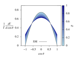
Figure 4: Normalized uni-angular distribution showing the effect of a scalar new physics contribution to $B\to P\ell^{-}f^{\textrm{\char 55}}$ where we have neglected the mass of the charged lepton $\ell=e,\mu$. This also shows the normalized uni-angular distribution showing the effect of a scalar new physics contribution to $B\to Kf_{1}^{\textrm{\char 51}}f_{2}^{\textrm{\char 55}}$ considering the $m_{1}=m_{2}$ case only.

From Eq. (26) it is clear that despite the scalar NP effect, the distribution is still symmetric under $\cos\theta\leftrightarrow-\cos\theta$, and solving for the number of events in the four segments of the Dalitz plot (equivalently the four $\cos\theta$ bins) we get,

$$\frac{N_{I}}{N_{II}}=\frac{5+8\epsilon_{0}}{11+8\epsilon_{0}}=\frac{N_{IV}}{N_{III}}.$$ (28)

It is easy to see that when $\epsilon=0$ we get back the SM prediction of Eq. (25) as expected.

Tensor type new physics:

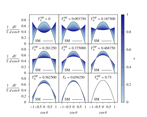
Figure 5: Normalized uni-angular distribution showing the effect of a tensor new physics contribution to $B\to P\ell^{-}f^{\textrm{\char 55}}$ where we have neglected the mass of the charged lepton $\ell=e,\mu$. These set of plots can also describe the effect of a vector new physics contribution to $B\to Kf_{1}^{\textrm{\char 51}}f_{2}^{\textrm{\char 55}}$ when the final fermions are equally massive.

Let us consider a tensor type of new physics possibility in which $F_{T_{1}}\neq 0$ and all other form factors are zero. In such a case we get,

$$C_{0}^{\textrm{NP}} =2m^{2}\left(s-m^{2}\right)\frac{\lambda\left(s,m_{B}^{2},m_{P}^{2}\right)}{s}\left|F_{T_{1}}\right|^{2},$$

$$C_{1}^{\textrm{NP}} =0,$$

$$C_{2}^{\textrm{NP}} =2\left(s-m^{2}\right)^{2}\frac{\lambda\left(s,m_{B}^{2},m_{P}^{2}\right)}{s}\left|F_{T_{1}}\right|^{2}.$$

It is easy to notice that in the limit $m\to 0$ we have $C_{0}\to 0$ but $C_{2}\not\to 0$. If we do the integration over $s$, then the normalized angular distribution is given by,

$$\frac{1}{\Gamma^{\textrm{NP}}}\frac{d\Gamma^{\textrm{NP}}}{d\cos\theta}=T_{0}^{\textrm{NP}}+T_{2}^{\textrm{NP}}\cos^{2}\theta,$$ (29)

where $T_{2}^{\textrm{NP}}=3\left(1/2-T_{0}^{\textrm{NP}}\right)$ and $T_{0}^{\textrm{NP}}=3c_{0}/\left(6c_{0}+2c_{2}\right)$ with

$$c_{j}=\int_{m^{2}}^{\left(m_{B}-m_{P}\right)^{2}}\frac{b\sqrt{s}\ C_{j}^{\textrm{NP}}}{128\pi^{3}m_{B}^{2}\left(m_{B}^{2}-m_{P}^{2}+s\right)}ds.$$

Thus in the limit $m\to 0$ we have $T_{0}=0$. If such a new physics were present, our observation of $B\to P\ell^{-}f^{\textrm{\char 55}}$ would have the following angular distribution,

$$\frac{d\Gamma}{d\cos\theta}=\Gamma^{\text{SM}}\left(\frac{3}{4}\sin^{2}\theta+\left(T_{0}^{\textrm{NP}}+3\left(\frac{1}{2}-T_{0}^{\textrm{NP}}\right)\cos^{2}\theta\right)\epsilon\right),$$ (30)

where $\epsilon=\Gamma^{\textrm{NP}}/\Gamma^{\textrm{SM}}$ is the NP parameter which can vary in the range $\left[0,1\right]$ denoting the possibility that the NP contribution can be as large as that of the SM, and $T_{0}^{\textrm{NP}}$ acts as a free parameter here which can vary in the range $\left[0,3/4\right]$ in which $d\Gamma^{\textrm{NP}}/d\cos\theta\geqslant 0$ for all values of $\cos\theta$. Doing integration over $\cos\theta$ we get $\Gamma=\Gamma^{\textrm{SM}}\left(1+\epsilon\right)=\Gamma^{\textrm{SM}}+\Gamma^{\textrm{NP}}$. This implies

$$\frac{1}{\Gamma}\frac{d\Gamma}{d\cos\theta}=\frac{3+4T_{0}^{\textrm{NP}}\epsilon-3\left(4T_{0}^{\textrm{NP}}\epsilon-2\epsilon+1\right)\cos^{2}\theta}{4\left(1+\epsilon\right)}.$$ (31)

This angular distribution is shown in Fig. 5 in which we have considered nine values of $T_{0}^{\textrm{NP}}$ and varied $\epsilon$ in the range $[0,1]$. It is clearly evident in Fig. 5 that $T_{0}^{\textrm{NP}}=3/4$ case is always indistinguishable from the SM case, as it should be. Just like the scalar-type new physics case, we observe that there are two values of $\cos\theta$ at which there is no difference between the SM prediction alone and the combination of SM and NP contributions. These two points can be easily computed by equating Eqs. (24) and (31), and then solving for $\cos\theta$ we once again find that,

$$\cos\theta=\pm 1/\sqrt{3}\approx\pm 0.57735,$$ (32)

which corresponds to the angle $\theta\approx 54.74^{\circ}$. At these two points in $\cos\theta$, the normalized uni-angular distribution always has the value $0.5$, even if there is some tensor new physics contributing to our process under consideration. It should be noted that these are also the same points where the scalar new physics contribution shows similar effect.

It is also easy to notice that the angular distribution as given in Eq. (31) is symmetric under $\cos\theta\leftrightarrow-\cos\theta$, and solving for the number of events in the four segments of the Dalitz plot (equivalently the four $\cos\theta$ bins) we get,

$$\frac{N_{I}}{N_{II}}=\frac{5+2\epsilon\left(7-6T_{0}^{\textrm{NP}}\right)}{11+2\epsilon\left(1+6T_{0}^{\textrm{NP}}\right)}=\frac{N_{IV}}{N_{III}}.$$ (33)

It is easy to see that when $\epsilon=0$ or $T_{0}^{\textrm{NP}}=3/4$ we get back the SM prediction of Eq. (25) as expected.

Finally we analyze new physics possibilities in the decays belonging to the GS2 category. Due to the very nature of the GS2 decay modes, the following discussion of NP effects presumes usage of advanced detector technology to get angular information.

V.3.2 New physics effects in the GS2 decay $B\to Kf_{1}^{\textrm{\char 51}}f_{2}^{\textrm{\char 55}}$

As mentioned before, the GS2 decay modes are originally part of S3, i.e. it is extremely difficult to get angular distribution for these cases unless we innovate on detector technology. Here we consider such a decay mode $B\to Kf_{1}^{\textrm{\char 51}}f_{2}^{\textrm{\char 55}}$ in which both $f_{1}$, $f_{2}$ are neutral fermions who have evaded, till now, all our attempts to detect them near their place of origin. But probably with displaced vertex detectors or some other advanced detector we could bring at least one of these fermions (say $f_{1}$) under the purview of experimental study and measure its 4-momentum or angular information. The missing fermion (which is $f_{2}$ in our example here) might have flied in a direction along which there is no detector coverage. To increase the sample size we should include $B\to Kf_{1}^{\textrm{\char 55}}f_{2}^{\textrm{\char 51}}$ events also, provided we know how to ascertain the particle or anti-particle nature of $f_{1}$ and $f_{2}$. To illustrate this point, let us consider the possibility $f_{1}f_{2}=\nu_{S}\overline{\nu}_{S}$. In a displaced vertex detector if we see $\pi^{+}\mu^{-}$ events, they can be attributed to the decay of $\nu_{S}$ and similarly $\pi^{-}\mu^{+}$ events would appear from the decay of $\overline{\nu}_{S}$. In this case, we can infer the angle $\theta$ by knowing the 4-momentum of either $f_{1}=\nu_{S}$ or $f_{2}=\overline{\nu}_{S}$ (see Fig. 2). If we find that both $f_{1}$ and $f_{2}$ leave behind their signature tracks in the detector (i.e. $f_{1}^{\textrm{\char 51}}f_{2}^{\textrm{\char 51}}$) it would be the most ideal situation. But as we have already stressed before, measuring 4-momenta of either of the fermions would suffice for our angular studies.

In the SM the only contribution to $B\to Kf_{1}^{\textrm{\char 51}}f_{2}^{\textrm{\char 55}}$ and $B\to Kf_{1}^{\textrm{\char 55}}f_{2}^{\textrm{\char 51}}$ would come from $B\to K\nu_{\ell}\overline{\nu}_{\ell}$ where as in the case of NP we have a number of possibilities that includes sterile neutrinos, dark matter particles, or some long lived particles in the final state, $f_{1}f_{2}=\nu_{\ell}\overline{\nu}_{S}$, $\nu_{S}\overline{\nu}_{\ell}$, $\nu_{S}\overline{\nu}_{S}$, $f^{\textrm{DM}}\bar{f}^{\textrm{DM}}$, $f_{1}^{\textrm{DM}}f_{2}^{\textrm{DM}}$, $f^{\textrm{LLP}}\bar{f}^{\textrm{LLP}}$, $f_{1}^{\textrm{LLP}}f_{2}^{\textrm{LLP}}$ etc. One can also consider non-standard neutrino interactions also contributing in these cases. To demonstrate our methodology, we shall analyze only a subset of these various NP possibilities in which $f_{1}$ and $f_{2}$ have the same mass, i.e. $m_{1}=m_{2}=m$ (say), as this greatly simplifies the calculation. As we shall illustrate below we can not only detect the presence of NP but ascertain whether it is of scalar type or vector type, for example, by analyzing the angular distribution.

Before, we go for new physics contributions, let us analyze the SM contribution $B\to K\nu_{\ell}\overline{\nu}_{\ell}$. Here only vector and axial-vector currents contributions, and $F_{A}^{\pm}=-F_{V}^{\pm}$. Also the neutrino and anti-neutrino are massless, i.e. $m_{1}=0=m_{2}$, which implies $a_{t}=a_{u}=\tfrac{1}{2}\left(m_{B}^{2}+m_{K}^{2}-s\right)$ and $b=\tfrac{1}{2}\sqrt{\lambda\left(s,m_{B}^{2},m_{K}^{2}\right)}$, where $m_{B}$ and $m_{K}$ denote the masses of $B$ and $K$ mesons respectively. Substituting these information in Eqs. (10) and in Eq. (7) we get,

$$\frac{d^{2}\Gamma^{\text{SM}}}{ds\,d\cos\theta}=\frac{b^{3}\sqrt{s}}{8\,\pi^{3}\,m_{B}^{2}\left(m_{B}^{2}-m_{K}^{2}+s\right)}\left|\left(F_{V}^{+}\right)_{\text{SM}}\right|^{2}\sin^{2}\theta.$$ (34)

Irrespective of the expression for $\left(F_{V}^{+}\right)_{\text{SM}}$, it can be easily shown that the normalized angular distribution is given by,

$$\frac{1}{\Gamma^{\text{SM}}}\frac{d\Gamma^{\text{SM}}}{d\cos\theta}=\frac{3}{4}\sin^{2}\theta,$$ (35)

which implies that $T_{0}=3/4=-T_{2}$, $T_{1}=0$. Following the same logic as the one given after Eq. (24), we find that the number of events in the different segments of the Dalitz plot (equivalently the number of events in the four distinct bins of $\cos\theta$) are related to one another by,

$$\frac{N_{I}}{N_{II}}=\frac{5}{11}=\frac{N_{IV}}{N_{III}}.$$ (36)

This sets the stage for us to explore (i) a scalar type and (ii) a vector type of NP possibility, with final fermions for which $m_{1}=m_{2}=m\neq 0$.

Scalar type new physics:

Once again we consider the simplest scalar type NP scenario, with $F_{S}\neq 0$, and other form factors being zero. This leads us to,

$$C_{0}^{\text{NP}}= 2\left(s-4m^{2}\right)\left|F_{S}\right|^{2},$$

$$C_{1}^{\text{NP}}= 0=C_{2}^{\text{NP}}.$$

In other words, there is no angular dependence at all here, i.e.

$$\frac{d^{2}\Gamma^{\text{NP}}}{ds\,d\cos\theta}=\frac{b\sqrt{s}}{64\,\pi^{3}\,m_{B}^{2}\left(m_{B}^{2}-m_{K}^{2}+s\right)}\left(s-4m^{2}\right)\left|F_{S}\right|^{2},$$ (37)

where $b=\left(\sqrt{\left(s-4m^{2}\right)}\,\sqrt{\lambda\left(s,m_{B}^{2},m_{K}^{2}\right)}\right)/(2\sqrt{s})$ and $4m^{2}\leqslant s\leqslant\left(m_{B}-m_{K}\right)^{2}$. If we do the integration over $s$, then for NP only the normalized angular distribution is given by,

$$\frac{1}{\Gamma^{\text{NP}}}\frac{d\Gamma^{\text{NP}}}{d\cos\theta}=\frac{1}{2}.$$

Assuming such a NP contributing in addition to the SM, the experimentally observed angular distribution can be written as,

$$\frac{d\Gamma}{d\cos\theta}=\Gamma^{\text{SM}}\left(\frac{3}{4}\sin^{2}\theta+\frac{1}{2}\epsilon_{0}\right),$$

where $\epsilon_{0}=\Gamma^{\text{NP}}/\Gamma^{\text{SM}}$ is the new physics parameter which can vary in the range $\left[0,1\right]$ if we assume the NP contribution to be as large as that from the SM. Doing integration over $\cos\theta$ we get, $\Gamma=\Gamma^{\text{SM}}\left(1+\epsilon_{0}\right)=\Gamma^{\text{SM}}+\Gamma^{\text{NP}}$. This implies

$$\frac{1}{\Gamma}\frac{d\Gamma}{d\cos\theta}=\frac{3\sin^{2}\theta+2\epsilon_{0}}{4\left(1+\epsilon_{0}\right)}.$$ (38)

Since Eq. (38) is identical to Eq. (26), the angular distribution for this case is also as shown in Fig. 4 where we have varied $\epsilon_{0}$ in the range $[0,1]$. Once again at two specific values of $\cos\theta$, namely $\cos\theta=\pm 1/\sqrt{3}\approx\pm 0.57735$ corresponding to the angle $\theta\approx 54.74^{\circ}$, there is no difference between the standard model prediction alone and the combination of standard model and scalar new physics contribution. At these two points in $\cos\theta$, the normalized uni-angular distribution always has the value $0.5$, even if there is some scalar new physics contributing to our process under consideration.

Since the angular distribution as shown in Eq. (38) is fully symmetric under $\cos\theta\leftrightarrow-\cos\theta$, the number of events in the four segments of the Dalitz plot (equivalently in the four $\cos\theta$ bins) satisfy the following relationship,

$$\frac{N_{I}}{N_{II}}=\frac{5+8\epsilon_{0}}{11+8\epsilon_{0}}=\frac{N_{IV}}{N_{III}}.$$ (39)

It is easy to see that $\epsilon_{0}=0$ gives the SM prediction of Eq. (36) as expected.

Vector type new physics:

Let us now discuss another new physics scenario, such as the case of a flavor-changing $Z^{\prime}$ or a dark photon $\gamma_{D}$ giving rise to the final pair of fermions $f_{1}f_{2}$. We assume that for this kind of new physics scenario, $F_{V}^{+}=F_{V}^{\text{NP}}\neq 0$ and other form factors are zero. For this kind of new physics we get,

$$C_{0}^{\text{NP}}= 2\left|F_{V}^{\text{NP}}\right|^{2}\lambda\left(s,m_{B}^{2},m_{K}^{2}\right),$$

$$C_{1}^{\text{NP}}= 0,$$

$$C_{2}^{\text{NP}}= -8b^{2}\left|F_{V}^{\text{NP}}\right|^{2},$$

where $b=\left(\sqrt{\left(s-4m^{2}\right)}\,\sqrt{\lambda\left(s,m_{B}^{2},m_{K}^{2}\right)}\right)/\left(2\sqrt{s}\right)$ and $4m^{2}\leqslant s\leqslant\left(m_{B}-m_{K}\right)^{2}$. The angular distribution for the NP alone contribution can, therefore, be written in terms of $T_{0}^{\textrm{NP}}$ and $T_{2}^{\textrm{NP}}$ which are directly proportional to $C_{0}^{\text{NP}}$ and $C_{2}^{\text{NP}}$ respectively. It would lead us to describe the complete angular distribution in terms of $T_{0}^{\text{NP}}$ and $\epsilon=\Gamma^{\textrm{NP}}/\Gamma^{SM}$ using Eq. (31) and the angular distribution would look like the one shown in Fig. 5. However, it is possible to describe the effects of NP on the angular distribution using a different set of parameters as well. For this we start a fresh with the angular distribution for the NP contribution alone, which in our case is given by

$$\frac{d^{2}\Gamma^{\text{NP}}}{ds\,d\cos\theta}=\frac{b\left|F_{V}^{\text{NP}}\right|^{2}\lambda\left(s,m_{B}^{2},m_{K}^{2}\right)\,\left(s\sin^{2}\theta+4m^{2}\cos^{2}\theta\right)}{64\,\pi^{3}\,m_{B}^{2}\left(m_{B}^{2}-m_{K}^{2}+s\right)\sqrt{s}}.$$

Doing integration over $\cos\theta$ we obtain,

$$\frac{d\Gamma^{\text{NP}}}{ds}=\frac{b\left|F_{V}^{\text{NP}}\right|^{2}\lambda\left(s,m_{B}^{2},m_{K}^{2}\right)}{64\,\pi^{3}\,m_{B}^{2}\left(m_{B}^{2}-m_{K}^{2}+s\right)\sqrt{s}}\left(\frac{4s+8m^{2}}{3}\right).$$

Therefore, the normalized uni-angular distribution is given by

$$\frac{1}{d\Gamma^{\text{NP}}/ds}\frac{d^{2}\Gamma^{\text{NP}}}{ds\,d\cos\theta}=\frac{3}{4}\left(\frac{s\sin^{2}\theta+4m^{2}\cos^{2}\theta}{s+2m^{2}}\right).$$ (40)

It is interesting to compare this with the standard model expression,

$$\frac{1}{d\Gamma^{\text{SM}}/ds}\frac{d^{2}\Gamma^{\text{SM}}}{ds\,d\cos\theta}=\frac{3}{4}\sin^{2}\theta.$$ (41)

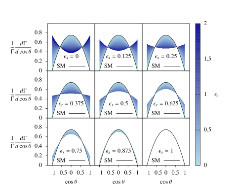
Figure 6: Normalized uni-angular distribution showing the effect of a vector new physics contribution to $B\to Kf_{1}^{\textrm{\char 51}}f_{2}^{\textrm{\char 55}}$.

Since the range for $s$ is different in the SM and the NP scenarios, we can not add Eqs. (40) and (41) directly. Carrying out the integration over $s$ we get,

$$\frac{d\Gamma^{\text{NP}}}{d\cos\theta}=\frac{3}{4}\Big{(}\mathcal{S}\sin^{2}\theta+\mathcal{C}\cos^{2}\theta\Big{)},$$

where

$$\mathcal{S} =\int_{4m^{2}}^{(m_{B}-m_{K})^{2}}\frac{d\Gamma^{\text{NP}}}{ds}\left(\frac{s}{s+2m^{2}}\right)ds,$$

$$\mathcal{C} =\int_{4m^{2}}^{(m_{B}-m_{K})^{2}}\frac{d\Gamma^{\text{NP}}}{ds}\left(\frac{4m^{2}}{s+2m^{2}}\right)ds.$$

Doing integration over $\cos\theta$ we get,

$$\Gamma^{\text{NP}}=\mathcal{S}+\mathcal{C}/2,$$

and hence

$$\frac{1}{\Gamma^{\text{NP}}}\frac{d\Gamma^{\text{NP}}}{d\cos\theta}=\frac{3\left(\mathcal{S}\sin^{2}\theta+\mathcal{C}\cos^{2}\theta\right)}{2(2\mathcal{S}+\mathcal{C})}.$$

For the SM contribution we know that

$$\frac{1}{\Gamma^{\text{SM}}}\frac{d\Gamma^{\text{SM}}}{d\cos\theta}=\frac{3}{4}\sin^{2}\theta.$$

Now the uni-angular distribution for the process $B\to Kf_{1}^{\textrm{\char 51}}f_{2}^{\textrm{\char 55}}$ is given by,

$$\frac{d\Gamma}{d\cos\theta}=\frac{3}{4}\Gamma^{\text{SM}}\left(\left(1+\epsilon_{s}\right)\sin^{2}\theta+\epsilon_{c}\cos^{2}\theta\right),$$

where $\epsilon_{s}=\mathcal{S}/\Gamma^{\text{SM}}$ and $\epsilon_{c}=\mathcal{C}/\Gamma^{\text{SM}}$, are the two parameters which describe the effect of vector type NP. It is easy to check that,

$$\Gamma=\frac{3}{4}\Gamma^{\text{SM}}\left(\frac{4}{3}\left(1+\epsilon_{s}\right)+\frac{2\epsilon_{c}}{3}\right)=\Gamma^{\text{SM}}+\Gamma^{\text{NP}}.$$

Therefore, the normalized angular distribution is given by,

$$\frac{1}{\Gamma}\frac{d\Gamma}{d\cos\theta}=\frac{3\left(1+\epsilon_{s}\right)\sin^{2}\theta+3\epsilon_{c}\cos^{2}\theta}{4\left(1+\epsilon_{s}\right)+2\epsilon_{c}}.$$ (42)

It is important to note that, if we consider the mass of the fermion $f$ to be zero, i.e. $m=0$, then $\epsilon_{c}=0$, since $\mathcal{C}=0$. In such a case the uni-angular distribution is given by,

$$\frac{1}{\Gamma}\frac{d\Gamma}{d\cos\theta}=\frac{3}{4}\sin^{2}\theta,\qquad\left(\text{here }\epsilon_{c}=0\right)$$

which is same as that of the SM case. This is plausible, as in the SM case also one has $m=0$ for the neutrino mass and only vector and axial-vector currents contribute.

Assuming that the NP contribution can be smaller than or as large as the SM contribution, i.e. $0\leqslant\Gamma^{\text{NP}}\leqslant\Gamma^{\text{SM}}$, we get

$$0\leqslant\epsilon_{s}+\epsilon_{c}/2\leqslant 1.$$

Thus $0\leqslant\epsilon_{s}\leqslant 1$ implies that $0\leqslant\epsilon_{c}\leqslant 2(1-\epsilon_{s})$.

In Fig. 6 we have considered nine values of $\epsilon_{s}$ and varied $\epsilon_{c}$ in the range $[0,2\left(1-\epsilon_{s}\right)]$, to obtain the uni-angular distribution. It is clearly evident in Fig. 6 that $\epsilon_{c}=0$ case is always indistinguishable from the SM case, as it should be. Just like the scalar-type new physics case, we observe that at $\cos\theta=\pm 1/\sqrt{3}\approx\pm 0.57735$, there is no difference between the SM prediction alone and the combination of SM and NP contributions.

It is also easy to notice that the angular distribution as given in Eq. (42) is symmetric under $\cos\theta\leftrightarrow-\cos\theta$, and solving for the number of events in the four segments of the Dalitz plot (equivalently the four $\cos\theta$ bins) we get,

$$\frac{N_{I}}{N_{II}}=\frac{5\left(1+\epsilon_{s}\right)+7\epsilon_{c}}{11\left(1+\epsilon_{s}\right)+\epsilon_{c}}=\frac{N_{IV}}{N_{III}}.$$ (43)

It is easy to see that when $\epsilon_{c}=0=\epsilon_{s}$ we get back the SM prediction of Eq. (36) as expected.

V.4 Discussion

It should be noted that our discussions on the types of NP contributions to the S2 and GS2 modes, specifically $B\to P\ell^{-}f^{\textrm{\char 55}}$ and $B\to Kf_{1}^{\textrm{\char 51}}f_{2}^{\textrm{\char 55}}$ respectively, has been fully general. There is no complications arising out of hadronic form factors since we have considered normalized angular distribution. It should be noted that our analysis also does not depend on how large or small the masses of the fermions $f,f_{1,2}$ are, as long as they are non-zero.

It is also very interesting to note that both the scalar and tensor type of NP for the $B\to P\ell^{-}f^{\textrm{\char 55}}$ decays and both the scalar and vector types of NP for the $B\to Kf_{1}^{\textrm{\char 51}}f_{2}^{\textrm{\char 55}}$ decays, exhibit similar behaviour at $\cos\theta=\pm 1/\sqrt{3}$. In order to know the real reason behind this we must do a very general analysis. Let us assume that the most general angular distribution for the processes $B\to P\ell^{-}f^{\textrm{\char 55}}$ and $B\to Kf_{1}^{\textrm{\char 51}}f_{2}^{\textrm{\char 55}}$ is given by Eq. (12). If we now equate this distribution to the SM prediction of Eq. (24) or Eq. (35), and solve for $\cos\theta$ after substituting Eq. (13) we find that,

$$\cos\theta=\frac{-c_{1}\pm\sqrt{c_{1}^{2}+3\left(c_{0}+c_{2}\right)^{2}}}{3\left(c_{0}+c_{2}\right)},$$ (44)

where the $c_{j}$’s (for $j=0,1,2$) are obtained from Eq. (14) with appropriate substitutions of masses and form factors. Thus Eq. (44) is the most general solution that we can get for the two specific values of $\cos\theta$. However, let us look at the specific case when $c_{1}=0$. Only in this situation do we get

$$\cos\theta=\pm 1/\sqrt{3}.$$ (45)

Now it is clear that since, in both the scalar and tensor type of NP considerations for the $B\to P\ell^{-}f^{\textrm{\char 55}}$ decays and in both the scalar and vector types of NP considerations for the $B\to Kf_{1}^{\textrm{\char 51}}f_{2}^{\textrm{\char 55}}$ decays, the angular distribution did not have any term directly proportional to $\cos\theta$ (i.e. $c_{1}=0$), we obtained the same $\cos\theta=\pm 1/\sqrt{3}$ result in both the cases. Therefore, if the observed normalized uni-angular distribution does not have the value $0.5$ at $\cos\theta=\pm 1/\sqrt{3}$, it implies that $c_{1}\neq 0$.

Another interesting aspect of the two specific NP contributions we have considered, is that from Figs. 4, 5 and 6 one can clearly see that the vector and tensor types of NP can accommodate a much larger variation in the angular distribution than the scalar type NP. However, there is also a certain part of the angular distribution for which both scalar and vector (or tensor) types of NP give identical results. This happens when

$$\epsilon_{0}=\frac{3\epsilon_{c}}{2\left(1+\epsilon_{s}-\epsilon_{c}\right)}=\frac{\epsilon\left(3-4T_{0}^{\textrm{NP}}\right)}{1-\epsilon\left(2-4T_{0}^{\textrm{NP}}\right)}.$$ (46)

In order for $\epsilon_{0}$ to vary in the range $[0,1]$ we find that (i) for $0\leqslant\epsilon_{s}\leqslant 1$ we have $0\leqslant\epsilon_{c}\leqslant 2\left(1+\epsilon_{s}\right)/5$ and (ii) for $0\leqslant\epsilon\leqslant 1$ we have $\frac{1}{2}\leqslant T_{0}^{\textrm{NP}}\leqslant\frac{3}{4}$. In these specific regions, therefore, it would not be possible to clearly distinguish whether scalar or vector or tensor type NP is contributing to our process under consideration. Nevertheless, our approach can be used to constraint these NP hypothesis without any hadronic uncertainties.

VI Conclusion

We have shown that all NP contributions to three-body semi-hadronic decays of the type $P_{i}\to P_{f}f_{1}f_{2}$, where $P_{i(f)}$ denotes appropriate initial (final) pseudo-scalar meson and $f_{1,2}$ are a pair of fermions, can be codified into the most general Lagrangian which gives rise to a very general angular distribution. The relevant NP information can be obtained by using various angular asymmetries, provided at least one of the final pair of fermions has some detectable signature, such as a displaced vertex, in the detector. Depending on the detection feasibility of the final fermions we have grouped the $P_{i}\to P_{f}f_{1}f_{2}$ decays into three distinct categories: (i) S1 where both $f_{1}$ and $f_{2}$ are detected, (ii) S2 where either $f_{1}$ or $f_{2}$ gets detected, and (ii) S3 where neither $f_{1}$ nor $f_{2}$ gets detected. We consider the possibility that with advancement in detector technology S3 decays could, in future, be grouped under S2 category. We analyze some specific NP scenarios in each of these categories to illustrate how NP affects the angular distribution. Specifically we have analyzed (a) lepton-flavor violating S1 decay $B\to P\ell^{-}\ell^{\prime+}$ (with $P=\pi,K,D$ and $\ell,\ell^{\prime}=e,\mu,\tau$) showing angular signatures of all generic NP possibilities, (b) S2 decays of the type $B\to P\ell^{-}f$ (where $f$ is not detected in the laboratory) showing the effect of a scalar type and a tensor type NP on the angular distribution, and finally (c) S3 decays (more correctly generalized S2 decays) of the type $B\to Kf\bar{f}$ (where either $f$ or $\bar{f}$ gets detected in an advanced detector) showing the effects of a scalar type and a vector type NP on the angular distribution. The effects on the angular distribution can be easily estimated from Dalitz plot asymmetries. The signatures of NP in angular distribution are distinct once the process is chosen carefully. Moreover, as shown in our examples it can be possible to do the identification and quantification of NP effects without worrying about hadronic uncertainties. We are optimistic that our methodology can be put to use in LHCb, Belle II in the study of appropriate $B$ meson decays furthering our search for NP.

- (1) R. Aaij et al. [LHCb Collaboration], JHEP 1708, 055 (2017); R. Aaij et al. [LHCb Collaboration], JHEP 1602, 104 (2016); R. Aaij et al. [LHCb Collaboration], Phys. Rev. Lett. 113, 151601 (2014).
- (2) R. Aaij et al. [LHCb Collaboration], JHEP 1509, 179 (2015).
- (3) A. Abdesselam et al. [Belle Collaboration], arXiv:1603.06711 [hep-ex]; R. Aaij et al. [LHCb Collaboration], Phys. Rev. Lett. 115, no. 11, 111803 (2015), Erratum: [Phys. Rev. Lett. 115, no. 15, 159901 (2015)]; M. Huschle et al. [Belle Collaboration], Phys. Rev. D 92, no. 7, 072014 (2015); J. P. Lees et al. [BaBar Collaboration], Phys. Rev. D 88, no. 7, 072012 (2013).
- (4) R. Aaij et al. [LHCb Collaboration], Phys. Rev. Lett. 120, no. 12, 121801 (2018).
- (5) C. S. Kim and D. Sahoo, Eur. Phys. J. C 77, no. 9, 582 (2017).
- (6) N. Isgur and M. B. Wise, Phys. Lett. B 237, 527 (1990); M. Neubert, Phys. Rept. 245, 259 (1994); A. V. Manohar and M. B. Wise, Camb. Monogr. Part. Phys. Nucl. Phys. Cosmol. 10, 1 (2000); N. Uraltsev, In Shifman, M. (ed.): At the frontier of particle physics, vol. 3 1577-1670 (2001); A. G. Grozin, Springer Tracts Mod. Phys. 201, 1 (2004).
- (7) J. E. Mandula, M. C. Ogilvie, Nucl. Phys. Proc. Suppl. 34, 480 (1994); T. Bhattacharya and R. Gupta, Nucl. Phys. Proc. Suppl. 47, 481 (1996); J. M. Flynn, In ‘Campagnari, C. (ed.): Santa Barbara 1997, Heavy flavor physics,’ p.40-51, hep-lat/9710080; J. M. Flynn and C. T. Sachrajda, Adv. Ser. Direct. High Energy Phys. 15, 402 (1998); S. Hashimoto, A. X. El-Khadra, A. S. Kronfeld, P. B. Mackenzie, S. M. Ryan and J. N. Simone, Phys. Rev. D 61, 014502 (1999); S. Hashimoto, A. S. Kronfeld, P. B. Mackenzie, S. M. Ryan and J. N. Simone, Phys. Rev. D 66, 014503 (2002); G. M. de Divitiis, E. Molinaro, R. Petronzio and N. Tantalo, Phys. Lett. B 655, 45 (2007); G. M. de Divitiis, R. Petronzio and N. Tantalo, JHEP 0710, 062 (2007).
- (8) P. Ball and R. Zwicky, Phys. Rev. D 71, 014015 (2005); A. Khodjamirian, T. Mannel and N. Offen, Phys. Rev. D 75, 054013 (2007); S. Faller, A. Khodjamirian, C. Klein and T. Mannel, Eur. Phys. J. C 60, 603 (2009); A. Khodjamirian, C. Klein, T. Mannel and N. Offen, Phys. Rev. D 80, 114005 (2009); A. Khodjamirian, T. Mannel, N. Offen and Y.-M. Wang, Phys. Rev. D 83, 094031 (2011); A. Bharucha, JHEP 1205, 092 (2012); Y. M. Wang and Y. L. Shen, Nucl. Phys. B 898, 563 (2015); N. Gubernari, A. Kokulu and D. van Dyk, arXiv:1811.00983 [hep-ph].
- (9) M. A. Ivanov, J. G. Korner, S. G. Kovalenko, P. Santorelli and G. G. Saidullaeva, Phys. Rev. D 85, 034004 (2012); M. A. Ivanov, J. G. Körner and C. T. Tran, Phys. Rev. D 92, no. 11, 114022 (2015); M. A. Ivanov and C. T. Tran, Phys. Rev. D 92, no. 7, 074030 (2015); M. A. Ivanov, J. G. Körner and C. T. Tran, Phys. Rev. D 94, no. 9, 094028 (2016).
- (10) J. Gratrex, M. Hopfer and R. Zwicky, Phys. Rev. D 93, no. 5, 054008 (2016).
- (11) F. Beaujean, M. Chrząszcz, N. Serra and D. van Dyk, Phys. Rev. D 91, no. 11, 114012 (2015).
- (12) A. Ali, P. Ball, L. T. Handoko and G. Hiller, Phys. Rev. D 61, 074024 (2000); C. Bobeth, T. Ewerth, F. Kruger and J. Urban, Phys. Rev. D 64, 074014 (2001); C. Bobeth, G. Hiller and G. Piranishvili, JHEP 0712, 040 (2007).
- (13) B. Aubert et al. [BaBar Collaboration], Phys. Rev. D 73, 092001 (2006); R. Aaij et al. [LHCb Collaboration], JHEP 1405, 082 (2014); D. Wang [CMS Collaboration], PoS BEAUTY 2018, 045 (2018); A. M. Sirunyan et al. [CMS Collaboration], arXiv:1806.00636 [hep-ex].
- (14) G. Cottin, J. C. Helo and M. Hirsch, Phys. Rev. D 97, no. 5, 055025 (2018); G. Cottin, JHEP 1803, 137 (2018); S. Antusch, E. Cazzato and O. Fischer, Phys. Lett. B 774, 114 (2017); D. Dercks, J. De Vries, H. K. Dreiner and Z. S. Wang, arXiv:1810.03617 [hep-ph]; C. Dib and C. S. Kim, Phys. Rev. D 89, no. 7, 077301 (2014).
- (15) G. Aad et al. [ATLAS Collaboration], JHEP 1411, 088 (2014); V. Khachatryan et al. [CMS Collaboration], Phys. Rev. D 91, no. 1, 012007 (2015); The ATLAS collaboration [ATLAS Collaboration], ATLAS-CONF-2017-026; R. Aaij et al. [LHCb Collaboration], Eur. Phys. J. C 77, no. 4, 224 (2017); J. P. Chou, D. Curtin and H. J. Lubatti, Phys. Lett. B 767, 29 (2017); C. Alpigiani [MATHUSLA Collaboration], PoS ALPS 2018, 033 (2018); V. V. Gligorov, S. Knapen, M. Papucci and D. J. Robinson, Phys. Rev. D 97, no. 1, 015023 (2018); J. L. Feng, I. Galon, F. Kling and S. Trojanowski, Phys. Rev. D 97, no. 3, 035001 (2018).
- (16) C. S. Kim, S. C. Park, K. Wang and G. Zhu, Phys. Rev. D 81, 054004 (2010).