Multiple-Instance Learning
by Boosting Infinitely Many Shapelet-based Classifiers

Abstract

We propose a new formulation of Multiple-Instance Learning (MIL). In typical MIL settings, a unit of data is given as a set of instances called a bag and the goal is to find a good classifier of bags based on similarity from a single or finitely many “shapelets” (or patterns), where the similarity of the bag from a shapelet is the maximum similarity of instances in the bag. Classifiers based on a single shapelet are not sufficiently strong for certain applications. Additionally, previous work with multiple shapelets has heuristically chosen some of the instances as shapelets with no theoretical guarantee of its generalization ability. Our formulation provides a richer class of the final classifiers based on infinitely many shapelets. We provide an efficient algorithm for the new formulation, in addition to generalization bound. Our empirical study demonstrates that our approach is effective not only for MIL tasks but also for Shapelet Learning for time-series classification.

1 Introduction

Multiple-Instance Learning (MIL) is a fundamental framework of supervised learning with a wide range of applications such as prediction of molecule activity, image classification, and so on. Since the notion of MIL was first proposed by Dietterich et al. (1997), MIL has been extensively studied both in theoretical and practical aspects (Gärtner et al., 2002; Andrews et al., 2003; Sabato and Tishby, 2012; Zhang et al., 2013; Doran and Ray, 2014; Carbonneau et al., 2018).

A standard MIL setting is described as follows: A learner receives sets $B_{1},B_{2},\ldots,B_{m}$ called bags, each of which contains multiple instances. In the training phase, each bag is labeled but instances are not labeled individually. The goal of the learner is to obtain a hypothesis that predicts the labels of unseen bags correctly. One of the most common hypotheses used in practice has the following form:

$$h_{\bf u}(B)=\max_{x\in B}\left\langle{\bf u},\Phi(x)\right\rangle,$$ (1)

where $\Phi$ is a feature map and ${\bf u}$ is a feature vector which we call a shapelet. In many applications, ${\bf u}$ is interpreted as a particular “pattern” in the feature space and the inner product as the similarity of $\Phi(x)$ from ${\bf u}$. Note that we use the term “shapelets” by following the terminology of Shapelet Learning, which is a framework for time-series classification, although it is often called “concepts” in the literature of MIL. Intuitively, this hypothesis evaluates a given bag by the maximum similarity of the instances in the bag from the shapelet ${\bf u}$. Multiple-Instance Support Vector Machine (MI-SVM) proposed by Andrews et al. (2003) is a widely used algorithm that uses this hypothesis class and learns ${\bf u}$. It is well-known that MIL algorithms using this hypothesis class practically perform well for various multiple-instance datasets. Moreover, a generalization error bound of the hypothesis class is given by Sabato and Tishby (2012).

However, in some domains such as image recognition and document classification, it is said that the hypothesis class of (1) is not effective enough (see, e.g., Chen et al., 2006). To employ MIL on such domains more effectively, Chen et al. (2006) proposes to use a convex combination of various shapelets ${\bf u}$ in a finite set $U=\{\Phi(z)\mid z\in\bigcup_{i=1}^{n}B_{i}\}$, which is defined based on all instances that appear in the training sample,

$$g(B)=\sum_{{\bf u}\in U}w_{\bf u}\max_{x\in B}\left\langle{\bf u},\Phi(x)\right\rangle,$$ (2)

where ${\bf w}$ is a probability vector over $U$. They demonstrate that this hypothesis with the Gaussian kernel performs well in image recognition. However, no theoretical justification is known for the hypothesis class of type (2) with the finite set $U$ made from the empirical bags. By contrast, for sets $U$ of infinitely many shapelets ${\bf u}$ with bounded norm, generalization bounds of Sabato and Tishby (2012) are applicable as well to the hypothesis class (2), but the result of Sabato and Tishby (2012) does not provide a practical formulation such as MI-SVM.

1.1 Our Contributions

In this paper, we propose an MIL formulation with the hypothesis class (2) for sets $U$ of infinitely many shapelets. More precisely, we formulate a $1$-norm regularized soft margin maximization problem to obtain linear combinations of shapelet-based hypotheses.

Then, we design an algorithm based on Linear Programming Boosting (LPBoost, Demiriz et al., 2002) that solves the soft margin optimization problem via a column generation approach. Although the sub-problems (weak learning problem) become optimization problems over an infinite-dimensional space, we can show that an analogue of the representer theorem holds on it and allows us to reduce it to a non-convex optimization problem (difference of convex program, DC-program for short) over a finite-dimensional space. While it is difficult to solve the sub-problems exactly due to non-convexity, various techniques (e.g., Tao and Souad, 1988; Yu and Joachims, 2009) are investigated for DC programs and we can find good approximate solutions efficiently for many cases in practice.

Furthermore, we prove a generalization error bound of hypothesis class (2) with infinitely large sets $U$. In general, our bound is incomparable with those of Sabato and Tishby (2012), but ours has better rate in terms of the sample size $m$.

We introduce an important application of our result, shapelet learning for time-series classification (we show details later). In fact, in time-series domain, most shapelet learning algorithms have been designed heuristically. As a result, our proposed algorithm becomes the first algorithm for shapelet learning in time-series classification that guarantees the theoretical generalization performance.

Finally, the experimental results show that our approach performs favorably with a baseline for shapelet-based time-series classification tasks and outperforms baselines for several MIL tasks.

1.2 Comparison to Related Work

There are many MIL algorithms with hypothesis classes which are different from (1) or (2). (e.g., Gärtner et al., 2002; Zhang et al., 2006; Chen et al., 2006). Many of them adopt different approaches for the bag-labeling hypothesis from shapelet-based classifiers (e.g., Zhang et al. (2006) used a Noisy-OR based hypothesis and Gärtner et al. (2002) proposed a new kernel called a set kernel).

Sabato and Tishby (2012) proved generalization bounds of hypotheses classes for MIL including those of  (1) and (2) with infinitely large sets $U$. They also proved the PAC-learnability of the class (1) using the boosting approach under some technical assumptions. Their boosting approach is different from our work in that they assume that labels are consistent with some hypothesis of the form (1), while we consider arbitrary distributions over bags and labels.

It is known that other boosting-based methods achieve successful results for several MIL tasks (Auer and Ortner, 2004; Andrews and Hofmann, 2004; Zhang et al., 2006). They use different hypothesis classes than ours under different assumptions.

1.3 Connection between MIL and Shapelet Learning for Time Series Classification

Here we briefly mention that MIL with type (2) hypotheses is closely related to Shapelet Learning (SL), which is a framework for time-series classification and has been extensively studied by (Ye and Keogh, 2009; Keogh and Rakthanmanon, 2013; Hills et al., 2014; Grabocka et al., 2014) in parallel to MIL. SL is a notion of learning with a particular method of feature extraction, which is defined by a finite set $M\subseteq\mathbb{R}^{\ell}$ of real-valued “short” sequences called shapelets and a similarity measure (not necessarily a Mercer kernel) $K:\mathbb{R}^{\ell}\times\mathbb{R}^{\ell}\to\mathbb{R}$ in the following way. A time series ${\boldsymbol{\tau}}=(\tau[1],\dots,\tau[L])\in\mathbb{R}^{L}$ can be identified with a bag $B_{\boldsymbol{\tau}}=\{(\tau[j],\ldots,\tau[j+\ell-1])\mid 1\leq j\leq L-\ell+1\}$ consisting of all subsequences of ${\boldsymbol{\tau}}$ of length $\ell$. Then, the feature of ${\boldsymbol{\tau}}$ is a vector $\left(\max_{{\bf x}\in B_{\boldsymbol{\tau}}}K({\bf z},{\bf x})\right)_{{\bf z}\in M}$ of a fixed dimension $|M|$ regardless of the length $L$ of the time series ${\boldsymbol{\tau}}$. When we employ a linear classifier on top of the features, we obtain a hypothesis of the form

$$g({\boldsymbol{\tau}})=\sum_{{\bf z}\in M}w_{\bf z}\max_{{\bf x}\in B_{\tau}}K({\bf z},{\bf x}),$$ (3)

which is essentially the same form as (2), except that finding good shapelets $M$ is a part of the learning task, as well as to finding good weight vector ${\bf w}$. This is one of the most successful approach of SL (Hills et al., 2014; Grabocka et al., 2014, 2015; Renard et al., 2015; Hou et al., 2016), where a typical choice of $K$ is $K({\bf z},{\bf x})=-\|{\bf z}-{\bf x}\|_{2}$. However, almost all existing methods heuristically choose shapelets $M$ and have no theoretical guarantee on how good the choice of $M$ is.

Note also that in the SL framework, each ${\bf z}\in M$ is called a shapelet, while in this paper, we assume that $K$ is a kernel $K(z,x)=\langle\Phi(z),\Phi(x)\rangle$ and any ${\bf u}$ (not necessarily $\Phi(z)$ for some $z$) in the Hilbert space is called a shapelet.

Curiously, despite MIL and SL share similar motivations and hypotheses, the relationship between MIL and SL has not yet been pointed out. From the shapelet-perspective in MIL, the hypothesis (1) is regarded as a “single shapelet”-based hypothesis, and the hypothesis (2) is regarded as “multiple shapelet”-based hypothesis. We refer to a linear combination of maximum similarities based on shapelets such as (2) and (3) as shapelet-based classifiers.

2 Preliminaries

Let $\mathcal{X}$ be an instance space. A bag $B$ is a finite set of instances chosen from $\mathcal{X}$. The learner receives a sequence of labeled bags $S=((B_{1},y_{1}),\ldots,(B_{m},y_{m}))\in(2^{\mathcal{X}}\times\{-1,1\})^{m}$ called a sample, where each labeled bag is independently drawn according to some unknown distribution $D$ over $2^{\mathcal{X}}\times\{-1,1\}$. Let $P_{S}$ denote the set of all instances that appear in the sample $S$. That is, $P_{S}=\bigcup_{i=1}^{m}B_{i}$. Let $K$ be a kernel over $\mathcal{X}$, which is used to measure the similarity between instances, and let $\Phi:\mathcal{X}\to\mathbb{H}$ denote a feature map associated with the kernel $K$ for a Hilbert space $\mathbb{H}$, that is, $K(z,z^{\prime})=\langle\Phi(z),\Phi(z^{\prime})\rangle$ for instances $z,z^{\prime}\in\mathcal{X}$, where $\langle\cdot,\cdot\rangle$ denotes the inner product over $\mathbb{H}$. The norm induced by the inner product is denoted by $\|\cdot\|_{\mathbb{H}}$ defined as $\|{\bf u}\|_{\mathbb{H}}=\sqrt{\langle{\bf u},{\bf u}\rangle}$ for ${\bf u}\in\mathbb{H}$.

For each ${\bf u}\in\mathbb{H}$ which we call a shapelet, we define a shapelet-based classifier denoted by $h_{{\bf u}}$, as the function that maps a given bag $B$ to the maximum of the similarity scores between shapelet ${\bf u}$ and $\Phi(x)$ over all instances $x$ in $B$. More specifically,

$$h_{{\bf u}}(B)=\max_{x\in B}\left\langle{\bf u},\Phi(x)\right\rangle.$$

For a set $U\subseteq\mathbb{H}$, we define the class of shapelet-based classifiers as

$$H_{U}=\left\{h_{{\bf u}}\mid{\bf u}\in U\right\}$$

and let $\mathrm{conv}(H_{U})$ denote the set of convex combinations of shapelet-based classifiers in $H_{U}$. More precisely,

$$\mathrm{conv}(H_{U})= \left\{\int_{{\bf u}\in U}w_{\bf u}h_{\bf u}d{\bf u}\mid\text{$w_{\bf u}$ is a density over $U$}\right\}$$

$$= \left\{\sum_{{\bf u}\in U^{\prime}}w_{\bf u}h_{\bf u}\mid\forall{\bf u}\in U^{\prime},w_{\bf u}\geq 0,\right.$$

$$\left.\sum_{{\bf u}\in U^{\prime}}w_{\bf u}=1,\text{$U^{\prime}\subseteq U$ is a finite support}\right\}.$$

The goal of the learner is to find a hypothesis $g\in\mathrm{conv}(H_{U})$, so that its generalization error $\mathcal{E}_{D}(g)=\Pr_{(B,y)\sim D}[\mathrm{sign}(g(B))\neq y]$ is small. Note that since the final hypothesis $\mathrm{sign}\circ g$ is invariant to any scaling of $g$, we assume without loss of generality that

$$U=\{{\bf u}\in\mathbb{H}\mid\|{\bf u}\|_{\mathbb{H}}\leq 1\}.$$

Let $\mathcal{E}_{\rho}(g)$ denote the empirical margin loss of $g$ over $S$, that is, $\mathcal{E}_{\rho}(g)=|\{i\mid y_{i}g(B_{i})<\rho\}|/m$.

3 Optimization Problem Formulation

In this paper we formulate the problem as soft margin maximization with $1$-norm regularization, which ensures a generalization bound for the final hypothesis (see, e.g., Demiriz et al., 2002). Specifically, the problem is formulated as a linear programming problem (over infinitely many variables) as follows:

$$\max\limits_{\rho,w,\boldsymbol{\xi}}\; \rho-\frac{1}{\nu m}\sum_{i=1}^{m}\xi_{i}$$ (4)

sub.to $$\int_{{\bf u}\in U}y_{i}w_{{\bf u}}h_{\bf u}(B_{i})d{\bf u}\geq\rho-\xi_{i}\wedge\xi_{i}\geq 0,~{}i\in[m],$$

$$\int_{{\bf u}\in U}w_{{\bf u}}d{\bf u}=1,w_{\bf u}\geq 0,~{}\rho\in\mathbb{R},$$

where $\nu\in[0,1]$ is a parameter. To avoid the integral over the Hilbert space, it is convenient to consider the dual form:

$$\min\limits_{\gamma,{\bf d}}\; \gamma$$ (5)

sub.to $$\sum_{i=1}^{m}y_{i}d_{i}h_{\bf u}(B_{i})\leq\gamma,\;{\bf u}\in U,$$

$$0\leq d_{i}\leq 1/(\nu m),\;i\in[m],$$

$$\sum_{i=1}^{m}d_{i}=1,~{}\gamma\in\mathbb{R}.$$

The dual problem is categorized as a semi-infinite program (SIP) because it contains infinitely many constraints. Note that the duality gap is zero because the problem (5) is linear and the optimum is finite (Theorem 2.2 of Shapiro, 2009). We employ column generation to solve the dual problem: solve (5) for a finite subset $U^{\prime}\subseteq U$, find ${\bf u}$ to which the corresponding constraint is maximally violated by the current solution (column generation part), and repeat the procedure with $U^{\prime}=U^{\prime}\cup\{{\bf u}\}$ until a certain stopping criterion is met. In particular, we use LPBoost (Demiriz et al., 2002), a well-known and practically fast algorithm of column generation. Since the solution ${\bf w}$ is expected to be sparse due to the 1-norm regularization, the number of iterations is expected to be small.

Following the terminology of boosting, we refer to the column generation part as weak learning. In our case, weak learning is formulated as the following optimization problem:

$$\max_{{\bf u}\in\mathbb{H}}\;\sum_{i=1}^{m}y_{i}d_{i}\max_{x\in B_{i}}\left\langle{\bf u},\Phi\left(x\right)\right\rangle\;\text{sub.to}\;\|{\bf u}\|_{\mathbb{H}}^{2}\leq 1.$$ (6)

Thus, we need to design a weak learner for solving (6) for a given sample weighted by ${\bf d}$. It seems to be impossible to solve it directly because we only have access to $U$ through the associated kernel. Fortunately, we prove a version of representer theorem given below, which makes (6) tractable.

Theorem 1 (Representer Theorem)

The solution ${\bf u}^{*}$ of (6) can be written as ${\bf u}^{*}=\sum_{z\in P_{S}}\alpha_{z}\Phi(z)$ for some real numbers $\alpha_{z}$.

Our theorem can be derived from an application of the standard representer theorem (see, e.g., Mohri et al., 2012). Intuitively, we prove the theorem by decomposing the optimization problem (6) into a number of sub-problems, so that the standard representer theorem can be applied to each of the sub-problems. The detail of the proof is given in the supplementary materials. Note that Theorem 1 gives justification to the simple heuristics in the literature: choosing the shapelets extracted from $P_{S}$.

Theorem 1 says that the weak learning problem can be rewritten as the following tractable form:

OP 1: Weak Learning Problem

$$\min_{\boldsymbol{\alpha}}\; -\sum_{i=1}^{m}{d}_{i}y_{i}\max_{x\in B_{i}}\sum_{z\in P_{S}}\alpha_{z}K\left(z,x\right)$$

sub.to $$\sum_{z\in P_{S}}\sum_{v\in P_{S}}\alpha_{z}\alpha_{v}K\left(z,v\right)\leq 1.$$

Unlike the primal solution ${\bf w}$, the dual solution $\boldsymbol{\alpha}$ is not expected to be sparse. In order to obtain a more interpretable hypothesis, we propose another formulation of weak learning where 1-norm regularization is imposed on $\boldsymbol{\alpha}$, so that a sparse solution of $\boldsymbol{\alpha}$ will be obtained. In other words, instead of $U$, we consider the feasible set $\hat{U}=\left\{\sum_{z\in P_{S}}\alpha_{z}\Phi(z):\|\boldsymbol{\alpha}\|_{1}\leq 1\right\}$, where $\|\boldsymbol{\alpha}\|_{1}$ is the 1-norm of $\boldsymbol{\alpha}$.

OP 2: Sparse Weak Learning Problem

$$\min_{\boldsymbol{\alpha}}\; -\sum_{i=1}^{m}{d}_{i}y_{i}\max_{x\in B_{i}}\sum_{z\in P_{S}}\alpha_{z}K\left(z,x\right)$$

sub.to $$\|\boldsymbol{\alpha}\|_{1}\leq 1$$

Note that when running LPBoost with a weak learner for OP 3, we obtain a final hypothesis that has the same form of generalization bound as the one stated in Theorem 2, which is of a final hypothesis obtained when used with a weak learner for OP 3. To see this, consider a feasible space $\hat{U}_{\Lambda}=\left\{\sum_{z\in P_{S}}\alpha_{z}\Phi(z):\|\boldsymbol{\alpha}\|_{1}\leq\Lambda\right\}$ for a sufficiently small $\Lambda>0$, so that $\hat{U}_{\Lambda}\subseteq U$. Then since $H_{\hat{U}_{\Lambda}}\subseteq H_{U}$, a generalization bound for $H_{U}$ also applies to $H_{\hat{U}_{\Lambda}}$. On the other hand, since the final hypothesis $\mathrm{sign}\circ g$ for $g\in\mathrm{conv}(H_{\hat{U}_{\Lambda}})$ is invariant to the scaling factor $\Lambda$, the generalization ability is independent of $\Lambda$.

4 Algorithms

For completeness, we present the pseudo code of LPBoost in Algorithm 1.

For the rest of this section, we describe our algorithms for the weak learners. For simplicity, we denote by ${\mathbf{k}}_{x}\in\mathbb{R}^{P_{S}}$ a vector given by $k_{x,z}=K(z,x)$ for every $z\in P_{S}$. Then, the objective function of OP 3 (and OP 3) can be rewritten as

$$\sum_{i:y_{i}=-1}d_{i}\max_{x\in B_{i}}{\mathbf{k}}_{x}^{T}\boldsymbol{\alpha}-\sum_{i:y_{i}=1}d_{i}\max_{x\in B_{i}}{\mathbf{k}}_{x}^{T}\boldsymbol{\alpha},$$

which can be seen as a difference $F-G$ of two convex functions $F$ and $G$ of $\boldsymbol{\alpha}$. Therefore, the weak learning problems are DC programs and thus we can use DC algorithm (Tao and Souad, 1988; Yu and Joachims, 2009) to find an $\epsilon$-approximation of a local optimum. We employ a standard DC algorithm. That is, for each iteration $t$, we linearize the concave term $G$ with $\nabla_{\boldsymbol{\alpha}}G(\boldsymbol{\alpha}_{t})^{T}\boldsymbol{\alpha}$ at the current solution $\boldsymbol{\alpha}_{t}$, which is $\sum_{i:y_{i}=1}d_{i}{\mathbf{k}}_{x_{i}}^{T}\boldsymbol{\alpha}$ with $x_{i}=\arg\max_{x\in B_{i}}{\mathbf{k}}_{x}^{T}\boldsymbol{\alpha}$ in our case, and then update the solution to $\boldsymbol{\alpha}_{t+1}$ by solving the resultant convex optimization problem $\textsf{OP}^{\prime}_{t}$.

In addition, the problems $\textsf{OP}^{\prime}_{t}$ for OP 3 and OP 3 are reformulated as a second-order cone programming (SOCP) problem and an LP problem, respectively, and thus both problems can be efficiently solved. To this end, we introduce new variables $\lambda_{i}$ for all negative bags $B_{i}$ with $y_{i}=-1$ which represent the factors $\max_{x\in B_{i}}{\mathbf{k}}_{x}^{T}\boldsymbol{\alpha}$. Then we obtain the equivalent problem to $\textsf{OP}^{\prime}_{t}$ for OP 3 as follows:

$$\min_{\boldsymbol{\alpha},\boldsymbol{\lambda}}\; \sum_{i:y_{i}=-1}d_{i}\lambda_{i}-\sum_{i:y_{i}=1}d_{i}\max_{x\in B_{i}}{\mathbf{k}}_{x_{i}}^{T}\boldsymbol{\alpha}$$ (7)

sub.to $${\mathbf{k}}_{x}^{T}\boldsymbol{\alpha}\leq\lambda_{i}~{}(\forall i:y_{i}=-1,\forall x\in B_{i}),$$

$$\sum_{z\in P_{S}}\sum_{v\in P_{S}}\alpha_{z}\alpha_{v}K\left(z,v\right)\leq 1.$$

It is well known that this is an SOCP problem. Moreover, it is clear that $\textsf{OP}^{\prime}_{t}$ for OP 3 can be formulated as an LP problem. We describe the algorithm for OP 3 in Algorithm 2.

Algorithm 1 LPBoost using WeakLearn

Inputs:

      $S$, kernel $K$, $\nu\in(0,1]$, $\epsilon>0$

Initialize:

      ${\bf d}_{0}\leftarrow(\frac{1}{m},\ldots,\frac{1}{m}),\gamma=0$

for  $t=1,\dots$ do

     $h_{t}\leftarrow$ Run WeakLearn($S$, $K$, ${\bf d}_{t-1}$, $\epsilon$)

     if $\sum_{i=1}^{m}y_{i}d_{i}h_{t}(B_{i})\leq\gamma$ then

         $t=t-1$, break

     end if

$$(\gamma,{\bf d}_{t})\leftarrow\arg\min\limits_{\gamma,{\bf d}}\;\gamma$$

$$\text{sub.to}~{}~{}\sum_{i=1}^{m}y_{i}d_{i}h_{j}(B_{i})\leq\gamma~{}~{}(j=1,\ldots,t),~{}~{}$$

$$0\leq d_{i}\leq 1/\nu m~{}~{}(i\in[m]),\sum_{i=1}^{m}d_{i}=1,~{}\gamma\in\mathbb{R}.$$

end for

${\bf w}\leftarrow$ Lagrangian multipliers of the last solution

$g\leftarrow\sum_{j=1}^{t}w_{j}h_{j}$

return $\mathrm{sign}(g)$

Algorithm 2 WeakLearn using the DC Algorithm

Inputs:

      $S$, $K$, ${\bf d}$, $\epsilon$ (convergence parameter)

Initialize:

      $\boldsymbol{\alpha}_{0}\in\mathbb{R}^{|P_{S}|}$, $f_{0}\leftarrow\infty$

for $t=1,\dots$ do

     for $\forall k:y_{k}=+1$ do

         $\displaystyle x^{*}_{k}\leftarrow\arg\max_{x\in B_{k}}\sum_{z\in P_{S}}d_{k}\alpha_{z}K\left(z,x\right)$

     end for

      $\displaystyle f\leftarrow\min_{\boldsymbol{\alpha},\boldsymbol{\lambda}}\;$ $\displaystyle-\sum_{k:y_{k}=+1}{d}_{k}\sum_{z\in P_{S}}\alpha_{z}K\left(z,x_{k}^{*}\right)$ $\displaystyle+\sum_{r:y_{r}=-1}{d}_{r}\lambda_{r}$ (8) sub.to $\displaystyle\sum_{z\in P_{S}}\alpha_{z}K\left(z,x\right)\leq\lambda_{r}$ $\displaystyle~{}(\forall r:y_{r}=-1,\forall x\in B_{r}),$ $\displaystyle\sum_{z\in P_{S}}\sum_{v\in P_{S}}\alpha_{z}\alpha_{v}K\left(z,v\right)\leq 1.$

     $\boldsymbol{\alpha}_{t}\leftarrow\boldsymbol{\alpha}$, $f_{t}\leftarrow f$

     if $f_{t-1}-f_{t}\leq\epsilon$ then

         break

     end if

end for

return $h(B)=\max_{x\in B}\sum_{z\in P_{S}}\alpha_{z}K(z,x)$

5 Generalization Bound of the Hypothesis Class

In this section, we provide a generalization bound of hypothesis classes $\mathrm{conv}(H_{U})$ for various $U$ and $K$.

Let $\Phi(P_{S})=\{\Phi(z)\mid z\in P_{S}\}$. Let $\Phi_{\mathrm{diff}}(P_{S})=\{\Phi(z)-\Phi(z^{\prime})\mid z,z^{\prime}\in P_{S},z\neq z^{\prime}\}$. By viewing each instance ${\bf v}\in\Phi_{\mathrm{diff}}(P_{S})$ as a hyperplane $\{{\bf u}\mid\langle{\bf v},{\bf u}\rangle=0\}$, we can naturally define a partition of the Hilbert space $\mathbb{H}$ by the set of all hyperplanes ${\bf v}\in\Phi_{\mathrm{diff}}(P_{S})$. Let $\mathcal{I}$ be the set of all cells of the partition, i.e., $\mathcal{I}=\{I\mid I=\cap_{{\bf v}\in V}\{{\bf u}\mid\langle{\bf v},{\bf u}\rangle\geq 0\},I\neq\emptyset,\text{$\forall{\bf v}\in\Phi_{\mathrm{diff}}(P_{S})$, $V$ contains either ${\bf v}\in\Phi_{\mathrm{diff}}(P_{S})$ or}$ $\text{$-{\bf v}\in\Phi_{\mathrm{diff}}(P_{S})$ }\}$. Each cell $I\in\mathcal{I}$ is a polyhedron which is defined by a minimal set $V_{I}\subseteq\Phi_{\mathrm{diff}}(P_{S})$ that satisfies $I=\bigcap_{{\bf v}\in V_{I}}\{{\bf u}\mid\langle{\bf u},{\bf v}\rangle\geq 0\}$. Let

$$\mu^{*}=\min_{I\in\mathcal{I}}\max_{{\bf u}\in I\cap U}\min_{{\bf v}\in V_{I}}|\langle{\bf u},{\bf v}\rangle|.$$

Let $d^{*}_{\Phi,S}$ be the VC dimension of the set of linear classifiers over the finite set $\Phi_{\mathrm{diff}}(P_{S})$, given by $F_{U}=\{f:{\bf v}\mapsto\mathrm{sign}(\langle{\bf u},{\bf v}\rangle)\mid{\bf u}\in U\}$.

Then we have the following generalization bound on the hypothesis class of (2).

Theorem 2

Let $\Phi:\mathcal{X}\rightarrow\mathbb{H}$. Suppose that for any $z\in\mathcal{X}$, $\|\Phi(z)\|_{\mathbb{H}}\leq R$. Then, for any $\rho>0$, with high probability the following holds for any $g\in\mathrm{conv}(H_{U})$ with $U\subseteq\{{\bf u}\in\mathbb{H}\mid\|{\bf u}\|_{\mathbb{H}}\leq 1\}$:

$$\mathcal{E}_{D}(g)\leq \mathcal{E}_{\rho}(g)+O\left(\frac{R\sqrt{d_{\Phi,S}^{*}\log|P_{S}|}}{\rho\sqrt{m}}\right),$$ (9)

where (i) for any $\Phi$, $d^{*}_{\Phi,S}=O((R/\mu^{*})^{2})$, (ii) if $\mathcal{X}\subseteq\mathbb{R}^{\ell}$ and $\Phi$ is the identity mapping (i.e., the associated kernel is the linear kernel), or (iii) if $\mathcal{X}\subseteq\mathbb{R}^{\ell}$ and $\Phi$ satisfies the condition that $\left\langle\Phi(z),\Phi(x)\right\rangle$ is monotone decreasing with respect to $\|z-x\|_{2}$ (e.g., the mapping defined by the Gaussian kernel) and $U=\{\Phi(z)\mid z\in\mathbb{R}^{\ell},\|\Phi(z)\|_{\mathbb{H}}\leq 1\}$, then $d^{*}_{\Phi,S}=O(\min((R/\mu^{*})^{2},\ell))$.

For space constraints, we omit the proof and it is shown in the supplementary materials.

Comparison with the existing bounds

A similar generalization bound can be derived from a known bound of the Rademacher complexity of $H_{U}$ (Theorem 20 of Sabato and Tishby, 2012) and a generalization bound of $\mathrm{conv}(H)$ for any hypothesis class $H$  (see Corollary 6.1 of Mohri et al., 2012):

$$\mathcal{E}_{D}(g)\leq\mathcal{E}_{\rho}(g)+O\left(\frac{{\log\left(\sum_{i=1}^{m}|B_{i}|\right)\log(m)}}{\rho\sqrt{m}}\right).$$

Note that Sabato and Tishby (2012) fixed $R=1$. Here, for simplicity, we omit some constants of (Theorem 20 of Sabato and Tishby, 2012). Note that $|P_{S}|\leq\sum_{i=1}^{m}|B_{i}|$ by definition. The bound above is incomparable to Theorem 2 in general, as ours uses the parameter $d^{*}_{\Phi,S}$ and the other has the extra $\sqrt{\log\left(\sum_{i=1}^{m}|B_{i}|\right)}\log(m)$ term. However, our bound is better in terms of the sample size $m$ by the factor of $O(\log m)$ when other parameters are regarded as constants.

6 SL by MIL

6.1 Time-Series Classification with Shapelets

In the following, we introduce a framework of time-series classification problem based on shapelets (i.e. SL problem). As mentioned in Introduction, a time series ${\boldsymbol{\tau}}=(\tau[1],\dots,\tau[L])\in\mathbb{R}^{L}$ can be identified with a bag $B_{\boldsymbol{\tau}}=\{(\tau[j],\ldots,\tau[j+\ell-1])\mid 1\leq j\leq L-\ell+1\}$ consisting of all subsequences of ${\boldsymbol{\tau}}$ of length $\ell$. The learner receives a labeled sample $S=((B_{{\boldsymbol{\tau}}_{1}},y_{1}),\ldots,(B_{{\boldsymbol{\tau}}_{m}},y_{m}))\in(2^{\mathbb{R}{{}^{\ell}}}\times\{-1,1\})^{m}$, where each labeled bag (i.e. labeled time series) is independently drawn according to some unknown distribution $D$ over a finite support of $2^{\mathbb{R}^{\ell}}\times\{-1,+1\}$. The goal of the learner is to predict the labels of an unseen time series correctly. In this way, the SL problem can be viewed as an MIL problem, and thus we can apply our algorithms and theory.

Note that, for time-series classification, various similarity measures can be represented by a kernel. For example, the Gaussian kernel (behaves like the Euclidean distance) and Dynamic Time Warping (DTW) kernel. Moreover, our framework can generally apply to non-real-valued sequence data (e.g., text, and a discrete signal) using a string kernel.

6.2 Our Theory and Algorithms for SL

By Theorem 2, we can immediately obtain the generalization bound of our hypothesis class in SL as follows:

Corollary 3

Consider time-series sample $S$ of size $m$ and length $L$. For any fixed $\ell<L$, the following generalization error bound holds for all $g\in\mathrm{conv}(H_{U})$ in which the length of shapelet is $\ell$:

$$\mathcal{E}_{D}(g)\leq\mathcal{E}_{\rho}(g)+O\left(\frac{R\sqrt{d_{\Phi,S}^{*}\log(m(L-\ell+1))}}{\rho\sqrt{m}}\right).$$

To the best of our knowledge, this is the first result on the generalization performance of SL. Note that the bound can also provide a theoretical justification for some existing shapelet-based methods. This is because many of the existing methods find effective shapelets from all of the subsequences in the training sample, and the linear convex combination of the hypothesis class using such shapelets is a subset of the hypothesis class that we provided.

For time-series classification problem, shapelet-based classification has a greater advantage of the interpretability or visibility than the other time-series classification methods (see, e.g., Ye and Keogh, 2009). Although we use a nonlinear kernel function, we can also observe important subsequences that contribute a shapelet by solving OP 3 because of the sparsity (see also the experimental results). Moreover, for unseen time-series data, we can observe which subsequences contribute the predicted class by observing maximizer $x\in B$.

7 Experiments

In the following experiments, we demonstrate that our methods are practically effective for time-series data and multiple-instance data. Note that we use some heuristics for improving efficiency of our algorithm in practice (see details in supplementary materials). We use $k$-means clustering in the heuristics, and thus we show the average accuracies and standard deviations for our results considering the randomness of $k$-means.

7.1 Results for Time-Series Data

We used several binary labeled datasets in UCR datasets (Chen et al., 2015), which are often used as benchmark datasets for time-series classification methods. The detailed information of the datasets is described on the left-side of Table 1. We used a weak learning problem OP 3 because the interpretability of the obtained classifier is required in shapelet-based time-series classification. We set the hyper-parameters as follows: Length $\ell$ of the subsequences ($\ell$ corresponds to the dimension of instances in MIL) was searched in $\{0.1,0.15,0.2,0.25,0.3,0.35,0.4\}\times L$, where $L$ is the length of each time series in the dataset, and we choose $\nu$ from $\{0.1,0.2\}$. We used the Gaussian kernel $K(x,x^{\prime})=\exp(-\sigma\|x-x^{\prime}\|^{2})$. We choose $\sigma$ from $\{0.005,0.01,0.015,\ldots,0.1\}$. We found good $\ell$, $\nu$, and $\sigma$ through a grid search via five runs of $5$-fold cross validation. As an LP solver for WeakLearn and LPBoost we used the CPLEX software.

Accuracy and efficiency

The classification accuracy results are shown on the right-hand side of Table 1. We referred to the experimental results reported by Bagnall et al. (2017) with regard to accuracy of ST method (Hills et al., 2014) as a baseline. Bagnall et al. (2017) fairly compared many kinds of time-series classification methods and reported that ST achieved higher accuracy than the other shapelet-based methods. Our method performed better than ST for five datasets, but worse for the other six datasets. Our conjecture is that one reason for some of the worse results is that ST methods consider all possible lengths ($1,\ldots,L$) of subsequences as shapelets without limiting the computational cost. The main scheme in ST method is searching effective shapelets, and the time complexity of it depends on $O(L^{2}m^{4})$ (see also the real computation time in Hills et al., 2014). We cannot compare the time complexity of our method with that of ST because the time complexity of our method mainly depends on the LP solver (boosting converged in several tens of iterations empirically). Thus, we present the computation time per single learning with the best parameter in the rightmost column of Table 1. The experiments are done with a machine with Intel Core i7 CPU with 4 GHz and 32 GB memory. The result demonstrated that our method efficiently ran in practice. As a result, we can say that our method performed favorably with ST while we limited the length of shapelets in the experiment.

Table 1: Result for time-series datasets. Detailed information of the datasets, classification accuracies, and computation time (sec.) for our method. The accuracies of ST refer to the results of (Bagnall et al., 2017).

dataset	#train	#test	$L$	ST	our method	comp. time
Coffee	28	28	286	0.995	1.000 $\pm$ 0.000	3.6
ECG200	100	100	96	0.840	0.877 $\pm$ 0.009	15.9
ECGFiveDays	23	861	136	0.955	1.000 $\pm$ 0.000	12.2
Gun-Point	50	150	150	0.999	0.976 $\pm$ 0.006	4.7
ItalyPower.	67	1029	24	0.953	0.932 $\pm$ 0.009	5.7
MoteStrain	20	1252	84	0.882	0.754 $\pm$ 0.019	9.7
ShapeletSim	67	1029	24	0.934	0.994 $\pm$ 0.000	11.0
SonyAIBO1	20	601	70	0.888	0.944 $\pm$ 0.032	3.8
SonyAIBO2	20	953	65	0.924	0.871 $\pm$ 0.022	6.2
ToeSeg.1	40	228	277	0.954	0.911 $\pm$ 0.025	20.2
ToeSeg.2	36	130	343	0.947	0.840 $\pm$ 0.017	33.3

Table 2: Result for MIL datasets. Detailed information of the datasets, classification accuracies.

dataset	sample size	#dim.	mi-SVM w/ best kernel	MI-SVM w/ best kernel	Ours w/ Gauss. kernel
MUSK1	92	166	0.834 $\pm$ 0.043	0.8335 $\pm$ 0.041	0.8509 $\pm$ 0.037
MUSK2	102	166	0.736 $\pm$ 0.040	0.840 $\pm$ 0.037	0.8587 $\pm$ 0.038
elephant	200	230	0.802 $\pm$ 0.028	0.822 $\pm$ 0.028	0.8210 $\pm$ 0.027
fox	200	230	0.618 $\pm$ 0.035	0.581 $\pm$ 0.045	0.6505 $\pm$ 0.037
tiger	200	230	0.765 $\pm$ 0.039	0.815 $\pm$ 0.029	0.8280 $\pm$ 0.024

Interpretability of our method

In order to show the interpretability of our method, we introduce two types of visualization of our result.

One is the visualization of the characteristic subseqences of an input time series. When we predict the label of the time series $B$, we calculate a maximizer $x^{*}$ in $B$ for each $h_{\bf u}$, that is, $x^{*}=\arg\max_{x\in B}\langle{\bf u},\Phi(x)\rangle$. In image recognition tasks, the maximizers are commonly used to observe the sub-images that characterize the class of the input image (e.g., Chen et al., 2006). In time-series classification task, the maximizers also can be used to observe some characteristic subsequences. Figure 1(a) is an example of visualization of maximizers. Each value in the legend indicates $w_{\bf u}\max_{x}\in B\langle{\bf u},\Phi(x)\rangle$. That is, Subsequences with positive values contribute the positive class and subsequences with negative values contribute the negative class. Such visualization provides the subsequences that characterize the class of the input time series.

The other is the visualization of a final hypothesis $g(B)=\sum_{j=1}^{t}w_{j}h_{j}(B)$, where $h_{j}(B)=\max_{x\in B}\sum_{z_{j}\in\hat{P}_{S}}\alpha_{j,z_{j}}K(z_{j},x)$ ($\hat{P}_{S}$ is the set of representative subsequences, see details in supplementary materials). Figure 1(b) is an example of visualization of a final hypothesis obtained by our method. The colored lines are all the $z_{j}$s in $g$ where both $w_{j}$ and $\alpha_{j,z_{j}}$ were non-zero. Each value of the legends shows the multiplication of $w_{j}$ and $\alpha_{j,z_{j}}$ corresponding to $z_{j}$. That is, positive values on the colored lines indicate the contribution rate for the positive class, and negative values indicate the contribution rate for the negative class. Note that, because it is difficult to visualize the shapelets over the Hilbert space associated with the Gaussian kernel, we plotted each of them to match the original time series based on the Euclidean distance. Unlike visualization analyses using the existing shapelets-based methods (see, e.g., Ye and Keogh, 2009), our visualization, colored lines and plotted position, do not strictly represent the meaning of the final hypothesis because of the non-linear feature map. However, we can say that the colored lines represent “important patterns”, and certainly make important contributions to classification.

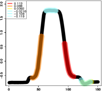
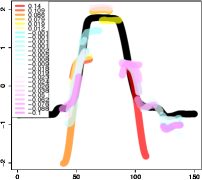
(a) (b)

Figure 1: Examples of the visualization for a time series of Gun-Point data. Both (a) and (b) images are same time series (black line) but the scale is different. (a) Each colored line is a subsequence that maximizes the similarity with some shapelet in a classifier. Subsequences with positive values (red to yellow) contribute the positive class and subsequences with negative values (blue) contribute the negative class. (b)The colored lines show important patterns of output classifier. Positive values on the colored lines (red to yellow) indicate the contribution rate for the positive class, and negative values (blue to purple) indicate the contribution rate for the negative class.

7.2 Results for Multiple-Instance Data

We selected the baselines of MIL algorithms as mi-SVM and MI-SVM (Andrews et al., 2003). Both algorithms are now classical, but still perform favorably compared with state-of-the-art methods for standard multiple-instance data (see, e.g., Doran, 2015). Moreover, the generalization bound of these algorithms are shown in (Sabato and Tishby, 2012) because the algorithms obtain a (single) shapelet-based classifier. Hence, the following comparative experiments simulate a single shapelet with theoretical generalization ability versus infinitely many shapelets with theoretical generalization ability. We combined a linear, polynomial, and Gaussian kernel with mi-SVM and MI-SVM, respectively. Parameter $C$ was chosen from $\{1,10,100,1000,10000\}$, degree $p$ of the polynomial kernel is chosen from $\{2,3,4,5\}$ and parameter $\sigma$ of the Gaussian kernel was chosen from $\{0.001,0.005,0.01,0.05,0.1,0.5,1.0\}$. For our method, we chose $\nu$ from $\{0.5,0.3,0.2,0.15,0.1\}$, and we only used the Gaussian kernel. We chose $\sigma$ from $\{0.005,0.01,0.05,0.1,0.5,1.0\}$. Although we demonstrated both non-sparse and sparse weak learning, interestingly, sparse version beat non-sparse version for all datasets. Thus, we will only show the result on the sparse version because of space limitations. For all these algorithms, we estimated optimal parameter set via 5-fold cross-validation. We used well-known multiple-instance data as shown on the left-hand side of Table 2. The accuracies resulted from 10 runs of 10-fold cross-validation.

The results are shown in the right-hand side of Table 2. Because of space limitations, for baselines we only show the results of the kernel that achieved the best accuracy. Although the accuracy of our method for fox data was slightly worse, our method significantly outperformed baselines for the other 4 datasets.

A Supplementary materials

A.1 Proof of Theorem 1

Definition 1

[The set $\Theta$ of mappings from a bag to an instance]
Given a sample $S=(B_{1},\dots,B_{m})$. For any ${\bf u}\in U$, let $\theta_{{\bf u},\Phi}:\{B_{1},\ldots,B_{m}\}\to\mathcal{X}$ be a mapping defined by

$$\theta_{{\bf u},\Phi}(B_{i}):=\arg\max_{x\in B_{i}}\left\langle{\bf u},\Phi\left(x\right)\right\rangle,$$

and we define the set of all $\theta_{{\bf u},\Phi}$ for $S$ as $\Theta_{S,\Phi}=\{\theta_{{\bf u},\Phi}\mid{\bf u}\in U\}$. For the sake of brevity, $\theta_{{\bf u},\Phi}$ and $\Theta_{S,\Phi}$ will be abbreviated as $\theta_{{\bf u}}$ and $\Theta$, respectively.

Proof  We can rewrite the optimization problem (6) by using $\theta\in\Theta$ as follows:

$$\max_{\theta\in\Theta}\max_{{\bf u}\in\mathbb{H}:\theta_{\bf u}=\theta}\quad \sum_{i=1}^{m}y_{i}d_{i}\left\langle{\bf u},\Phi\left(\theta(B_{i})\right)\right\rangle$$ (10)

sub.to $$\|{\bf u}\|_{\mathbb{H}}^{2}\leq 1.$$

Thus, if we fix $\theta\in\Theta$, we have a sub-problem. Since the constraint $\theta=\theta_{\bf u}$ can be written as the number $|P_{S}|$ of linear constraints, each sub-problem is equivalent to a convex optimization. Indeed, each sub-problem can be written as the equivalent unconstrained minimization (by neglecting constants in the objective)

$$\min_{{\bf u}\in\mathbb{H}}~{} \beta\|{\bf u}\|^{2}_{\mathbb{H}}-\sum_{i=1}^{m}\sum_{x\in B_{i}}\left(\eta_{i,x}\left\langle{\bf u},\Phi\left(\theta(B_{i})\right)\right\rangle-\left\langle{\bf u},\Phi(x)\right\rangle\right)$$

$$-\sum_{i=1}^{m}y_{i}d_{i}\left\langle{\bf u},\Phi\left(\theta(B_{i})\right)\right\rangle$$

sub.to $$\langle{\bf u},\Phi(x)\rangle\leq\langle{\bf u},\Phi(\theta(B_{i}))\rangle\;(i\in[m],x\in B_{i}),$$

where $\beta$ and $\eta_{i,x}$ $(i\in[m],x\in B_{i})$ are the corresponding positive constants. Now for each sub-problem, we can apply the standard Representer Theorem argument (see, e.g., Mohri et al. (2012)). Let $\mathbb{H}_{1}$ be the subspace $\{{\bf u}\in\mathbb{H}\mid{\bf u}=\sum_{z\in P_{S}}\alpha_{z}\Phi(z),\alpha_{z}\in\mathbb{R}\}$. We denote ${\bf u}_{1}$ as the orthogonal projection of ${\bf u}$ onto $\mathbb{H}_{1}$ and any ${\bf u}\in\mathbb{H}$ has the decomposition ${\bf u}={\bf u}_{1}+{\bf u}^{\perp}$. Since ${\bf u}^{\perp}$ is orthogonal w.r.t. $\mathbb{H}_{1}$, $\|{\bf u}\|_{\mathbb{H}}^{2}=\|{\bf u}_{1}\|_{\mathbb{H}}^{2}+\|{\bf u}^{\perp}\|_{\mathbb{H}}^{2}\geq\|{\bf u}_{1}\|_{\mathbb{H}}^{2}$. On the other hand, $\left\langle{\bf u},\Phi\left(z\right)\right\rangle=\left\langle{\bf u}_{1},\Phi\left(z\right)\right\rangle$. Therefore, the optimal solution of each sub-problem has to be contained in $\mathbb{H}_{1}$. This implies that the optimal solution, which is the maximum over all solutions of sub-problems, is contained in $\mathbb{H}_{1}$ as well.  

A.2 Proof of Theorem 2

We use $\theta$ and $\Theta$ of Definition 1.

Definition 2

[The Rademacher and the Gaussian complexity Bartlett and Mendelson (2003)]
Given a sample $S=(x_{1},\dots,x_{m})\in\mathcal{X}^{m}$, the empirical Rademacher complexity $\mathfrak{R}(H)$ of a class $H\subset\{h:\mathcal{X}\to\mathbb{R}\}$ w.r.t. $S$ is defined as $\mathfrak{R}_{S}(H)=\frac{1}{m}\mathop{\rm E}\limits_{\boldsymbol{\sigma}}\left[\sup_{h\in H}\sum_{i=1}^{m}\sigma_{i}h(x_{i})\right]$, where $\boldsymbol{\sigma}\in\{-1,1\}^{m}$ and each $\sigma_{i}$ is an independent uniform random variable in $\{-1,1\}$. The empirical Gaussian complexity $\mathfrak{G}_{S}(H)$ of $H$ w.r.t. $S$ is defined similarly but each $\sigma_{i}$ is drawn independently from the standard normal distribution.

The following bounds are well-known.

Lemma 1

[Lemma 4 of Bartlett and Mendelson (2003)] $\mathfrak{R}_{S}(H)=O(\mathfrak{G}_{S}(H))$.

Lemma 2

[Corollary 6.1 of Mohri et al. (2012)] For fixed $\rho$, $\delta>0$, the following bound holds with probability at least $1-\delta$: for all $f\in\mathrm{conv}(H)$,

$$\mathcal{E}_{D}(f)\leq\mathcal{E}_{\rho}(f)+\frac{2}{\rho}\mathfrak{R}_{S}(H)+3\sqrt{\frac{\log\frac{1}{\delta}}{2m}}.$$

To derive generalization bound based on the Rademacher or the Gaussian complexity is quite standard in the statistical learning theory literature and applicable to our classes of interest as well. However, a standard analysis provides us sub-optimal bounds.

Lemma 3

Suppose that for any $z\in\mathcal{X}$, $\|\Phi(z)\|_{\mathbb{H}}\leq R$. Then, the empirical Gaussian complexity of $H_{U}$ with respect to $S$ for $U\subseteq\{{\bf u}\mid\|{\bf u}\|_{\mathbb{H}}\leq 1\}$ is bounded as follows:

$$\mathfrak{G}_{S}(H)\leq\frac{R\sqrt{(\sqrt{2}-1)+2(\ln|\Theta|)}}{\sqrt{m}}.$$

Proof  Since $U$ can be partitioned into $\bigcup_{\theta\in\Theta}\{{\bf u}\in U\mid\theta_{\bf u}=\theta\}$,

$$\mathfrak{G}_{S}(H_{U}) =\frac{1}{m}\mathop{\rm E}\limits_{\boldsymbol{\sigma}}\left[\sup_{\theta\in\Theta}\sup_{{\bf u}\in U:\theta_{{\bf u}}=\theta}\sum_{i=1}^{m}\sigma_{i}\left\langle{\bf u},\Phi\left(\theta(B_{i})\right)\right\rangle\right]$$

$$=\frac{1}{m}\mathop{\rm E}\limits_{\boldsymbol{\sigma}}\left[\sup_{\theta\in\Theta}\sup_{{\bf u}\in U:\theta_{{\bf u}}=\theta}\left\langle{\bf u},\left(\sum_{i=1}^{m}\sigma_{i}\Phi\left(\theta(B_{i})\right)\right)\right\rangle\right]$$

$$\leq\frac{1}{m}\mathop{\rm E}\limits_{\boldsymbol{\sigma}}\left[\sup_{\theta\in\Theta}\sup_{{\bf u}\in U}\left\langle{\bf u},\left(\sum_{i=1}^{m}\sigma_{i}\Phi\left(\theta(B_{i})\right)\right)\right\rangle\right]$$

$$\leq\frac{1}{m}\mathop{\rm E}\limits_{\boldsymbol{\sigma}}\left[\sup_{\theta\in\Theta}\left\|\sum_{i=1}^{m}\sigma_{i}\Phi\left(\theta(B_{i})\right)\right\|_{\mathbb{H}}\right]$$

$$=\frac{1}{m}\mathop{\rm E}\limits_{\boldsymbol{\sigma}}\left[\sup_{\theta\in\Theta}\sqrt{\left\|\sum_{i=1}^{m}\sigma_{i}\Phi\left(\theta(B_{i})\right)\right\|_{\mathbb{H}}^{2}}\right]$$

$$=\frac{1}{m}\mathop{\rm E}\limits_{\boldsymbol{\sigma}}\left[\sqrt{\sup_{\theta\in\Theta}\left\|\sum_{i=1}^{m}\sigma_{i}\Phi\left(\theta(B_{i})\right)\right\|_{\mathbb{H}}^{2}}\right]$$

$$\leq\frac{1}{m}\sqrt{\mathop{\rm E}\limits_{\boldsymbol{\sigma}}\left[\sup_{\theta\in\Theta}\left\|\sum_{i=1}^{m}\sigma_{i}\Phi\left(\theta(B_{i})\right)\right\|_{\mathbb{H}}^{2}\right]}.$$ (11)

The first inequality is derived from the relaxation of ${\bf u}$, the second inequality is due to Cauchy-Schwarz inequality and the fact $\|{\bf u}\|_{\mathbb{H}}\leq 1$, and the last inequality is due to Jensen’s inequality. We denote by $\boldsymbol{\mathrm{K}}^{(\theta)}$ the kernel matrix such that $\boldsymbol{\mathrm{K}}_{ij}^{(\theta)}=\langle\Phi((\theta(B_{i})),\Phi(\theta(B_{j}))\rangle$. Then, we have

$$\mathop{\rm E}\limits_{\boldsymbol{\sigma}}\left[\sup_{\theta\in\Theta}\left\|\sum_{i=1}^{m}\sigma_{i}\Phi\left(\theta(B_{i})\right)\right\|_{\mathbb{H}}^{2}\right]=\mathop{\rm E}\limits_{\boldsymbol{\sigma}}\left[\sup_{\theta\in\Theta}\sum_{i,j=1}^{m}\sigma_{i}\sigma_{j}\boldsymbol{\mathrm{K}}_{ij}^{(\theta)}\right].$$ (12)

We now derive an upper bound of the r.h.s. as follows.

For any $c>0$,

$$\exp\left(c\mathop{\rm E}\limits_{\boldsymbol{\sigma}}\left[\sup_{\theta\in\Theta}\sum_{i,j=1}^{m}\sigma_{i}\sigma_{j}\boldsymbol{\mathrm{K}}_{ij}^{(\theta)}\right]\right)$$

$$\leq\mathop{\rm E}\limits_{\boldsymbol{\sigma}}\left[\exp\left(c\sup_{\theta\in\Theta}\sum_{i,j=1}^{m}\sigma_{i}\sigma_{j}\boldsymbol{\mathrm{K}}_{ij}^{(\theta)}\right)\right]$$

$$= \mathop{\rm E}\limits_{\boldsymbol{\sigma}}\left[\sup_{\theta\in\Theta}\exp\left(c\sum_{i,j=1}^{m}\sigma_{i}\sigma_{j}\boldsymbol{\mathrm{K}}_{ij}^{(\theta)}\right)\right]$$

$$\leq\sum_{\theta\in\Theta}\mathop{\rm E}\limits_{\boldsymbol{\sigma}}\left[\exp\left(c\sum_{i,j=1}^{m}\sigma_{i}\sigma_{j}\boldsymbol{\mathrm{K}}_{ij}^{(\theta)}\right)\right]$$

The first inequality is due to Jensen’s inequality, and the second inequality is due to the fact that the supremum is bounded by the sum. By using the symmetry property of $\boldsymbol{\mathrm{K}}^{(\theta)}$, we have $\sum_{i,j=1}^{m}\sigma_{i}\sigma_{j}\boldsymbol{\mathrm{K}}_{ij}^{(\theta)}=\boldsymbol{\sigma}^{\top}\boldsymbol{\mathrm{K}}^{(\theta)}\boldsymbol{\sigma}$, which is rewritten as

$$\boldsymbol{\sigma}^{\top}\boldsymbol{\mathrm{K}}^{(\theta)}\boldsymbol{\sigma}=(\boldsymbol{\mathrm{V}}^{\top}\boldsymbol{\sigma})^{\top}\left(\begin{array}[]{ccc}\lambda_{1}^{(\theta)}&\hfill\hfil&0\\ \hfill\hfil&\ddots&\hfill\hfil\\ 0&\hfill\hfil&\lambda_{m}^{(\theta)}\\ \end{array}\right)\boldsymbol{\mathrm{V}}^{\top}\boldsymbol{\sigma},$$

where $\lambda_{1}^{(\theta)}\geq\dots\geq\lambda_{m}^{(\theta)}\geq 0$ are the eigenvalues of $\boldsymbol{\mathrm{K}}^{(\theta)}$ and $\boldsymbol{\mathrm{V}}=({\bf v}_{1},\ldots,{\bf v}_{m})$ is the orthonormal matrix such that ${\bf v}_{i}$ is the eigenvector that corresponds to the eigenvalue $\lambda_{i}$. By the reproductive property of Gaussian distribution, $\boldsymbol{\mathrm{V}}^{\top}\boldsymbol{\sigma}$ obeys the same Gaussian distribution as well. So,

$$\sum_{\theta\in\Theta}\mathop{\rm E}\limits_{\boldsymbol{\sigma}}\left[\exp\left(c\sum_{i,j=1}^{m}\sigma_{i}\sigma_{j}\boldsymbol{\mathrm{K}}_{ij}^{(\theta)}\right)\right]$$

$$= \sum_{\theta\in\Theta}\mathop{\rm E}\limits_{\boldsymbol{\sigma}}\left[\exp\left(c\boldsymbol{\sigma}^{\top}\boldsymbol{\mathrm{K}}^{(\theta)}\boldsymbol{\sigma}\right)\right]$$

$$= \sum_{\theta\in\Theta}\mathop{\rm E}\limits_{\boldsymbol{\sigma}}\left[\exp\left(c\sum_{k=1}^{m}\lambda_{k}^{(\theta)}({\bf v}_{k}^{\top}\boldsymbol{\sigma})^{2}\right)\right]$$

$$= \sum_{\theta\in\Theta}\Pi_{k=1}^{m}\mathop{\rm E}\limits_{\sigma_{k}}\left[\exp\left(c\lambda_{k}^{(\theta)}\sigma_{k}^{2}\right)\right]~{}~{}(\text{replace}~{}\boldsymbol{\sigma}={\bf v}_{k}^{\top}\boldsymbol{\sigma})$$

$$= \sum_{\theta\in\Theta}\Pi_{k=1}^{m}\left(\int_{-\infty}^{\infty}\exp\left(c\lambda_{k}^{(\theta)}\sigma^{2}\right)\frac{\exp(-\sigma^{2})}{\sqrt{2\pi}}d\sigma\right)$$

$$= \sum_{\theta\in\Theta}\Pi_{k=1}^{m}\left(\int_{-\infty}^{\infty}\frac{\exp(-(1-c\lambda_{k}^{(\theta)})\sigma^{2})}{\sqrt{2\pi}}d\sigma\right).$$

Now we replace $\sigma$ by $\sigma^{\prime}=\sqrt{1-c\lambda_{k}^{(\theta)}}\sigma$. Since $d\sigma^{\prime}=\sqrt{1-c\lambda_{k}^{(\theta)}}d\sigma$, we have:

$$\int_{-\infty}^{\infty}\frac{\exp(-(1-c\lambda_{k}^{(\theta)})\sigma^{2})}{\sqrt{2}\pi}d\sigma=\frac{1}{\sqrt{2\pi}}\int_{-\infty}^{\infty}\frac{\exp(-\sigma^{\prime 2})}{\sqrt{1-c\lambda_{k}^{(\theta)}}}d\sigma^{\prime}$$

$$= \frac{1}{\sqrt{1-c\lambda_{k}^{(\theta)}}}.$$

Now, applying the inequality that $\frac{1}{\sqrt{1-x}}\leq 1+2(\sqrt{2}-1)x$ for $0\leq x\leq\frac{1}{2}$, the bound becomes

$$\exp\left(c\mathop{\rm E}\limits_{\boldsymbol{\sigma}}\left[\sup_{\theta\in\Theta}\sum_{i,j=1}^{m}\sigma_{i}\sigma_{j}\boldsymbol{\mathrm{K}}_{ij}^{(\theta)}\right]\right)$$

$$\leq \sum_{\theta\in\Theta}\Pi_{k=1}^{m}\left(1+2(\sqrt{2}-1)c\lambda_{k}^{(\theta)}+2\lambda_{1}\right).$$ (13)

Further, taking logarithm, dividing the both sides by $c$, letting $c=\frac{1}{2\max_{k}\lambda_{k}^{(\theta)}}=1/(2\lambda_{1}^{(\theta)})$, fix $\theta=\theta^{*}$ such that $\theta^{*}$ maximizes (A.2), and applying $\ln(1+x)\leq x$, we get:

$$\mathop{\rm E}\limits_{\boldsymbol{\sigma}}\left[\sup_{\theta\in\Theta}\sum_{i,j=1}^{m}\sigma_{i}\sigma_{j}\boldsymbol{\mathrm{K}}_{ij}^{(\theta^{*})}\right]$$

$$\leq(\sqrt{2}-1)\sum_{k=1}^{m}\lambda_{k}^{(\theta^{*})}+2\lambda_{1}^{(\theta^{*})}\ln|\Theta|$$

$$=(\sqrt{2}-1)\mathrm{tr}(\boldsymbol{\mathrm{K}}^{(\theta^{*})})+2\lambda_{1}^{(\theta^{*})}\ln|\Theta|$$

$$\leq(\sqrt{2}-1)mR^{2}+2mR^{2}\ln|\Theta|,$$ (14)

where the last inequality holds since $\lambda_{1}^{(\theta^{*})}=\|\boldsymbol{\mathrm{K}}^{(\theta^{*})}\|_{2}\leq m\|\boldsymbol{\mathrm{K}}^{(\theta)}\|_{\max}\leq R^{2}$. By equation (A.2) and (A.2), we have:

$$\mathfrak{G}_{S}(H) \leq\frac{1}{m}\sqrt{\mathop{\rm E}\limits_{\boldsymbol{\sigma}}\left[\sup_{\theta\in\Theta}\sum_{i,j=1}^{m}\sigma_{i}\sigma_{j}\boldsymbol{\mathrm{K}}_{ij}^{(\theta)}\right]}$$

$$\leq\frac{R\sqrt{(\sqrt{2}-1)+2\ln|\Theta|}}{\sqrt{m}}.$$

 

Thus, it suffices to bound the size $|\Theta|$. The basic idea to get our bound is the following geometric analysis. Fix any $i\in[m]$ and consider points $\{\Phi(x)\mid x\in B_{i}\}$. Then, we define equivalence classes of ${\bf u}$ such that $\theta_{\bf u}(i)$ is in the same class, which define a Voronoi diagram for the points $\{\Phi(x)\mid x\in B_{i}\}$. Note here that the similarity is measured by the inner product, not a distance. More precisely, let $V(B_{i})=\{V(x)\mid x\in B\}$ be the Voronoi diagram, each of the region is defined as $V(x)=\{{\bf u}\in\mathbb{H}\mid\theta_{{\bf u}}(B_{i})=x\}$ Let us consider the set of intersections $\bigcap_{i\in[m]}V_{i}{(x_{i})}$ for all combinations of $(x_{1},\ldots,x_{m})\in B_{1}\times\cdots\times B_{m}$. The key observation is that each non-empty intersection corresponds to a mapping $\theta_{{\bf u}}\in\Theta$. Thus, we obtain $|\Theta|=(\text{the number of intersections $\bigcap_{i\in[m]}V_{i}(x_{i})$})$. In other words, the size of $\Theta$ is exactly the number of rooms defined by the intersections of $m$ Voronoi diagrams $V_{1},\dots,V_{m}$. From now on, we will derive upper bound based on this observation.

Lemma 4

$$|\Theta|=O(|P_{S}|^{2d_{\Phi,S}^{*}}).$$

Proof  We will reduce the problem of counting intersections of the Voronoi diagrams to that of counting possible labelings by hyperplanes for some set. Note that for each neighboring Voronoi regions, the border is a part of hyperplane since the closeness is defined in terms of the inner product. Therefore, by simply extending each border to a hyperplane, we obtain intersections of halfspaces defined by the extended hyperplanes. Note that, the size of these intersections gives an upper bound of intersections of the Voronoi diagrams. More precisely, we draw hyperplanes for each pair of points in $\Phi(P_{S})$ so that each point on the hyperplane has the same inner product between two points. Note that for each pair $\Phi(z),\Phi(z^{\prime})\in P_{S}$, the normal vector of the hyperplane is given as $\Phi(z)-\Phi(z^{\prime})$ (by fixing the sign arbitrary). Thus, the set of hyperplanes obtained by this procedure is exactly $\Phi_{\mathrm{diff}}(P_{S})$. The size of $\Phi_{\mathrm{diff}}(P_{S})$ is ${|P_{S}|}\choose 2$, which is at most $|P_{S}|^{2}$. Now, we consider a “dual” space by viewing each hyperplane as a point and each point in $U$ as a hyperplane. Note that points ${\bf u}$ (hyperplanes in the dual) in an intersection give the same labeling on the points in the dual domain. Therefore, the number of intersections in the original domain is the same as the number of the possible labelings on $\Phi_{\mathrm{diff}}(P_{S})$ by hyperplanes in $U$. By the classical Sauer’s Lemma and the VC dimension of hyperplanes (see, e.g., Theorem 5.5 in Schölkopf and Smola (2002)), the size is at most $O((|P_{S}|^{2})^{d_{\Phi,S}^{*}})$.  

Theorem 4

1. For any $\Phi$, $|\Theta|=O(|P_{S}|^{8(R/\mu^{*})^{2}})$.

2. if $\mathcal{X}\subseteq\mathbb{R}^{\ell}$ and $\Phi$ is the identity mapping over $P_{S}$, then $|\Theta|=O(|P_{S}|^{\min\{8(R/\mu^{*})^{2},2\ell\}}\})$.

3. if $\mathcal{X}\subseteq\mathbb{R}^{\ell}$ and $\Phi$ satisfies that $\left\langle\Phi(z),\Phi(x)\right\rangle$ is monotone decreasing with respect to $\|z-x\|_{2}$ (e.g., the mapping defined by the Gaussian kernel) and $U=\{\Phi(z)\mid z\in\mathcal{X}\subseteq\mathbb{R}^{\ell},\|\Phi(z)\|_{\mathbb{H}}\leq 1\}$, then $|\Theta|=O(|P_{S}|^{\min\{8(R/\mu^{*})^{2},2\ell\}}\})$.

Proof  (i) We follow the argument in Lemma 4. For the set of classifiers $F=\{f:\Phi_{\mathrm{diff}}(P_{S})\to\{-1,1\}\mid f=\mathrm{sign}(\langle{\bf u},{\bf v}\rangle),\|{\bf u}\|_{\mathbb{H}}\leq 1,\min_{{\bf v}\in\Phi_{\mathrm{diff}}(P_{S})}|\langle{\bf u},{\bf v}\rangle|=\mu\}$, its VC dimension is known to be at most $R^{2}/\mu^{2}$ for $\Phi_{\mathrm{diff}}(P_{S})\subseteq\{{\bf v}\mid\|{\bf v}\|_{\mathbb{H}}\leq 2R\}$ (see, e.g., Schölkopf and Smola (2002)). By the definition of $\mu^{*}$, for each intersections given by hyperplanes, there always exists a point ${\bf u}$ whose inner product between each hyperplane is at least $\mu^{*}$. Therefore, the size of the intersections is bounded by the number of possible labelings in the dual space by $U^{\prime\prime}=\{{\bf u}\in\mathbb{H}\mid\|{\bf u}\|_{\mathbb{H}}\leq 1,\min_{{\bf v}\in\Phi_{\mathrm{diff}}(P_{S})}|\langle{\bf u},{\bf v}\rangle|=\mu^{*}\}$. Thus we obtain that $d_{\Phi,S}^{*}$ is at most $8(R/\mu^{*})^{2}$ and by Lemma 4, we complete the proof of case (i).

(ii) In this case, the Hilbert space $\mathbb{H}$ is contained in $\mathbb{R}^{\ell}$. Then, by the fact that VC dimension $d_{\Phi,S}^{*}$ is at most $\ell$ and Lemma 4, the statement holds.

(iii) If $\left\langle\Phi(z),\Phi(x)\right\rangle$ is monotone decreasing for $\|z-x\|$, then the following holds:

$$\arg\max_{x\in\mathcal{X}}\left\langle\Phi(z),\Phi(x)\right\rangle=\arg\min_{x\in\mathcal{X}}\|z-x\|_{2}.$$

Therefore, $\max_{{\bf u}:\|{\bf u}\|_{\mathbb{H}}=1}\langle{\bf u},\Phi(x)\rangle=\|\Phi(x)\|_{\mathbb{H}}$, where ${\bf u}=\frac{\Phi(x)}{\|\Phi(x)\|_{\mathbb{H}}}$. It indicates that the number of Voronoi cells made by $V(x)=\{z\in\mathbb{R}^{\ell}\mid z=\arg\max_{x\in B}(z\cdot x)\}$ corresponds to the $\hat{V}(x)=\{\Phi(z)\in\mathbb{H}\mid z=\arg\max_{x\in B}\langle\Phi(z),\Phi(x)\rangle\}$. Then, by following the same argument for the linear kernel case, we get the same statement.  
Now we are ready to prove Theorem 2.

Proof [Proof of Theorem 2] By using Lemma 1, and 2, we obtain the generalization bound in terms of the Gaussian complexity of $H$. Then, by applying Lemma 3 and Theorem 4, we complete the proof.  

A.3 Heuristics for Improving Efficiency

For large multiple-instance data such as time-series data that may contain a lot of subsequences, we need to reduce the computational cost of weak learning in Algorithm 2. Therefore, we introduce two heuristic options for improving efficiency. First, in Algorithm 2, we fix an initial $\boldsymbol{\alpha}_{0}$ as following: More precisely, we initially solve

$$\boldsymbol{\alpha}_{0}=\arg\max_{\boldsymbol{\alpha}} \sum_{i=1}^{m}d_{i}y_{i}\max_{x\in B_{i}}\sum_{z\in P_{S}}\alpha_{z}K\left(z,x\right),$$

sub.to $$~{}~{}\boldsymbol{\alpha}~{}\text{is a one-hot vector.}$$

That is, we choose the most discriminative shapelet from $P_{S}$ as the initial point of ${\bf u}$ for given ${\bf d}$. We expect that it will speed up the convergence of the loop of line 3, and the obtained classifier is better than the methods that choose effective shapelets from subsequences. For Gun-Point data described in Table 1, this method obtains the solution approximately seven times faster than when random vectors are used as the initial $\boldsymbol{\alpha}_{0}$.

Second, we reduce the high computational cost induced by calculating $\sum_{z\in P_{S}}d_{k}\alpha_{z}K\left(z,x\right)$ in our problem. For example, when we consider subsequences as instances for time series classification, we have a large computational cost because of the number of subsequences of training data (e.g., approximately $10^{6}$ when sample size is $1000$ and length of each time series is $1000$, which results in a similarity matrix of size $10^{12}$). However, in most cases, many subsequences in time series data are similar to each other. Therefore, we only use representative instances $\hat{P}_{S}$ instead of the set of all instances $P_{S}$. In these experiments, we extract $\hat{P}_{S}$ via $k$-means clustering of $P_{S}$. Although this approach may decrease the classification accuracy, it drastically decreases the computational cost for a large dataset. For the Gun-Point dataset, this approach with $k=10$ still achieves high classification accuracy and it is over $2000$ times faster on average than when all of subsequences are used. In our experiments including the MIL task, we use $100$-means clustering to obtain the representative instances. Surprisingly, as demonstrated in the experiments, these heuristics work well not only for time-series data but also for multiple-instance data in practice.

References

- Andrews and Hofmann (2004) Stuart Andrews and Thomas Hofmann. Multiple instance learning via disjunctive programming boosting. In S. Thrun, L. K. Saul, and B. Schölkopf, editors, Advances in Neural Information Processing Systems 16, pages 65–72. MIT Press, 2004.
- Andrews et al. (2003) Stuart Andrews, Ioannis Tsochantaridis, and Thomas Hofmann. Support vector machines for multiple-instance learning. In S. Becker, S. Thrun, and K. Obermayer, editors, Advances in Neural Information Processing Systems 15, pages 577–584. MIT Press, 2003.
- Auer and Ortner (2004) Peter Auer and Ronald Ortner. A boosting approach to multiple instance learning. In Jean-Fran¥ccois Boulicaut, Floriana Esposito, Fosca Giannotti, and Dino Pedreschi, editors, Machine Learning: ECML 2004, pages 63–74, Berlin, Heidelberg, 2004. Springer Berlin Heidelberg.
- Bagnall et al. (2017) Anthony Bagnall, Jason Lines, Aaron Bostrom, James Large, and Eamonn Keogh. The great time series classification bake off: a review and experimental evaluation of recent algorithmic advances. Data Mining and Knowledge Discovery, 31(3):606–660, May 2017. ISSN 1573-756X.
- Bartlett and Mendelson (2003) Peter L. Bartlett and Shahar Mendelson. Rademacher and gaussian complexities: Risk bounds and structural results. Journal of Machine Learning Research, 3:463–482, 2003.
- Carbonneau et al. (2018) Marc-André Carbonneau, Veronika Cheplygina, Eric Granger, and Ghyslain Gagnon. Multiple instance learning: A survey of problem characteristics and applications. Pattern Recognition, 77:329 – 353, 2018. ISSN 0031-3203.
- Chen et al. (2015) Yanping Chen, Eamonn Keogh, Bing Hu, Nurjahan Begum, Anthony Bagnall, Abdullah Mueen, and Gustavo Batista. The ucr time series classification archive, July 2015. www.cs.ucr.edu/~eamonn/time_series_data/.
- Chen et al. (2006) Yixin Chen, Jinbo Bi, and J. Z. Wang. Miles: Multiple-instance learning via embedded instance selection. IEEE Transactions on Pattern Analysis and Machine Intelligence, 28(12):1931–1947, Dec 2006. ISSN 0162-8828.
- Demiriz et al. (2002) A Demiriz, K P Bennett, and J Shawe-Taylor. Linear Programming Boosting via Column Generation. Machine Learning, 46(1-3):225–254, 2002.
- Dietterich et al. (1997) Thomas G. Dietterich, Richard H. Lathrop, and Tomás Lozano-Pérez. Solving the multiple instance problem with axis-parallel rectangles. Artificial Intelligence, 89(1-2):31–71, January 1997. ISSN 0004-3702.
- Doran (2015) Gary Doran. Multiple Instance Learning from Distributions. PhD thesis, Case WesternReserve University, 2015.
- Doran and Ray (2014) Gary Doran and Soumya Ray. A theoretical and empirical analysis of support vector machine methods for multiple-instance classification. Machine Learning, 97(1-2):79–102, October 2014. ISSN 0885-6125.
- Gärtner et al. (2002) Thomas Gärtner, Peter A. Flach, Adam Kowalczyk, and Alex J. Smola. Multi-instance kernels. In Proceedings 19th International Conference. on Machine Learning, pages 179–186. Morgan Kaufmann, 2002.
- Grabocka et al. (2014) Josif Grabocka, Nicolas Schilling, Martin Wistuba, and Lars Schmidt-Thieme. Learning time-series shapelets. In Proceedings of the 20th ACM SIGKDD International Conference on Knowledge Discovery and Data Mining, KDD ’14, pages 392–401, 2014.
- Grabocka et al. (2015) Josif Grabocka, Martin Wistuba, and Lars Schmidt-Thieme. Scalable discovery of time-series shapelets. CoRR, abs/1503.03238, 2015.
- Hills et al. (2014) Jon Hills, Jason Lines, Edgaras Baranauskas, James Mapp, and Anthony Bagnall. Classification of time series by shapelet transformation. Data Mining and Knowledge Discovery, 28(4):851–881, July 2014. ISSN 1384-5810.
- Hou et al. (2016) Lu Hou, James T. Kwok, and Jacek M. Zurada. Efficient learning of timeseries shapelets. In Proceedings of the Thirtieth AAAI Conference on Artificial Intelligence,, pages 1209–1215, 2016.
- Keogh and Rakthanmanon (2013) Eamonn J. Keogh and Thanawin Rakthanmanon. Fast shapelets: A scalable algorithm for discovering time series shapelets. In Proceedings of the 13th SIAM International Conference on Data Mining, pages 668–676, 2013.
- Mohri et al. (2012) Mehryar Mohri, Afshin Rostamizadeh, and Ameet Talwalkar. Foundations of Machine Learning. The MIT Press, 2012.
- Platt et al. (2000) John C. Platt, Nello Cristianini, and John Shawe-Taylor. Large margin dags for multiclass classification. In S. A. Solla, T. K. Leen, and K. M¥”uller, editors, Advances in Neural Information Processing Systems 12, pages 547–553. MIT Press, 2000.
- Renard et al. (2015) Xavier Renard, Maria Rifqi, Walid Erray, and Marcin Detyniecki. Random-shapelet: an algorithm for fast shapelet discovery. In 2015 IEEE International Conference on Data Science and Advanced Analytics (IEEE DSAA’2015), pages 1–10. IEEE, 2015.
- Sabato and Tishby (2012) Sivan Sabato and Naftali Tishby. Multi-instance learning with any hypothesis class. Journal of Machine Learning Research, 13(1):2999–3039, October 2012. ISSN 1532-4435.
- Schölkopf and Smola (2002) B. Schölkopf and AJ. Smola. Learning with Kernels: Support Vector Machines, Regularization, Optimization, and Beyond. Adaptive Computation and Machine Learning. MIT Press, Cambridge, MA, USA, December 2002.
- Shapiro (2009) Alexander Shapiro. Semi-infinite programming, duality, discretization and optimality conditions. Optimization, 58(2):133–161, 2009.
- Suehiro et al. (2017) Daiki Suehiro, Kohei Hatano, Eiji Takimoto, Shuji Yamamoto, Kenichi Bannai, and Akiko Takeda. Boosting the kernelized shapelets: Theory and algorithms for local features. CoRR, abs/1709.01300, 2017.
- Tao and Souad (1988) Pham Dinh Tao and El Bernoussi Souad. Duality in D.C. (Difference of Convex functions) Optimization. Subgradient Methods, pages 277–293. Birkhäuser Basel, Basel, 1988.
- Ye and Keogh (2009) Lexiang Ye and Eamonn Keogh. Time series shapelets: A new primitive for data mining. In Proceedings of the 15th ACM SIGKDD International Conference on Knowledge Discovery and Data Mining, KDD ’09, pages 947–956. ACM, 2009.
- Yu and Joachims (2009) Chun-Nam John Yu and Thorsten Joachims. Learning structural svms with latent variables. In Proceedings of the 26th Annual International Conference on Machine Learning, ICML ’09, pages 1169–1176, New York, NY, USA, 2009. ACM. ISBN 978-1-60558-516-1.
- Zhang et al. (2006) Cha Zhang, John C. Platt, and Paul A. Viola. Multiple instance boosting for object detection. In Y. Weiss, B. Schölkopf, and J. C. Platt, editors, Advances in Neural Information Processing Systems 18, pages 1417–1424. MIT Press, 2006.
- Zhang et al. (2013) Dan Zhang, Jingrui He, Luo Si, and Richard Lawrence. Mileage: Multiple instance learning with global embedding. In Sanjoy Dasgupta and David McAllester, editors, Proceedings of the 30th International Conference on Machine Learning, volume 28 of Proceedings of Machine Learning Research, pages 82–90, Atlanta, Georgia, USA, 17–19 Jun 2013. PMLR.