Unzipping DNA by a periodic force: Hysteresis loops, Dynamical order parameter, Correlations and Equilibrium curves

Abstract

The unzipping of a double stranded DNA whose ends are subjected to a time dependent periodic force with frequency $\omega$ and amplitude $G$ is studied using Monte Carlo simulations. We obtain the dynamical order parameter, $Q$, defined as the time average extension between the end monomers of two strands of the DNA over a period, and its probability distributions $P(Q)$ at various force amplitudes and frequencies. We also study the time autocorrelations of extension and the dynamical order parameter for various chain lengths. The equilibrium force-distance isotherms were also obtained at various frequencies by using non-equilibrium work measurements.

I Introduction

The unzipping of a double stranded DNA (dsDNA) is a crucial step in biological processes like DNA replication and RNA transcription. This is achieved in vivo by enzymes like helicases and polymerases Watson2003 . In the last two decades there have been several in vitro experimental studies (see Smith1996 ; Wang1997 ; Roulet1997 ; Bockelmann2002 ; Danilowicz2004 ; Ritort2006 and references therein) on unzipping transitions due to the development of single molecule manipulation techniques such as atomic force microscopy, optical and magnetic tweezers, etc. These studies have been supplemented by theoretical modeling Bhattacharjee2000 ; Lubensky2000 ; Sebastian2000 ; Marenduzzo2001 ; Marenduzzo2002 ; Kapri2004 ; Kapri2006 ; Kapri2007 ; Kapri2008 ; Kapri2009 ; Kumar2010 ; Kalyan2015 which have provided useful insights into the problem including the unzipping phase diagram Marenduzzo2002 ; Kapri2004 . It was found that the unzipping of a dsDNA is a first order phase transition implying that the DNA remains in a zipped phase unless the force that pulls apart its strands exceeds a critical value Bhattacharjee2000 ; Lubensky2000 . Above this critical force, the DNA is in the unzipped phase in which the strands are far apart. The critical force depends on the temperature of the surrounding and decreases to zero when the temperature becomes equal to the melting temperature of the DNA. At this temperature the thermal denaturation of the DNA takes place in which the strands of the DNA remains apart from each other and acquire conformations that increases the entropy of the system.

In recent years, the unzipping studies have shifted toward the periodic forcing of DNA as it is more closer to the phenomenon that occurs in a living cell. The unzipping of DNA inside the cell is a nonequilibrium process initiated by motor proteins called helicases. These motor proteins require a constant supply of energy, obtained from ATP hydrolysis, for their functioning and apply force on the DNA in a cyclic manner Watson2003 (e.g., PcrA helicase Velankar1999 ). This periodic force can cause unbinding and rebinding of biomolecules Hatch2007 ; Li2007 ; Friddle2008 ; Tshiprut2009 ; Min2013 that can provide useful information on the kinetics of conformational transformations, the potential energy landscape, and can be used in controlling the folding pathways of a single molecule Li2007 . By applying a periodic force on the ends of the DNA, it was found using Langevin dynamics Mishra2013 ; Sanjay2013 ; Rakesh2013 ; Sanjay2016 ; Pal2018 and Monte Carlo Kapri2012 ; Kapri2014 simulations on the coarse grained models that the dsDNA can be taken from a zipped to an unzipping phase (or vice versa) dynamically either by changing the frequency of the force and keeping the amplitude constant, or by changing the amplitude of the force and keeping the frequency constant. When the strands of the DNA are pulled away by a periodic force $g(t)$, the extension between the end monomers $x(t)$ follows the force with a lag. The average extension $\langle x(g)\rangle$ when plotted against the magnitude of force $g$ shows a hysteresis loop whose area, which represents the amount of energy dissipated in the system, is a dynamical order parameter Chakrabarti1999 . Hysteresis is usually associated with a first-order phase transition due to the coexistence of two phases at a first-order phase boundary. These two phases are separated by an interface whose energy acts as a barrier between them. Near the phase boundary, there is a region of metastability where the system can stay in its previous phase even after crossing the phase boundary. From the dynamics point of view, the relaxation time or the time scale to cross the barrier becomes large near the transition, and therefore, there is a conflict between relaxation and the time scale of change of parameters, which produces hysteresis.

For systems exhibiting dynamic phase transitions, the time average of the order parameter (extension between the end monomers of two strands for the present case) over a time period also serves as another dynamical order parameter (say $Q$)Chakrabarti1999 . Although there have been many studies on periodic forcing of DNA that have focused on the hysteresis loop area and its scaling with the force amplitude and frequency, Sanjay2013 ; Rakesh2013 ; Kapri2014 ; Sanjay2016 ; Pal2018 there is only one Langevin dynamics simulation study to the best of our knowledge that focuses on the behavior of $Q$. Mishra2013 In this paper we discuss the variation of average dynamical order parameter $\langle Q\rangle$ and the probability distributions $P(Q)$ as a function of frequency and force amplitude using Monte Carlo simulations. We find that the time autocorrelation of extension between the end monomers of two strands behaves with length $N$ as $t/N^{z}$ with dynamic exponent $z=1$ and the dynamical order parameter $Q$ varies with length as $p/N^{z_{p}}$, where $p$ represents the number of time periods of the force, with exponent $z_{p}=2$. We also obtain the equilibrium force-distance isotherms for the DNA using the nonequilibrium work measurements on the trajectories traced by the distance between the end monomers of two strands of the DNA due to periodic forcing.

The paper is organized as follows: In Sec. II, we define our model and the quantities of interest. In Sec. III, we first present our results and discuss them. We summarize our results in Sec. IV.

II Model

The model used in this paper has been used previously to study the unzipping of DNA by periodic forcing. Kapri2012 ; Kapri2014 In this model, the two strands of a homopolymer DNA are represented by two directed self-avoiding walks on a ($d=1+1$)-dimensional square lattice. The walks starting from the origin are restricted to go towards the positive direction of the diagonal axis ($z$-direction) without crossing each other, i.e., in every step, the $z$ coordinate is incremented by 1 and the $x$ coordinate changes by $\pm 1$. The projection of a monomer on the $x-$axis gives its $x$ coordinate. The directional nature of walks takes care of self-avoidance and the correct base pairing of DNA, i.e., the monomers that are complementary to each other are allowed to occupy the same lattice site. For each such overlap there is a gain of energy $-\epsilon$ ($\epsilon>0$). One end of the DNA is anchored at the origin and a time-dependent periodic force

$$g(t)=G\left|\sin\left(\omega t\right)\right|$$ (1)

with angular frequency $\omega$ and amplitude $G$ acts along the transverse direction ($x$ direction) at the free end. Throughout the paper, by frequency we mean the angular frequency. The schematic diagram of the model is shown in Fig. 1.

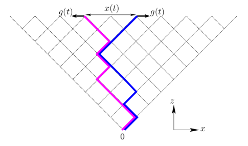
Figure 1: Schematic diagram of the model. The strands of the DNA are shown by thick solid lines. The end monomers of the strands are pulled along $x$ direction with a periodic force $g(t)=G\left|\sin(\omega t)\right|$. The separation between the end monomers, $x(t)$, follows the external force $g(t)$ with a lag.

In the static force limit (i.e., $\omega\to 0$), the model can be solved exactly via generating function and exact transfer matrix techniques, and has been used to obtain the phase diagrams of the DNA unzipping. Marenduzzo2001 ; Marenduzzo2002 ; Kapri2004 For the static force case, the temperature dependent phase boundary is given by

$$g_{c}(T)=-\frac{T}{2}\ln\lambda(z_{2}),$$ (2)

where $\lambda(z)=(1-2z-\sqrt{1-4z})/(2z)$ and $z_{2}=\sqrt{1-e^{-\beta\epsilon}}-1+e^{-\beta\epsilon}$. The zero force melting takes place at a temperature $T_{m}=\epsilon/\ln(4/3)$ (for details see Ref. Kapri2012 ). From Eq. (2), the critical force at temperature $T=1$, which is the temperature used in this study, is obtained as $g_{c}(1)=0.6778\dots$. Although the above model ignores finer details like bending rigidity of the dsDNA, sequence heterogeneity, stacking of base pairs, etc., it was found that the basic features, such as the first order nature of the unzipping transition and the existence of a re-entrant region allowing unzipping by decreasing temperature, are preserved by this two dimensional modelMarenduzzo2001 ; Marenduzzo2002 .

We perform Monte Carlo simulations of the model by using the METROPOLIS algorithm. In our model, the directional nature of the walks prevents the self-crossing of strands. To avoid mutual crossing of strands, we allow strands to undergo Rouse dynamics with local corner-flip or end-flip moves Doi1986 that do not violate mutual avoidance. The elementary move consists of selecting a random monomer from a strand, which itself is chosen at random, and flipping it. If the move results in overlapping of two complementary monomers, thus forming a base-pair between the strands, it is always accepted as a move. The opposite move, i.e., the unbinding of monomers, is chosen with the Boltzmann probability $\xi=\exp(-\varepsilon/k_{B}T)$. If the chosen monomer is unbound and would remain unbound after the move is performed, it is always accepted. The time is measured in units of Monte Carlo Steps (MCSs). One MCS consists of $2N$ flip attempts, i.e., on average, every monomer is given a chance to flip. Throughout the simulation, the detailed balance is always satisfied. From any starting configuration, it is possible to reach any other configuration by using the above moves. Throughout this paper, we have chosen $\varepsilon=1$ and $k_{B}=1$.

At any given frequency $\omega$ and the force amplitude $G$, as the time $t$ is incremented by unity, the external force $g(t)$ changes, according to Eq. (1), from $0$ to a maximum value $G$ and then decreases to $0$. Between each time increment, the system is relaxed by a unit time (1 MCS). Upon further increment in $t$, the above cycle gets repeated again and again. Before taking any measurement, the simulation is run for $2000$ cycles so that the system can reach the stationary state.

In our simulations, we monitor the distance between the end monomers of the two strands, $x(t)$, as a function of time for various force amplitudes $G$ and frequencies $\omega$. Note that a monomer on flipping always goes to the opposite corner of the square lattice in this model. Thus, the distance changes by 2 units (i.e., the length of the diagonal) in each flip. From the time series $x(t)$, we can define a dynamical quantity $Q$ as the time average of $x(t)$ over a complete period

$$Q=\frac{\omega}{\pi}\oint x(t)dt.$$ (3)

Following Chakrabarti and Acharyya, Chakrabarti1999 we call $Q$ as the dynamical order parameter.

From the time series $x(t)$, we can also obtain the extension $x(g)$ as a function of force $g$. Since the force is periodic in nature, one closed loop is obtained per cycle. On averaging over various cycles, we obtain the average extension $\langle x(g)\rangle$. If the force amplitude $G$ is not very small, and the frequency $\omega$ of the periodic force is sufficiently high to avoid equilibration of the DNA, the average extension, $\langle x(g)\rangle$, for the forward and the backward paths is not the same and we see a hysteresis loop. The area of the hysteresis loop, $A_{loop}$, defined by

$$A_{loop}=\oint\langle x(g)\rangle dg,$$ (4)

depends upon the frequency $\omega$ and the amplitude $G$ of the oscillating force and also serves as another dynamical order parameter. Chakrabarti1999

In Ref. Kapri2014 , we have reported the behavior of $A_{loop}$ at high and low frequencies at various force amplitudes $G$ using Monte Carlo simulations. In this paper, we focus mainly on the results related to the dynamical order parameter $Q$.

III Results and Discussions

III.1 Hysteresis loops

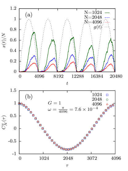
Figure 2: (a) The end-to-end separation $x(t)$ as a function of time $t$ for the DNA of lengths $N=1024$, 2048 and 4096 when it is subjected to a periodic force of amplitude $G=1$ at frequency $\omega=\pi/4096=7.6\times 10^{-4}$. The force variation is shown by thin dotted lines. (b) Data collapse of time autocorrelation function $C_{N}^{x}(\tau)$ of extension $x$, defined in Eq. (5), for various chain lengths $N$ at same frequency and force amplitude as in (a).

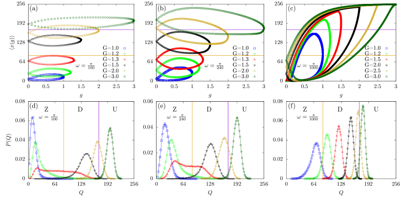
Figure 3: (Top) Average extension $\langle x(g)\rangle$ as a function of force $g$ for various force amplitudes $G$ as indicated with frequencies of pulling (a) $\omega=\pi/100$, (b) $\omega=\pi/240$, and (c) $\omega=\pi/1000$. (Bottom) The normalized probability distribution $P(Q)$ of order parameter $Q$ at frequencies (d) $\omega=\pi/100$, (e) $\omega=\pi/240$, and (f) $\omega=\pi/1000$. The length of the DNA used is $N=128$.

In Fig. 2(a), we have plotted five different cycles of the scaled extension $x(t)/N$ as a function of time $t$ for DNA of various lengths $N=1024$, 2048, and 4096, when it is subjected to a periodic force of amplitude $G=1$ at frequency $\omega=\pi/4096=7.6\times 10^{-4}$. The time required to unzip the DNA is directly proportional to its length. Since the magnitude of the force continues to increase much beyond the critical force $g_{c}$, the unzipped section of the DNA keeps on stretching. For a given frequency and force amplitude, only a finite length of the chain could be unzipped, which is directly proportional to the extension $x(t)$ due to the geometry of the problem. To plot extensions for various chain lengths on the same scale, we divide it by the chain length $N$. It is easy to see that the scaled extension between the strands depends on the chain length. The shorter chain lengths have larger scaled extension and vice versa. To get the same scaled extension between the strands of a longer chain at a fixed force amplitude, $G$, one needs to decrease the frequency $\omega$ of the pulling force as it will provide more time to the chain to relax at force values above $g_{c}$. By using a simple analysis, it was found in Ref. Kapri2014 that at low frequencies the hysteresis loop area behaves as $G^{\alpha}\omega^{\beta}$, with $\alpha=1$ and $\beta=5/4$, reaches a maximum at $\omega^{\star}$ and then decreases as $1/\omega$ at high frequencies. The frequency $\omega^{\star}$ depends on the force amplitude $G$ and is inversely proportional to the chain length $N$ showing that the strands of DNA could only be opened by taking the frequency $\omega\to 0$ (i.e., the static limit) in the thermodynamic limit (i.e., $N\to\infty$). Note that the amplitude $G$ of the periodic force should always be greater than the critical force needed to unzip the dsDNA at that temperature, given by Eq. (2). Otherwise, the strands of the DNA will remain zipped, with scaled separation $x(t)/N\to 0$, even by decreasing the frequency of the force. It is also possible to unzip the dsDNA by keeping the frequency fixed and increasing the amplitude $G$ of the force.

The average extension between the strands $\langle x(g)\rangle$ as a function of force $g$ when DNA of length $N=128$ is pulled by a periodic force of various amplitudes, $G$, ranging from $G=1$ to $G=3$, for three different frequencies $\omega=\pi/100$, $\pi/240$, and $\pi/1000$ is shown in Fig. 3(a)-3(c). Following Mishra et al.,Mishra2013 we divide the extension in three different regions for identifying the phases of the DNA shown by thin solid lines. For a DNA of length $N=128$, the maximum allowed extension between the strands of the DNA, due to the structure of the lattice, is $x_{\rm max}=2N=256$. Therefore, when the extension $x$ is less than one-third of $x_{\rm max}$ (i.e., $x\leq x_{\rm max}/3$), we assign the DNA to be in the zipped ($Z$) state. If the extension is more than two-thirds of $x_{\rm max}$ (i.e., $x\geq 2x_{\rm max}/3$), the DNA is assigned to be in the unzipped ($U$) state, and when $x_{\rm max}/3<x<2x_{\rm max}/3$, the DNA is assumed to be in between the zipped and the unzipped state, henceforth called a dynamic ($D$) phase.

At a higher frequency $\omega=\pi/100$ [Fig. 3(a)], the external force changes very rapidly and the DNA gets no time to relax; hence we get a hysteresis loop of small area. For lower values of force amplitudes ($G=1.0$ to 1.3), the average extension between the strands at force value $g=0$ (i.e., $\langle x(0)\rangle$), is very small, which indicates that at these force amplitudes, the DNA is in zipped configuration and the stationary state is a zipped state ($Z$). As the amplitude increases, so does the value of $\langle x(0)\rangle$ but the area of the loop still remains small. For $G=3$, the value of $\langle x(0)\rangle$ is more than $2x_{\rm max}/3$, which indicates that the DNA is in the unzipped configuration and the stationary state of the DNA is an unzipped state ($U$). On decreasing the frequency slightly, i.e., $\omega=\pi/240$ [Fig. 3(b)], the DNA now gets slightly more time to relax and the area of loop increases. The stationary states for the smaller and higher $G$ values remain same as that of Fig. 3(a). On decreasing the frequency further, i.e., $\omega=\pi/1000$ [Fig. 3(c)], we see that the DNA now gets more time to relax under the influence of an external force which is seen by the increased loop area. Even at this frequency, the DNA could not be completely unzipped for smaller force amplitudes ($G=1.0$, 1.2 and 1.5), hence the loop area is still smaller. However, for higher amplitudes ($G=2.0$, 2.5 and 3.0), the DNA gets completely unzipped with a larger hysteresis loop area.

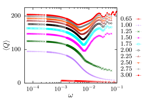
Figure 4: Averaged dynamical order parameter $\langle Q\rangle$ as a function of frequency $\omega$ (in log-scale) of the periodic force at various amplitudes $G$ for the DNA of length $N=128$.

III.2 Dynamical order parameter

The dynamical order parameter averaged over $10^{6}$ cycles, $\langle Q\rangle$, is plotted as a function of frequency $\omega$ (in log-scale) for the DNA of length $N=128$ at various force amplitudes $G$ in Fig. 4. For amplitude $G=0.65$, the maximum value of the periodic force is always less than the critical force (i.e., $g_{c}(1)=0.6778\dots$) needed to unzip the DNA at $T=1$, hence the DNA remains in the zipped state irrespective of the frequency of the periodic force. As discussed in SubsectionIIIA, the stationary state of the DNA is a zipped ($Z$) state when the force amplitude $G$ is 1.0 and 1.25, as could be seen by lower value of $\langle Q\rangle$ at higher frequencies. As at such frequencies, the DNA does not get time to respond to the change in the force value and effectively remains in its stationary state, which is a zipped configuration in this case. However, as the frequency decreases, the DNA starts responding to the periodic force and the value of $\langle Q\rangle$ increases and gets saturated. When the force amplitude is very high (i.e., $G=3$), the stationary state of the DNA is an unzipped ($U$) state as seen in the plot by the maximally allowed $\langle Q\rangle$ value at higher frequencies. As the frequency decreases, the value of $\langle Q\rangle$ shows oscillations before becoming constant at lower frequencies. The frequency at which there appears a larger dip in $\langle Q\rangle$ is exactly the same at which the hysteresis loop area, $A_{\rm loop}$, shows a maximum. The frequencies at which there are other minima in $\langle Q\rangle$ are also similar to the frequencies at which secondary maxima occur in $A_{\rm loop}$. Kapri2014

From the above discussion, we see that $\langle Q\rangle$ does not give any further useful information that has not already been obtained from the hysteresis loop area. Kapri2014 Therefore, we study the probability distributions, $P(Q)$, of the dynamical order parameter $Q$ defined by Eq. (3). We find that the allowed values of $Q$ do not follow a regular pattern and appears randomly. The distributions $P(Q)$ are obtained by binning $Q$ values acquired in $10^{6}$ cycles of the periodic force. The normalized distributions are shown in Figs. 3(d)-3(f) for the DNA of length $N=128$ at various frequencies $\pi/100$, $\pi/240$ and $\pi/1000$, for which the hysteresis loops are shown in Figs. 3(a)-3(c). At a higher frequency $\omega=\pi/100$ [Fig. 3(d)], the distributions $P(Q)$ for lower values of amplitudes $G=1.0$ and 1.2 are sharply peaked at lower values of $Q$ showing that the DNA is in the zipped ($Z$) phase. At an amplitude of $G=1.3$, the distribution $P(Q)$ becomes broader and spans both the zipped ($Z$) and dynamic ($D$) phases. On increasing the amplitude further (i.e., $G=1.5$), the distribution becomes narrower again with a peak for intermediate $Q$ values that lies in the dynamic $D$ phase. On increasing the amplitude further ($G=3$), the distribution is again sharply peaked at higher $Q$ values showing that the DNA is in the unzipped ($U$) phase. For a slightly lower frequency $\omega=\pi/240$ [Fig. 3(e)], the distributions are qualitatively similar to Fig. 3(d) but with a slightly more pronounced double peak structure for $G=1.3$. However, at much lower frequencies $\omega=\pi/1000$ [Fig. 3(f)], the distributions at all $G$ values become sharp. From these distributions, we can clearly see that the dsDNA could be taken from a zipped ($Z$) to an unzipped ($U$) state via a dynamic ($D$) state or vice versa at a constant frequency by changing the force amplitude. For higher frequencies, the distributions are very sensitive to the value of force amplitude $G$. There are regions where a small change in the value of $G$ could change a sharp distribution to a broader one. However, we could not get a three peak structure as seen in Langevin dynamics simulation study of shorter DNA hairpin under periodic force. Mishra2013

III.3 Correlation functions

In this section, we study the behavior of correlation functions of the extension between the end monomers of the two strands of the DNA and the dynamical order parameter $Q$ as a function of time.

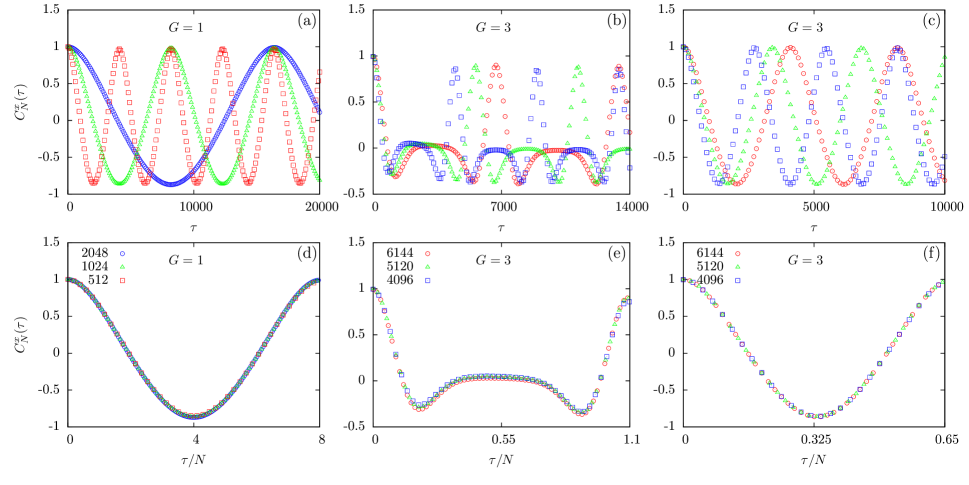
Figure 5: (Top) The correlation function of extension between the last monomers of two strands $C_{N}^{x}(\tau)$ as a function of $\tau$ for DNA of various lengths $N$ at force amplitudes (a) $G=1$ [(b) and (c)] $G=3$. (Bottom) The data for various $N$ collapse to a single scaling curve when $\langle x(t)x(0)\rangle$ is plotted with $\tau/N^{z}$ with dynamic exponent $z=1$.

III.3.1 Extension

In the presence of a periodic force, the DNA undergoes a transition from a zipped to an unzipped phase in each cycle. On a square lattice, with unit lattice spacing, the end-to-end displacement for the DNA having $N$ monomers can vary between $N\sqrt{2}$, for a completely stretched configuration, and $N$ for a zigzag configuration that has maximum entropy. The later configuration is taken by the DNA for lower force values where it is in the zipped state. However, for higher force values, the DNA is in a completely stretched unzipped state having maximum length. Therefore, in the presence of a periodic force, the length of the DNA fluctuates and have longitudinal modes. Furthermore, due to the geometry of the square lattice, the change in length of the DNA by flipping a monomer (i.e., along the $z$ axis) is exactly equal to the change in the separation of the end monomers (i.e., along the $x$ axis). Therefore, the length correlation function is exactly equal to the correlation function for the extension between the end monomers of the two strands.

We define the normalized time autocorrelation function of extension $x$ between the strands of DNA of length $N$ as

$$C^{x}_{N}(\tau)=\frac{\langle x(t)x(t+\tau)\rangle-\langle x(t)\rangle^{2}}{\langle x(t)^{2}\rangle-\langle x(t)\rangle^{2}}.$$ (5)

The correlation function of extension $C^{x}_{N}(\tau)$ as a function of time $\tau$ for the DNA of various lengths $N=1024$, 2048, and 4096 when it is subjected to a periodic force of frequency $\pi/4096$ at force amplitude $G=1$ is plotted in Fig. 2(b). A nice collapse for various lengths suggests that they have similar correlation, independent of DNA length, when subjected to a periodic force of same frequency. The extension between two times that differ by $\tau$ is maximally correlated (or anticorrelated), i.e., $C^{x}_{N}(\tau)=1\ (-1)$, when $\tau$ is an integral (half-integral) multiple of the time period of the oscillating force. In between, the correlation first decreases from a maximum to a minimum as $\tau$ increases from integral to half-integral multiple of the time period and then increases again to reach the maximum when $\tau$ increases from half-integral to integral multiple of the time period.

It is interesting to calculate the correlations of extension, $C_{N}^{x}(\tau)$, at different frequencies. In Figs. 5(a)-5(c), we have plotted $C^{x}_{N}(\tau)$ as function of time $\tau$ for the DNA of various lengths, $N$, at force amplitudes $G=1$ and $3$. The time required to unzip the DNA is proportional to its length. Therefore, on increasing the length of the DNA, we need to reduce the frequency of the applied force to keep the product $\omega N$ constant. By using a simple analysis for the condition of maximum hysteresis loop, it was found Kapri2014 that for $G=1$, the frequency $\omega$ of the applied force and the length $N$ of the DNA satisfy the expression $\omega=\pi/8N$. This relation is used to fix the frequency of various chain lengths in Fig. 5(a). For higher force amplitudes (e.g., $G=3$), it was found that the area of the hysteresis loop and the average dynamical order parameter show an oscillatory behavior. At the location of first minimum and the second maximum of the hysteresis loop area, the relation between $\omega$ and $N$ becomes $\omega=11\pi/12N$ and $\omega=3\pi/2N$, respectively. We use the above relations to fix the frequency of various chain lengths in our simulations. We have plotted $C^{x}_{N}(\tau)$ as a function of $\tau$ for $N=1024,2048$, and $4096$ in Figs. 5(b) and 5(c). When the above data for various $N$ are plotted as a function of $\tau/N$, we obtain an excellent collapse giving the dynamical exponent $z=1$ ($\tau\sim N^{z}$). The data collapse are plotted in Figs. 5(d)-5(f).

III.3.2 Dynamical order parameter

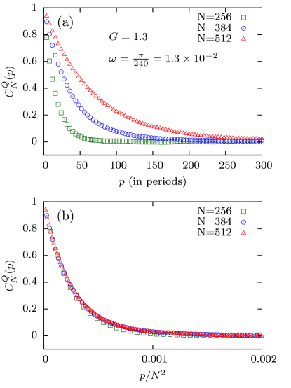
Figure 6: (a) Normalized autocorrelation function, $C_{N}^{Q}(p)$, of the order parameter $Q$ for the DNA of various lengths at force amplitude $G=1.3$ and frequency $\omega=\pi/240$ in units of MCS. (b) Collapse of data shown in (a).

We define the normalized time-autocorrelation function of the dynamical order parameter $Q$ for length $N$ as

$$C_{N}^{Q}(p)=\frac{\langle Q(i)Q(i+p)\rangle-\langle Q(i)\rangle^{2}}{\langle Q(i)^{2}\rangle-\langle Q(i)\rangle^{2}},$$ (6)

where $p$ represents the number of time periods. In Fig. 6(a), we have plotted $C_{N}^{Q}(p)$ as a function of $p$ for the DNA of lengths $N=256$, 384, and 512 when it is subjected to a periodic force of amplitude $G=1.3$ at frequency $\omega=\pi/240$. The increase in the correlation time with increasing system sizes gives evidence of critical slowing down of the system, providing support for the existence of a dynamical phase transition. When $C_{N}^{Q}(p)$ for various lengths are plotted as a function of $p/N^{2}$ (Fig. 6(b)), we get a nice collapse, implying that the number of time periods $p$ after which the order parameter $Q$ becomes completely uncorrelated depends on the system size as $p\sim N^{z_{p}}$, with dynamic exponent $z_{p}=2$.

III.4 Equilibrium curves

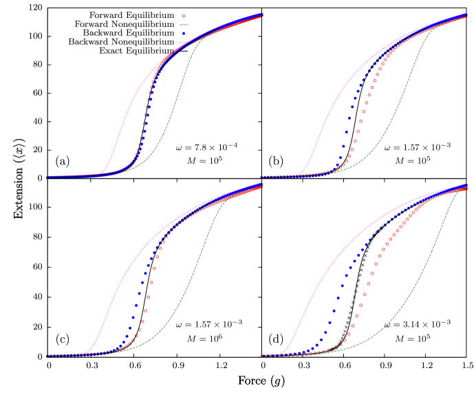
Figure 7: Force $g$ versus average extension $\langle x\rangle$ between the end monomers of the two strands of the DNA of length $N=64$ subjected to a periodic force of amplitude $G=1.5$ and frequencies $\omega=7.8\times 10^{-4}$ (a), $\omega=1.57\times 10^{-3}$ [(b) and (c)], and $\omega=3.14\times 10^{-3}$(d). In all the plots dashed (dotted) lines represent the forward (backward) nonequilibrium paths and open (closed) circles represent the equilibrium curves obtained by taking the weighted average from $M$ [$10^{6}$ in (c) and $10^{5}$ in (a), (b), and (d)] forward (backward) trajectories. The solid lines in all the plots are from the exact transfer matrix calculations. The symbol $\times$ in (d) at the transition region is obtained by using cubic spline interpolation scheme on the data up to $g=0.55$ from the forward, and the data beyond $g=0.80$ from the backward paths.

Kapri Kapri2012 has recently developed a procedure in the fixed force ensemble to obtain the equilibrium force-distance isotherms using nonequilibrium measurements. The scheme is similar to that of Hummer and Szabo HummerPNAS2001 in the fixed velocity ensemble which has been used successfully to obtain the zero force free energy on single molecule pulling experiments GuptaNPhys2011 . Both these procedures use the Jarzynski equality Jarzynski1997 — a work-energy theorem, which connects the thermodynamic free energy differences, $\Delta F$, between the two equilibrium states and the irreversible work done $W$ in taking the system from one equilibrium state to a nonequilibrium state with similar external conditions as that of other equilibrium state. The relation satisfied by $\Delta F$ and $W$ is $e^{\Delta F/k_{B}T}=\langle e^{-W/k_{B}T}\rangle$, where $k_{B}$ and $T$ are the Boltzmann constant and the absolute temperature, respectively. The angular bracket denotes average over all possible paths between the two states, which is dominated by rare paths. In the study of Kapri, Kapri2012 the two strands of the DNA are pulled apart by a force that is incremented by a constant rate from an initial value to some final value that lies above the phase boundary and then decreased back to the same initial value. For the present problem, the rate of change of force is not constant but we find that the same procedure could be used to obtain the equilibrium curves.

In our simulation, the time is incremented in discrete steps that is measured in units of MCS. Let $\tau_{p}$ denote the time period of the external force, we have $\omega=\pi/\tau_{p}$. Therefore, in each cycle, the force given by Eq.(1) also changes in discrete steps as

$$g_{k}=G|\sin(k\pi/\tau_{p})|,$$ (7)

where $k$ can take integer values $0,1,\dots\tau_{p}$. In the first half of the cycle ($k=0,\dots\tau_{p}/2$), the force $g_{k}$ changes from the minimum value $g_{k}=0$ to the maximum value $g_{k}=G$. We identify this as the forward path, and in the second half of the cycle $k=\tau_{p}/2+1,\dots\tau_{p}$ the force changes from $G$ to $0$ and is identify as the backward path.

Let $i$ and $k$ represent the indices for the cycle and the force, respectively. The irreversible work done over the $i$th cycle is given by

$$W_{ik}=-\sum_{j=0}^{k}(g_{j+1}-g_{j})x_{ij},$$ (8)

where, $x_{ij}$ is the extension between the end monomers of the dsDNA during $i$th cycle at force value $g_{j}$. By using $\exp(-\beta W_{ik})$ as the weight for path $i$, the equilibrium separation between the end monomers of the dsDNA, $x_{k}^{\rm eq}$, at force $g_{k}$ can then be obtained by SadhukhanJPA2010

$$x_{k}^{\rm eq}=\frac{\sum_{i=1}^{M}x_{ik}\exp\left(-\beta W_{ik}\right)}{\sum_{i=1}^{M}\exp\left(-\beta W_{ik}\right)}.$$ (9)

We use multiple histogram technique FerrenbergPRL1989 to approximate the density of states which then can be used to estimate the equilibrium separation $x_{k}^{\rm eq}$. To achieve this, we first build up the histogram $H_{k}(x)$ at each force value $g_{k}$. If the extension at $i$th cycle is $x$, the corresponding histogram value is incremented by $\exp(-\beta W_{ik})$

$$H_{k}(x)=\sum_{i=1}^{M}e^{-\beta W_{ik}}\delta_{x,x_{i}},\$$ (10)

where $\delta_{x,x_{i}}=1$ if $x=x_{i}$, and zero otherwise. At each force value $g_{k}$, the partition function $\mathcal{Z}_{k}$, obtained by using multiple histogram technique, FerrenbergPRL1989 is

$$\mathcal{Z}_{k}=\sum_{x}\rho(x)e^{\beta g_{k}x},$$ (11)

where the density of states, $\rho(x)$, is given by

$$\rho(x)=\left.\sum_{j}\frac{H_{j}(x)}{\mathcal{Z}_{j}}\middle/\sum_{j}\frac{e^{\beta g_{j}x}}{\mathcal{Z}_{j}}\right..$$ (12)

These equations need to be evaluated self consistently till they converge. The equilibrium separation $x_{k}^{\rm eq}$ at force value $g_{k}$ is then calculated by using the density of states $\rho(x)$ as

$$x_{k}^{\rm eq}=\frac{1}{\mathcal{Z}_{k}}\sum_{x}x\rho(x)e^{\beta g_{k}x}.$$ (13)

In Fig. 7, we have shown the force $g$, versus extension $\langle x\rangle$ curves for the DNA of length $N=64$ at force amplitude $G=1.5$ and three different frequencies $\omega=7.8\times 10^{-4}$, $1.57\times 10^{-3}$, and $3.14\times 10^{-3}$. At these frequencies, the dsDNA gets enough time to relax so it is in a completely unzipped phase at the maximum force value $g=1.5$ and in a completely zipped phase when the force value becomes zero. Therefore, we can use both the forward and the backward paths to calculate the equilibrium extension between the end monomers of the two strands. In these plots, the averaged nonequilibrium forward (backward) paths are shown by dashed (dotted) lines. The equilibrium curve is shown by a solid line. Thanks to the directed nature of the model, we could write a recursion relation for the partition function which could be solved numerically using the exact transfer matrix technique to obtain the partition function of DNA of length $N$ and the equilibrium force-distance isotherm. Kapri2012 This allows us to compare the results from our procedure to the exact result. The forward (backward) equilibrium extensions obtained by using the above procedure are shown by unfilled (filled) circles. Figure 7(a) shows the results for the frequency $\omega=7.8\times 10^{-4}$. At this frequency, the external force acting on the end monomers of the DNA changes slowly. The DNA gets more time to relax and therefore the area of the hysteresis curve traced by the averaged forward and backward paths of cycles is small. The equilibrium curve obtained by using the above procedure on $M=10^{5}$ forward and backward paths matches excellently with the curve obtained by using the exact transfer matrix. In Fig. 7(b), the results are shown for frequency $\omega=1.57\times 10^{-3}$ that is twice the frequency used in Fig. 7(a). The DNA gets lesser time to relax and therefore the area of the hysteresis curve increases. On using the above procedure for $M=10^{5}$ cycles we get the equilibrium curves that match with the exact equilibrium curve at lower and higher force values but not in the intermediate region where the transition takes place. This is due to the poor statistics in the transition region. However, if the number of cycles over which the histograms are taken are increased we get better statistics and the equilibrium curves obtained by using the forward and the backward paths will tend to coincide with the exact equilibrium curve, which can be seen in Fig. 7(c) where $M=10^{6}$ cycles are used keeping the frequency same as in Fig.7(b). If the frequency is doubled further (i.e., $\omega=3.14\times 10^{-3}$), the DNA gets much lesser time to relax and the area of the hysteresis loop increases. The equilibrium curves obtained by using the above procedure with $M=10^{5}$ cycles deviates from the actual equilibrium curve due to very poor statistics near the transition region. To get better statistics either one has to use more cycles, as mentioned earlier, or use special algorithms to generate rare samples, as these rare paths have the dominating contributions. However, on analyzing these curves closely, we find that the equilibrium curve obtained by using the forward (backward) path has good match with the exact equilibrium curve in the region that lies below (above) the critical force. This led to ask a question: can we combine the forward and the backward paths to obtain the equilibrium curve that matches with the exact curve even in the transition region? The answer to this question is in the affirmative. By using an interpolation scheme on the forward and the backward paths, we can obtain the equilibrium curve. To demonstrate this, we use data up to $g=0.55$ from the forward, and the data beyond $g=0.80$ from the backward paths with cubic spline interpolation scheme to obtain the equilibrium curve in the transition region. The result shown in Fig. 7(d) by the symbol $\times$ matches reasonably well with the exact curve obtained using transfer matrix in the transition region.

IV Conclusions

In this paper, we have reported the results of a periodically driven DNA using Monte Carlo simulations. We have obtained the average extension between the end monomers of the strands as a function of force, $\langle x(g)\rangle$, for various frequencies. If the frequencies are not small enough, the system does not get enough time to relax and $\langle x(g)\rangle$ shows hysteresis whose area gives the amount of energy dissipated to the system. It is observed that the steady state configuration of the DNA at higher frequencies and lower force amplitudes is a zipped ($Z$) state. At higher frequencies and higher force amplitudes, the steady state configuration of the DNA is two single strands that are far apart, i.e., the unzipped ($U$) state. We also obtained the average dynamic order parameter $\langle Q\rangle$ as a function of frequency and found that it does not reveal any new information that is not already known. Therefore, we obtained the probability distributions of $Q$ at different frequencies and force amplitudes. We observed that at a higher frequencies and for a small range of force amplitudes, the distribution $P(Q)$ is broad and spans both the zipped ($Z$) and the dynamic ($D$) phases. For lower and higher values of amplitudes, the probability distributions are sharply peaked that lie in one of the phases. We have obtained the autocorrelations of the extension between the end monomers of two strands, $C_{N}^{x}(t)$, as a function of time at different force amplitudes for various chain lengths. We found that the correlation $C_{N}^{x}(t)$ scales as $t/N$ at all amplitudes. We have also obtained the autocorrelation function of the dynamic order parameter, $C_{N}^{Q}(p)$, as a function of period number $p$ for force amplitude and frequency at which we have a broader distribution $P(Q)$ for various chain lengths. We observed that the quantity $Q$ appears randomly and its autocorrelation function behaves as $C_{N}^{Q}(p)\sim p/N^{2}$. Finally, we obtained the equilibrium force-extension curves at different frequencies by using the nonequilibrium work measurements. We find that it is possible to obtain the transition region with a good accuracy even for higher frequencies by interpolating the data of the forward and backward paths from the region where they are more accurate. In our opinion, the magnetic tweezers, which works in the fixed force ensemble, are the most suitable single molecule manipulation experimental technique to study the dynamical transitions in DNA unzipping with periodic forcing. The range of relevant frequencies depend on the length of the dsDNA and the force amplitude, which could be estimated by obtaining the time required in unzipping or rezipping of DNA at these force values. The procedure discussed in this paper would find application in obtaining the equilibrium curves in such experiments.

References

- (1) J. D. Watson et al., Molecular Biology of the Gene, 5 ed. (Pearson/Benjamin Cummings, Singapore, 2003).
- (2) S. B. Smith, Y. Cui and C. Bustamante, Science 271, 795 (1996).
- (3) M. D. Wang et. al., Biophys J. 72, 1335 (1997).
- (4) B. Essevaz-Roulet, U. Bockelmann and F. Heslot, Proc. Natl. Acad. Sci. USA 94, 11935 (1997).
- (5) U. Bockelmann et al., Biophys J. 82, 1537 (2002).
- (6) C. Danilowicz et. al., Phys. Rev. Lett. 93, 078101 (2004).
- (7) F. Ritort, J. Phys.: Condens. Matter 18, R531 (2006).
- (8) S. M. Bhattacharjee, J. Phys. A: Math. Gen 33, L423 (2000), arXiv:cond-mat/9912297.
- (9) D. K. Lubensky and D. R. Nelson, Phys. Rev. Lett. 85, 1572 (2000).
- (10) K. L. Sebastian, Phys. Rev. E 62, 1128 (2000).
- (11) D. Marenduzzo, A. Trovato and A. Maritan, Phys. Rev. E 64, 031901 (2001).
- (12) D. Marenduzzo, S. M. Bhattacharjee, A. Maritan, E. Orlandini and F. Seno, Phys. Rev. Lett. 88, 028102 (2001).
- (13) R. Kapri, S. M. Bhattacharjee, and F. Seno, Phys. Rev. Lett. 93, 248102 (2004).
- (14) R. Kapri and S. M. Bhattacharjee, J. Phys.: Condens. Mattter. 18, 215 (2006).
- (15) R. Kapri and S. M. Bhattacharjee, Phys. Rev. Lett. 98, 098101 (2007).
- (16) R. Kapri and S. M. Bhattacharjee, EPL 83, 68002 (2008).
- (17) R. Kapri, J. Chem. Phys. 130, 145105 (2009).
- (18) S. Kumar and M. S. Li, Phys. Rep. 486, 1 (2010).
- (19) M. Suman Kalyan and K. P. N. Murthy, Physica A 428, 38 (2015).
- (20) S. S. Velankar et al., Cell 97, 75 (1999).
- (21) K. Hatch, C. Danilowicz, V. Coljee and M. Prentiss, Phys. Rev. E 75, 051908 (2007).
- (22) R. W. Friddle, P. Podsiadlo, A. B. Artyukhin and A. Noy, J. Phys. Chem. C 112, 4986 (2008).
- (23) Z. Tshiprut and M. Urbakh, J. Chem. Phys. 130, 084703 (2009).
- (24) P. T. X. Li, C. Bustamante and I. Tinoco, Proc. Nat. Acad. Sci. 104, 7039 (2007).
- (25) D. Min et. al., Nature Communications 4, 1705 (2013).
- (26) G. Mishra, P. Sadhukhan, S. M. Bhattacharjee, and S. Kumar, Phys. Rev. E 87, 022718 (2013).
- (27) S. Kumar and G. Mishra, Phys. Rev. Lett. 110, 258102 (2013).
- (28) R. K. Mishra, G. Mishra, D. Giri and S. Kumar, J. Chem. Phys. 138, 244905 (2013).
- (29) S. Kumar, R. Kumar and W. Janke, Phys Rev E 93, 010402(R) (2016).
- (30) T. Pal and S. Kumar, EPL 121 18001 (2018).
- (31) R. Kapri, Phys. Rev. E 86, 041906 (2012).
- (32) R. Kapri, Phys. Rev. E 90, 062719 (2014).
- (33) B. K. Chakrabarti and M. Acharyya, Rev. Mod. Phys. 71, 847 (1999).
- (34) M. Doi and S. F. Edwards, The Theory of Polymer Dynamics (Oxford University Press, New York, 1986).
- (35) C. Jarzynski, Phys. Rev. Lett. 78, 2690 (1997).
- (36) G. Hummer and A. Szabo, Proc. Natl. Acad. Sci. U.S.A. 98, 3658 (2001).
- (37) A. N. Gupta et al., Nat. Phys. 7, 631 (2011).
- (38) P. Sadhukhan and S. M. Bhattacharjee, J. Phys. A 43, 245001 (2010).
- (39) A. M. Ferrenberg and R. H. Swendsen, Phys. Rev. Lett. 63, 1195 (1989).