Tracking Control by the Newton-Raphson Flow: Applications to Autonomous Vehicles

Abstract

This paper concerns applications of a recently-developed output-tracking technique to trajectory control of autonomous vehicles. The technique is based on three principles: Newton-Raphson flow for solving algebraic equations, output prediction, and controller speedup. Early applications of the technique, made to simple systems of an academic nature, were implemented by simple algorithms requiring modest computational efforts. In contrast, this paper tests it on commonly-used dynamic models to see if it can handle more complex control scenarios. Results are derived from simulations as well as a laboratory setting, and they indicate effective tracking convergence despite the simplicity of the control algorithm.

I Introduction

This paper considers a tracking problem where the output process of a continuous-time dynamical system has to match, within a given tolerance, a specified target curve. We address this problem by exploring a control technique that is based on the Newton-Raphson flow for dynamically tracking the solutions of time-dependent algebraic equations. The rationale behind the use of the Newton-Raphson flow is that it can have stabilizing effects on the closed-loop system, and endow the controller with effective tracking with modest computational efforts. The control technique has been proposed in [1] and tested on various academic examples in [1, 2]. The objective of this paper is to test it on more challenging control problems arising in applications to autonomous vehicles.

The control technique that will be presented may not be as general as existing nonlinear regulation techniques such as the Byrnes- Isidori regulator [3] and Khalil’s high-gain observers for output regulation [4], nor can we claim that it is more powerful. However, the effectiveness of these techniques is due to significant computational sophistication, like nonlinear inversions and the appropriate nonlinear normal form. On the other hand, the controller described in this paper is designed for simplicity and its implementation can be made by a fast algorithm. Regarding tracking applications to traffic control of autonomous vehicles, we do not claim that our technique outperforms extant methods based on Model Predictive Control (MPC) - the most common current approach to such applications. However, we perform the simulation testing on two specific problems that have been addressed by MPC techniques [5, 6], and the tracking-error results that we obtain are no worse. Also, our technique may be less computing-intensive than MPC (although no explicit comparison is made in the paper) because it requires no solutions of optimal control problems. In this, we do not claim that our technique is better than MPC; in fact, we think that it is not as general. We only argue that it deserves a further study for potential use in future applications.

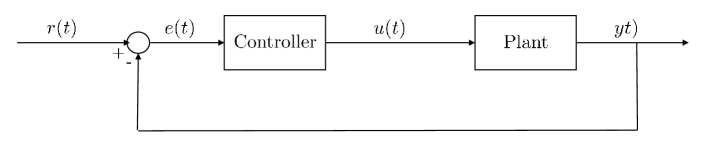
Figure 1: Basic control system.

To illustrate the Newton-Raphson flow, consider the continuous-time system in Fig. 1, where ${\{r(t):t\geq 0\}}$ is a given target curve in $R^{m}$, $\{u(t):t\geq 0\}$ is the control input to the plant, $\{y(t):t\geq 0\}$ is the system’s output, $e(t):=r(t)-y(t)$ and $\{e(t):t\geq 0\}$ is the error signal. We assume that the trajectories $\{r(t)\}$, $\{u(t)\}$ and $\{y(t)\}$, hence $\{e(t)\}$ are in the same Euclidean space, $R^{m}$. To highlight the salient features of the Newton-Raphson flow, suppose for a moment that the plant is a memoryless nonlinearity relating $u(t)$ to $y(t)$ by the equation

$$y(t)=g(u(t))$$ (1)

for a continuously-differentiable function $g:R^{m}\rightarrow R^{m}$. Define the controller by the following equation,

$$\dot{u}(t)=\left(\frac{\partial g}{\partial u}(u(t))\right)^{-1}\big{(}r(t)-g(u(t))\big{)},$$ (2)

assuming that the Jacobian matrix $\frac{\partial g}{\partial u}(u(t))$ is nonsingular for every $t\geq 0$. Since $y(t)=g(u(t))$, the controller can be viewed as a continuous-time flow of the Newton-Raphson method, tracking the solution of the time-dependent equation $g(u)=r(t)$; hence, we label it the “Newton-Raphson flow”.

We suggest the suitability of the Newton-Raphson flow to tracking applications in view of the fact that it is essentially an integrator, a key element in tracking control, albeit with a variable gain. To see this point, observe that ${e(t)=r(t)-y(t)}$; hence, Eq. (2) has the form $\dot{u}(t)=A(t)e(t)$ with $A(t):=(\frac{\partial g}{\partial u}(u(t)))^{-1}$. If $A(t)\equiv 1,$ then the controller would be the familiar integrator; as it stands, in Eq. (2), we can say that it is a variable gain integrator.

With the aforementioned particular gain $A(t)$, stability of the closed-loop system is hardly an issue. To see this, define the function $V:R^{m}\times R^{+}\rightarrow R^{+}$ by

$$V(u,t)=\frac{1}{2}||r(t)-g(u)||^{2}.$$ (3)

Then it is readily seen (e.g., [2]) that along trajectories in $u$, for every $t\geq 0$,

$$\dot{V}(t)\leq-||r(t)-g(u(t))||\big{(}||r(t)-g(u(t))||-||\dot{r}(t)||\big{)}.$$ (4)

If the curve $\{r(t)\}$ is continuously differentiable and bounded, define $\eta:=\sup\{||\dot{r}(t)||:t\geq 0\}$; then Eq. (3) implies that

$${\rm limsup}_{t\rightarrow\infty}||r(t)-g(u(t))||\leq\eta,$$ (5)

provided that the Jacobian matrix $\frac{\partial g}{\partial u}(u(t))$ is nonsingluar at every $t\geq 0$. This implies the boundedness of $\{u(t)\}$ and an upper bound, $\eta$, on the error $||r(t)-y(t)||$ (see Fig. 1). Note the special case where the target curve is a constant $r\in R^{m}$, then $V(u(t))$ is a Lyapunov function and $g(u(t))\rightarrow r$ as $t\rightarrow\infty$. In the general case of a nonconstant curve $\{r(t)\}$, the upper bound in the Right-Hand Side (RHS) of Eq. (5) can be reduced by speeding up the controller in the following way: multiply the RHS of Eq. (2) by a constant $\alpha>1$, thereby redefining the controller as

$$\dot{u}(t)=\alpha\left(\frac{\partial g}{\partial u}(u(t))\right)^{-1}\big{(}r(t)-g(u(t))\big{)};$$ (6)

then (see [2])

$${\rm limsup}_{t\rightarrow\infty}||r(t)-g(u(t))||\leq\eta/\alpha,$$ (7)

as long as the Jacobian $\frac{\partial g}{\partial u}(u(t))$ is nonsingular along the trajectory $\{u(t)\}$.

We stress the point that the boundedness and tracking properties of the controller require the sole assumption that the Jacobian $\frac{\partial g}{\partial u}(u(t))$ is nonsingular for every $t>0$. As a matter of fact, these properties are inherent in the direction defined by the Newton-Raphson flow. Now it is well known that, in its standard discrete-time setting, the Newton-Raphson method can be unstable ([7]), but this is due primarily to its step size and not its direction. In its flow setting the step size is infinitesimal, which seems to circumvent this stability issue.

If the plant is a dynamical system, then extensions of the controller, defined in Eq. (6) for memoryless systems, are not straightforward. For example, $y(t)$ is no longer a function only of $u(t),$ but rather of $\{u(\tau):\tau\leq t\}$; hence, it is unclear what $g(u(t))$ would mean. Moreover, as we shall see, stability of the closed-loop system cannot be taken for granted. We address these issues by defining the controller to be based on the following three principles: the Newton-Raphson flow, redefined in a suitable sense; an output predictor, which defines the time-dependent nonlinear equations that the controller attempts to solve; and a controller speedup, which aims at stabilizing the closed-loop system in addition to reducing the tracking error. The controller was defined in [1] and preliminary analysis and simulation results have been obtained in [1, 2] (surveyed below). As mentioned earlier, the main contributions of this paper are in the study of applications arising in autonomous vehicles through simulation and experimentation in a laboratory setting.

The rest of the paper is organized as follows. Sec. 2 recounts existing results and sets the stage for the later experiments. Sec. 3 describes simulation results, and Sec. 4 presents a laboratory experiment. Sec. 5 concludes the paper and suggests directions for future research.

II Problem Formulation and Previous Results

This section presents the controller’s definition as presented in [1], and recounts preliminary results in [1, 2].

Suppose that the plant subsystem in Fig. 1 is a dynamical system defined by the differential equation

$$\dot{x}(t)=f(x(t),u(t))$$ (8)

and the output equation

$$y(t)=h(x(t)),$$ (9)

where $x(t)\in R^{n}$ is the state variable, $u(t)\in R^{m}$ is the input at time $t$, and $y(t)\in R^{m}$ is the output at time $t$. The system evolves in the time-interval $t\in[0,\infty)$, and the initial condition for Eq. (8) is a given $x_{0}:=x(0)\in R^{n}$. The following assumption is made on the functions ${f:R^{n}\times R^{m}\rightarrow R^{n}}$ and ${h:R^{n}\rightarrow R^{m}}$:

Assumption 1

(i). The function $f:R^{n}\times R^{m}\rightarrow R^{n}$ is continuously differentiable, and for every compact set $\Gamma\subset R^{m}$ there exists $K>0$ such that, for every $x\in R^{n}$ and $u\in\Gamma$,

$$||f(x,u)||\leq K\big{(}||x||+1\big{)}.$$ (10)

(ii). The function $h:R^{n}\rightarrow R^{m}$ is continuously differentiable.

This assumption implies that for every bounded, piecewise-continuous input $\{u(t)\}$, and for every initial condition $x_{0}\in R^{n}$, Eq. (8) has a unique, continuous, piecewise continuously-differential solution $\{x(t)\}$ on $t\in[0,\infty)$.

In order to extend the controller from the above memoryless setting (Eq. (1)) to the current context of dynamical systems, we must have a way of expressing $y(t)$ as a function of $u(t)$ and perhaps other terms. To this end, and in order to ensure a suitable setting for the Newton-Raphson flow, we predict, at time $t$, the future output at time $t+T$ for a given $T>0$, and regard the predicted output as a function of $x(t)$ and $u(t)$. Specifically, define the predicted state trajectory in the time interval $\tau\in[t,t+T]$, denoted by $\xi(\tau)$, by the following differential equation,

$$\dot{\xi}(\tau)=f(\xi(\tau),u(t)),$$ (11)

with the initial condition $\xi(t)=x(t)$; then define the predicted output, $\tilde{y}(t+T)$, by

$$\tilde{y}(t+T)=h(\xi(t+T)).$$ (12)

Observe that $\tilde{y}(t)$ is a function of $x(t)$ and $u(t)$, and this functional dependence is denoted by

$$\tilde{y}(t+T)=g(x(t),u(t)).$$ (13)

The controller we define has the following form,

$$\dot{u}(t)=\alpha\left(\frac{\partial g}{\partial u}(x(t),u(t))\right)^{\!\!-1}\!\!\!\big{(}r(t+T)-g(x(t),u(t))\big{)},$$ (14)

and we note that this provides an extension of Eq. (6) as $g(x(t),u(t))$ depends on $u(t)$ and $x(t)$ as well. Eqs. (8), (9) and (14) together define the closed-loop system.

Generally, it is desirable to have the prediction horizon be as small as possible, since a smaller $T$ usually results in a smaller prediction error than a larger $T$, and this can translate into a smaller tracking error. Moreover, the effects of prediction errors on the tracking errors cannot be attenuated by speeding up the controller via a large $\alpha$ in Eq. (14), and hence, various applications may require a small prediction horizon $T$. However, initial analyses of simple examples, carried out in [1], revealed that, for a given $\alpha>0,$ there exists $T_{\alpha}>0$ such that the closed-loop system is stable for $T>T_{\alpha}$ and unstable for $T<T_{\alpha}$. In other words, for $T$ small enough, the system is unstable, which places a roadblock on the requirement of a small prediction horizon. However, it was also shown that $T_{\alpha}$ is monotone decreasing in $\alpha$, and

$$\lim_{\alpha\rightarrow\infty}T_{\alpha}=0,$$ (15)

which suggests the following practical implication: first, choose $T$ small enough to ensure a small prediction error, then choose $\alpha$ large enough to guarantee stability of the closed-loop system.

The aforementioned results were derived for particular simple systems, but they indicate that speeding up the controller may have two beneficial consequences: stabilizing the system and reducing the asymptotic tracking error as in Eq. (7). This was corroborated in [1, 2] by simulation experiments on various systems including an inverted pendulum, a platoon of mobile robots, and a network of mobile agents whose motion is coordinated by the graph Laplacian. While some of these control problems were challenging, the dynamic models and equations of motion of each of their constituent agents are quite simple, typically having the form of first-order or second-order linear systems. In contrast, as we said, in this paper we apply the control technique on systems with more complicated and realistic motion dynamics.

We point out that the key theoretical question concerns the derivation of verifiable conditions (necessary or sufficient) for the following property of the closed-loop system: for every $T>0,$ there exists $\bar{\alpha}>0$ such that, for every $\alpha>\bar{\alpha}$, the closed-loop system is stable. We label this property the $\alpha$-stability of the system. Thus far, it has been proved for the two-dimensional linear systems analyzed in [1], but an analysis in the general case is challenging due to the lack of closed-form expressions for $g(x,u)$. Simulation-based evidence suggests that generally, stability of the closed-loop system implies tracking in the sense of Eq. (7), and the derivation of verifiable sufficient conditions for various classes of systems is currently under way. Results of these theoretical investigations will be published elsewhere, while here we focus only on experimental verification in a particular application area.

III Simulation Results

This section presents results of simulation experiments for two problems taken from the literature on path tracking by autonomous vehicles [5, 6]. A key objective of this study is to test the tracking-control framework on system-models that are considerably more realistic and complex than the simple models used in the past [1, 2]. To this end we choose the bicycle model for the vehicles’ motion dynamics, which is often used in studies of control of autonomous vehicles (see, e.g., [8] and references therein). We adopt the dynamic model presented in [8, 6], and summarize it in the following paragraphs.

The state of the bicycle-model system is given by
${x=(z_{1},z_{2},v_{\ell},v_{n},\psi,\dot{\psi})^{\top}}$, where $z_{1}$ and $z_{2}$ are the planar coordinates of the center of gravity of the vehicle, $v_{\ell}$ is the longitudinal velocity, $v_{n}$ is the lateral velocity, $\psi$ is the vehicle’s heading and $\dot{\psi}$ is its angular velocity. The control input to the bicycle model is ${u=(a_{\ell},\delta_{f})^{\top}}$, where $a_{\ell}$ is the longitudinal acceleration, and $\delta_{f}$ is the front-wheel steering angle. For clarification, an illustration of the bicycle model is included in Fig. 2.

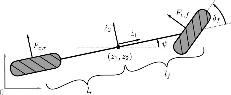
Figure 2: Dynamic bicycle model

Referring to the notation used in the previous section and especially to Eqs. (8) and (9), the state equation of the system is defined by the following equations:

$$\dot{z}_{1} =v_{\ell}\cos\psi-v_{n}\sin\psi$$ (16)

$$\dot{z}_{2} =v_{\ell}\sin\psi+v_{n}\cos\psi$$ (17)

$$\dot{v}_{\ell} =\dot{\psi}v_{n}+a_{\ell}$$ (18)

$$\dot{v}_{n} =-\dot{\psi}v_{\ell}+{2}\left(F_{c,f}\cos\delta_{f}+F_{c,r}\right)/{m}$$ (19)

$$\ddot{\psi} ={2}\left(l_{f}F_{c,f}\cos\delta_{f}-l_{r}F_{c,r}\right)/{I_{z}},$$ (20)

where $m$ is the mass of the vehicle, $l_{f}$ and $l_{r}$ are the respective distances of the front and back axles from the vehicle’s center of mass, $I_{z}$ is the yaw moment of inertia, and $F_{c,f}$ and $F_{c,r}$ are the lateral forces on the front and rear wheels. The forces $F_{c,f}$ and $F_{c,r}$ are approximated as:

$$F_{c,f}=C_{\alpha,f}\left(\delta_{f}-\tan^{-1}\left((v_{n}+l_{f}\dot{\psi})/v_{\ell}\right)\right)$$ (21)

$$F_{c,r}=-C_{\alpha,r}\tan^{-1}\left(({v_{n}-l_{r}\dot{\psi}})/{v_{\ell}}\right),$$ (22)

where $C_{\alpha,f}$ and $C_{\alpha,r}$ are the cornering stiffness of the front tire and rear tire.

For the purpose of output tracking we define the output by the planer coordinates of the center of gravity of the vehicle, namely $y=(z_{1},z_{2})^{\top}=Cx$, where

$$C=\left(\begin{array}[]{cccccc}1&0&0&0&0&0\\ 0&1&0&0&0&0\end{array}\right).$$ (23)

Instantiating the control equation (14), the controller has to compute the terms $g(x(t),u(t))$ and $\frac{\partial g}{\partial u}(x(t),u(t))$ in real time, at time $t$. By Eqs. (12) and (13), $g(x(t),u(t))=h(\xi(t+T))=C\xi(t+T)$, and $\xi(t+T)$ can be computed by numerical integration of the differential equation (11) in the interval $\tau\in[t,t+T]$, with the initial condition $\xi(t)=x(t)$. To this purpose we use the Forward-Euler method. As for the term $\frac{\partial g}{\partial u}(x(t),u(t))$, we observe that

$$\frac{\partial g}{\partial u}(x(t),u(t))=C\frac{\partial\xi(t+T)}{\partial u(t)}.$$ (24)

Moreover, by taking derivatives with respect to $u(t)$ in Eq. (11) the following equation for $\frac{\partial\xi(\tau)}{\partial u(t)}$ is obtained,

$$\frac{d}{d\tau}\frac{\partial\xi(\tau)}{\partial{u(t)}}=\frac{\partial f}{\partial\xi}(\xi(\tau),u(t))\frac{\partial\xi(\tau)}{\partial u(t)}+\frac{\partial f}{\partial u}(\xi(\tau),u(t)),$$ (25)

with the boundary condition $\frac{\partial\xi(t)}{\partial u(t)}=0$. This equation can be solved in the interval $\tau\in[t,t+T]$ by the forward Euler method, concurrently with Eq. (8), thereby yielding $\frac{\partial g}{\partial u}(x(t),u(t))$ via Eq. (24).

III-A Tracking of a closed curve

In this subsection we test the proposed controller on a bicycle model having to track a given closed curve. This problem was considered in [5] and we use the same parameters. However, we use a different model, as [5] uses a kinematic model whereas we use the dynamic bicycle model described above. The parameters of the problem are: $m=1,587~{}kg$, $I_{z}=2,315.3~{}kg~{}m^{2}$, $l_{f}=1.218~{}m$, $l_{r}=1.628~{}m$, and $C_{\alpha,f}=C_{\alpha,r}=35,000~{}N/rad$. The target track is depicted in Fig. 3. The target moves counterclockwise along the curve at a constant reference speed, and three simulation experiments were conducted for the following corresponding speeds: $15~{}km/h$, $25~{}km/h$ and $35~{}km/h$. The vehicle position is initialized on the track as indicated in Fig. 3 with the initial speed equal to the reference speed. The duration of each experiment is $100~{}s$. The parameters for the output-tracking controller are: the prediction horizon is $T=0.5~{}s$, the discretization time step for the predictor is $\Delta t=0.0025~{}s$, and the speedup coefficient in Eq. (14) is $\alpha=30$.

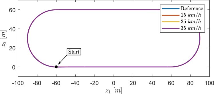
Figure 3: Closed-path tracking curve

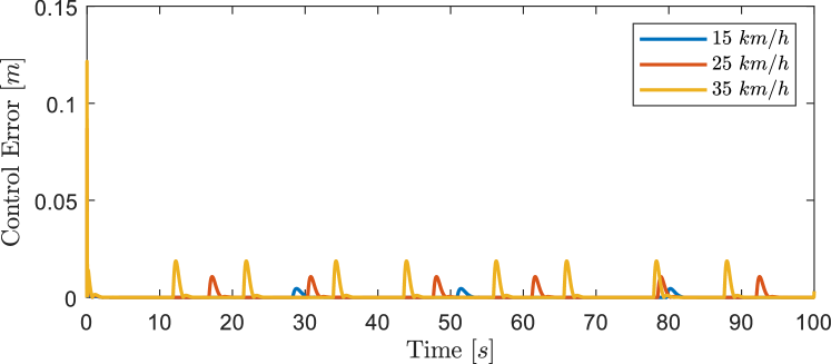
Figure 4: Closed path: control errors. Peak error (following an initial transient) is about $2~{}cm$.

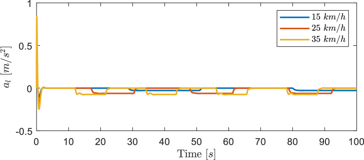
Figure 5: Closed path: longitudinal acceleration. Peak acceleration (following an initial transient) is under $0.1~{}m/s^{2}$.

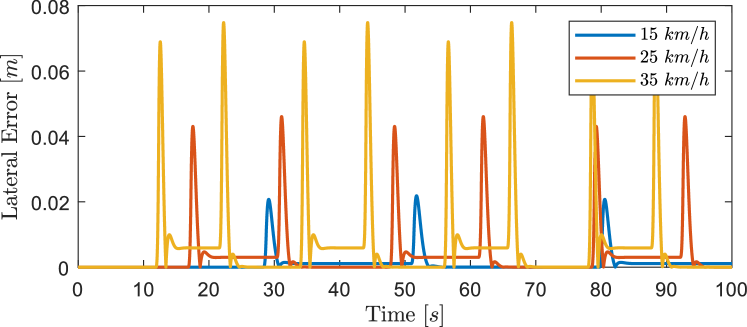
Figure 6: Closed path: lateral errors. Peak error is $8~{}cm$.

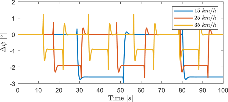
Figure 7: Closed path: heading errors. Peak error is under $3^{\circ}$.

Speed	Peak lateral error		Peak heading error
	Shivam 19	Zhou 17	Shivam 19	Zhou 17
$15~{}km/h$	$2~{}cm$	$36~{}cm$	$3^{\circ}$	$3.3^{\circ}$
$25~{}km/h$	$5~{}cm$	$23~{}cm$	$2.8^{\circ}$	$2.8^{\circ}$
$35~{}km/h$	$8~{}cm$	$17~{}cm$	$2.2^{\circ}$	$2.6^{\circ}$

TABLE I: Peak lateral and heading error for curve tracking

Fig. 3 shows the reference curve as well as the trajectories obtained from the three experiments, and the trajectories are barely distinguishable from the reference curve. Fig. 4 depicts the graphs of the control errors, which can serve to gauge the efficacy of the control algorithm.

With the exception of an initial transient, the peak control error is about $2~{}cm$, while counting the transients it is about $12.5~{}cm$. The small peaks in the control error correspond with turns on the reference curve which induce prediction errors. Fig. 5 shows the longitudinal acceleration of the trajectories which is under $0.1~{}m/s^{2}$ except for a transient where its peak is under $0.8~{}m/s^{2}$. Fig. 6 depicts the graphs of the lateral position errors, defined as the distance from the vehicle’s center of gravity to the target curve. We discern maximum errors of $2~{}cm$, $5~{}cm$, and $8~{}cm$ for the respective speeds of $15~{}km/h$, $25~{}km/h$, and $35~{}km/h$. The resulting heading errors are depicted in Fig. 7, and it is seen that the error does not exceed $3^{\circ}$. Ref. [5] also reports the lateral and heading (angular) errors obtained from its control algorithm. These and our simulation results are summarized in Table 1.

III-B Lane-change maneuver

The simulation performed in this subsection is applied to the same system and problem-parameters as described in [6]. We point out that [6] tested it by simulation and in a laboratory setting, while our results were obtained only from simulation. Note that the Pacejka tire model was used in [6]; however, in the range of operation the lateral forces are similar to those given by Eqs. (21)-(22).

The parameters of the vehicle are $m=2,050~{}kg$, $I_{z}=3,344~{}kg~{}m^{2}$, $l_{f}=1.105~{}m$, $l_{r}=1.738~{}m$, $C_{\alpha,f}=57500~{}N/rad$, and $C_{\alpha,r}=92500~{}N/rad$. The target curve, depicted in Fig. 8, is parameterized by the longitudinal position as given in [6]:

$$z_{2}=2.025\left(1+\tanh w_{1}\right)+2.85\left(1+\tanh w_{2}\right),$$ (26)

where $w_{1}=(2.4/25)(z_{1}-27.19)-1.2$ and $w_{2}=(2.4/21.95)(z_{1}-56.46)-1.2$. The target moves along the curve at a constant reference speed; simulation experiments were run for the following speeds: $10~{}m/s$, $15~{}m/s$, and $19~{}m/s$. In each simulation the vehicle starts at the origin at the reference speed. The duration of each experiment is $25~{}s$. The discretization step size for the numerical simulation is $0.01~{}s$. The controller prediction horizon is $T=0.5~{}s$, the discretization time step for the predictor is $\Delta t=0.001~{}s$ and the speedup coefficient is $\alpha=30$.

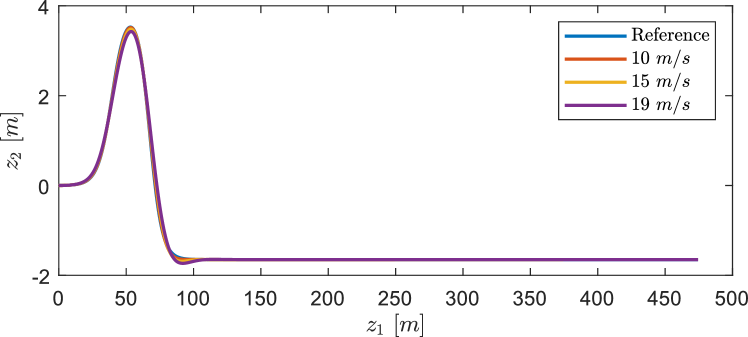
Figure 8: Lane-changing curve.

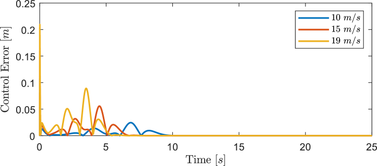
Figure 9: Lane changing: control errors. Peak error (following an initial transient) under $10~{}cm$.

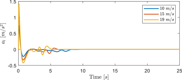
Figure 10: Lane changing: longitudinal acceleration. Peak acceleration (following an initial transient) is about $0.1~{}m/s^{2}$.

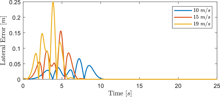
Figure 11: Lane changing: lateral errors. Peak error is $25~{}cm$.

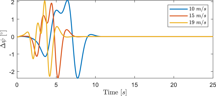
Figure 12: Lane changing: heading errors. Peak error is $2.5^{\circ}$.

Speed	Peak lateral error		Peak heading error
	Shivam 19	Falcone 07	Shivam 19	Falcone 07
$10~{}m/s$	$7~{}cm$	$96~{}cm$	$2.2^{\circ}$	$2.6^{\circ}$
$15~{}m/s$	$16~{}cm$	$125~{}cm$	$2.2^{\circ}$	$2.67^{\circ}$
$19~{}m/s$	$25~{}cm$	$158~{}cm$	$2.1^{\circ}$	$2.33^{\circ}$

TABLE II: Peak lateral and heading error for lane change

Fig. 8 shows the reference and the vehicle’s trajectories for the three experiments. The small tracking errors at about $z_{1}=52~{}m$ and $z_{1}=85~{}m$ correspond to sharp-direction changes in the target curve and likely are due to corresponding prediction errors. Fig. 9 depicts the control error, and is very small after the lane-change maneuver is completed. Fig. 10 shows the longitudinal acceleration of the vehicle, which has an initial transient peak of about $1.5~{}m/s^{2}$ for the $19~{}m/s$ reference speed, and is under $0.5~{}m/s^{2}$ thereafter. The lateral position error, depicted in Fig. 11, has peaks of $7~{}cm$, $16~{}cm$, $25~{}cm$ for the respective speeds of $10~{}m/s$, $15~{}m/s$ and $19~{}m/s$. The heading errors are plotted in Fig. 12 and have a maximum peak of approximately $2.5^{\circ}$.

Ref. [6] also provided the lateral errors and heading errors, and the peak values (for Controller B) as well as those obtained from our simulations are summarized in Table 2.

IV Experimental Results

This section presents the results of a laboratory experiment in which a platoon of four mobile robots follows a given path. The first robot tracks a point moving along the path, and each subsequent robot tracks a point on the path relative to the position of the preceding robot. The experiment used the differential-drive robots of the Robotarium, a remotely-accessible swarm-robotics testbed at Georgia Tech [9].

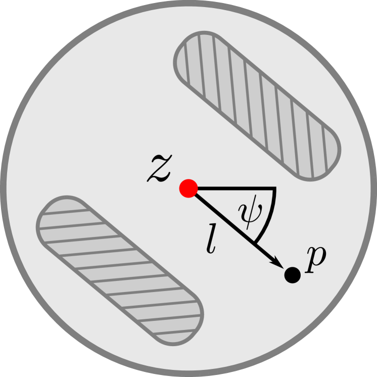
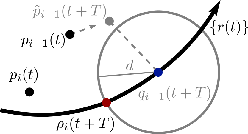
Figure 13: Left: Unicycle and kinematic point $p$ ahead of it. Right: An illustration of Algorithm 1 for robot $i.$

IV-A Robot modelling and control

The differential-drive robots of the Robotarium are modelled by unicycle dynamics given by the following equation

$$\begin{pmatrix}\dot{z}_{1}\\ \dot{z}_{2}\\ \dot{\psi}\end{pmatrix}=\begin{pmatrix}\cos\psi&0\\ \sin\psi&0\\ 0&1\end{pmatrix}\begin{pmatrix}v_{\ell}\\ \omega\end{pmatrix},$$ (27)

where $z:=(z_{1},z_{2})^{\top}$ is the position of the center of gravity of the robot, $\psi$ is its heading, $v_{\ell}$ is its longitudinal velocity, and $\omega$ is its angular velocity. In certain tracking applications one attempts to control $\{z(t)\}$ towards a curve $\{\bar{r}(t)\}$, and the control consists of the vector $(v_{\ell},\omega)^{\top}$. Here, to simplify the control of the unicycle, a transformation proposed by [10] is used to map the velocity vector of a kinematic point $p:=(p_{1},p_{2})^{\top}$ at a given distance $l$ ahead of the robot to the velocity vector $(v_{\ell},\omega)^{\top}$. This transformation is

$$\left(\begin{matrix}v_{\ell}\\ \omega\end{matrix}\right)=\left(\begin{matrix}\cos\psi&\sin\psi\\ -l^{-1}\sin\psi&l^{-1}\cos\psi\\ \end{matrix}\right)\left(\begin{matrix}\dot{p}_{1}\\ \dot{p}_{2}\end{matrix}\right);$$ (28)

see Fig. 13 for a visual aid. Under the mapping defined by Eq. (28), it is possible to control the robot by the state equation $\dot{p}=u$ with the input $u$, which simplifies the control law defined by Eq. (14) as compared to what it would be in the framework of Eq. (27).

In order to comply with the notation established in Sec. 2, define $x(t):=p(t)$, then Eqs. (8) and (9) have the form

$$\dot{x}(t)=u(t),~{}~{}~{}~{}~{}~{}~{}~{}y(t)=x(t).$$ (29)

Therefore, and by Eqs. (11)-(13),

$$g(x(t),u(t))=x(t)+Tu(t),$$ (30)

and hence $\frac{\partial g}{\partial u}(x(t),u(t))=T$. Consequently, Eq. (14) defining the control law becomes

$$\dot{u}(t)=\frac{\alpha}{T}\big{(}r(t+T)-x(t)-Tu(t)\big{)},$$ (31)

which does not require any numerical integration for computing $g(x(t),u(t))$ or $\frac{\partial g}{\partial u}(x(t),u(t))$.

It should be noted that while simplifying the control law, this procedure introduces a tracking error if the stated objective is to have $\{z(t)\}$, not $\{p(t)\}$ track $\{\bar{r}(t)\}$. However, this difficulty can be rectified by defining $\{r(t)\}$ as the trajectory of $\{p(t)\}$ if $\{z(t)\}\equiv\{\bar{p}(t)\}$; $p(t)$ can be computed as the point in the plane that is $l$ meters ahead of $\bar{p}(t)$ in the direction $\dot{p}(t)$. Using this transformation we consider, in the rest of this section, the control problem of having $\{p(t)\}$ track the curve $\{r(t)\}$.

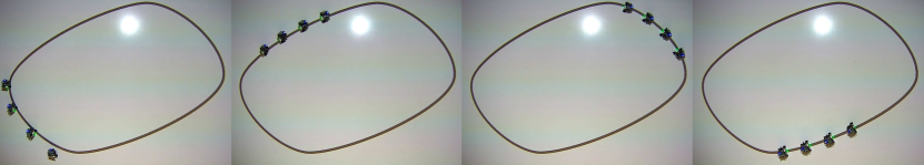
Figure 14: Stills from the Robotarium experiment. A platoon of four differential-drive robots moves along the path in a clockwise direction; the reference is displayed using an overhead projector. See [11] for a video.

IV-B Tracking problem definition

This subsection presents the tracking algorithm used in the experiment described below. Specifically, it details the procedure for determining the reference point that the kinematic point $p$ of each robot must track. The platoon is comprised of four robots indexed by $i=1,2,3,4$. The kinematic point associated with each robot is denoted by $p_{i}(t),$ and its control is achieved as described in the previous subsection.

The kinematic point of each robot $i=1,2,3,4$ tracks a point $\rho_{i}(t+T),$ which is on the reference path $\{r(t)\}$. The kinematic point of the first robot, the platoon leader, tracks the reference point $\rho_{1}(t+T):=r(\gamma(t+T)),$ where $\gamma>0$ is a scaling factor chosen to limit the rate at which $\rho_{1}(t+T)$ moves along the path. The need for such scaling stems from the fact that, if $\gamma=1$, the robots may be commanded to move at a higher speed than their physical limitations impose. The reference points for each of the kinematic points of the subsequent robots are determined as follows. Let $d>0$ be the target distance between $p_{i}$ and $p_{i-1}$, for $i=2,3,4$. At time $t$, let $\tilde{p}_{i-1}(t+T)$ be the predicted position of the point $p_{i-1}(t)$ at time $t+T$, and let $q_{i-1}(t+T)$ be the point on the curve $\{r(t)\}$ closest to $\tilde{p}_{i-1}(t+T)$. Let ${\tau_{i}(t+T):=\min_{\tau>t}\{||r(\tau)-q_{i}(t+T)||=d\}}$, and set the tracking-reference point to be ${\rho_{i}(t+T):=r(\tau_{i-1}(t+T))}.$ This procedure is formalized below by Algorithm 1 and illustrated in Fig. 13, below. The expression in Eq. (31) is applied to robot $i$ by replacing $u(t)$ with $u_{i}(t),$ $x(t)$ with $p_{i}(t),$ and $r(t+T)$ with $\rho_{i}(t+T)$.

Algorithm 1 Reference computation for robots $i=2,3,4$.

Inputs: $\{r(t)\}$ and $\tilde{p}_{i-1}(t+T)$
Output: $\rho_{i}(t+T)$.

$q_{i-1}(t+T)$ $\leftarrow$ the nearest point to $\tilde{p}_{i-1}(t+T)$ on $\{r(\cdot)\}$

$\tau_{i-1}(t+T)\leftarrow\min_{\tau>t}\{||r(\tau)-q_{i-1}(t+T)||=d\}$

$\rho_{i}(t+T)\leftarrow r(\tau_{i-1}(t+T))$

A few remarks are due. First, we implicitly assume that all of the quantities mentioned in Algorithm 1 are well defined, and expect this to be the case as long as $l\ll d,$ $d$ is smaller than the distance travelled by the robots in $T$ seconds, and the curvature of the path and its time-derivative are not too large; these considerations guide the choice of the reference path $\{r(t)\}$ as well the parameters $\gamma,$ $l,$ $d$, and $T$ for the experiments described in the next subsection. Second, Algorithm 1 can be performed by robots $i=2,3,4$ in a decentralized manner provided that has access to $\{r(t)\}$ and $\tilde{p}_{i-1}(t+T).$

IV-C Experimental Implementation

This subsection describes the laboratory experiment implemented in the Robotarium. The reference path, displayed on the testbed surface by an overhead projector, is shown in Fig. 14. The path is comprised of a concatenation of four third-order polynomials corresponding to the four sides of the path. The speed of the target point $r(t)$ is time-dependent, and its graph is depicted in Fig. 18. The following parameters are used: $l=0.08~{}m$, $d=0.25~{}m$, and the control-algorithm’s parameters are $\alpha=45$, $T=0.6~{}s,$ and the integration step size for computing the controls $u_{i}(t)$ is $\Delta t=0.033~{}s$. After some experimentation, we chose $\gamma=0.0455$.

The leftmost image of Fig. 14 shows the initial positions of the robots obtained by camera, not their corresponding kinematic points. From left to right, subsequent images show the counterclockwise progress of the robots along the path. Starting with the second image, near-equal distances between consecutive robots in the platoon is noted. A more detailed view of the motion of the robots can be seen from the video clip in [11].

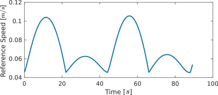
Figure 15: Experimental setting: reference speed

Figure 16: Experimental setting: trajectories of the kinematic points

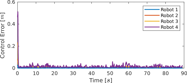
Figure 17: Experimental setting: control errors

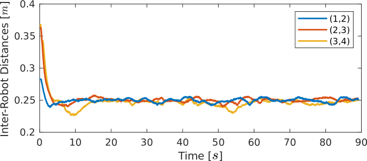
Figure 18: Experimental setting: inter-spacing between kinematic points of successive robots

Fig. 18 shows that the trajectories of the kinematic points $p_{i}(t)$, whose initial positions are indicated by the dots on the path. It is evident that the points $p_{i}(t)$ closely follow the target curve after initial transients. The resulting control errors, i.e., ${\|\rho_{i}(t+T)-\tilde{p}_{i}(t+T)\|}$ for $i=1,2,3,4$, are shown in Fig. 18. After ${t=1.4~{}s}$, the average control error for the four robots is approximately $5~{}mm$. Finally, examining the platoon, the three distances between successive kinematic points, $||p_{i}(t)-p_{i-1}(t)||$, $i=2,3,4$, are shown in Fig. 18, and they seem to approach the target distance of $25~{}cm$. The noted deviations of the last inter-spacing, $||p_{4}(t)-p_{3}(t)||$, from the $25~{}cm$ target occurs at about times $t=9.5~{}s$ and $t=54~{}s$, which correspond to the times of highest velocities as can be seen in Fig. 15.

V Conclusions

This paper presents experimental results on an output-tracking technique recently proposed by the authors. The technique is based on three principles: Newton-Raphson flow for the solutions of time-dependent algebraic equations, output prediction, and controller speedup. Past experiments, conducted on various systems with simple state-space models, exhibited fast tracking convergence. The main objective of this paper is to test the technique on more realistic models that are commonly used in the control of autonomous vehicles, in order to gauge its efficacy on more complicated control problems.

The paper describes results of experiments from simulation as well as a laboratory setting. For the simulation studies we chose two examples of curve-tracking problems from the literature, which use model-predictive control [5, 6]. Comparisons of the peak lateral error and peak heading error reported in these references, versus what was reported in this paper, indicate that our results are no worse. Therefore, and since the proposed technique does not solve differential equations and may be simpler than MPC, it may provide a framework for effective tracking control in future applications.

The lab experiments concern a platoon of mobile robots, where the objective is to control the inter-spacing between successive vehicles (robots) to a given reference distance. The results indicate convergence.

Current research includes theoretical as well as practical problems. The main theoretical question is how to identify conditions for stability of the closed-loop system, where a complicating factor is the fact that the controller’s function lacks a closed-form expression. A practical problem arises from the fact that currently the control technique is model-based. Current research addresses the use of learning algorithms so as to extend its scope to model-free environments.

References

- [1] Y. Wardi, C. Seatzu, M. Egerstedt, and I. Buckley, “Performance regulation and tracking via lookahead simulation: Preliminary results and validation,” in 56th IEEE Conf. on Decision and Control, Melbourne, Australia, December 12-15, 2017.
- [2] Y. Wardi, C. Seatzu, and M. Egerstedt, “Tracking control via variable-gain integrator and lookahead simulation: Application to leader-follower multiagent networks,” in Sixth IFAC Conference on Analysis and Design of Hybrid Systems (2018 ADHS)l, Oxford, the UK, July 11-13, 2018.
- [3] A. Isidori and C. Byrnes, “Output regulation of nonlinear systems,” IEEE Trans. Automat. Control, vol. 35, pp. 131–140, 1990.
- [4] H. Khalil, “On the design of robust servomechanisms for minimum phase nonlinear systems,” Proc. 37th IEEE Conf. Decision and Control, Tampa, FL, pp. 3075–3080, 1998.
- [5] H. Zhou, L. Guvenk, and Z. Liu, “Design and evaluation of path following controller based on mpc for autonomous vehicle,” in 36th Chinese Control Conference, Dailan, China, July 26-28, 2017.
- [6] P. Falcone, F. Borrelli, J. Asgari, H. Tseng, and D. Hrovat, “Predictive active steering control for autonomous vehicle systems,” IEEE Trans. Control Syst. Technology, vol. 15, pp. 566–5808, 2007.
- [7] P. Lancaster, “Error analysis for the newton-raphson method,” Numerische Mathematik, vol. 9, pp. 55–68, 1966.
- [8] J. Kong, M. Pfeiffer, G. Schildbach, and F. Borrelli, “Kinematic and dynamic vehicle models for autonomous driving control design,” in IEEE Intell. Veh. Symp. (IV), Seoul, Korea, June 28 – July 1, 2015.
- [9] D. Pickem, P. Glotfelter, L. Wang, M. Mote, A. Ames, E. Feron, and M. Egerstedt., “The Robotarium: A remotely accessible swarm robotics research testbed.” in IEEE Int. Conf. Robot. Autom., May 2017.
- [10] R. Olfati-Saber, “Near-identity diffeomorphisms and exponential epsilon-tracking and epsilon-stabilization of first-order nonholonomic SE(2) vehicles,” in IEEE Proc. Amer. Control Conf., vol. 6, 2002, pp. 4690–4695.
- [11] I. Buckley. (2018) https://www.youtube.com/watch?v=ejxMFJR_Sdc.