See far with TPNET: a Tile Processor and a CNN Symbiosis

Abstract

Throughout the evolution of the neural networks more specialized cells were added to the set of basic building blocks. These cells aim to improve training convergence, increase the overall performance, and reduce the number of required labels, all while preserving the expressive power of the universal network. Inspired by the partitioning of the human visual perception system between the eyes and the cerebral cortex, we present TPNET, which offloads universal and application-specific CNN from the bulk processing of the high resolution pixel data and performs the translation-variant image correction while delegating all non-linear decision making to the network.

In this work, we explore application of TPNET to 3D perception with a narrow-baseline (0.0001-0.0025) quad stereo camera and prove that a trained network provides a disparity prediction from the 2D phase correlation output by the Tile Processor (TP) that is twice as accurate as the prediction from a carefully hand-crafted algorithm. The TP in turn reduces the dimensions of the input features of the network and provides instrument-invariant and translation-invariant data, making real-time high resolution stereo 3D perception feasible and easing the requirement to have a complete end-to-end network.

1. Introduction

We consider our work to contribute the following:

• State-of-the-art narrow-baseline stereo camera which provides robust 3D measurements with 0.05 pixel accuracy and which is capable of operating at distances of hundreds to thousands meters (farther than automotive LIDAR and ToF cameras); and

• TPNET as a framework for partitioning the larger network into sensor-variant (“eyes”) and sensor-invariant (“brain”) subsystems, without sacrificing any of the capabilities of true end-to-end networks.

The recent development of vision perception systems is defined not only by advances in new network architectures but also by the emergence and general availability of new sensor technologies. The appearance of direct distance measurements with LIDAR and ToF cameras, which provide excellent range precision but low image plane resolution, triggered the development of the fusion of such sensor data with high resolution conventional images (Yang et al. [39], Park et al. [26], Gu et al. [13]).

The cellphone camera revolution contributed to the development of the Structure-from-Motion (SfM) 3D scene reconstruction. Recently, Torii et al. [36] suggested a two-stage network that first extracts features with VGG16 ($300\times 150\times 256$ tensors from $1600\times 1200$ images), then matches low-resoluton features to establish initial correspondences and improves the keypoints localization to a single-pixel resolution and builds 3D model from the N-best images. Other technological advances caused by the widespread adoption of cellphone cameras include methods for the enhancement of their images, such as motion blur elimination (Zhang et al. [42]) and Electronic Rolling Shutter (ERS) distortion correction with egomotion estimation from the video frames sequence (Forssén and Ringaby [10]) or even from a single frame by automatic feature extraction of four straight in real-world lines (Lao and Ait-Aider [18]).

The diversity of research in the field of vision-based 3D perception is handicapped by the limitations of publicly available datasets: Pingerra et al. [27] noticed that popular Middlebury and KITTI frameworks do not sufficiently treat local sub-pixel matching accuracy. We would add that such datasets are based on conventional binocular stereo and do not provide the data needed for deep subpixel calibration, effectively removing large application classes from consideration by machine learning researchers.

Most ML-based vision perception systems, even nominally end-to-end ones, start from the RGB images, usually rectified for compatibility with the translation-invariance nature of the CNN. The raw sensor data is neither rectified, no RGB, but rather a Bayer mosaic, normally consisting of a repeating $2\times 2$ (RG/GB) pixels pattern. Khamis et al. [17] achieved 1/30th of a pixel precision with an end-to-end network, that used synthetic data, same approach with KITTY 2015 [22] did not result in such precision. Bayer-to-RGB conversion is the most lossy part of the camera image capturing, and advanced networks like the one developed by Chen et al. [4] for low-light imaging bypass color conversion and use raw Bayer pixel data instead.

This leads to conflicting system requirements: on the one hand, the low-level image processing (color conversion, rectification) leads to loss of the important sensor data; on the other hand, resorting to the raw sensor data makes the whole system hardware-dependent and complicates the knowledge transfer and inference of the trained network.

We address these challenges by proposing a “network-friendly” system that adjusts the hardware, low-level processing and universal subnet to match existing DNN solutions. We developed a complete prototype system that outputs X3D (Brutzman and Daly [3]) scene models, but this is beyond the scope of this work. We focus here on the most under-explored part of the 3D vision perception that can be combined with and incorporated into other ML systems.

2. Related work

2.1 Long range stereo vision

Binocular stereo cameras for distance measurement and 3D scene reconstruction were very popular some 20 years ago and in 2002 Scharstein and Szeliski presented [32] taxonomy of dense two-frame stereo correspondence algorithms, at that time it did not distinguish between traditional and ML-based approaches. Since then these applications gradually lost their popularity for several reasons:

• direct active distance measurements with LIDAR and ToF cameras provide higher accuracy in most cases

• phone camera revolution made it easy to capture multiple views of the 3D objects to apply SfM processing.

There are still application areas where passive vision-based systems are preferable – in addition to obvious military ones where advertising yourself with the lasers is not acceptable, passive systems may have advantage for the longer range than practical for the automotive LIDAR scanners (over 200 meters) and for low power systems where illuminating environment with your own photons may be costly.

These considerations focus our work on the long range (>100 m), narrow-baseline cameras. For these cameras (Bayer mosaic color $2592\times 1936$, 2.2$\mu m$ pixels, FoV=$60\degree(h)\times 45\degree(v)$, baseline=258 mm) 100 m range corresponds to 5 pixel disparity, so the main challenge is to achieve accurate subpixel resolution that depends on:

• optical-mechanical stability of the system

• pixel noise

• image processing methods

Pingerra et al. [27] provided thorough comparison of multiple fractional pixel calculation methods and noticed that while results were varying by less than 1/30 pixel across all algorithms, the mean disparity error caused by a deviation in a camera calibration reached 1/10 of a pixel. We use thermally compensated sensor front ends with non-adjustable lenses relying on DoF of the small pixel cameras.

Nature of the various 3D capturing tasks involves processing of different number of pixels, influencing the disparity accuracy. The objects of interest may be small clusters of pixels, e.g. a distant flying drone, an edge of the foreground object or a textured (often poorly) surface. Small clusters case falls into the well investigated area of Particle Image Velocimetry (PIV) prone to the pixel-locking effect, described by Fincham and Spedding [9], Chen and Katz [5] proposed method of reducing this effect to under 0.01 pix for clusters of $4\times 4$ pixels and above, Westerweel [38] studied influence of the pixel geometry on correlation resolution. Pixel locking for stereo disparity may occur for larger patches: Shimizu and Okutomi [33] measured it by moving the target and then proposed compensation. Sabater et al. [31] considered theoretical limits of the disparity accuracy in the presence of pixel noise.

Phase correlation (PC) in the Frequency Domain (FD) is free of pixel locking: Hoge[15] used Singular Value Decomposition (SVD) for disparity from PC of the MRI images, Balci and Foroosh[1] developed plane fitting to the PC for satellite imagery. Morgan et al. [24] reported 0.022 pix RMSE for $32\times 32$ window model photos with fine texture using FD PC. Both methods (SVD and phase plane fitting) best work with large windows and small disparity variations, but direct feeding of the small window PC data to the trainable network may resolve ambiguity inherent to these methods.

We handle pixel locking in two ways: by fast converging iteration with lossless pre-shifting of the patches in FD, and then feed the network with that correlation data. Direct feeding of the FD representation to the network may be beneficial as it tends to concentrate important information in a small number of coefficients, but the pixel domain PC also has the same property to keep relevant data compact, we will try to concatenate both types of data.

Edges of the foreground objects are very important for stereo image matching as they correspond to photometric discontinuities and are the major contributors to the feature-based image matching, such as SIFT (Lowe [19]) and HOG descriptors used for human detection by Dalal and Triggs [7]. In the case of dense correspondence edges are handled by a separate term in SGM algorithm (Hirschmuller [14]) and its derivatives. SGM was developed for traditional implementation (including FPGA RTL) but it still remains efficient when combined with the network by Zbontar and LeCun [40].

Regardless of the image processing method, binocular stereo cameras are insensitive to the edges parallel to the epipolar lines. Commonly used systems with the two horizontally offset cameras cannot measure disparity of the horizontal linear features. We use quad camera system and process four directions for 2D PC as shown in Figure 1, these 45°orientations provide almost omnidirectional representations of the edges.

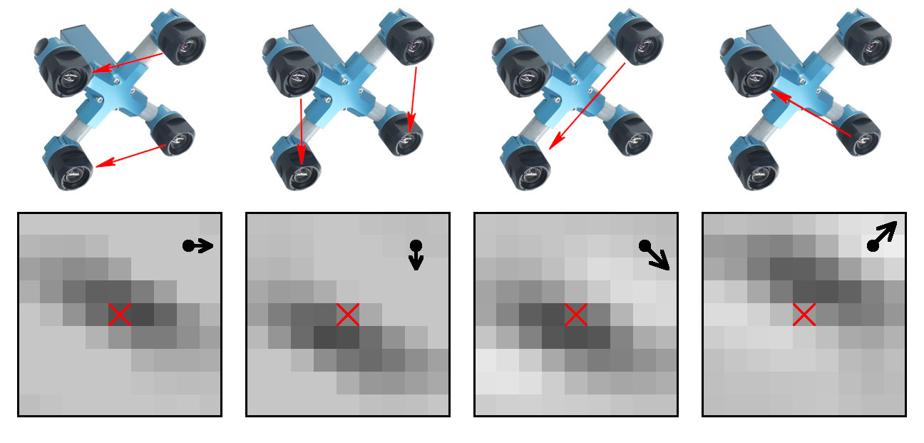
Figure 1: Quad stereo camera and 2D phase correlation (PC) samples between different image pairs.

2.2 FD and the neural networks

FD operations attract ML researches, one reason is that in FD computationally-intensive convolutions become trivial pointwise multiplications. Another – that the first CNN layers as visualized by deconvnet (Zeiler et al. [41]) exhibit Gabor-like patterns similar to FD representation and can potentially replace these layers with optimized modules.

Mathieu et al. [21] developed new CUDA FFT implementation and compared performance for variable image sizes (16-64) convolution with smaller $7\times 7$ kernels. Vasilache et al. [37] evaluated GPU implementations with NVIDIA cuFFT and their fbfft, reporting performance gains for the kernels above $3\times 3$. Brosch and Tam [2] studied two-layer convDBN trained in FD for 2D and 3D MRI images, achieving $200\times$ performance gain. Chen et al. [6] used Discrete Cosine Transform (DCT) instead of DFT followed by hash function to reduce width of the filters. Rippel and Adams [30] found that use of the 2D FD input to CNN followed by spectral pooling has advantages over max pooling in the pixel domain data. Zhao et al. [43] found that audio spectrograms improve performance from raw waveforms.

Figure 2: Bayer mosaic and lateral chromatic aberration. (a) Monochrome Point Spread Function (PSF). (b) Composite color PSF. (c) Bayer mosaic of the sensor (direction of aberration shown). (d) Distorted mosaic for chromatic aberration of (b).

In this work we use fixed-size ($16\times 16$ stride 8) Modified Complex Lapped Transform (MCLT) introduced by Princen et al. [29] and later applied to 2D image compression by De Queiroz and Tran [8] (we describe its details in Section 3.4). The focus of this work is to introduce an efficient interface between the low-level hardware-dependent image processing and translation-invariant CNN rather than to optimize convolutions in the network itself.

3. TPNET implementation

3.1 Best of the raw and the hardware-invariant

Most dense image matching 3D perception systems – both traditional and those based on DNN – try to determine each pixel’s disparity, typically with SGM [14] or its modifications. We split this task into a separate low spacial resolution disparity measurement, to be followed by fusion with the high-resolution RGBA images (where the alpha channel is calculated from the photometric differences between the images), similar to fusion for ToF cameras [13, 26, 39].

Replacing a single set of the raw images with multiple views of the same data resolves the conflicting requirements of the instrument and translation-invariance and the preservation of all of the relevant source data. Generally, the correction and rectification of image optical aberrations involves re-sampling that either requires up-sampling or adds quantization noise that jeopardizes subpixel accuracy. The correlation between the two tiles can be performed in the FD after performing the lossless phase rotation equivalent to the fractional pixel shift in the pixel domain. As the result, we can simultaneously obtain the RGBA data with pixel resolution and per-tile 2D correlation data for disparity measurements with full subpixel accuracy preserved. Both of these views provide instrument and translation-invariant data compatible with CNN, but neither of them can be derived from the other.

Similar to Chen et al. [4], we bypass Bayer to RGB conversion and use the raw data. The resolution of modern small pixel sensors is higher than that of the lenses, and aberrations in the off-center areas may even exceed the pixel pitch, invalidating assumption that red pixel is always located in the middle between four green ones (Figure 2). In this work, we process each color channel separately, apply individual aberration corrections, and merge results after the PC. Texture images merged from the four sensors using predicted disparity have Bayer-related artifacts attenuated from the single-camera artifacts, as the color patterns have random offsets. The final improvement of the texture images can be done with DNN (together with denoising and super-resolution), following the approaches of Gharbi et al. [11], Syu et al. [35] with modifications that consider multi-camera images of the same patches.

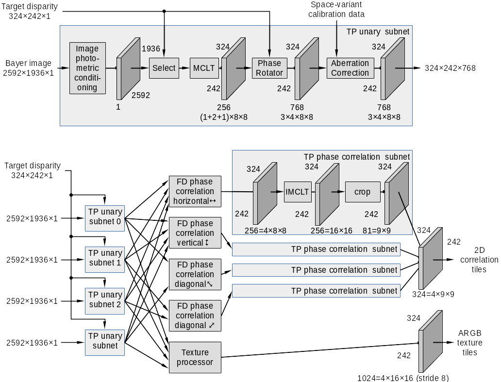
Figure 3: Tile Processor - a frequency domain pre-processor for the DNN

3.2 More non-collinear cameras

Use of the quad stereo camera instead of the conventional binocular layout extends SGM [14] approach to the camera design – we are not just calculating the disparity cost along multiple directions, but are rather measuring the disparity along multiple epipolar lines, allowing the downstream network to increase the weights of the correlations for the pairs orthogonal to the foreground object edge and ignore correlations produced by the background texture.

The increased number of image sensors as compared to the traditional binocular system is not expensive when it does not lead to an increase of the overall dimensions. Extra images will be reused to enhance the resolution of the combined image (Jeon et al. [16]) and to improve the S/N ratio of the sensors. Using more sensors when the parallax is compensated allows simultaneous HDR (Popovic et al. [28]) and multispectral 3D imaging (Neukum et al. [25]).

3.3 Frequency Domain (FD) processing

The initial TPNET implementation includes Tile Processor (TP), shown in Figure 3 and DNN (Figure 4) fed with the 2D correlation data from TP. TP performs the image conversion to the FD and the phase rotations (subpixel shifts), calculates the convolutions, PC and other FD operations, then converts the result arrays back to the pixel domain. We use fixed-size tiles that are large enough for deep subpixel disparity resolution; namely, tiles which are large enough to provide efficient pooling and reduction of disparity space image dimensions, but small enough to avoid scale and rotation mismatch. They are also sufficiently small so as to reduce the number of different disparity values sharing the same tile – usually just one or two for the edge of the foreground tile over the background.

3.4 Modified Complex Lapped Transform for FD

The tile receptive field is $16\times 16$ pixels, and, if applied to the full image with stride 8 (50% overlap in each direction), the operation is reversible due to the perfect reconstruction property of the MCLT [29, 20, 8]. Tiles do not have to be processed for the whole image, and each of them may have different “target disparity” (TD) that defines the selection of the image patches to be matched and the subpixel fraction shift to be applied before combining. The TD is analogous to eye convergence, but it is applied individually to each tile, not to the whole images.

MCLT implementation is based on Discrete Cosine Transform type IV (DCT-IV) and its sine counterpart DST-IV. MCLT is a generalization of MDCT - transform which is sufficient for compression but does not have the full convolution-multiplication property. For the single dimension, the forward transform MDCT normally uses the half-sine window function for the input data and “folds” $2N$ input sequence to an $N$-long ($N=8$ in our case) one. The subsequent DCT-IV transforms eight input values into eight outputs. When used for compression, these coefficients are subject to quantization and transmission to the decoder. The decoder performs an $N$-long inverse transform (in case of DCT-IV it is equal to the direct one), unfolds it to a $2N$-long sequence, and multiples it by the window function again (where the window satisfies the required Princen-Bradley condition [29]). The final step of the decoding would be to add together the individual $2N$-long sequences with overlap$N$, and without quantization the restored sequence will exactly match the initial one, losing only the first and the last $N$ of continuous samples.

For the full convolution-multiplication property to be valid, the complex-valued transform is needed, and for the single dimension the MCLT consists of a pair of MDCT and MDST, based on DCT-IV and DST-IV respectively, such that overlapping real-valued $2N$-long sequences are converted to pairs of $N$-long ones. Similarly, two dimensional $2N\times 2N$ tiles are converted to four (one for each variant of horizontal and vertical DCT-IV and DST-IV) $N\times N$ tiles. In case of $8\times 8$ transforms, the $16\times 16$ overlapping tiles are converted to $4\times 8\times 8$ real-valued tensors equivalent to twice larger $16\times 16$ DFT arrays with the same number of elements, but with complex instead of real values.

We modified MCLT algorithm to correctly handle translation-variant tile offsets by applying up to $\pm 0.5$ pix shifts to the original half-sine windows.

Our additional $3\times$ optimization is applied to the direct MCLT conversion of the Bayer mosaic images. Monochrome transformation of $16\times 16\times 1$ into $4\times 8\times 8$ tensor requires four $8\times 8$ DTT-IV ( “Trigonometric”, DTT = D{C,S}T) transforms. For the color Bayer mosaic tile of the same $16\times 16\times 1$ size, producing $3\times 4\times 8\times 8$ output requires equal number of DTT-IV operations (that is, four: 1 for red, 1 for blue and 2 for green), instead of the 12 needed for full RGB $16\times 16\times 3$ conversion.

3.5 Full 2D correlation instead of 1D epipolar

TP exploits the convolution-multiplication property for efficient implementation of the convolution and correlation. Rather than the conventional 1D correlation along the epipolar lines, we use full 2D correlation. Computationally, it does not require additional resources, as the 2D tiles are already available in FD after aberration correction, and the 2D correlation output for all pairs (Figure 1) provides the network with additional data about the edge direction; the relative importance of the pairs for the disparity measurement may be obtained from consolidating the data from several neighboring tiles, allowing the network to follow the linear features and to improve the S/N ratio in low textured areas. The 2D disparity vector is also used to correct the misalignment of the cameras. In addition to correlations between the tiles of the simultaneously captured images, the same TP can calculate motion vectors and measure optical flow from the consecutive frames of the camera.

3.6 Tile Processor pipeline

Incoming Bayer mosaic images (Figure 3) from each of the four sensors are first processed by identical channels that output FD tiles which preserve all the input data and thus may be converted back. In the current implementation, all of the required calibration data (such as the space-variant convolution kernels for aberration correction) are calculated with specially designed software and calibration setup. All the transformations are linear and differentiable with respect to both pixel values and calibration parameters, and they are immanent to the camera hardware, not to the specific application. This makes it possible to develop a trainable network to find the calibration kernels and the subcameras’ global intrinsic (such as focal length and radial distortion) and extrinsic (relative pose) parameters which is independent of the overall system application. Next, operations are performed for each tile independently which are parallelized according to the hardware capabilities (we developed RTL, CPU and GPU code, released as FLOSS). Tile coordinates are defined for the virtual camera located in the middle between the physical cameras. This virtual camera has radial distortion calculated as a best simultaneous fit for all the four actual cameras. The remaining deviations of each physical camera from the virtual one are considered aberrations and are treated the same way as chromatic and other aberrations by specifying centered deconvolution kernel and pixel offsets with fractional pixel resolution.

Each tile receives the target disparity value, uses extrinsic and distortion parameters to find nearest convolution kernel for each color, reads in that kernel, interpolates kernel center offset and calculates the full coordinates of each color component tile center and reads the corresponding image data from the $1936\times 2592$ array into combined $16\times 16$ buffer. The pixel window selection accommodates the integer part of the total pixel offset, while the fractional part is applied twice: first it modifies the nominally half-sine window function for MCLT, then after MCLT it is applied as a phase rotation in the FD, equivalent to the lossless fractional pixel shift. At this stage, the data does not have a real-valued pixel domain representation and so has to be processed in FD before the inverse transformation. It is point-wise multiplied by the calibration kernel, resulting in a $3\times 4\times 8\times 8$ tensor of corrected FD data for each tile, concluding the unary processing.

FD image tensors $242\times 324\times 3\times 4\times 8\times 8$ are used for 2D PC and texture processing. The 2D PC in the FD consists of pointwise complex multiplication, followed by weighed averaging between color channels and normalization. Then, each tile is converted to the pixel domain (using DCT-II/DST-II), and each $16\times 16$ output is cropped to the center $9\times 9$ shown in Figure 1.

The texture processor uses the same FD representations of corrected and shifted according to the specified disparity image tiles. They are combined and inverse-transformed to the pixel domain with the alpha-channel obtained from the pixel value differences between subcameras.

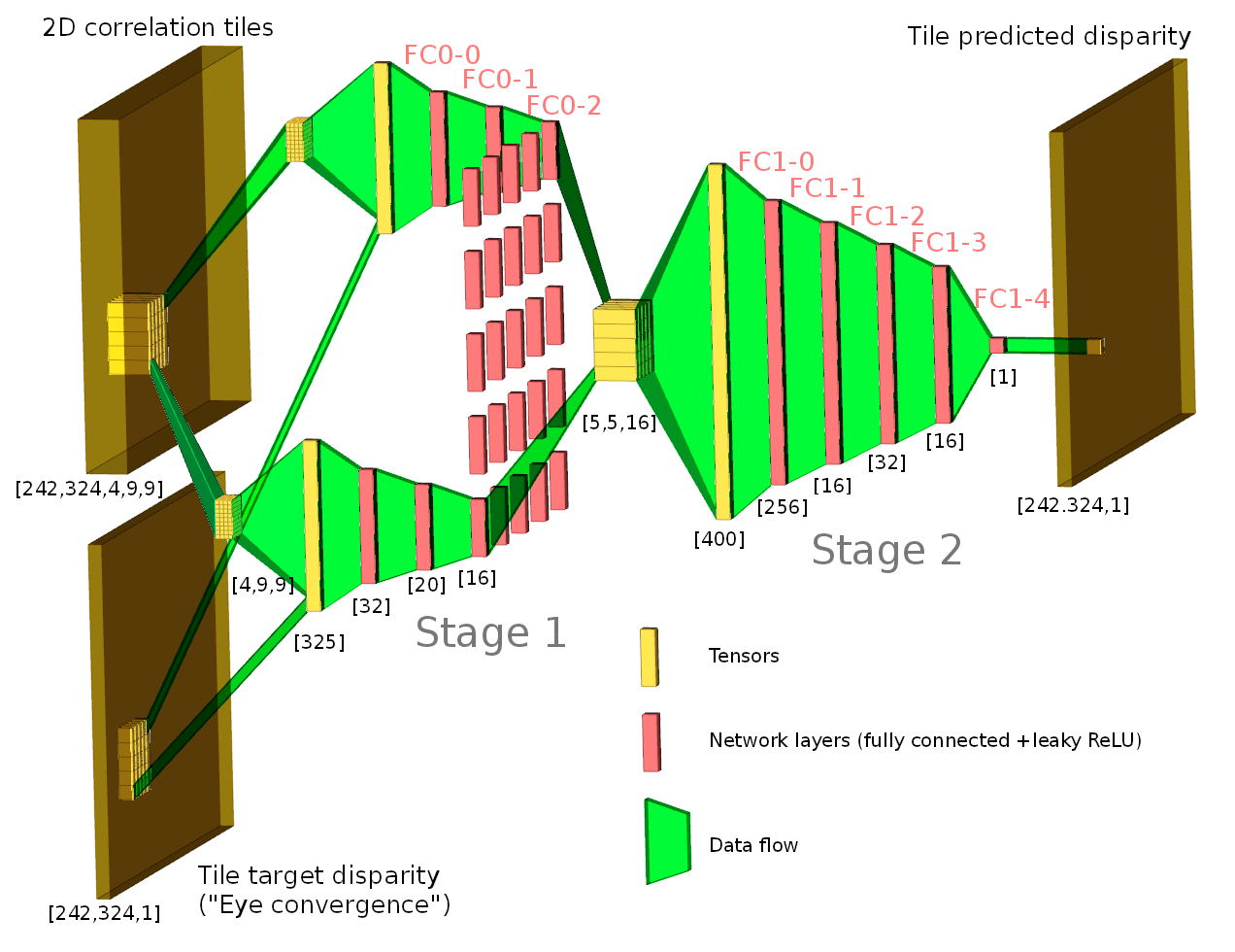
Figure 4: TPNET: initial implementation of the network.

3.7 Network part of the TPNET

The initial implementation of the TPNET is a simple feed-forward connection of the TP and a 2-stage network shown in Figure 4. The main goal of this implementation was to verify that we can significantly improve the results achieved by fitting a hand-crafted parametrized model with Levenberg–Marquardt algorithm (LMA). In the single-pass feed-forward implementation, each tile disparity is determined by LMA and then refined by re-running the tile correlation with updated target disparity until the step correction falls below the threshold.

The network consists of two stages: the first stage (3-4 fully connected layers with leaky ReLU activation for all but the last layer) operates on the correlation data from a single tile; the second convolutional (stride 1) stage receives the $242\times 324\times(16\ldots 64)$ tensor (stored in memory) generated by the first stage. For training, we used it as a 25-head Siamese network that outputs just a single disparity value for the center tile of $5\times 5$ tiles group; this allowed us to use mining of the input data for the “hard” cases (most of the tiles in the scene are almost fronto-parallell, as shown in Figure 7). Similar to the Siamese network for stereo matching by Zbontar and LeCun [40], in the separation between unary subnets and the second stage that unites them, the intermediate tensor has to be updated only when the corresponding input data changes. Unlike other networks, TPNET starts from 2D correlation data of multiple pre-shifted camera pairs and the stage 2 input features concatenation serves as a partially generalized 3D data exchange between neighbor tiles to improve disparity precision for the foreground edges that span multiple tiles and to handle low-textured areas by consolidating the correlation output from the groups of the neighboring tiles.

The first stage input features for a tile is a concatenation of the flattened $9\times 9\times 4$ correlation tensors (4 epipolar directions for each of the $9\times 9$ symmetrically cropped 2D PC cells) and a single target disparity (“eye convergence”) value that was used by the TP to pre-shift the image patches before correlating them. The output disparity is a sum of the target disparity and the residual disparity calculated from the correlation data, but the absolute disparity is still an important feature that modifies the network response to the same PC data. For the network output, we tried both the full disparity (sum of the target one and the residual) and just the residual with external summation. The last variant resulted in faster learning that we attributed to the observation that the network can still output reasonable differential result even without the target disparity knowledge. We used FC layers because while the correlation data is image-like it has strong translation asymmetry – the shape of the correlation data is influenced by the window function and random data in mismatched parts of the patches. PC of the real world objects is still a smooth function, and we successfully used a cost function term minimizing the Laplacian of the first layer weights for regularization.

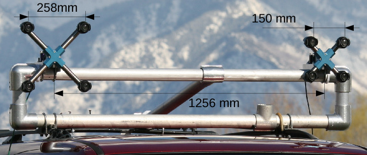
Figure 5: Experimental dual-quad stereo rig.

4. Experiments

Most of the trainable networks for stereo 3D perception use LIDAR data as ground truth (GT) for disparity prediction, including all that are based on the KITTY 2015 [22], such as recent work of Smolyanskiy et al. [34] that proves the advantages of stereo as compared to mono imaging even when combined with LIDAR direct depth measurements for autonomous vehicles. In our experiments, we were primarily interested in extremely long range 3D perception, with the narrow-baseline camera at several hundred to thousands of meters. The automotive LIDAR range is normally under 200 m, so we used a different setup, as shown in Figure 5. We mounted a frame through vibration isolators carrying a pair of quad cameras at a distance between their centers 4.87 times the tested quad camera baseline of 258 mm. The disparity accuracy of the composed camera (each of the 8 sensors has the same resolution and is paired with the identical lens) is expected to be proportionally higher than that of the single quad camera, and we used the distance data from the composite camera calculated with traditional software as GT. In the examples in Figures 7, 6 disparity values shown for the GT are scaled to match those of the 258 mm baseline camera for the same real world distances.

Over the course of the experiments, we found that the mechanical stability of the dual camera rig was lower than that of the individual cameras; consequently, we had to use field calibration (bundle adjustment of the relative pose) for each scene. We will improve GT accuracy by using SfM approach and ignoring moving objects during training.

We had 266 scenes processed and split the dataset in 80%/20% for training and testing. Instead of the full images, we used clusters of $5\times 5$ tiles corresponding to $48\times 48$ pixels image patches. The batches were shuffled to maintain the same representation of different disparity/confidence combinations. As most of the tile groups in the images belong to the smooth almost fronto-parallel surfaces, we performed mining for the rare cases of high disparity difference and increased the representation of such clusters while simultaneously lowering their weight in the cost function. The weights graph in Figure 7 illustrates the occurrence of the tile clusters as a function of the difference between the maximal and the minimal disparities.

When the same tile contains objects with disparity difference that is too small to be resolved in the PC output, the maximums merge and the fractional pixel argmax corresponds to nonexistent disparity between foreground and background objects. Example of this low-pass filter (LPF) effect is visible in Figure 6(c,d) on the right vertical edge of the building at $X=163,Y=100\ldots 110$. Training with just normalized to tile occurrence MSE cost for the available number of training samples did not remove the LPF from the predicted disparity output, so we added an additional term penalizing for the predicted disparity values between the GT value and that value mirrored around the average of 8 neighbor tiles. This cost function tweaking almost completely eliminated LPF effect in Figure 6(f).

Another cost modification is to improve convergence and delay overfitting. Stage 2 subnet shown in Figure 4 has a receptive field of $5\times 5$ Stage 1 outputs. Assuming that even a single center tile should be sufficient to provide a reasonable disparity estimate, we added two shared weights clones of Stage 2 - one with all but the center input tile masked out, and the other with the nine center tiles being non-zero. The same cost function was applied to all three outputs and the results were mixed with specified weights. For inference, only the original full Stage 2 subnet was kept.

Most image sets were captured during driving, so the precise matching is influenced by the rolling shutter (ERS). We have four sub-cameras synchronized and mechanically aligned to have parallel scan line directions matching (to $\pm 2$ pixels over the sensor width) and vertical WoI settings adjusted, making ERS caused by the camera egomotion (rotation) influence on disparity calculation negligible for objects at infinity (as they are captured simultaneously in all 4 channels). For the near objects, this effect is still small for the horizontal pairs, and it is possible to compensate it for the vertical ones by calculating the correction simultaneously with the 3D scene reconstruction. This correction is not yet implemented, and in this work we limited the maximal disparity to 5 pix that corresponds to 100 m range.

5. Results

Experimental results are presented in Figures 6 and 7. Figure 6 shows the GT and the predicted disparities for the far objects (680…2200 m range) captured by a forward-looking camera while driving in an urban environment, 6(b) shows the full FoV as GT confidence and marks the rectangular area enlarged in the other sub-images. Coordinate ticks designate tile horizontal and vertical indices. The building at (155,105) has disparity of 0.5 pix (1000 m), the faint one at (170,112) is the State Capitol at 2200 m from the camera. The full disparity calculated with the traditional algorithm (our best variant) is shown in 6(c), trained network predictions – in 6(e), and 6(d,f) contain the differences between the predicted disparities and the GT one.

Figure 7 contains the statistical results accumulated from the multiple test image sets. The horizontal axis represents the difference between the maximal and the minimal disparity in the $3\times 3$ group. The weights graph illustrates that most tiles are fronto-parallel and define the overall scene MSE. The RMSE graphs show the dependence of the prediction errors on the disparity variations around the tiles; ground truth LoG indicates non-flatness – it is the RMS of the difference between the tile and the mean of its eight neighbors.

The TPNET for training is implemented with Tensorflow/Python, and the inferred network is additionally tested with Tensorflow/Java. Processing all tiles in a frame with GeForce GTX 1050 Ti (compute capability 6.1, 4GB memory) Stage 1 takes 0.46 s, Stage 2 – 0.12 s run time, with the most time spent on CPU-to-GPU memory transfers. For the same GPU, the total processing time will be under 0.15 s when the network will be fed from the GPU implementation of the TP, bypassing large data transfers between the CPU and GPU memories. Separately tested GPU implementation of the TP took 0.087 s to process four of 5 Mpix images, including MCLT, aberration correction and IMCLT.

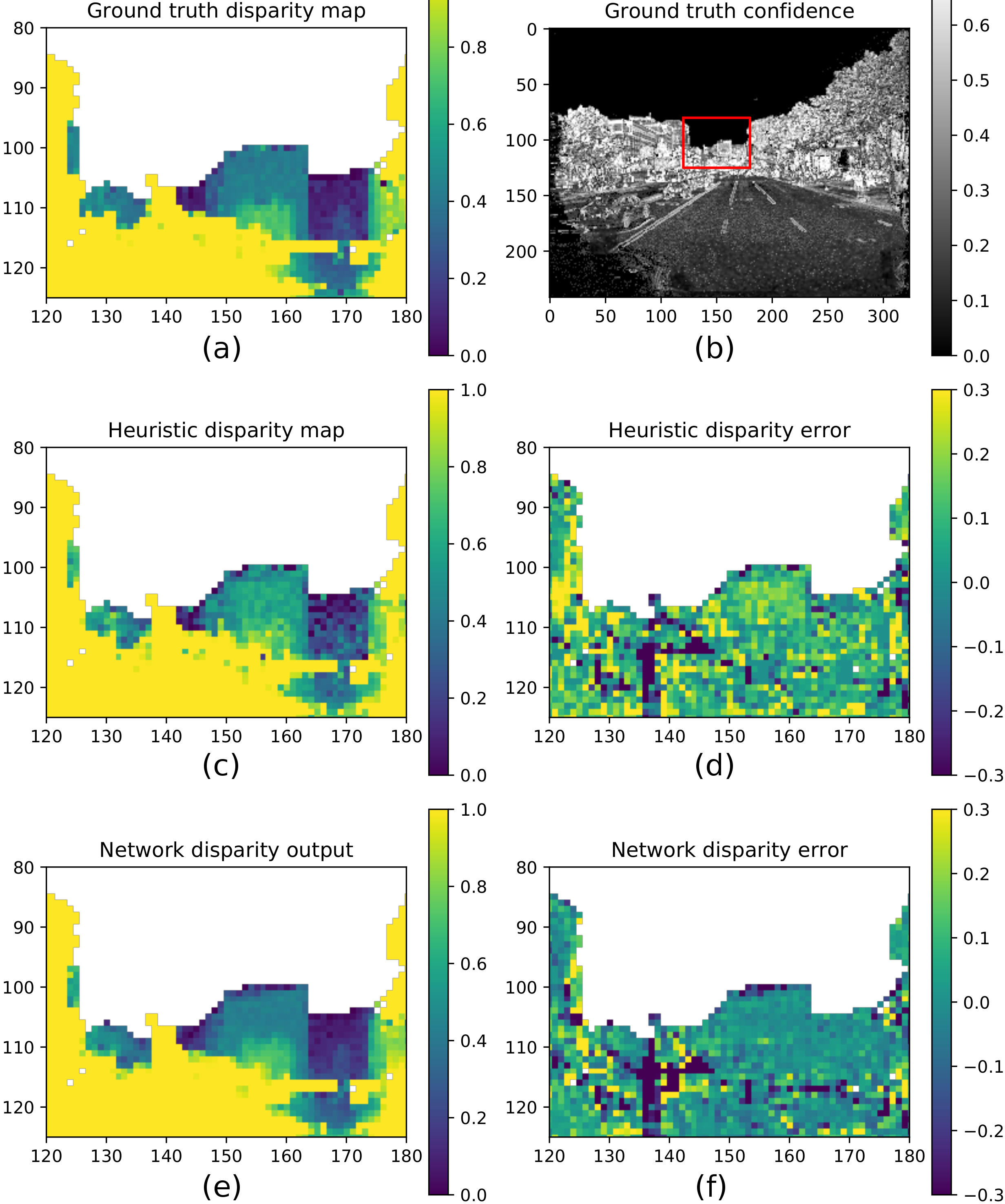
Figure 6: Disparity map comparison: TPNET vs heuristics. (a) Ground truth disparity. (b) Ground truth confidence and region of interest. (c) Absolute disparity calculated with traditional fitting. (d) Heuristic disparity error, difference between (c) and (a). (e) Network disparity prediction. (f) Network disparity error, difference between (e) and (a).

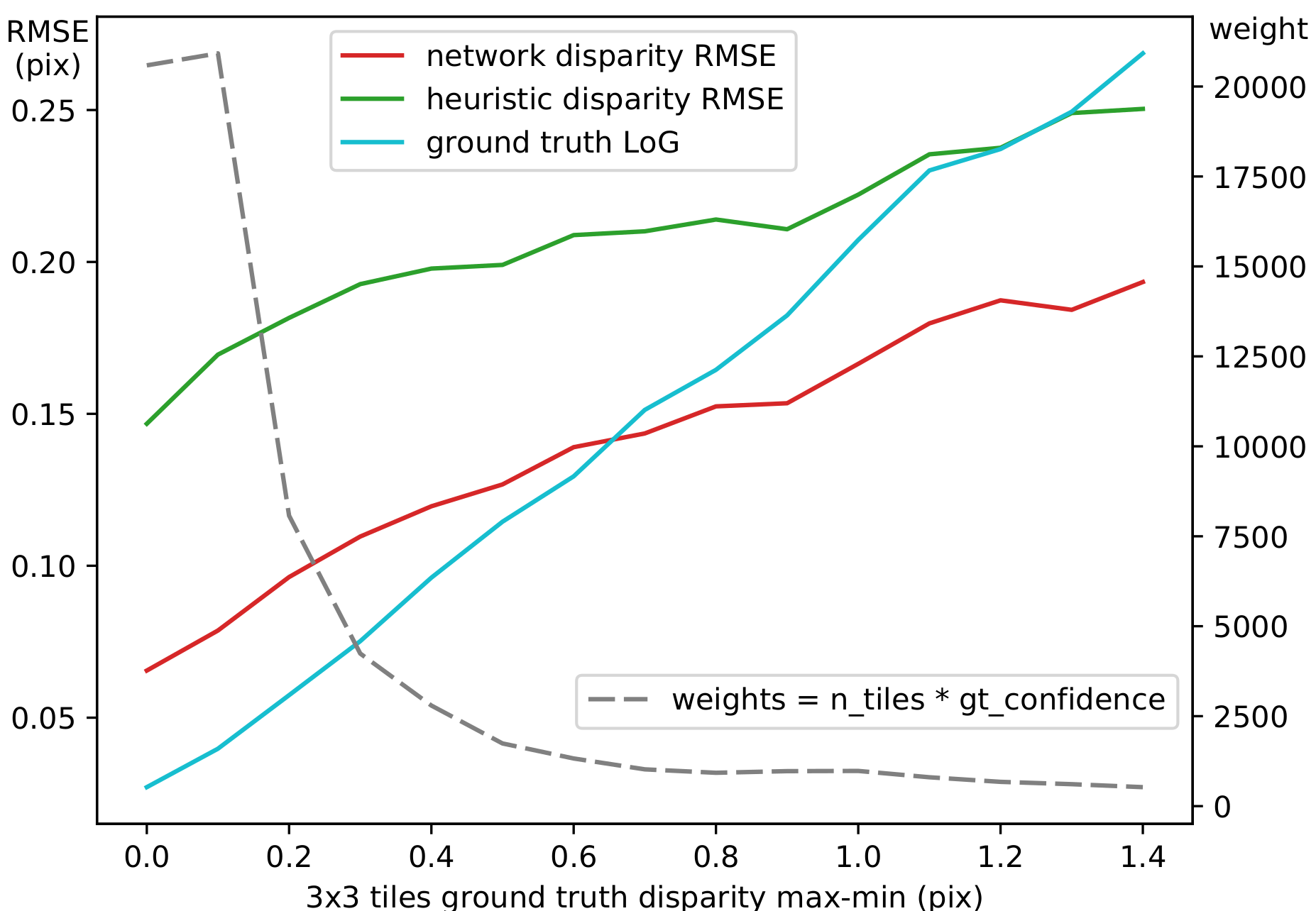
Figure 7: Disparity errors dependence on local ground truth disparity variations.

6. Discussion

Most of the work in the area of ML applications to image processing and 3D perception is shaped by the available datasets and COTS devices, such as cellphone cameras. Restricting attention to these datasets limits the diversity and reach of research in this field. Another problem that we target is poor interface between the hardware and low-level image processing on one side, and the advanced networks on the other. It pushes researchers to use full end-to-end approaches that lead to significant increases in the required labeled data and cause “brittleness” of the trained networks, requiring re-training for different hardware instances.

We introduce TPNET as an effective interface to partition the vision perception system into hardware-specific and hardware-invariant modules and prove that this combination is more efficient than implementing each part separately.

This initial TPNET has multiple limitations, as we were focusing on the new and untested components and assuming that it will be possible to later add known functionality, such as fusion of the multi-modal images [13, 26, 39]. Another limitation is that the TPNET still relies on non-ML code for the initial disparity estimation - this task can be better performed by the trainable networks. The same is true for the higher level task of 3D perception and reconstruction of the final model - it is also not converted from the over-complex heuristics to the ML. We plan to add feedback from the downstream semantic network to the TPNET for the fine-tuning of the PC processing. Segmentation such as described by Miclea and Nedevschi [23] (vegetation, poorly textured pavement, thin wires, vertical poles) may be applied to TPNET and used to modify the interpretation of the raw 2D correlation of the tile clusters.

The camera’s initial calibration currently depends on the special target pattern, and the field calibration uses traditional code. It is tempting to try a GAN-inspired (Goodfellow et al. [12]) adversarial game between the hardware-invariant subnet that detects discrepancies in the real world representation and the calibration network that adjusts the hardware-dependent parameters to avoid that detection.

7. Acknowledgments

We thank Tolga Tasdizen for his his suggestions on the network architecture and implementation.

References

- [1] M. Balci and H. Foroosh. Inferring motion from the rank constraint of the phase matrix. In Acoustics, Speech, and Signal Processing, 2005. Proceedings.(ICASSP’05). IEEE International Conference on, volume 2, pages ii–925. IEEE, 2005.
- [2] T. Brosch and R. Tam. Efficient training of convolutional deep belief networks in the frequency domain for application to high-resolution 2d and 3d images. Neural computation, 27(1):211–227, 2015.
- [3] D. Brutzman and L. Daly. X3D: extensible 3D graphics for Web authors. Elsevier, 2010.
- [4] C. Chen, Q. Chen, J. Xu, and V. Koltun. Learning to see in the dark. arXiv preprint arXiv:1805.01934, 2018.
- [5] J. Chen and J. Katz. Elimination of peak-locking error in piv analysis using the correlation mapping method. Measurement Science and Technology, 16(8):1605, 2005.
- [6] W. Chen, J. Wilson, S. Tyree, K. Q. Weinberger, and Y. Chen. Compressing convolutional neural networks in the frequency domain. In Proceedings of the 22nd ACM SIGKDD International Conference on Knowledge Discovery and Data Mining, pages 1475–1484. ACM, 2016.
- [7] N. Dalal and B. Triggs. Histograms of oriented gradients for human detection. In Computer Vision and Pattern Recognition, 2005. CVPR 2005. IEEE Computer Society Conference on, volume 1, pages 886–893. IEEE, 2005.
- [8] R. L. De Queiroz and T. D. Tran. Lapped transforms for image compression, 2001.
- [9] A. Fincham and G. Spedding. Low cost, high resolution dpiv for measurement of turbulent fluid flow. Experiments in Fluids, 23(6):449–462, 1997.
- [10] P.-E. Forssén and E. Ringaby. Rectifying rolling shutter video from hand-held devices. In Computer Vision and Pattern Recognition (CVPR), 2010 IEEE Conference on, pages 507–514. IEEE, 2010.
- [11] M. Gharbi, G. Chaurasia, S. Paris, and F. Durand. Deep joint demosaicking and denoising. ACM Transactions on Graphics (TOG), 35(6):191, 2016.
- [12] I. Goodfellow, J. Pouget-Abadie, M. Mirza, B. Xu, D. Warde-Farley, S. Ozair, A. Courville, and Y. Bengio. Generative adversarial nets. In Advances in neural information processing systems, pages 2672–2680, 2014.
- [13] S. Gu, W. Zuo, S. Guo, Y. Chen, C. Chen, and L. Zhang. Learning dynamic guidance for depth image enhancement. Analysis, 10(y2):2, 2017.
- [14] H. Hirschmuller. Accurate and efficient stereo processing by semi-global matching and mutual information. In Computer Vision and Pattern Recognition, 2005. CVPR 2005. IEEE Computer Society Conference on, volume 2, pages 807–814. IEEE, 2005.
- [15] W. S. Hoge. A subspace identification extension to the phase correlation method [mri application]. IEEE transactions on medical imaging, 22(2):277–280, 2003.
- [16] D. S. Jeon, S.-H. Baek, I. Choi, and M. H. Kim. Enhancing the spatial resolution of stereo images using a parallax prior. In Proceedings of the IEEE Conference on Computer Vision and Pattern Recognition, pages 1721–1730, 2018.
- [17] S. Khamis, S. Fanello, C. Rhemann, A. Kowdle, J. Valentin, and S. Izadi. Stereonet: Guided hierarchical refinement for real-time edge-aware depth prediction. arXiv preprint arXiv:1807.08865, 2018.
- [18] Y. Lao and O. Ait-Aider. A robust method for strong rolling shutter effects correction using lines with automatic feature selection. In Proceedings of the IEEE Conference on Computer Vision and Pattern Recognition, pages 4795–4803, 2018.
- [19] D. G. Lowe. Object recognition from local scale-invariant features. In Computer vision, 1999. The proceedings of the seventh IEEE international conference on, volume 2, pages 1150–1157. Ieee, 1999.
- [20] H. S. Malvar. Lapped transforms for efficient transform/subband coding. IEEE Transactions on Acoustics, Speech, and Signal Processing, 38(6):969–978, 1990.
- [21] M. Mathieu, M. Henaff, and Y. LeCun. Fast training of convolutional networks through ffts. arXiv preprint arXiv:1312.5851, 2013.
- [22] M. Menze and A. Geiger. Object scene flow for autonomous vehicles. In Conference on Computer Vision and Pattern Recognition (CVPR), 2015.
- [23] V.-C. Miclea and S. Nedevschi. Semantic segmentation-based stereo reconstruction with statistically improved long range accuracy. In Intelligent Vehicles Symposium (IV), 2017 IEEE, pages 1795–1802. IEEE, 2017.
- [24] G. L. K. Morgan, J. G. Liu, and H. Yan. Precise subpixel disparity measurement from very narrow baseline stereo. IEEE Transactions on Geoscience and Remote Sensing, 48(9):3424–3433, 2010.
- [25] G. Neukum, R. Jaumann, F. Scholten, and K. Gwinner. The high resolution stereo camera (hrsc): acquisition of multi-spectral 3d-data and photogrammetric processing. In International Conference on Space Optics—ICSO 2000, volume 10569, page 1056921. International Society for Optics and Photonics, 2017.
- [26] J. Park, H. Kim, Y.-W. Tai, M. S. Brown, and I. Kweon. High quality depth map upsampling for 3d-tof cameras. In Computer Vision (ICCV), 2011 IEEE International Conference on, pages 1623–1630. IEEE, 2011.
- [27] P. Pinggera, D. Pfeiffer, U. Franke, and R. Mester. Know your limits: Accuracy of long range stereoscopic object measurements in practice. In European Conference on Computer Vision, pages 96–111. Springer, 2014.
- [28] V. Popovic, K. Seyid, E. Pignat, Ö. Çogal, and Y. Leblebici. Multi-camera platform for panoramic real-time hdr video construction and rendering. Journal of Real-Time Image Processing, 12(4):697–708, 2016.
- [29] J. Princen, A. Johnson, and A. Bradley. Subband/transform coding using filter bank designs based on time domain aliasing cancellation. In Acoustics, Speech, and Signal Processing, IEEE International Conference on ICASSP’87., volume 12, pages 2161–2164. IEEE, 1987.
- [30] O. Rippel, J. Snoek, and R. P. Adams. Spectral representations for convolutional neural networks. In Advances in neural information processing systems, pages 2449–2457, 2015.
- [31] N. Sabater, J.-M. Morel, and A. Almansa. How accurate can block matches be in stereo vision? SIAM Journal on Imaging Sciences, 4(1):472–500, 2011.
- [32] D. Scharstein and R. Szeliski. A taxonomy and evaluation of dense two-frame stereo correspondence algorithms. International journal of computer vision, 47(1-3):7–42, 2002.
- [33] M. Shimizu and M. Okutomi. Sub-pixel estimation error cancellation on area-based matching. International Journal of Computer Vision, 63(3):207–224, 2005.
- [34] N. Smolyanskiy, A. Kamenev, and S. Birchfield. On the importance of stereo for accurate depth estimation: An efficient semi-supervised deep neural network approach. arXiv preprint arXiv:1803.09719, 2018.
- [35] N.-S. Syu, Y.-S. Chen, and Y.-Y. Chuang. Learning deep convolutional networks for demosaicing. arXiv preprint arXiv:1802.03769, 2018.
- [36] A. Torii, M. Okutomi, et al. Structure-from-motion using dense cnn features with keypoint relocalization. arXiv preprint arXiv:1805.03879, 2018.
- [37] N. Vasilache, J. Johnson, M. Mathieu, S. Chintala, S. Piantino, and Y. LeCun. Fast convolutional nets with fbfft: A gpu performance evaluation. arXiv preprint arXiv:1412.7580, 2014.
- [38] J. Westerweel. Effect of sensor geometry on the performance of piv interrogation. In Laser techniques applied to fluid mechanics, pages 37–55. Springer, 2000.
- [39] Q. Yang, R. Yang, J. Davis, and D. Nistér. Spatial-depth super resolution for range images. In Computer Vision and Pattern Recognition, 2007. CVPR’07. IEEE Conference on, pages 1–8. IEEE, 2007.
- [40] J. Zbontar and Y. LeCun. Computing the stereo matching cost with a convolutional neural network. In Proceedings of the IEEE conference on computer vision and pattern recognition, pages 1592–1599, 2015.
- [41] M. D. Zeiler, D. Krishnan, G. W. Taylor, and R. Fergus. Deconvolutional networks. In Computer Vision and Pattern Recognition, 2010. CVPR 2010. IEEE Computer Society Conference on. IEEE, 2010.
- [42] J. Zhang, J. Pan, W.-S. Lai, R. W. Lau, and M.-H. Yang. Learning fully convolutional networks for iterative non-blind deconvolution. In Computer Vision and Pattern Recognition Workshops (CVPRW), 2017 IEEE Computer Society Conference on, 2017.
- [43] H. Zhao, C. Gan, A. Rouditchenko, C. Vondrick, J. McDermott, and A. Torralba. The sound of pixels. arXiv preprint arXiv:1804.03160, 2018.