Neural Belief-Propagation Decoders for Quantum Error-Correcting Codes

Abstract

Belief-propagation (BP) decoders play a vital role in modern coding theory, but they are not suitable to decode quantum error-correcting codes because of a unique quantum feature called error degeneracy. Inspired by an exact mapping between BP and deep neural networks, we train neural BP decoders for quantum low-density parity-check (LDPC) codes with a loss function tailored to error degeneracy. Training substantially improves the performance of BP decoders for all families of codes we tested and may solve the degeneracy problem which plagues the decoding of quantum LDPC codes.

Statistical inference on a graph is an important paradigm in many areas of science, and equivalent heuristic algorithms have been developed by different communities, including the cavity method in statistical physics (Mezard et al., 1986) and the belief propagation (BP) algorithm in information science (Pearl, 1982). In the latter case, BP is the standard decoding algorithm for low-density parity-check (LDPC) codes (Gallager, 1962), which form the backbone of modern coding theory and are widely used in wireless communication (Richardson and Urbanke, 2008). With the growing interest for quantum technologies, quantum generalizations of LDPC codes have been proposed (MacKay et al., 2004; Tillich and Zemor, 2014; Leverrier et al., 2015), but BP was found to be inadequate for their decoding (Poulin and Chung, 2008) because of error degeneracy, a feature unique to quantum codes. Despite many improvements (Poulin and Chung, 2008; Wang et al., 2012; Babar et al., 2015) to BP, there is still no accurate decoding algorithm for general quantum LDPC codes. This contrast with statistical physics where the cavity method has been generalized to the quantum setting with some success (Hastings, 2007; Poulin and Bilgin, 2008; Laumann et al., 2008; Poulin and Hastings, 2011).

Recently, an exact mapping between BP and artificial neural networks has been revealed (Nachmani et al., 2016), which implies a general machine-learning strategy to adapt BP to any specific task. In this article, we use this strategy for the decoding of quantum LDPC codes. Neural-network-based decoders for quantum error-correcting codes have attracted great interest recently, particularly in the context of topological codes (Torlai and Melko, 2017; Baireuther et al., 2018a; Krastanov and Jiang, 2017; Varsamopoulos et al., 2018; Maskara et al., 2018; Chamberland and Ronagh, 2018; Fösel et al., 2018; Davaasuren et al., 2018; Baireuther et al., 2018b; Breuckmann and Ni, 2017; Ni, 2018; Sweke et al., 2018). But near optimal (or very fast suboptimal) decoding algorithms are already proposed for these codes (Bravyi et al., 2014; Darmawan and Poulin, 2018; Delfosse and Nickerson, 2017; Duclos-Cianci and Poulin, 2010), which exploit their regular lattice structure. In contrast, for quantum LDPC codes, which are defined on random graphs, only recently has a decoding algorithm been found for the special family of expander codes (Leverrier et al., 2015; Fawzi et al., 2017; Grospellier and Krishna, 2018) and the general case remains open. Our main motivation to study this problem is that quantum LDPC codes have the potential of greatly reducing the overhead required to realize robust quantum processors Gottesman (2014); Fawzi et al. (2018).

In this paper, we train neural BP (NBP) decoders for quantum LDPC codes. To guide the learning process, we construct a loss function that takes into account error degeneracy. We present results for the toric code (Kitaev, 2006), the quantum bicycle code (MacKay et al., 2004) and the quantum hypergraph-product code (Tillich and Zemor, 2014). Decoding accuracy improves up to 3 orders of magnitude compared with the untrained BP decoder, and the improvement is even more substantial when we ignore detected but uncorrected errors. While we do not completely solve the LDPC decoding problem here, our results suggest that an important step forward was realized, and the strategy could be applied more broadly, for instance in many-body physics. That general strategy consists in training a neural network to solve a quantum problem, with initial conditions corresponding to the BP algorithm that solves the classical counterpart.

LDPC codes.— A linear error-correcting code can be represented by its parity-check matrix $H$ with binary (0 or 1) matrix elements. Codewords $\mathbf{c}$’s satisfying $H\mathbf{c}=\mathbf{0}\mod 2$. As a result, when an error pattern $\mathbf{e}$ is imposed on the codeword $\mathbf{c}\to\mathbf{c}^{\prime}=\mathbf{c}+\mathbf{e}\mod 2$, there will be a measurable syndrome pattern $\mathbf{s}=H\mathbf{c}^{\prime}=H\mathbf{e}\mod 2$, which signals the occurrence of the error $\mathbf{e}$. The role of the decoder is to infer the error pattern $\mathbf{e}$ from the measured syndrome pattern $\mathbf{s}$. Classical LDPC codes are error-correcting codes with sparse parity-check matrices, i.e., where the number of 1’ in each column and row are bounded by constants independent of the matrix size.

Belief propagation.— The Tanner graph is a graphical representation of the parity-check matrix $H$, with a set of variable nodes $\left\{e_{v}|v=1,\ldots,n\right\}$ (containing the error pattern) and a set of check nodes $\left\{s_{c}|c=1,\ldots,m\right\}$ (containing the syndrome pattern). There is an edge between $e_{v}$ and $s_{c}$ if $H_{cv}=1$. Neighborhoods of variables and checks are defined by $\mathcal{N}\left(v\right)=\left\{c|H_{cv}=1\right\}$ and $\mathcal{N}\left(c\right)=\left\{v|H_{cv=1}\right\}$, respectively.

Belief propagation (BP) is an iterative algorithm for approximating the average value of each variable node $e_{v}$, over all error patterns $\mathbf{e}$’s that are consistent with the given syndrome pattern $\mathbf{s}$ (meaning $H\mathbf{e}=\mathbf{s}$). In performing the average, each error pattern $\mathbf{e}$ is weighted by a probability $P\left(\mathbf{e}\right)=\prod_{v}P\left(e_{v}\right)$, which should accurately model the noise statistics of the physical device carrying the information. Mathematically speaking, BP solves the posterior marginal probability for each variable node $P\left(e_{v}=1|\mathbf{s}\right)\propto\sum_{\mathbf{e}/e_{v}}P\left(\mathbf{s}|\mathbf{e}/e_{v},e_{v}=1\right)P\left(\mathbf{e}/e_{v},e_{v}=1\right)$. This goal is achieved by iterating the following simple BP equations:

$$\mu_{v\to c}^{\left(t+1\right)}=l_{v}+\sum_{c^{\prime}\in\mathcal{N}\left(v\right)\backslash c}\mu_{c^{\prime}\to v}^{\left(t\right)},$$ (1)

$$\mu_{c\to v}^{\left(t+1\right)}=\left(-1\right)^{s_{c}}2\tanh^{-1}\prod_{v^{\prime}\in\mathcal{N}\left(c\right)\backslash v}\tanh\frac{\mu_{v^{\prime}\to c}^{\left(t\right)}}{2},$$ (2)

where $l_{v}=\log\left(\frac{P\left(e_{v}=0\right)}{P\left(e_{v}=1\right)}\right)$ is the prior log-likelihood ratio for variable $e_{v}$ and $\mathcal{N}\left(x\right)\backslash y$ is the set of all neighbors of $x$ except for $y$ (Richardson and Urbanke, 2008). The initial condition for the iteration is $\mu_{v\to c}^{\left(t=0\right)}=0$, and after $T$ steps (sufficiently long), one stops the iteration and performs the following marginalization for the posterior log-likelihood ratio:

$$\mu_{v}=l_{v}+\sum_{c\in\mathcal{N}\left(v\right)}\mu_{c\to v}^{\left(T\right)}.$$ (3)

The posterior marginal probability relates to $\mu_{v}$ according to $\log\left(\frac{P\left(e_{v}=0|\mathbf{s}\right)}{P\left(e_{v}=1|\mathbf{s}\right)}\right)=\mu_{v}$. Equivalently $P\left(e_{v}=1|\mathbf{s}\right)=\sigma\left(\mu_{v}\right)$ and $P\left(e_{v}=0|\mathbf{s}\right)=1-\sigma\left(\mu_{v}\right)$, where $\sigma\left(x\right)=1/\left(e^{x}+1\right)$ is the Fermi function (or horizontally-flipped sigmoid function). The inferred error pattern maximizes these marginal probabilities, i.e., $e_{v}$ is inferred to be 0/1 when $\mu_{v}$ is positive/negative.

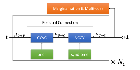
Figure 1: Schematics of the NBP decoder. The main cycle in the gray box is repeated $N_{c}$ times. Inside one cycle there are two phases of computation, the $cv\rightarrow vc$ and $vc\rightarrow cv$ phases which are governed by Eqs. (4) and (5) respectively. The inputs to the neural network are denoted by the green boxes, where the prior and syndrome correspond to $\left\{l_{v}\right\}$ in Eq. (4) and $\left\{s_{c}\right\}$ in Eq. (5) respectively. After each cycle, the set of output $\left\{\mu_{c\to v}\right\}$ is marginalized by Eq. (6) and the resulting $\left\{\mu_{v}\right\}$ is sent to the loss function Eq. (8). We also introduce residual connections to facilitate training of deep networks (He et al., 2015). (See SM for details.)

Neural belief propagation.— The above iterative procedure can be exactly mapped to a deep neural network, where each neuron represents a message $\mu_{c\to v}$ or $\mu_{v\to c}$ (Nachmani et al., 2016). (See Fig. 1.) This permits generalization of the original BP algorithm by introducing additional “trainable” weights $w_{c^{\prime}v,vc}^{\left(t\right)}$ and $w_{cv,v}^{\left(T\right)}$, and “trainable” biases $b_{v}^{\left(t\right)}$ and $b_{v}^{\left(T\right)}$. Specifically, in this NBP algorithm, Eqs. (1, 2, 3) are modified to:

$$\mu_{v\to c}^{\left(t+1\right)}=l_{v}b_{v}^{\left(t\right)}+\sum_{c^{\prime}\in\mathcal{N}\left(v\right)\backslash c}\mu_{c^{\prime}\to v}^{\left(t\right)}w_{c^{\prime}v,vc}^{\left(t\right)},$$ (4)

$$a\left(\mu_{c\to v}^{\left(t+1\right)}\right)=i\pi s_{c}+\sum_{v^{\prime}\in\mathcal{N}\left(c\right)\backslash v}a\left(\mu_{v^{\prime}\to c}^{\left(t\right)}\right),$$ (5)

$$\mu_{v}=l_{v}b_{v}^{\left(T\right)}+\sum_{c\in\mathcal{N}\left(v\right)}\mu_{c\to v}^{\left(T\right)}w_{cv,v}^{\left(T\right)},$$ (6)

respectively (Wymeersch et al., 2011; Nachmani et al., 2016). Notice that all equations above have the form of weighted sum plus bias, interleaved with the nonlinear function $a\left(x\right)=\log\left(\tanh\left(x/2\right)\right)$. This is the canonical form of feed-forward neural networks (Goodfellow et al., 2016). When setting all newly introduced parameters to 1, these equations became the standard BP equations .

To train these weights, one minimizes a carefully designed loss function $\mathcal{L}$ by back-propagating its gradients w.r.t. all trainable parameters. E.g., biases are updated according to $\Delta b_{v}^{(t)}=-lr\times\partial{\mathcal{L}}/\partial{b_{v}^{(t)}}$, where $lr$ is the learning rate. For classical codes, one aims for reproducing the whole error pattern exactly, so the natural choice of the loss function is the binary cross entropy function between the inferred error pattern and the true error pattern:

$$\mathcal{L}\left(\vec{\mu};\mathbf{e}\right)=-\sum_{v}e_{v}\log\sigma\left(\mu_{v}\right)+\left(1-e_{v}\right)\log\left[1-\sigma\left(\mu_{v}\right)\right].$$ (7)

Quantum setting.— Quantum noise can be modeled by random Pauli operators $I$, $\hat{X}$, $\hat{Y}$, and $\hat{Z}$ on the qubits. A convenient way of bookkeeping a $N$-qubit error uses a $2N$-bit string $\mathbf{e}$ representing the Pauli operator: $\hat{\mathcal{P}}\left(\mathbf{e}\right)=\prod_{1\leq i\leq N}\left[\hat{X}_{i}\right]^{e_{i}}\left[\hat{Z}_{i}\right]^{e_{i+N}}$. In this representation, two Pauli-strings operators $\hat{\mathcal{P}}\left(\mathbf{a}\right)$ and $\hat{\mathcal{P}}\left(\mathbf{b}\right)$ commute/anticommute when $\mathbf{a}^{T}M\mathbf{b}$ is even/odd, where the symplectic inner product is defined with $M=\left(\begin{array}[]{cc}&1_{N\times N}\\ 1_{N\times N}\end{array}\right)$. Note that all Pauli-string operators satisfy $\hat{\mathcal{P}}^{2}=1$.

Likewise, the quantum codewords $|\psi\rangle$ are defined by a set of constraints $S_{j}|\psi\rangle=+|\psi\rangle$ where each stabilizer generator $S_{j}$ is a Pauli-string operator. For these equations to have a solution, it is necessary for the $S_{j}$ to mutually commute and to not generate $-1$ under multiplication. Using the above bookkeeping, we can represent each stabilizer generator $S_{j}$ by a $2N$-bit string, and assemble these strings as rows of a parity-check matrix $H$. A quantum LDPC code is one whose parity-check matrix is row- and column-sparse.

There is a crucial difference between classical and quantum error correction. In the classical case, successful decoding means the inferred error $\mathbf{e}^{\mathrm{inf.}}$ is exactly the same as the true error $\mathbf{e}$; while in the quantum case, one only requires the total error $\mathbf{e}^{\mathrm{tot.}}=\mathbf{e}+\mathbf{e}^{\mathrm{inf.}}\mod 2$ to belong to the “stabilizer group” – the set of all Pauli-string operators spanned by the rows of $H$. This is because two Pauli-string operators $E$ and $F=ES_{j}$ that differ by a stabilizer have identical action on all codestates. To test if $\mathbf{e}^{\mathrm{tot.}}$ belongs to the stabilizer group, one simply needs to check that it commutes with all the operators that commute with the stabilizers, i.e., that $H^{\perp}M\mathbf{e}^{\mathrm{tot.}}=\mathbf{0}\mod 2$ where $H^{\perp}$ is the matrix that generates the orthogonal complement of $H$ with respect to the symplectic inner product, $HM\left(H^{\perp}\right)^{T}={\bf 0}\mod 2$.

The above analysis motivates the design the following loss function tailored for quantum error correction:

$$\mathcal{L}\left(\vec{\mu};\mathbf{e}\right)=\sum_{i}f\left(\sum_{jk}H^{\perp}_{ij}M_{jk}\left[e_{k}+\sigma\left(\mu_{k}\right)\right]\right).$$ (8)

Note the parity check $parity\left(x\right)=x\mod 2$ is replaced by the continuous and differentiable function $f\left(x\right)=\left|\sin\left(\pi x/2\right)\right|$ to facilitate gradient-based machine-learning techniques. This loss is minimized when the true error $\mathbf{e}$ and the inferred error $\mathbf{e}^{\mathrm{inf.}}$ sum to a stabilizer.

The loss function can also be averaged over all NBP-cycles $\mathcal{\bar{L}}=\frac{1}{N_{c}}\sum_{i=1}^{N_{c}}\mathcal{L}\left(\vec{\mu}^{\left(i\right)};\mathbf{e}\right),$ which requires marginalization after each cycle. In this work we use a variation of this form. See SM for more details.

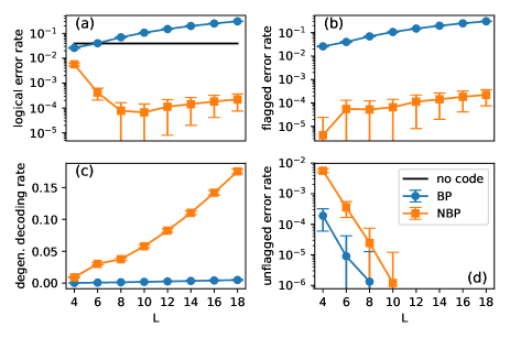
Figure 2: Training the NBP decoder for the toric code with different code sizes. (a) The logical error rate decreases substantially after training (tested at $p_{err}=0.01$). Here the logical error rate is broken up into two terms in (b) and (d), corresponding to “flagged” and “unflagged” errors, respectively. (See main text for details.) (c) The NBP decoder exploits degeneracy by correctly decoding with an error pattern that is not exactly the same as the true error pattern. Training parameters: $N_{c}=25$, $lr=2\times 10^{-4}$.

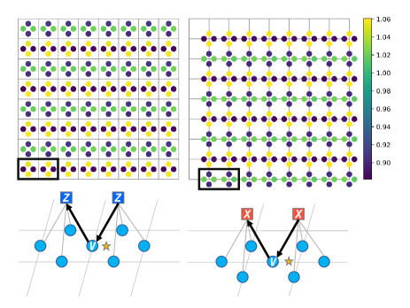
Figure 3: (Top panels) One of the observed patterns of the learned weights for the toric code. To obtain this clear pattern, we implemented weights sharing (see main text) with $\mathbf{G}=\left(2i,2j\right),i,j=0,1,\ldots$ A noisy version of the same pattern is observed when weight sharing is turned off. (Bottom panels) Tanner graph of the toric code and the position of $cvvc$ weights (yellow star). Correspondence to the top panels is marked by the black box.

Toric code.— We first study the toric code (Kitaev, 2006) on an $L\times L$ square lattice, which is a simple and widely studied quantum LDPC. (See Fig. 3 for the local Tanner graph.) During training, we generate error patterns consisting of independent $X$ and $Z$ errors with physical error rate $p_{err}$, i.e., $P\left(e_{v}=1\right)=p_{err}$ for all $v$. In each minibatch, 120 error patterns are drawn from 6 physical error rates that are uniformly distributed in the range $p_{err}\in\left[0.01,0.05\right]$. After $\sim 10000$ minibatches, we test the performance of the trained decoder. Figure 2 compares the original BP decoder (before training) and the trained NBP decoder at $p_{err}=0.01$ for various code sizes. Training significantly enhances decoding accuracy up to three orders of magnitude (Fig. 2a), and we observe that the training time required for convergence depends weakly on the code size $L$. (See SM for details.)

We can distinguish two types of decoding failure. “Flagged” failures occur when the correction inferred by the decoder does not return the system to the code space – there remains a non-trivial syndrome after decoding. “Unflagged” failures occur when the correction return the system to the wrong code state. These two contributions to the overall logical error rate are shown in Fig. 2b and 2d, respectively. We observe that training greatly reduces flagged failures at the expense of slightly increasing unflagged failures, and overall there is a significant net decrease of failures. It should be noted that flagged failures are benign because they can be re-decoded, using either a more accurate but more expensive decoder (e.g. the minimum-weight perfect matching Edmonds (1965)) or a higher layer of code for erasure errors. Such a mixed decoding strategy would combine the speed and flexibility of BP decoder and reliability of a more expensive decoder used on a very small fraction (e.g. $10^{-4}$) of instance.

The loss function Eq. (8) takes into account error degeneracy, and we see on Fig. 2c that the frequency of successful decoding where the actual and the inferred error differ by a stabilizer increases with the code length. This rate was nearly zero with the untrained decoder (see SM for examples of learned stabilizers).

The periodic nature of the toric code inspired us to utilize a weight-sharing technique, where the weights $w_{c_{1}^{\prime}v_{1},v_{1}c_{1}}$ and $w_{c_{2}^{\prime}v_{2},v_{2}c_{2}}$ are invariant under lattice translation $\mathbf{G}$. We can control the amount of sharing by the size of $\mathbf{G}$ (similar to the filter-size in convolutional neural networks). Fig. 3 is a graphical representation of the trained weights, and suggests that symmetry breaking improves BP for quantum codes. We also observe that weights trained on one code size can also increase the performance when applied to codes of different sizes, which implies that the learning is universal/transferable (see SM for more details).

Figure 4 shows that significant improvement can be achieved across a range of physical error rates. Using the original BP, increasing the code size leads to worse performance. After training, performance improves with size for sufficiently low error rates, and the trend indicates that further improved training might lead to a BP decoder with a finite threshold.

When the neural network is initialized away from BP, training gets stuck at a much worse local minimum. This illustrates the importance of incorporating domain knowledge (when possible) before using general machine-learning methods as black boxes, which contrasts with prior uses of neural net decoding of the toric code Torlai and Melko (2017); Krastanov and Jiang (2017).

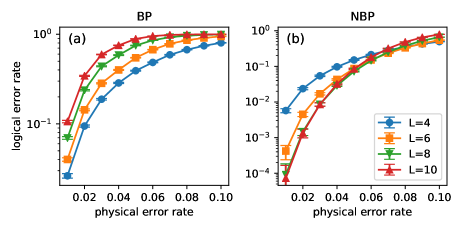
Figure 4: Evolution of the logical error rate as a function of the physical error rate, for the BP/NBP decoder before/after training. (a) Before training the performance of the BP decoder is worse for larger code sizes at all physical error rates. (b) After training, the performance improves substantially for all code sizes at all physical error rates, and the performance curves start to cross each other. This indicates the development of a threshold.

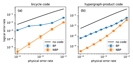
Figure 5: Training greatly improves the BP decoder for quantum LDPC codes with high rates. (a) Quantum bicycle code with code parameter $\left[\left[256,32\right]\right]$ and rate $r=0.125$. Training parameters: $N_{c}=12$, $lr=1\times 10^{-4}$. (b) Quantum hypergraph-product code with code parameter $\left[\left[129,28\right]\right]$ and rate $r\sim 0.2$. Training parameters: $N_{c}=12$, $lr=1\times 10^{-4}$.

Quantum LDPC codes with high rate.— The toric code encodes a constant number $K=2$ of qubits in a growing number $N$ of physical qubits, thus achieving a vanishing rate $r=K/N$. We now turn to quantum LDPC codes with constant rates.

The quantum bicycle code (MacKay et al., 2004) is a quantum LDPC code constructed from a random binary vector $\mathbf{A}$ of size $N/2$. First, all cyclic permutations of $\mathbf{A}$ are collected as columns in a matrix $C$. Then $C$ is concatenated with its transpose to form $H_{0}=\left[C,C^{T}\right]$, from which $K/2$ rows are chosen randomly and removed. After these constructions, $H_{0}$ is a self-dual matrix (meaning $H_{0}H_{0}^{T}=0\mod 2$) of size $\left(N-K\right)/2\times N$. The final parity-check matrix for the quantum bicycle code is $H=\left(\begin{array}[]{cc}H_{0}\\ &H_{0}\end{array}\right)$. The sparsity of this matrix can be controlled by the number of nonzero elements in $\mathbf{A}$. Training the NBP decoder for a quantum bicycle code with $N=256$, $K=32$ and $\sum_{i}A_{i}=8$ improves the accuracy up to 3 orders of magnitude (Fig. 5a).

The quantum hypergraph-product code (Tillich and Zemor, 2014) is constructed from two classical codes with parity-check matrices $\left[H_{1}\right]_{m_{1}\times n_{1}}$ and $\left[H_{2}\right]_{m_{2}\times n_{2}}$. The following products are constructed $H_{X}=\left[\begin{array}[]{cc}H_{1}\otimes I_{n_{2}\times m_{2}},&I_{m_{1}\times n_{1}}\otimes H_{2}^{T}\end{array}\right]$ and $H_{Z}=\left[\begin{array}[]{cc}I_{n_{1}\times m_{1}}\otimes H_{2}&,H_{1}^{T}\otimes I_{m_{2}\times n_{2}}\end{array}\right]$, and the parity-check matrix of the quantum code follows $H=\left(\begin{array}[]{cc}H_{X}\\ &H_{Z}\end{array}\right)$, which performs $m=m_{1}n_{2}+n_{1}m_{2}$ checks on $n=m_{1}m_{2}+n_{1}n_{2}$ qubits. In this paper, we study a hypergraph-product code, for which $H_{1}$ and $H_{2}$ are the classical $\left[7,4,3\right]$ and $\left[15,7,5\right]$ BCH codes, respectively. This code has rate $r=28/129\sim 0.2$. Training the NBP decoder for this code improves the accuracy up to one order of magnitude (Fig. 5b).

Conclusions.— We significantly improved the belief-propagation decoders for quantum LDPC codes by training them as deep neural networks. Our results on the toric code, the quantum bicycle code and the quantum hypergraph-product code all show orders of magnitude of enhancement in decoding accuracy. The original belief propagation is known to have bad performance for quantum error-correcting codes Poulin and Chung (2008). On the other hand, training a neural decoder with general architecture has been reported to be hard for large codes Gruber et al. (2017); Maskara et al. (2018). Our results indicate that combining the general framework of machine learning and the specific domain knowledge of quantum error correction is a promising approach, when neither works well individually.

The significance of this result is supported by the tremendous success of BP with classical LDPC codes (Richardson and Urbanke, 2008), and the fact that quantum LDPC codes promise a low-overhead fault-tolerant quantum computation architecture Gottesman (2014). In addition, our techniques could be adapted to uses of BP in other quantum many-body problems, such as improving the quantum cavity method (Hastings, 2007; Poulin and Bilgin, 2008; Laumann et al., 2008; Poulin and Hastings, 2011).