A priori positivity of solutions to a non-conservative stochastic thin-film equation

Abstract

Stochastic conservation laws are often challenging when it comes to proving existence of non-negative solutions. In a recent work by J. Fischer and G. Grün (2018, Existence of positive solutions to stochastic thin-film equations, SIAM J. Math. Anal.), existence of positive martingale solutions to a conservative stochastic thin-film equation is established in the case of quadratic mobility. In this work, we focus on a larger class of mobilities (including the linear one) for the thin-film model. In order to do so, we need to introduce nonlinear source potentials, thus obtaining a non-conservative version of the thin-film equation. For this model, we assume the existence of a sufficiently regular local solution (i.e., defined up to a stopping time $\tau$) and, by providing suitable conditions on the source potentials and the noise, we prove that such solution can be extended up to any $T>0$ and that it is positive with probability one. A thorough comparison with the aforementioned reference work is provided.

Key words: thin-film equation, drift correction, Itô calculus, nonlinearity, a priori analysis.

AMS (MOS) Subject Classification: 60H15, 35R60, 35G20

1 Introduction

We are interested in stochastic equations driven by random noise in spatial divergence form. A wide class of these equations can be written as

$$\frac{\partial u}{\partial t}=\nabla\cdot\left(m(u)\nabla\frac{\delta F[u]}{\delta u}\right)+\Gamma(u)+\nabla\cdot\left(\sigma\sqrt{m(u)}\mathcal{W}\right)=:\mathscr{D}_{1}+\mathscr{D}_{2}+\mathscr{S},$$ (1)

in the non-negative unknown $u=u(x,t)$, for $x\in D\subset\mathbb{R}^{d}$ and $t>0$. Equation (1) describes the evolution of a system made of a large number of particles. The particles are subject to a gradient-flow dynamics (governed by the free energy $F$ featured in the first drift term $\mathscr{D}_{1}$), to a nonlinear source (given by $\Gamma(u)\equiv\mathscr{D}_{2}$), and to mesoscopic thermal fluctuations (stochastic term $\mathscr{S}$, comprising an infinite-dimensional noise $\mathcal{W}$ and a given scaling parameter $\sigma\neq 0$). The evolution of the system is described by the particle density $u$, which is naturally required to be non-negative. The drift component $\mathscr{D}_{1}$ and the noise term $\mathscr{S}$ satisfy a fluctuation-dissipation relation [2] which can be identified in the powers of the so-called mobility coefficient $m(u)$ being 1 in $\mathscr{D}_{1}$ and $\frac{1}{2}$ in $\mathscr{S}$, respectively.
When $m(u)\equiv u$ and $\Gamma\equiv 0$, equation (1) is known as the Dean-Kawasaki model [6, 10]. This model poses hard mathematical challenges, the first of which is proving existence of positive solutions up to some given time $T>0$. The main difficulties in doing so reside in the nature of the stochastic noise $\mathscr{S}$. To start with, this noise lacks Lipschitz properties and spatial regularity. If, in addition, we assume $\mathcal{W}$ to be a space-time white noise (this is a relevant choice in the physics literature), then the only existence result we are aware of is the recent work [13]. More specifically, in the case of $F(u):=(N/2)\int_{D}{u(x)\log(u(x))\mbox{d}x}$ (corresponding to the Gibbs-Boltzmann entropy functional with pre-factor $N/2>0$), a unique probability measure-valued solution exists if and only if $N\in\mathbb{N}$; however, in this case, the solution is trivial, and coincides with the empirical measure associated with $N$ independent diffusion processes.
Again for $m(u)\equiv u$, and for a specific class of $\Gamma\neq 0$, existence of measure-valued martingale solutions to (1) is available in space dimension one, see the work of von Renesse and coworkers [15, 1, 11, 12]. These results are based on the application of Dirichlet form methods, as well as on the interaction between drift and noise in the context of the Wasserstein geometry over the space of square-integrable probability measures. We also mention [3] for a high-probability existence and uniqueness result for a regularised version of (1).
In this work we investigate a priori positivity of solutions, up to any chosen time $T>0$, in the specific case of a non-conservative thin-film equation

$$\left\{\begin{array}[]{l}\mbox{d}u=-\nabla\cdot\left(m(u)\nabla\left[\Delta u-W^{\prime}(u)\right]\right)\mbox{d}t+\left(h(u)|\nabla u|^{2}+{\color[rgb]{0,0,0}g(u)}\right)\mbox{d}t+\nabla\cdot\left(\sqrt{m(u)}\mbox{d}\mathcal{W}\right),\\ u(x,0)=u_{0}(x)\end{array}\right.$$ (4)

set on the spatial domain $D:=(0,2\pi)$, on some finite time domain $[0,T]$, and on a probability space $(\Omega,\mathcal{F},\mathbb{P})$. More precisely, we assume the existence of a sufficiently regular local solution to (4) (i.e., defined up to a random time $\tau\leq T$) and we show that it can be extended up to $T$ while remaining positive with probability one. Above, $u_{0}\colon D\rightarrow[0,\infty)$ is a suitable positive initial datum, $\mathcal{W}$ is a noise white in time and coloured in space, $m$ is the mobility coefficient, and $W$, $h$ and $g$ are given nonlinear source potentials. These potentials compensate the noise contribution whenever the solution comes close to the singular regimes (these being identified by vanishing or diverging density); this is thoroughly discussed in Sections 3 and 4. The precise nature of $\mathcal{W}$, $W$, $h$, $m$, and ${\color[rgb]{0,0,0}g}$ is stated in Subsection 1.1 below. We highlight that (4) fits into the form prescribed by (1) with $F(u):=\int_{D}{\left\{|\nabla u(x)|^{2}/2+W(u(x))\right\}\mbox{d}x}$ and $\Gamma(u):=h(u)|\nabla u|^{2}+{\color[rgb]{0,0,0}g(u)}$.
Existence of positive martingale solutions to (4) has been established in the conservative case (${\color[rgb]{0,0,0}g}\equiv h\equiv 0$) in [7], for the case of quadratic mobility $m(u)=u^{2}$; this mobility results in a linear multiplicative stochastic noise. The case of general polynomial mobility, including the linear case $m(u)=u$ (corresponding to the noise $\mathscr{S}$ featured in the Dean-Kawasaki model), seems hard to study for the conservative thin-film equation, see [7] again. This is why we analyse (4) for a non-trivial drift component $\Gamma$. However, our drift component $\Gamma$ is not justified, as in the case of [15, 1, 11, 12], by the aforementioned Wasserstein geometry setting. Instead, it is needed in order to deal with algebraic cancellations arising from the Itô calculus applied to relevant functionals of the solution, these functionals being primarily associated with positivity of the solution, which is our main interest here. We also stress the fact that we only pursue a purely analytical justification of our drift component $\Gamma$, and we consequently neglect any physical modelling at this stage.

The paper is organised as follows. Subsection 1.1 contains basic assumptions on the functional setting, on the stochastic noise $\mathcal{W}$, as well as a parametrisation of interest for the relevant nonlinear quantities $m,W,h$, and $g$. Section 2 contains the two main results of this paper, Proposition 2.1 and Theorem 2.2. More specifically, Theorem 2.2 (which is also proved in this section) is concerned with positivity of solutions to (4) up to time $T$, which is our main interest. Its proof builds upon Proposition 2.1, a technical result whose lengthy proof is the topic of Section 3. Sections 4 compares the contents of this paper with the setting and conclusions of [7]. Section 5 illustrates the difficulties that one encounters when trying to prove existence of local solutions to (4) via an approximating Galerkin scheme in the case of general mobility $m$, and also explains why such a scheme is effective in the specific case of quadratic mobility [7]. We summarise our findings and conclusions in Section 6.

1.1 Setting and notation

We work in a periodic function setting on $D:=(0,2\pi)$. The noise $\mathcal{W}$ is white in time and coloured in space. Its covariance operator $Q$ is diagonalisable on the eigenfunctions of the Laplace operator on $D$ with periodic boundary conditions. These eigenfunctions are given by the trigonometric family

$$\left\{e_{r}\right\}_{r=0}^{\infty}:=\left\{\frac{1}{\sqrt{2\pi}},\frac{\sin(x)}{\sqrt{\pi}},\frac{\cos(x)}{\sqrt{\pi}},\frac{\sin(2x)}{\sqrt{\pi}},\frac{\cos(2x)}{\sqrt{\pi}},\frac{\sin(3x)}{\sqrt{\pi}},\frac{\cos(3x)}{\sqrt{\pi}},\cdots\right\}.$$

Using [14, Proposition 2.1.10], we write the noise as $\mathcal{W}(t,x,\omega)=\sum_{r=0}^{\infty}{\sqrt{\lambda_{r}}e_{r}(x)\beta_{r}(t,\omega)}$, where $\{\lambda_{r}\}_{r=0}^{\infty}$ are the eigenvalues of $Q$ associated with $\{e_{r}\}_{r=0}^{\infty}$, and $\{\beta_{r}\}_{r=0}^{\infty}$ is a family of independent Brownian motions. We assume the eigenvalues of $Q$ to be rapidly decaying, say $\lambda_{r}\leq a_{1}e^{-a_{2}r}$, where $a_{1},a_{2}>0$, for all $r\in\mathbb{N}_{0}$.
For some $\epsilon\in(0,1)$, let $A_{0}:=(0,1-\epsilon)$, $A_{1}:=[1-\epsilon,1+\epsilon]$, $A_{\infty}:=(1+\epsilon,\infty)$. The mobility $m$ and the functions $h$ and ${\color[rgb]{0,0,0}g}$ are given by

$$m(u):=\left\{\begin{array}[]{ll}\!u^{\gamma_{1}},&\mbox{ if }u\in A_{0},\\ \!f_{m}(u),&\mbox{ if }u\in A_{1},\\ \!u^{\gamma_{2}},&\mbox{ if }u\in A_{\infty},\end{array}\right.\,\,h(u):=\left\{\begin{array}[]{ll}\!B_{h}u^{-p_{h}},&\mbox{ if }u\in A_{0},\\ \!f_{h}(u),&\mbox{ if }u\in A_{1},\\ \!-B_{h}u^{c_{h}},&\mbox{ if }u\in A_{\infty},\\ \end{array}\right.\,\,g(u):=\left\{\begin{array}[]{ll}\!B_{g}u^{-p_{g}},&\mbox{ if }u\in A_{0},\\ \!f_{g}(u),&\mbox{ if }u\in A_{1},\\ \!-B_{g}u^{c_{g}},&\mbox{ if }u\in A_{\infty},\end{array}\right.$$ (14)

while $W$ is given by $W(u)=u^{-p}$. The functions $m,h,g,$ and $W$ are understood to be infinite when $u\leq 0$. In the above, $p,B_{h},p_{h},c_{h},{\color[rgb]{0,0,0}B_{g},p_{g},c_{g}},\gamma_{1}$, and $\gamma_{2}$ are positive constants, while the functions $f_{h},f_{g}$, and $f_{m}$ are such that $W,h,{\color[rgb]{0,0,0}g}$, and $m$ belong to $\mathcal{C}^{\infty}(0,\infty)$. It is easy to choose $f_{h}$ and $f_{m}$ such that, for some $\delta>0$

$$\,\,f_{m}(u)>\delta, \quad\mbox{for all }u\in A_{1},$$ (15a)

$$\,\,f_{h}^{\prime}(u)\leq-\delta B_{h}, \quad\mbox{for all }u\in A_{1}.$$ (15b)

The potentials $W$, $h$, and the mobility $m$ are sketched in Figure 1, while the potential $g$ is not sketched (as it is qualitatively identical to $h$). We defined $h,{\color[rgb]{0,0,0}g}$ and $m$ piecewise on $A_{0}$ and $A_{\infty}$ in order to be able to treat low and large density regimes differently. The definitions on $A_{1}$ provide smoothness on $(0,\infty)$ for the quantities in (14). Our definitions of $W$, $h$, $g$, and $m$ are justified as follows: the potential $W$ pushes mass away from the repulsive singularity $0$, while obeying the conservation of mass. The source potentials $h$ and ${\color[rgb]{0,0,0}g}$ introduce mass in the system whenever the density is too low, and remove mass whenever the density is too large. In the case of $h$, the rate at which the introduction/removal of mass occurs is proportional to $|\nabla u|^{2}$. The mobility accounts for different drift and noise magnitudes in the low and large density regimes.

    

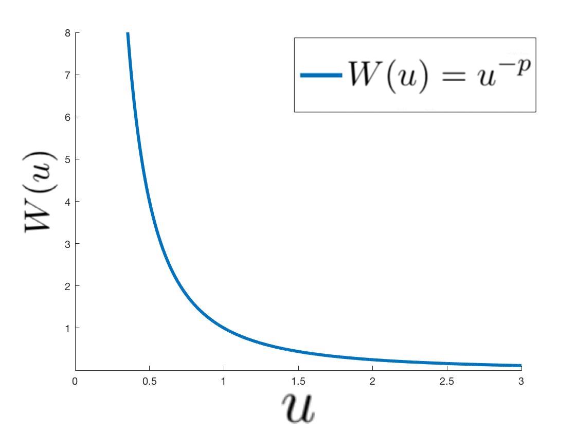
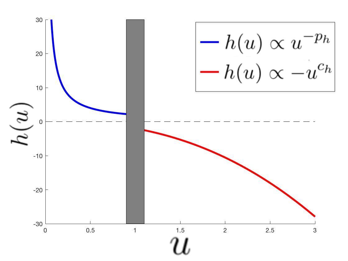
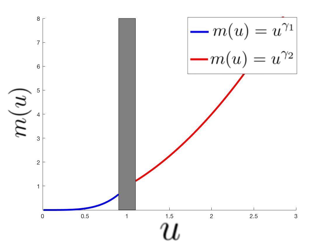
Figure 1: Sketches of $W$ (left), $h$ (centre), and $m$ (right). Plots on $A_{1}$ are not provided for $h$ and $m$. The qualitative behaviour of $g$ is identical to that of $h$.

We use the symbol $L^{p}$ to denote the space $L^{p}(D)$. We use the symbol $W^{s,p}$ to denote the Sobolev space $W_{\mbox{\scriptsize{per}}}^{s,p}(D)$ of $2\pi$-periodic functions on $\mathbb{R}$ having distributional derivates up to order $s$ belonging to $L^{p}$. We abbreviate $H^{s}:=W^{s,2}$. For a Hilbert space $V$, we use $\left\langle\cdot,\cdot\right\rangle_{V}$ and $\|\cdot\|_{V}$ to denote the $V$-inner product and $V$-norm, respectively. We drop the subscript if $V=L^{2}$. For a function $u$ depending on space and time, we often write $u(t)$ instead of $u(x,t)$, and we indifferently use the notations $u_{x}$ and $\nabla u$ to refer to spatial differentiation. Finally, $C$ denotes a generic constant whose value may change from line to line; the dependency of this constant on specific parameters is highlighted whenever relevant.

2 A priori positivity of solutions

Let $T>0$. We show that, if we assume the existence of a sufficiently regular solution to (4) up to a random time $\tau\leq T$, this solution can be extended up to $T$ and is positive $\mathbb{P}$-a.s. In order to do so, we need the following auxiliary result.

Proposition 2.1.

Fix $T>0$ and $\beta>2$. Consider an initial datum $u_{0}\in H^{1}$ such that $\delta_{1}<\min_{x\in D}{u_{0}(x)}$ and $\|u_{0}\|_{H^{1}}<\delta_{2}$, for some $\delta_{2}>\delta_{1}>0$, $\mathbb{P}$-a.s. Assume the existence of a strong solution $u$ to (4) up to a random time $\tau\leq T$. More precisely, we assume the equation below to be satisfied $\mathbb{P}$-a.s., for all $t>0$

$$u(t\wedge\tau) =u_{0}+\int_{0}^{t\wedge\tau}{\left[-\nabla\cdot\left(m(u)\nabla\left[\Delta u-W^{\prime}(u)\right]\right)+\left(h(u)|\nabla u|^{2}+{\color[rgb]{0,0,0}g(u)}\right)\right]\emph{\mbox{d}}s}$$

$$\quad+\int_{0}^{t\wedge\tau}{\nabla\cdot\left(\sqrt{m(u)}(\cdot)\right)\emph{\mbox{d}}\mathcal{W}}.$$ (16)

We assume that $u$ has $\mathbb{P}$-a.s. continuous paths with respect to the $H^{1}$-norm, and that

$$\mathbb{P}\left(\int_{0}^{\tau}{\!\|\nabla u(s)\|^{4}_{L^{4}}\emph{\mbox{d}}s}<\infty\right)=1,\quad\!\mathbb{P}\left(\int_{0}^{\tau}{\!\|\Delta u(s)\|^{2}\emph{\mbox{d}}s}<\infty\right)=1,\quad\!\mathbb{E}\left[\mathchoice{\raisebox{0.0pt}{$\displaystyle{\vphantom{\bigm{|}}\mathopen{}\int_{0}^{\tau}{\!\left\|u_{xxx}(s)\sqrt{m(u(s))}\right\|^{2}\!\emph{\mbox{d}}s}}$}}{\int_{0}^{\tau}{\!\left\|u_{xxx}(s)\sqrt{m(u(s))}\right\|^{2}\!\emph{\mbox{d}}s}}{\int_{0}^{\tau}{\!\left\|u_{xxx}(s)\sqrt{m(u(s))}\right\|^{2}\!\emph{\mbox{d}}s}}{\int_{0}^{\tau}{\!\left\|u_{xxx}(s)\sqrt{m(u(s))}\right\|^{2}\!\emph{\mbox{d}}s}}\right]<\infty.$$ (17)

For all $n\in\mathbb{N}$ such that $n^{-1}<\delta_{1}$ and $n>\delta_{2}$, we assume $\tau_{n}\leq\tau\leq T$, where the stopping time $\tau_{n}$ is given by

$$\tau_{n}:=\inf\left\{t>0:\min_{x\in D}{u(x,t)}\leq n^{-1}\right\}\wedge\inf\left\{t>0:\|u(t)\|_{H^{1}}\geq n\right\}\wedge T.$$ (18)

Assume the following conditions

$$\sum_{r=0}^{\infty}{\lambda_{r}}\mbox{ \emph{is small enough}},$$ (C1)

$$p_{h},B_{h},c_{h}\mbox{ \emph{are big enough}},$$ (C2)

$${\color[rgb]{0,0,0}p_{g},B_{g},c_{g}\mbox{ \emph{are big enough}}}.$$ (C3)

Let $F_{1}\colon H^{1}\rightarrow\mathbb{R}\cup\{\infty\}\colon u\mapsto\int_{D}{|u|^{-\beta}}$, let $F_{2}\colon H^{1}\rightarrow\mathbb{R}\colon u\mapsto\frac{1}{2}\|u\|^{2}_{H^{1}}$, and let $F:=F_{1}+F_{2}$. There is a constant $C$ independent of $n$, such that

$$\mathbb{E}\left[\mathchoice{\raisebox{0.0pt}{$\displaystyle{\vphantom{\bigm{|}}\mathopen{}F(u(t\wedge\tau_{n}))}$}}{F(u(t\wedge\tau_{n}))}{F(u(t\wedge\tau_{n}))}{F(u(t\wedge\tau_{n}))}\right]\leq C,\qquad\mbox{for all }t\in[0,T].$$ (19)

The proof of Proposition 2.1, which is quite lengthy and technical, is the content of Section 3. Our main result, which relies on Proposition 2.1, is the following.

Theorem 2.2.

Let the assumptions of Proposition 2.1 be satisfied. Then the solution $u$ to (2.1) is defined up to time $T$ and is $\mathbb{P}$-a.s. positive, meaning that

$$\mathbb{P}\left(u(x,t)>0\mbox{ for all }x\mbox{ in }D\mbox{ and for all }t\in[0,T]\right)=1.$$

Proof.

Define $\theta:=\frac{\beta}{2}-1>0$. The Hölder inequality and the bound $u^{-\theta}\leq u^{-\beta}+1$, valid on $(0,\infty)$, give

$$\|u^{-\theta}(t\wedge\tau_{n})\|_{W^{1,1}} =\int_{D}{|u^{-\theta}(t\wedge\tau_{n})|\mbox{d}x}+\theta\int_{D}{|u^{-\theta-1}(t\wedge\tau_{n})\nabla u(t\wedge\tau_{n})|\mbox{d}x}$$

$$\leq\int_{D}{|u^{-\theta}(t\wedge\tau_{n})|\mbox{d}x}+\theta\left(\int_{D}{|u^{-2(\theta+1)}(t\wedge\tau_{n})|\mbox{d}x}\right)^{1/2}\left(\int_{D}{|\nabla u(t\wedge\tau_{n})|^{2}\mbox{d}x}\right)^{1/2}$$

$$\leq C+C\int_{D}{|u^{-\beta}(t\wedge\tau_{n})|\mbox{d}x}+C\|u(t\wedge\tau_{n})\|^{2}_{H^{1}}\leq C+CF(u(t\wedge\tau_{n})).$$

This immediately entails, using Proposition 2.1, that

$$\mathbb{E}\left[\mathchoice{\raisebox{0.0pt}{$\displaystyle{\vphantom{\bigm{|}}\mathopen{}\|u^{-\theta}(t\wedge\tau_{n})\|_{W^{1,1}}}$}}{\|u^{-\theta}(t\wedge\tau_{n})\|_{W^{1,1}}}{\|u^{-\theta}(t\wedge\tau_{n})\|_{W^{1,1}}}{\|u^{-\theta}(t\wedge\tau_{n})\|_{W^{1,1}}}\right]\leq C,\qquad\mbox{for all }t\in[0,T],$$ (20)

where $C$ is independent of $n$. Let $t\in[0,T]$. We use the $\mathbb{P}$-a.s. $H^{1}$-continuity of the paths of $u$, the continuous embedding $W^{1,1}\hookrightarrow C(0,2\pi)$ (with embedding constant $K_{1}$), the Chebyshev inequality, and equations (19) and (20) to deduce

$$\mathbb{P}\left(\tau_{n}<t\right) \leq\mathbb{P}\left(\min_{x\in D}{|u(t\wedge\tau_{n})|}\leq n^{-1}\right)+\mathbb{P}\left(\|u(t\wedge\tau_{n})\|_{H^{1}}\geq n\right)=\mathbb{P}\left(\max_{x\in D}{|u(t\wedge\tau_{n})|^{-\theta}}\geq n^{\theta}\right)$$

$$\quad+\mathbb{P}\left(\|u(t\wedge\tau_{n})\|^{2}_{H^{1}}\geq n^{2}\right)\leq\mathbb{P}\left(\|u^{-\theta}(t\wedge\tau_{n})\|_{W^{1,1}}\geq K_{1}^{-1}n^{\theta}\right)+\mathbb{P}\left(\|u(t\wedge\tau_{n})\|^{2}_{H^{1}}\geq n^{2}\right)$$

$$\leq\frac{\mathbb{E}\left[\mathchoice{\raisebox{0.0pt}{$\displaystyle{\vphantom{\bigm{|}}\mathopen{}\|u^{-\theta}(t\wedge\tau_{n})\|_{W^{1,1}}}$}}{\|u^{-\theta}(t\wedge\tau_{n})\|_{W^{1,1}}}{\|u^{-\theta}(t\wedge\tau_{n})\|_{W^{1,1}}}{\|u^{-\theta}(t\wedge\tau_{n})\|_{W^{1,1}}}\right]}{K_{1}^{-1}n^{\theta}}+\frac{\mathbb{E}\left[\mathchoice{\raisebox{0.0pt}{$\displaystyle{\vphantom{\bigm{|}}\mathopen{}\|u(t\wedge\tau_{n})\|^{2}_{H^{1}}}$}}{\|u(t\wedge\tau_{n})\|^{2}_{H^{1}}}{\|u(t\wedge\tau_{n})\|^{2}_{H^{1}}}{\|u(t\wedge\tau_{n})\|^{2}_{H^{1}}}\right]}{n^{2}}\rightarrow 0$$

as $n\rightarrow 0$. This implies that $\mathbb{P}\left(\sup_{n}{\tau_{n}}=T\right)=1$, and concludes the proof. ∎

3 Proof of Proposition 2.1

We split the proof in four parts. In Subsection 3.1, we compute and properly bound the Itô differential of the process $F(u)$ up to time $t\wedge\tau_{n}$, for any $t\in[0,T]$. In Subsection 3.2, we group all the terms from the previously computed Itô differential into families, each family being characterised by a specific term. Subsections 3.3 and 3.4 are concerned with imposing conditions on the parameters $p,B_{h},p_{h},c_{h},{\color[rgb]{0,0,0}B_{g},p_{g},c_{g}},\gamma_{1},\gamma_{2}$, and $\{\lambda_{r}\}_{r=0}^{\infty}$ in such a way that (19) is achieved; more specifically, Subsection 3.3 provides the relevant analysis on $A_{0}\cup A_{\infty}$, while Subsection 3.4 consistently extends this analysis on to $A_{1}$.
For notational convenience, we rewrite (2.1) as $\mbox{d}u=\phi(u(t))\mbox{d}t+\Phi(u(t))\mbox{d}\mathcal{W}(t),$ where

$$\phi(u)=\phi_{1}(u)+\phi_{2}(u)+\phi_{3}(u) :=-\nabla\cdot\left(m(u)\nabla\left[\Delta u-W^{\prime}(u)\right]\right)+h(u)|\nabla u|^{2}+{\color[rgb]{0,0,0}g(u)},$$

$$\Phi(u)v :=\nabla\cdot\left(\sqrt{m(u)}v\right).$$

Integration by parts entails that the component of the stochastic noise of (2.1) along the direction $e_{i}$, for $i\in\mathbb{N}_{0}$, is

$$\left\langle\int_{0}^{t}{\Phi(u(s))\mbox{d}\mathcal{W}(s)},e_{i}\right\rangle=\left\langle\int_{0}^{t}{\nabla\cdot\left(\sqrt{m(u(s))}\sum_{r=0}^{\infty}{\sqrt{\lambda_{r}}e_{r}\mbox{d}\beta_{r}(s)}\right)},e_{i}\right\rangle$$

$$=-\left\langle\int_{0}^{t}{\sqrt{m(u(s))}\sum_{r=0}^{\infty}{\sqrt{\lambda_{r}}e_{r}\mbox{d}\beta_{r}(s)}},\nabla e_{i}\right\rangle=\sum_{r=0}^{\infty}{\int_{0}^{t}{-\left\langle\sqrt{m(u(s))}e_{r},\nabla e_{i}\right\rangle\sqrt{\lambda_{r}}\mbox{d}\beta_{r}(s)}}.$$

Thus $\Phi$ can be thought of as an infinite-dimensional noise represented with components given by

$$\Phi_{i,r}(u(s)):=-\left\langle\sqrt{m(u(s))}e_{r},\nabla e_{i}\right\rangle,\qquad\mbox{for all }i,r\in\mathbb{N}_{0}.$$ (21)

3.1 Itô formula for $F(u(t\wedge\tau_{n}))$

We use the Itô formula

$$G(u(t\wedge\tau_{n})) =G(u(0))+\int_{0}^{t\wedge\tau_{n}}{\!G_{u}(u(s))\phi(u(s))\mbox{d}s}+\int_{0}^{t\wedge\tau_{n}}{\frac{1}{2}\mbox{Tr}\!\left[G_{uu}(u(s))(\Phi(u(s))Q^{\frac{1}{2}})(\Phi(u(s))Q^{\frac{1}{2}})^{T}\right]\!\mbox{d}s}$$

$$\quad+\int_{0}^{t\wedge\tau_{n}}{G_{u}(u(s))\Phi(u(s))\mbox{d}\mathcal{W}(s)}+=:I_{1}+I_{2}+I_{3}+I_{4},$$ (22)

here stated for a real-valued functional $G$ applied to the solution $u$. We can apply (3.1) to $G=F_{1}$ and $G=F_{2}$ because, up to time $t\wedge\tau_{n}$, they are both uniformly continuous (along with their first and second derivatives) over bounded sets of $H^{1}$. We analyse terms $I_{2}$, $I_{3}$, and $I_{4}$ of (3.1) for $G=F_{1}$ and $G=F_{2}$. Time dependence is often dropped for notational convenience.
Term $I_{2}$ for $G=F_{1}$. The first and second derivatives of $F_{1}$ are $F_{1,u}(u)v=-\beta\int_{D}{u^{-\beta-1}v\mbox{d}x}$ and $F_{1,uu}(u)(v_{1},v_{2})=\beta(\beta+1)\int_{D}{u^{-\beta-2}v_{1}v_{2}\mbox{d}x}$. We study the contributions of $\phi_{1}$, $\phi_{2}$, and $\phi_{3}$ on $F_{1,u}(u)\phi(u)$ separately. We obtain

$$F_{1,u}(u)\phi_{1}(u) =\left\langle-\nabla\cdot\left(m(u)\nabla\left[\Delta u-W^{\prime}(u)\right]\right),-\beta u^{-\beta-1}\right\rangle=\beta(\beta+1)\left\langle m(u)\nabla[\Delta u-W^{\prime}(u)],u^{-\beta-2}\nabla u\right\rangle$$

$$=\beta(\beta+1)\left\langle\nabla[\Delta u-W^{\prime}(u)],m(u)u^{-\beta-2}\nabla u\right\rangle=-\beta(\beta+1)\left\langle\Delta u,\nabla(m(u)u^{-\beta-2}\nabla u)\right\rangle+$$

$$\quad\quad-\beta(\beta+1)\left\langle W^{\prime\prime}(u)\nabla u,m(u)u^{-\beta-2}\nabla u\right\rangle$$

$$=-\beta(\beta+1)\left\langle\Delta u,m(u)u^{-\beta-2}\Delta u\right\rangle-\beta(\beta+1)\left\langle\Delta u,(m(u)u^{-\beta-2})^{\prime}|\nabla u|^{2}\right\rangle$$

$$\quad\quad-\beta(\beta+1)\left\langle W^{\prime\prime}(u)\nabla u,m(u)u^{-\beta-2}\nabla u\right\rangle.$$

We remind the reader of the identity

$$\left\langle f(u)|\nabla u|^{2},\Delta u\right\rangle=-\frac{1}{3}\left\langle f^{\prime}(u)|\nabla u|^{2},|\nabla u|^{2}\right\rangle,$$ (23)

which is valid for $f\in\mathcal{C}^{1}(0,\infty)$. We choose $f(u):=(m(u)u^{-\beta-2})^{\prime}$ and deduce

$$F_{1,u}(u)\phi_{1}(u) =-\beta(\beta+1)\left\langle\Delta u,m(u)u^{-\beta-2}\Delta u\right\rangle$$

$$\quad+\frac{\beta(\beta+1)}{3}\left\langle(m(u)u^{-\beta-2})^{\prime\prime}|\nabla u|^{2},|\nabla u|^{2}\right\rangle-\beta(\beta+1)\left\langle W^{\prime\prime}(u)\nabla u,m(u)u^{-\beta-2}\nabla u\right\rangle.$$ (24)

As for $\phi_{2}$ and $\phi_{3}$, the contributions are simply

$$F_{1,u}(u)\phi_{2}(u)=\left\langle h(u)|\nabla u|^{2},-\beta u^{-\beta-1}\right\rangle,\qquad{\color[rgb]{0,0,0}F_{1,u}(u)\phi_{3}(u)}={\color[rgb]{0,0,0}\left\langle g(u),-\beta u^{-\beta-1}\right\rangle.}$$ (25)

Term $I_{2}$ for $G=F_{2}$. The first and second derivatives of $F_{2}$ are $F_{2,u}(u)v=\left\langle u,v\right\rangle_{H^{1}}$ and $F_{2,uu}(u)(v_{1},v_{2})=\left\langle v_{1},v_{2}\right\rangle_{H^{1}}$. We study the contributions of $\phi_{1}$, $\phi_{2}$, and $\phi_{3}$ on $F_{2,u}(u)\phi(u)$ separately. We set $f(u):=m(u)W^{\prime\prime}(u)$ and we obtain, by relying on (23) and using integration by parts

$$F_{2,u}(u)\phi_{1}(u)$$

$$\quad=\left\langle-\nabla\cdot\left(m(u)\nabla\left[\Delta u-W^{\prime}(u)\right]\right),u\right\rangle_{H^{1}}=\left\langle-\nabla\cdot\left(m(u)\nabla\left[\Delta u-W^{\prime}(u)\right]\right),u\right\rangle$$

$$\quad\quad+\left\langle\nabla(-\nabla\cdot\left(m(u)\nabla\left[\Delta u-W^{\prime}(u)\right]\right)),\nabla u\right\rangle$$

$$\quad=\left\langle m(u)\nabla[\Delta u-W^{\prime}(u)],\nabla u\right\rangle+\left\langle\nabla\cdot(m(u)\nabla[\Delta u-W^{\prime}(u)]),\Delta u\right\rangle$$

$$\quad=\left\langle\nabla[\Delta u-W^{\prime}(u)],m(u)\nabla u\right\rangle-\left\langle m(u)\nabla[\Delta u-W^{\prime}(u)],u_{xxx}\right\rangle$$

$$\quad=-\left\langle\Delta u,m^{\prime}(u)|\nabla u|^{2}\right\rangle-\left\langle\Delta u,m(u)\Delta u\right\rangle-\left\langle W^{\prime\prime}(u)\nabla u,m(u)\nabla u\right\rangle-\left\langle m(u)u_{xxx},u_{xxx}\right\rangle+\left\langle f(u)\nabla u,u_{xxx}\right\rangle$$

$$\quad=\frac{1}{3}\left\langle m^{\prime\prime}(u)|\nabla u|^{2},|\nabla u|^{2}\right\rangle-\left\langle\Delta u,m(u)\Delta u\right\rangle-\left\langle W^{\prime\prime}(u)\nabla u,m(u)\nabla u\right\rangle$$

$$\quad\quad-\left\langle m(u)u_{xxx},u_{xxx}\right\rangle-\left\langle f(u)\Delta u,\Delta u\right\rangle-\left\langle f^{\prime}(u)|\nabla u|^{2},\Delta u\right\rangle$$

$$\quad=\frac{1}{3}\left\langle\left[m^{\prime\prime}(u)+f^{\prime\prime}(u)\right]|\nabla u|^{2},|\nabla u|^{2}\right\rangle-\left\langle\Delta u,m(u)[1+W^{\prime\prime}(u)]\Delta u\right\rangle$$

$$\quad\quad-\left\langle W^{\prime\prime}(u)\nabla u,m(u)\nabla u\right\rangle-\left\langle m(u)u_{xxx},u_{xxx}\right\rangle.$$ (26)

The contribution associated with $\phi_{2}$ is

$$F_{2,u}(u)\phi_{2}(u) =\left\langle h(u)|\nabla u|^{2},u\right\rangle_{H^{1}}=\left\langle h(u)u,|\nabla u|^{2}\right\rangle+\left\langle\nabla(h(u)|\nabla u|^{2}),\nabla u\right\rangle$$

$$=\left\langle h(u)u,|\nabla u|^{2}\right\rangle-\left\langle h(u)|\nabla u|^{2},\Delta u\right\rangle=\left\langle h(u)u,|\nabla u|^{2}\right\rangle+\frac{1}{3}\left\langle h^{\prime}(u)|\nabla u|^{2},|\nabla u|^{2}\right\rangle,$$ (27)

while the contribution associated with $\phi_{3}$ is

$$F_{2,u}(u)\phi_{3}(u) =\left\langle g(u),u\right\rangle+\left\langle g^{\prime}(u)\nabla u,\nabla u\right\rangle.$$ (28)

Term $I_{3}$ for $G=F_{1}$. We rely on (21) and the expression of $F_{1,uu}$ to compute the Itô correction

$$\frac{1}{2}\mbox{Tr}\left[F_{1,uu}(u)(\Phi(u)Q^{1/2})(\Phi(u)Q^{1/2})^{T}\right]$$

$$\quad=\beta(\beta+1)\sum_{r=0}^{\infty}{\lambda_{r}\sum_{s=0}^{\infty}{\sum_{z=0}^{\infty}{\left\langle u^{-\beta-2}e_{z},e_{s}\right\rangle\left\langle\sqrt{m(u)}e_{r},e_{s,x}\right\rangle\left\langle\sqrt{m(u)}e_{r},e_{z,x}\right\rangle}}}.$$ (29)

Remark 3.1.

One can convince oneself of the nature of (3.1) by thinking of a finite-dimensional equivalent of the problem, formulated in terms of the matrices

$$Q_{m}=\mbox{diag}\left\{\sqrt{\lambda_{1}},\cdots,\sqrt{\lambda_{m}}\right\},\quad\left[\Phi_{m}(u)\right]_{i,r}:=-\left\langle\sqrt{m(u)}e_{r},\nabla e_{i}\right\rangle,\quad i,r\in\{0,\cdots,m\},$$ (30)

$$\left[F_{1,uu}(u)\right]_{m}(e_{i},e_{r})=\beta(\beta+1)\int_{D}{u^{-\beta-2}e_{i}e_{r}\mbox{d}x},\quad i,r\in\{0,\cdots,m\}.$$

We bound (3.1) by using integration by parts, the Parseval identity in $L^{2}$ (for the sums over $z$ and $s$), the rapid decay of $\{\lambda_{r}\}_{r=0}^{\infty}$, and the fact that $\|(\mbox{d}^{k}/\mbox{d}x^{k})e_{r}\|_{L^{\infty}}\leq C_{k}r^{k}$ (for the sum over $r$). We obtain

$$\beta(\beta+1)\sum_{r=0}^{\infty}{\lambda_{r}\sum_{s=0}^{\infty}{\sum_{z=0}^{\infty}{\left\langle u^{-\beta-2}e_{z},e_{s}\right\rangle\left\langle\sqrt{m(u)}e_{r},e_{s,x}\right\rangle\left\langle\sqrt{m(u)}e_{r},e_{z,x}\right\rangle}}}$$

$$\quad=\beta(\beta+1)\sum_{r=0}^{\infty}{\lambda_{r}\sum_{s=0}^{\infty}{\sum_{z=0}^{\infty}{\left\langle u^{-\beta-2}e_{z},e_{s}\right\rangle\left\langle\nabla\left(\sqrt{m(u)}e_{r}\right),e_{s}\right\rangle\left\langle\nabla\left(\sqrt{m(u)}e_{r}\right),e_{z}\right\rangle}}}$$

$$\quad=\beta(\beta+1)\sum_{r=0}^{\infty}{\lambda_{r}\sum_{s=0}^{\infty}{\left\langle\nabla\left(\sqrt{m(u)}e_{r}\right),e_{s}\right\rangle\left\langle\nabla\left(\sqrt{m(u)}e_{r}\right),u^{-\beta-2}e_{s}\right\rangle}}$$

$$\quad=\beta(\beta+1)\sum_{r=0}^{\infty}{\lambda_{r}\left\langle\left|\nabla\left(\sqrt{m(u)}e_{r}\right)\right|^{2},u^{-\beta-2}\right\rangle}$$ (31)

$$\quad\leq C(\beta,\{\lambda\}_{r})\left\{\left\langle m^{-1}(u)(m^{\prime}(u))^{2}u^{-\beta-2}\,\nabla u,\nabla u\right\rangle+\int_{D}{m(u)u^{-\beta-2}\mbox{d}x}\right\}.$$ (32)

Remark 3.2.

Alternatively, one can identify (31) by using [4, Section 3].

Term $I_{3}$ for $G=F_{2}$. We compute the Itô correction

$$\frac{1}{2}\mbox{Tr}\left[F_{2,uu}(u)(\Phi(u)Q^{1/2})(\Phi(u)Q^{1/2})^{T}\right]=\sum_{r=0}^{\infty}{\lambda_{r}\sum_{z=0}^{\infty}{(1+z^{2})\left\langle\sqrt{m(u)}e_{r},e_{z,x}\right\rangle^{2}}}$$ (33)

$$\quad=\sum_{r=0}^{\infty}{\lambda_{r}\sum_{z=0}^{\infty}{\left\langle\sqrt{m(u)}e_{r},e_{z,x}\right\rangle^{2}}}+\sum_{r=0}^{\infty}{\lambda_{r}\sum_{z=0}^{\infty}{z^{2}\left\langle\sqrt{m(u)}e_{r},e_{z,x}\right\rangle^{2}}}=:T_{1}+T_{2}.$$

Once again, the reader can convince oneself of the nature of (33) by thinking of a finite-dimensional equivalent of the problem, thus relying on the matrices $Q_{m}$ and $\Phi_{m}(u)$ defined in (30), as well as on the matrix $[F_{2,uu}(u)]_{m}=\mbox{diag}\{(1+z^{2})\}_{z=1,\cdots,m}$. See Remark 3.1 also.

We bound $T_{2}$. Given the nature of the trigonometric basis $\{e_{r}\}_{r=0}^{\infty}$, we have (for $r\geq 1$), that $re_{r,x}=\delta(r)\Delta e_{\sigma(r)}$, for some injective function $\sigma:\mathbb{N}\rightarrow\mathbb{N}$ and where $\delta(r)\in\{-1;+1\}$. We use integration by parts and the Parseval identity (for the sum over $z$) and obtain

$$T_{2} =\sum_{r=0}^{\infty}{\lambda_{r}\sum_{z=0}^{\infty}{\left\langle\sqrt{m(u)}e_{r},\Delta e_{z}\right\rangle^{2}}}=\sum_{r=0}^{\infty}{\lambda_{r}\sum_{z=0}^{\infty}{\left\langle\Delta\left(\sqrt{m(u)}e_{r}\right),e_{z}\right\rangle^{2}}}=\sum_{r=0}^{\infty}{\lambda_{r}\left\|\Delta\left(\sqrt{m(u)}e_{r}\right)\right\|^{2}}$$ (34)

$$\leq C\sum_{r=0}^{\infty}{\lambda_{r}\left[\left\|\left\{-\frac{1}{4}m^{-3/2}(m^{\prime})^{2}+\frac{1}{2}m^{-1/2}(u)m^{\prime\prime}(u)\right\}|\nabla u|^{2}e_{r}\right\|^{2}+\left\|\frac{1}{2}m^{-1/2}(u)m^{\prime}(u)\Delta ue_{r}\right\|^{2}\right.}$$ (35)

$$\quad+\left.\left\|m^{-1/2}(u)m^{\prime}(u)\nabla u\,e_{r,x}\right\|^{2}+\left\|\sqrt{m(u)}\Delta e_{r}\right\|^{2}\right]$$

$$\leq C(\{\lambda_{r}\}_{r})\left\{\left\langle\left[m^{-1}(u)(m^{\prime\prime}(u))^{2}+m^{-3}(u)(m^{\prime}(u))^{4}\right]\nabla u|^{2},|\nabla u|^{2}\right\rangle\right.$$

$$\quad+\left.\left\langle m^{-1}(u)(m^{\prime}(u))^{2}\Delta u,\Delta u\right\rangle+\left\langle m^{-1}(u)(m^{\prime}(u))^{2}\nabla u,\nabla u\right\rangle+\int_{D}{m(u)\mbox{d}x}\right\},$$ (36)

where the right-hand-side of (34) can also be inferred from [4, Section 3].

Remark 3.3.

Given the polynomial nature of $m(u)\left|{}_{A_{0}\cup A_{\infty}}\right.$, it is easy to notice that the multiplying term $T_{3}:=-\frac{1}{4}m^{-3/2}(m^{\prime})^{2}+\frac{1}{2}m^{-1/2}(u)m^{\prime\prime}(u)$ in (35) vanishes if and only if $\gamma_{1}=\gamma_{2}=2$. In all other cases, the terms making up $T_{3}$ are proportional to each other.

As for $T_{1}$, the computation is simpler, and it reads, thanks to the Parseval inequality

$$T_{1} =\sum_{r=0}^{\infty}{\lambda_{r}\sum_{z=0}^{\infty}{\left\langle\sqrt{m(u)}e_{r},e_{z,x}\right\rangle^{2}}}=\sum_{r=0}^{\infty}{\lambda_{r}\sum_{z=0}^{\infty}{\left\langle\nabla\left(\sqrt{m(u)}e_{r}\right),e_{z}\right\rangle^{2}}}=\sum_{r=0}^{\infty}{\lambda_{r}\left\|\nabla\left(\sqrt{m(u)}e_{r}\right)\right\|^{2}}$$ (37)

$$\leq C\sum_{r=0}^{\infty}{\lambda_{r}\!\left[\left\|m^{-1/2}(u)m^{\prime}(u)\nabla u\,e_{r}\right\|^{2}+\left\|\sqrt{m(u)}e_{r,x}\right\|^{2}\right]}$$ (38)

$$\leq C(\{\lambda_{r}\}_{r})\left\{\left\langle m^{-1}(u)(m^{\prime}(u))^{2}\nabla u,\nabla u\right\rangle+\int_{D}{m(u)\mbox{d}x}\right\},$$

where the right-hand-side of (37) can once again be inferred from [4, Section 3]. We deduce

$$\frac{1}{2}\mbox{Tr}\left[F_{2,uu}(u)(\Phi(u)Q^{1/2})(\Phi(u)Q^{1/2})^{T}\right]\leq C(\{\lambda_{r}\}_{r})\left\{\left\langle\left[m^{-1}(u)(m^{\prime\prime}(u))^{2}+m^{-3}(u)(m^{\prime}(u))^{4}\right]|\nabla u|^{2},|\nabla u|^{2}\right\rangle\right.$$

$$\quad\quad+\left.\left\langle m^{-1}(u)(m^{\prime}(u))^{2}\Delta u,\Delta u\right\rangle+\left\langle m^{-1}(u)(m^{\prime}(u))^{2}\nabla u,\nabla u\right\rangle+\int_{D}{m(u)\mbox{d}x}\right\},$$ (39)

Term $I_{4}$ for $G=F_{1}$. We rely on [5, Theorem 4.36] and bound the Itô isometry term associated with $I_{4}$. We use integration by parts and the Parseval identity to deduce

$$\sum_{r=0}^{\infty}{\lambda_{r}\left|\sum_{z=0}^{\infty}{-\beta\left\langle u^{-\beta-1},e_{z}\right\rangle\left\langle\nabla\left(\sqrt{m(u)}e_{r}\right),e_{z}\right\rangle}\right|^{2}}=\beta\sum_{r=0}^{\infty}{\lambda_{r}\left|\left\langle u^{-\beta-1},\nabla\left(\sqrt{m(u)}e_{r}\right)\right\rangle\right|^{2}}$$

$$\quad=\beta\sum_{r=0}^{\infty}{\lambda_{r}\left|\left\langle(\beta+1)u^{-\beta-2}\nabla u,\sqrt{m(u)}e_{r}\right\rangle\right|^{2}}\leq C(\{\lambda_{r}\}_{r},\beta)\left\langle u^{-\beta-2}m(u)\nabla u,u^{-\beta-2}\nabla u\right\rangle.$$ (40)

Given the definition of $\tau_{n}$, we deduce that $I_{4}$ is a square-integrable martingale with mean zero, see [5, Proposition 4.28]. The contribution of $I_{4}$ can thus be neglected.

Term $I_{4}$ for $G=F_{2}$. Again relying on [5, Theorem 4.36], we bound the Itô isometry term associated with $I_{2}$. Similarly to (3.1), we deduce

$$\sum_{r=0}^{\infty}{\lambda_{r}\left|\sum_{z=0}^{\infty}{(1+z^{2})\left\langle u,e_{z}\right\rangle\left\langle\nabla\left(\sqrt{m(u)}e_{r}\right),e_{z}\right\rangle}\right|^{2}}=\sum_{r=0}^{\infty}{\lambda_{r}\left|\sum_{z=0}^{\infty}{\left\langle u,e_{z}-\Delta e_{z}\right\rangle\left\langle\nabla\left(\sqrt{m(u)}e_{r}\right),e_{z}\right\rangle}\right|^{2}}$$

$$\quad\leq\sum_{r=0}^{\infty}{2\lambda_{r}\left|\left\langle u,\nabla\left(\sqrt{m(u)}e_{r}\right)\right\rangle\right|^{2}}+\sum_{r=0}^{\infty}{2\lambda_{r}\left|\left\langle\Delta u,\nabla\left(\sqrt{m(u)}e_{r}\right)\right\rangle\right|^{2}}$$

$$\quad=\sum_{r=0}^{\infty}{2\lambda_{r}\left|\left\langle\nabla u,\sqrt{m(u)}e_{r}\right\rangle\right|^{2}}+\sum_{r=0}^{\infty}{2\lambda_{r}\left|\left\langle u_{xxx},\sqrt{m(u)}e_{r}\right\rangle\right|^{2}}$$

$$\quad\leq C(\{\lambda_{r}\}_{r})\left\{\left\langle\nabla u,m(u)\nabla u\right\rangle+\left\langle u_{xxx},m(u)u_{xxx}\right\rangle\right\}.$$ (41)

In this case, the definition of $\tau_{n}$ does not imply that $I_{4}$ is a square-integrable martingale with mean zero. This is due to the presence of the term $\left\langle u_{xxx},m(u)u_{xxx}\right\rangle$.

3.2 Clustering contributions from the Itô formula

In the previous section we have provided bounds for the terms $I_{2}$, $I_{3}$, $I_{4}$ associated with the Itô formula applied to the functionals $F_{1}(u)$ and $F_{2}(u)$. These bounds contain terms which can be clustered in five distinct families, identified as

$$\int_{D}{p(u)},$$ (F1)

$$\left\langle p(u)\Delta u,\Delta u\right\rangle,$$ (F2)

$$\left\langle p(u)|\nabla u|^{2},|\nabla u|^{2}\right\rangle,$$ (F3)

$$\left\langle p(u)\nabla u,\nabla u\right\rangle,$$ (F4)

$$\left\langle p(u)u_{xxx},u_{xxx}\right\rangle,$$ (F5)

for some $p\in\mathcal{C}(0,\infty)$. Notice that all contributions to the Itô formula are well defined, because of assumption (17). With the exception of the terms in the right-hand-side of (3.1) (associated with the Itô isometry of $I_{4}$ for the functional $F_{1}(u)$), we now cluster all the terms belonging to the same family.
Terms of kind (F1). Relevant terms are gathered from (3.1), (32), (28), (25), adding up to

$$C(\{\lambda_{r}\}_{r})\int_{D}{m(u)\mbox{d}x}+C(\{\lambda_{r}\}_{r},\beta)\int_{D}{m(u)u^{-\beta-2}\mbox{d}x}{\color[rgb]{0,0,0}+\left\langle g(u),u\right\rangle+\left\langle g(u),-\beta u^{-\beta-1}\right\rangle}.$$ (42)

Terms of kind (F2). Relevant terms are gathered from (3.1), (3.1), (3.1), adding up to

$$-\beta(\beta+1)\left\langle\Delta u,m(u)u^{-\beta-2}\Delta u\right\rangle-\left\langle\Delta u,m(u)\Delta u\right\rangle-\left\langle\Delta u,m(u)W^{\prime\prime}(u)\Delta u\right\rangle$$

$$\quad+C(\{\lambda_{r}\}_{r})\left\langle m^{-1}(u)(m^{\prime}(u))^{2}\Delta u,\Delta u\right\rangle.$$ (43)

Terms of kind (F3). Relevant terms are gathered from (3.1), (3.1), (3.1), (3.1), adding up to

$$C(\beta)\left\langle(m(u)u^{-\beta-2})^{\prime\prime}|\nabla u|^{2},|\nabla u|^{2}\right\rangle+\frac{1}{3}\left\langle m^{\prime\prime}(u)|\nabla u|^{2},|\nabla u|^{2}\right\rangle+\frac{1}{3}\left\langle(m(u)W^{\prime\prime}(u))^{\prime\prime}|\nabla u|^{2},|\nabla u|^{2}\right\rangle$$

$$\quad+\frac{1}{3}\left\langle h^{\prime}(u)|\nabla u|^{2},|\nabla u|^{2}\right\rangle+C(\{\lambda_{r}\}_{r})\left\langle\left[m^{-1}(u)(m^{\prime\prime}(u))^{2}+m^{-3}(u)(m^{\prime}(u))^{4}\right]|\nabla u|^{2},|\nabla u|^{2}\right\rangle.$$ (44)

Terms of kind (F4). Relevant terms are gathered from (3.1), (25), (3.1), (3.1), (32), (3.1), (28), (3.1), adding up to

$$-\beta(\beta+1)\left\langle W^{\prime\prime}(u)\nabla u,m(u)u^{-\beta-2}\nabla u\right\rangle-C(\beta)\left\langle h(u)|\nabla u|^{2},u^{-\beta-1}\right\rangle-\left\langle W^{\prime\prime}(u)\nabla u,m(u)\nabla u\right\rangle$$

$$\quad+\left\langle h(u)u,|\nabla u|^{2}\right\rangle+C(\{\lambda\}_{r})\left\langle m^{-1}(u)(m^{\prime}(u))^{2}u^{-\beta-2}\nabla u,\nabla u\right\rangle+C(\{\lambda\}_{r})\left\langle m^{-1}(u)(m^{\prime}(u))^{2}\nabla u,\nabla u\right\rangle$$

$$\quad+{\color[rgb]{0,0,0}\left\langle g^{\prime}(u)\nabla u,\nabla u\right\rangle}+C(\{\lambda\}_{r})\left\langle\nabla u,m(u)\nabla u\right\rangle.$$ (45)

Terms of kind (F5). Relevant terms are gathered from (3.1), (3.1), adding up to

$$(C(\{\lambda_{r}\}_{r})-1)\left\langle m(u)u_{xxx},u_{xxx}\right\rangle.$$ (46)

3.3 Parameter tuning on $A_{0}\cup A_{\infty}$

We now look for conditions on the parameters $p,B_{h},p_{h},c_{h},{\color[rgb]{0,0,0}B_{g},p_{g},c_{g}},\gamma_{1},\gamma_{2},$ and $\{\lambda_{r}\}_{r=0}^{\infty}$ in order to obtain (19). More specifically, we look for conditions on these parameters in such a way that some of the terms in (42), (3.2), (3.2), (3.2), and (46) can be bounded by the two Gronwall type terms $\int_{D}{u^{-\beta}}$ and $\|u\|_{H^{1}}^{2}$, while the remaining can be bounded by constants. In order to easily identify the relevant parameters, for each of the families (F1)–(F4) we draw two summary tables. As for the first table:

(i) each column is associated with a term of the family in question, the terms being listed in order of appearance in the corresponding expression among (42), (3.2), (3.2), and (3.2).

(ii) the second row shows the degree of the monomial restriction $p(u)\left|{}_{A_{0}}\right.$.

(iii) the first row shows the constants multiplying $p(u)\left|{}_{A_{0}}\right.$.

We will denote this kind of table by $\mathcal{A}_{0}$. As for the second table, everything is defined in the same way, but with the region $A_{0}$ replaced by $A_{\infty}$. We will denote this kind of table by $\mathcal{A_{\infty}}$. We deal with the analysis on the region $A_{1}$ in the following subsection.
Summary table and conditions for family (F1). Tables $\mathcal{A}_{0}$ and $\mathcal{A}_{\infty}$ summarising (42) are given in Figure 2.

$\mathcal{A}_{0}=$ $C(\{\lambda_{r}\})$ $C(\beta,\{\lambda_{r}\})$ $B_{g}$ $-\beta B_{g}$ $\gamma_{1}$ $\gamma_{1}-\beta-2$ $-p_{g}+1$ $-\beta-1-p_{g}$

$\mathcal{A}_{\infty}=$ $C(\{\lambda_{r}\})$ $C(\beta,\{\lambda_{r}\})$ $-B_{g}$ $\beta B_{g}$ $\gamma_{2}$ $\gamma_{2}-\beta-2$ $c_{g}+1$ $-\beta-1+c_{g}$

Figure 2: Tables $\mathcal{A}_{0}$ and $\mathcal{A}_{\infty}$ for family (F1).

Condition (C3) insures that the leading polynomial order is contained in the fourth (respectively, third) column for $\mathcal{A}_{0}$ (respectively, $\mathcal{A}_{\infty}$). The contribution given by the family (F1) is then bounded by a constant.
Summary table and conditions for family (F2). Tables $\mathcal{A}_{0}$ and $\mathcal{A}_{\infty}$ summarising (3.2) are given in Figure 3.

$\mathcal{A}_{0}=$ $-C(\beta)$ $-1$ $-p(p+1)$ $\gamma_{1}^{2}C(\{\lambda_{r}\}_{r})$ $\gamma_{1}-\beta-2$ $\gamma_{1}$ $\gamma_{1}-p-2$ $\gamma_{1}-2$

$\mathcal{A}_{\infty}=$ $-C(\beta)$ $-1$ $-p(p+1)$ $\gamma_{2}^{2}C(\{\lambda_{r}\}_{r})$ $\gamma_{2}-\beta-2$ $\gamma_{2}$ $\gamma_{2}-p-2$ $\gamma_{2}-2$

Figure 3: Tables $\mathcal{A}_{0}$ and $\mathcal{A}_{\infty}$ for family (F2).

For both $\mathcal{A}_{0}$ and $\mathcal{A}_{\infty}$, the only positive contribution comes from column 4. This contribution can be compensated, e.g., with column 1 (in the case of $\mathcal{A}_{0}$) or column 2 (in the case of $\mathcal{A}_{\infty}$) by using (C1).
Summary table and conditions for family (F3). Tables $\mathcal{A}_{0}$ and $\mathcal{A}_{\infty}$ summarising (3.2) are given in Figure 4.

$\mathcal{A}_{0}=$ $C(\gamma_{1},\beta)$ $C(\gamma_{1})$ $p(p+1)(\gamma_{1}-p-2)(\gamma_{1}-p-3)$ $-p_{h}B_{h}/3$ $C(\gamma_{1})C(\{\lambda_{r}\}_{r})$ $\gamma_{1}-\beta-4$ $\gamma_{1}-2$ $\gamma_{1}-p-4$ $-p_{h}-1$ $\gamma_{1}-4$

$\mathcal{A}_{\infty}=$ $C(\gamma_{2},\beta)$ $C(\gamma_{2})$ $p(p+1)(\gamma_{2}-p-2)(\gamma_{2}-p-3)$ $-c_{h}B_{h}/3$ $C(\gamma_{2})C(\{\lambda_{r}\}_{r})$ $\gamma_{2}-\beta-4$ $\gamma_{2}-2$ $\gamma_{2}-p-4$ $c_{h}-1$ $\gamma_{2}-4$

Figure 4: Tables $\mathcal{A}_{0}$ and $\mathcal{A}_{\infty}$ for family (F3).

For $\mathcal{A}_{0}$ (respectively, $\mathcal{A}_{\infty}$) we can pick $p_{h},B_{h}$ big enough (respectively, $c_{h},B_{h}$ big enough) so that column 4 contains the leading-order monomial, with also sufficiently big multiplicative constant. Thus column 4 compensates all the other columns. We have thus invoked (C2).
Summary table and conditions for family (F4). Tables $\mathcal{A}_{0}$ and $\mathcal{A}_{\infty}$ summarising (3.2) are given in Figure 5.

$\mathcal{A}_{0}=$ $-C(\beta)p(p+1)$ $-C(\beta)B_{h}$ $-p(p+1)$ $B_{h}$ $C(\{\lambda_{r}\}_{r},\gamma_{1})$ $C(\{\lambda_{r}\}_{r},\gamma_{1})$ ${\color[rgb]{0,0,0}-B_{g}p_{g}}$ $1$ $\gamma_{1}-\beta-p-4$ $-p_{h}-\beta-1$ $\gamma_{1}-p-2$ $-p_{h}+1$ $\gamma_{1}-\beta-4$ $\gamma_{1}-2$ ${\color[rgb]{0,0,0}-p_{g}-1}$ $\gamma_{1}$

$\mathcal{A}_{\infty}=$ $-C(\beta)p(p+1)$ $C(\beta)B_{h}$ $-p(p+1)$ $-B_{h}$ $C(\{\lambda_{r}\}_{r},\gamma_{2})$ $C(\{\lambda_{r}\}_{r},\gamma_{2})$ ${\color[rgb]{0,0,0}-B_{g}c_{g}}$ $1$ $\gamma_{2}-\beta-p-4$ $c_{h}-\beta-1$ $\gamma_{2}-p-2$ $c_{h}+1$ $\gamma_{2}-\beta-4$ $\gamma_{2}-2$ ${\color[rgb]{0,0,0}c_{g}-1}$ $\gamma_{2}$

Figure 5: Tables $\mathcal{A}_{0}$ and $\mathcal{A}_{\infty}$ for family (F4).

If we invoke (C3) for both $\mathcal{A}_{0}$ and $\mathcal{A}_{\infty}$, then column 7 contains the leading order. Thus all other columns are compensated by a constant.
Conditions for family (F5). Contribution (46) is negative as long as we invoke (C1).

3.4 Parameter tuning on $A_{1}$

Conditions (C1)-(C3) are also enough to provide the same conclusions, as in Subsection 3.3, for the families (F1)-(F5) analysed over $A_{1}$. More specifically: the domain $D$ being bounded, the continuity of $m$ does not alter the estimate for the family (F1); the estimate for the family (F2) still holds due to (C1) and (15a); the estimate for the family (F3) still holds due to (15a)–(15b) and (C2); the estimate for the family (F4) still holds, due to (15a) and the fact that we are allowed to bound everything with a constant times $|\nabla u|^{2}$, so there is no issue in the local behaviour in a neighbourhood of $u=1$. Finally, thanks to (15a), nothing needs to be adapted for the family (F5).
We can complete the proof of Proposition 2.1 by taking the expected value in the Itô formula (3.1) for $G=F_{1}+F_{2}$.

4 Analysis of results

We compare our setting to that of J. Fischer and F. Grün, whose paper [7] has inspired us to this work. In [7], existence of a $\mathbb{P}$-a.s. positive solution to the conservative thin-film equation (i.e., equation (4) with $h\equiv g\equiv 0$) is established in the case of quadratic mobility $m(u)=u^{2}$. This specific mobility, corresponding to $\gamma_{1}=\gamma_{2}=2$ in our notation, results in a linear stochastic noise which makes $h$ and $g$ unnecessary in the argument. We detail this last statement by making a direct comparison to our computations.
No need for $h$. No term belonging to the family (F3) arises when $\gamma_{1}=\gamma_{2}=2$. Firstly, the Itô correction applied to $\|\nabla u\|^{2}$ does not produce any such term, because of the linear nature of $\sqrt{m(u)}=u$, see Remark 3.3. We can thus drop the (F3)-term in (3.1), which corresponds to column 5 in $\mathcal{A}_{0}$ and $\mathcal{A}_{\infty}$. Secondly, if one picks $p:=\beta>2$ (this is compatible with the setting in [7]), some computations can be performed better. In particular, one can combine the drift contributions coming from the Itô formula applied to functional $F_{3}(u):=\|\nabla u\|^{2}+F_{1}(u)$, thus getting, for $p_{r}:=-\Delta u+W^{\prime}(u)$

$$\left\langle u_{x},\nabla(-\nabla(m(u)\nabla(-p_{r})))\right\rangle+\left\langle W^{\prime}(u),-\nabla(m(u)\nabla(-p_{r}))\right\rangle$$

$$\quad=\left\langle\Delta u,\nabla(m(u)\nabla(-p_{r}))\right\rangle+\left\langle\nabla[W^{\prime}(u)],m(u)\nabla(-p_{r})\right\rangle$$

$$\quad=-\left\langle\nabla[\Delta u],m(u)\nabla(-p_{r})\right\rangle+\left\langle\nabla[W^{\prime}(u)],m(u)\nabla(-p_{r})\right\rangle=-\left\langle p_{r,x},m(u)p_{r,x}\right\rangle\leq 0.$$

The above computation is a way of regrouping relevant drift terms in a slightly differently way. More specifically, the final term $\left\langle p_{r,x},m(u)p_{r,x}\right\rangle$ can be rewritten as

$$\left\langle m(u)u_{xxx},u_{xxx}\right\rangle+\left\langle W^{\prime\prime}(u)\nabla u,m(u)W^{\prime\prime}(u)\nabla u\right\rangle-2\left\langle u_{xxx},m(u)W^{\prime\prime}(u)\nabla u\right\rangle$$

and the last term in above expression contains the contributions of columns 1 and 3 of $\mathcal{A}_{0}$ and $\mathcal{A}_{\infty}$ (which coincide, as $\beta=p$, see (3.1) and (3.1)). Finally, column 2 of $\mathcal{A}_{0}$ and $\mathcal{A}_{\infty}$ is dealt with by not computing the Itô formula for $\|u\|^{2}$ at all, as one relies on Poincaré inequality arguments based on the conservation of mass. One is then left only with column 4 of $\mathcal{A}_{0}$ and $\mathcal{A}_{\infty}$, which are associated with $h$.

Remark 4.1.

In [7], the quantity $-\left\langle p_{r,x},m(u)p_{r,x}\right\rangle$ is used to balance the Itô isometry term coming from the stochastic noise given by a suitable combination of $F_{1}$ and $F_{2}$. In this paper, we have analysed $F_{1}$ and $F_{2}$ separately, thus the quantity $-\left\langle p_{r,x},m(u)p_{r,x}\right\rangle$ has not quite emerged.

No need for ${\color[rgb]{0,0,0}g}$. This follows under the weaker assumptions $\gamma_{2}\leq 2$, $2\leq\gamma_{1}\leq 2+\beta$. The first term in (42) is of Gronwall type, simply because

$$\int_{D}{m(u)\mbox{d}x}\leq C+\|u\|^{\gamma_{2}}_{L^{\gamma_{2}}}\leq C+C\|u\|_{H^{1}}^{2}.$$

As for the second term in (42), it is also of Gronwall type. We write

$$C(\{\lambda_{r}\}_{r})\int_{D}{m(u)u^{-\beta-2}\mbox{d}x}\leq C(\{\lambda_{r}\}_{r})\int_{D}{u^{\gamma_{1}-\beta-2}\mbox{d}x}+C(\{\lambda_{r}\}_{r})\int_{D}{u^{\gamma_{2}-\beta-2}\mathbf{1}_{u>1+\epsilon}\mbox{d}x}+C.$$

This yields

$$C(\{\lambda_{r}\}_{r})\int_{D}{m(u)u^{-\beta-2}\mbox{d}x}\leq C(\{\lambda_{r}\}_{r})\int_{D}{u^{\gamma_{1}-\beta-2}\mbox{d}x}+C.$$

For $2\leq\gamma_{1}<\beta+2$ and $\beta>2$ we get that $-\beta/(\gamma_{1}-\beta-2)\geq 1$. We use the Hölder inequality to obtain

$$C(\{\lambda_{r}\}_{r})\int_{D}{u^{\gamma_{1}-\beta-2}\mbox{d}x}\leq C(\{\lambda_{r}\}_{r})\left(\int_{D}{u^{-\beta}\mbox{d}x}\right)^{\frac{\gamma_{1}-\beta-2}{-\beta}}\leq C(\{\lambda_{r}\}_{r})\int_{D}{u^{-\beta}\mbox{d}x}+C.$$

When $\gamma_{1}=\beta+2$, the above inequality is also trivially valid. This means that columns 1 and 2 of $\mathcal{A}_{0}$ and $\mathcal{A}_{\infty}$ for the family (F1) are bounded by Gronwall terms, and ${\color[rgb]{0,0,0}g}$ is thus superfluous.

Remark 4.2.

It is worth noticing that, in the conservative case with quadratic mobility, the potential $W$ is actually needed. The potential $W$ is only involved in bounding all the terms in family (F4), while it is not necessary to deal with the families (F1), (F2), (F3), and (F5). In the non-conservative case with mobility $m(u)$ not being quadratic, the use of $W$ can be bypassed by properly tuning $h$, which is needed for the family (F3) anyway. As a matter of fact, we can not use $W$ only, and we may actually not use it at all, as $h$ carries the leading order.

The contents of this section have shown that the potential $h$ is concerned with addressing nonlinearities of the stochastic noise of (4) (i.e., analysis for $\gamma_{1}\neq 2$ or $\gamma_{2}\neq 2$), while ${\color[rgb]{0,0,0}g}$ is concerned with being able to deal with noise of “large” size in regimes of both low and high density $u$ (i.e., analysis for $\gamma_{1}<2$ and $\gamma_{2}>2$). In particular, the terms $h(u)|\nabla u|^{2}$ and ${\color[rgb]{0,0,0}g(u)}$ appear to be a plausible drift correction for the specific case of the Dean-Kawasaki model in (1), which corresponds to $\gamma_{1}=\gamma_{2}=1$.

5 Considerations on a Galerkin discretisation of the problem

In this work we have dealt with an a priori regularity analysis for solutions to (4). More specifically, we have assumed the existence of a local regular solution to (4), and we have shown that it can be extended up to any given time $T>0$ while also being positive $\mathbb{P}$-a.s. We devote this section to explaining the major difficulties one encounters when trying to prove existence of local solutions to (4) in the conservative case (corresponding to $h\equiv 0$, ${\color[rgb]{0,0,0}g\equiv 0}$).
One may rely on a Galerkin scheme for a spatial discretisation of the problem. Two natural basis choices come up: (i) the trigonometric basis, see Subsection 1.1; (ii) the hat basis for the space of periodic linear finite elements on the uniform grid $\{0,h,2h,\cdots,2\pi-h,2\pi\}$, where $h$ in an integer fraction of $2\pi$, see [7].
The use of the trigonometric basis might seem slightly more suitable to deal with the differential operators of (4). However, it is subject to a disadvantage. For $m:=2\pi h^{-1}$, let $u_{m}$ be the solution to the $m$-dimensional Galerkin approximation of (4) with respect to an $L^{2}$-projection onto $V_{m}:=\{e_{1},\cdots,e_{m}\}$. It is not hard to see that computing the Itô formula for the functional $F(u_{m})$, where $F$ is the same as in Proposition 2.1, leads to a few terms carrying a projection operator $\pi_{m}$ onto $V_{m}$. In particular, one gets such a projection for the drift component associated with $F_{1}$. This is an issue, as having projections on the drift term annihilates the compensation that such term could potentially have on the positive terms coming from the Itô correction for $F_{1}$ and $F_{2}$. One can avoid the appearance of such projections by only considering quadratic quantities in $u_{m}$, such as $F_{2}(u_{m})$. However, one loses any indication of positivity of the solutions $u_{m}$, which may only be defined up to a random time $\tau$; this is primarily due to the function $W$ not being bounded near the origin, thus preventing us from using the standard existence theory (see, e.g., [9, Chapter IV, Theorem 2.2]). One can not get around this issue by simply smoothening the potential $W$ near the origin, as to do so would not provide uniform estimates for $\mathbb{E}\left[\mathchoice{\raisebox{0.0pt}{$\displaystyle{\vphantom{\bigm{|}}\mathopen{}F(u_{m})}$}}{F(u_{m})}{F(u_{m})}{F(u_{m})}\right]$; one can intuitively see this from the summary tables given in Subsection 3.3.
On the other hand, the use of the hat basis proved to be successful in [7] in the case of quadratic mobility. We limit ourselves to briefly summarising the two main reasons for this. Firstly, one may rely on the so called entropy consistency for the discrete mobility [8], which allows to discretise the quadratic mobility in a piecewise constant function, for the benefit of relevant integral equations and of projection purposes onto the finite-dimensional Galerkin approximation space. Secondly, the solution $u_{m}$ being piecewise linear, it has piecewise constant derivative $u_{m,x}$. This fact allows to detach contributions involving the quadratic term $\left|u_{m,x}\right|^{2}$ from the contribution given by the (nonlinear) term $W^{\prime\prime}(u_{m})$, thus simplifying the analysis. Moreover, the contribution given by $W^{\prime\prime}(u_{m})$ is in turn provided by the hat basis spatial discretisation of the problem, which allows to suitably bound the ratios of the values of $u_{m}$ at adjacent grid nodes. These key observations allow the authors in [7] to effectively deal with the nonlinearities of the problem, represented by the quadratic mobility and polynomial potential $W$, within the framework of a Galerkin scheme associated with both positivity and appropriate tightness arguments for the solutions $u_{m}$. However, this Galerkin approximation scheme does not seem to be extendable (at least in the conservative case) to mobilities whose square roots have unbounded first derivatives, i.e., in which either $\gamma_{1}<2$ or $\gamma_{2}>2$. One can find a justification of the previous statement by keeping in mind our discussion for the need of $h$ and $g$ given in Section 4.

6 Conclusions

For equation (4), non-conservative contributions $h$ and ${\color[rgb]{0,0,0}g}$ appear to be necessary in order to show a priori positivity of solutions in the case of non-quadratic mobility $m$. The role of $h$ is to compensate for nonlinearities arising from the Itô calculus associated with relevant functionals of the unknown process $u$, while the role of ${\color[rgb]{0,0,0}g}$ is to compensate for large noise in low and high density regimes. In particular, the Dean-Kawasaki model seems to require a drift correction. The a priori positivity analysis has been performed by using a functional representation with respect to the trigonometric basis of $L^{2}$. Establishing existence of local solutions (which could then be extended up to any time $T>0$ while preserving positivity) seems to be unpractical if one is to use a Galerkin approximation scheme with respect to this basis; in the conservative case, there seems to be a good chance to prove existence of positive solutions with a Galerkin scheme with respect to the hat basis, but only in the case of mobilities whose square roots have bounded first derivatives ($\gamma_{1}>2$ and $\gamma_{2}<2$). If one is to consider different ranges of $\gamma_{1}$ and $\gamma_{2}$, then non-conservative corrections could be of use within the hat basis discretisation framework.

Acknowledgements

The Author is supported by a scholarship from the EPSRC Centre for Doctoral Training in Statistical Applied Mathematics at Bath (SAMBa), under the project EP/L015684/1. The Author wishes to thank his Ph.D. supervisors Johannes Zimmer and Tony Shardlow for their valuable suggestions and constant guidance.

References

- Andres and von Renesse [2010] Sebastian Andres and Max-K. von Renesse. Particle approximation of the Wasserstein diffusion. J. Funct. Anal., 258(11):3879–3905, 2010. doi: 10.1016/j.jfa.2009.10.029.
- Chandler [1987] David Chandler. Introduction to modern statistical mechanics. The Clarendon Press, Oxford University Press, New York, 1987. URL https://global.oup.com/academic/product/introduction-to-modern-statistical-mechanics-9780195042771
- Cornalba et al. [2018] Federico Cornalba, Tony Shardlow, and Johannes Zimmer. A regularised Dean-Kawasaki model: derivation and analysis. arXiv preprint, 2018. URL https://arxiv.org/pdf/1802.01716.
- Curtain and Falb [1970] Ruth F. Curtain and Peter L. Falb. Ito’s lemma in infinite dimensions. J. Math. Anal. Appl., 31:434–448, 1970. doi: 10.1016/0022-247X(70)90037-5.
- Da Prato and Zabczyk [2014] Giuseppe Da Prato and Jerzy Zabczyk. Stochastic equations in infinite dimensions, volume 152 of Encyclopedia of Mathematics and its Applications. Cambridge University Press, Cambridge, second edition, 2014. doi: 10.1017/CBO9781107295513.
- Dean [1996] David S. Dean. Langevin equation for the density of a system of interacting langevin processes. J. Phys. A: Math. Gen., 29(24):L613–L617, 1996. doi: 10.1088/0305-4470/29/24/001.
- Fischer and Grün [2018] Julian Fischer and Günther Grün. Existence of positive solutions to stochastic thin-film equations. SIAM J. Math. Anal., 50(1):411–455, 2018. doi: 10.1137/16M1098796.
- Grün and Rumpf [2000] Günther Grün and Martin Rumpf. Nonnegativity preserving convergent schemes for the thin film equation. Numer. Math., 87(1):113–152, 2000. doi: 10.1007/s002110000197.
- Ikeda and Watanabe [1981] Nobuyuki Ikeda and Shinzo Watanabe. Stochastic differential equations and diffusion processes, volume 24 of North-Holland Mathematical Library. North-Holland Publishing Co., Amsterdam-New York; Kodansha, Ltd., Tokyo. URL https://www.sciencedirect.com/bookseries/north-holland-mathematical-library/vol/24.
- Kawasaki [1998] Kyozi Kawasaki. Microscopic analyses of the dynamical density functional equation of dense fluids. J. Statist. Phys., 93(3-4):527–546, 1998. doi: 10.1023/B:JOSS.0000033240.66359.6c.
- Konarovskyi and von Renesse [2018] Vitalii Konarovskyi and Max von Renesse. Modified Massive Arratia flow and Wasserstein diffusion. Comm. Pure Appl. Math., pages 1–37, 2018. doi: 10.1002/cpa.21758.
- Konarovskyi and von Renesse [2017] Vitalii Konarovskyi and Max von Renesse. Reversible coalescing-fragmentating Wasserstein dynamics on the real line. arXiv preprint, 2017. URL https://arxiv.org/abs/1709.02839.
- Lehmann et al. [2018] Tobias Lehmann, Vitalii Konarovskyi, and Max-K. von Renesse. Dean-Kawasaki dynamics: Ill-posedness vs. triviality. arXiv preprint, 2018. URL https://arxiv.org/pdf/1806.05018.
- Prévôt and Röckner [2007] Claudia Prévôt and Michael Röckner. A concise course on stochastic partial differential equations, volume 1905 of Lecture Notes in Mathematics. Springer, Berlin, 2007. doi: 10.1007/978-3-540-70781-3.
- von Renesse and Sturm [2009] Max-K. von Renesse and Karl-Theodor Sturm. Entropic measure and Wasserstein diffusion. Ann. Probab., 37(3):1114–1191, 2009. doi: 10.1214/08-AOP430.