Quasinorms in semilinear elliptic problems

Abstract.

In this note we examine the a priori and a posteriori analysis of discontinuous Galerkin finite element discretisations of semilinear elliptic PDEs with polynomial nonlinearity. We show that optimal a priori error bounds in the energy norm are only possible for low order elements using classical a priori error analysis techniques. We make use of appropriate quasinorms that results in optimal energy norm error control.

We show that, contrary to the a priori case, a standard a posteriori analysis yields optimal upper bounds and does not require the introduction of quasinorms. We also summarise extensive numerical experiments verifying the analysis presented and examining the appearance of layers in the solution.

1. Introduction

Let $\Omega\subset\mathbb{R}^{d}$ with $d\geq 1$ be an open Lipschitz domain and consider the problem: find $u\in\operatorname{H}^{1}_{0}(\Omega)$, such that

(1.1) $$\begin{split}-\Delta u+\left|u\right|^{p-2}u&=f\text{ in }\Omega\\ u&=0\text{ on }\partial\Omega.\end{split}$$

This class of equation is sometimes referred to as the Lane-Emden-Fowler equation and are related to problems with critical exponents [CdFM96]. Furthermore, they arise in the theory of boundary layers of viscous fluids [Won75].

We are particularly interested in the class of PDE (1.1) because of its application to the analysis of numerical schemes posed for the KdV-like equation

(1.2) $$u_{t}-\!\left({\left|u\right|^{p-2}u}\right)_{x}+u_{xxx}=0.$$

Indeed, solutions of (1.2) posed over a $1$-dimensional domain satisfy

(1.3) $$0=\frac{\,\mathrm{d}}{\,\mathrm{d}t}\mathscr{J}[u],\text{ with }\mathscr{J}[u]=\int_{\Omega}\frac{1}{2}\left|u_{x}\right|^{2}+\frac{1}{p}\left|u\right|^{p}\,\mathrm{d}x$$

and energy minimisers of (1.3) satisfy (1.1) with $f=0$ and appropriate boundary conditions. In [JPP18, JP18] a conservative Galerkin scheme was proposed for (1.2) and the a priori and a posteriori analysis of this scheme requires quasi-optimal approximation of the finite element solution of (1.1) and optimal a posteriori estimates. Hence our goal in this work is the derivation and a priori and a posteriori bounds of Galerkin discretisations of (1.1).

We proceed as follows: In §2 we introduce notation and the model problem. We give some insight as to its properties that we use in subsequent sections and propose a discontinuous Galerkin finite element approximation. In §3 we give a classical a priori analysis based on arguments in [Cia78]. We show that in the energy norm, the analysis is suboptimal for high polynomial degrees and large values of $p$. In §4 we modify the notion of a quasinorm from the works of [LB96] to enable an optimal a priori error estimate to be shown. In §5 we derive an a posteriori estimate and finally, in §6, we showcase some numerical experiments.

2. Problem setup

In this section we formulate the model problem, fix notation and give some basic assumptions. Weakly, we may consider the PDE (1.1) as: find $u\in\operatorname{H}^{1}_{0}(\Omega)$, such that

(2.1) $$\mathscr{A}\!\left({u,v}\right)+\mathscr{B}\!\left({u;u,v}\right)=\left\langle{f,v}\right\rangle\quad\>\forall\>v\in\operatorname{H}^{1}_{0}(\Omega),$$

where $\left\langle{\cdot,\cdot}\right\rangle$ denotes the $\operatorname{L}^{2}$ inner product and the bilinear form $\mathscr{A}:\operatorname{H}^{1}_{0}(\Omega)\times\operatorname{H}^{1}_{0}(\Omega)\to\mathbb{R}$ is given by

(2.2) $$\mathscr{A}\!\left({u,v}\right):=\int_{\Omega}\nabla u\cdot\nabla v\,\mathrm{d}\boldsymbol{x}.$$

The semilinear form $\mathscr{B}$ is given by

(2.3) $$\mathscr{B}\!\left({w;u,v}\right):=\int_{\Omega}\left|w\right|^{p-2}uv\,\mathrm{d}\boldsymbol{x}.$$

It is straightforward to verify this problem admits a unique solution.

2.1 Proposition (A priori bound 1).

Let $f\in\operatorname{H}^{-1}(\Omega)$ and $u\in\operatorname{H}^{1}_{0}(\Omega)$ solve (2.1). Then we have

(2.4) $$\frac{1}{2}\left\|\nabla u\right\|_{\operatorname{L}^{2}(\Omega)}^{2}+\left\|u\right\|_{\operatorname{L}^{p}(\Omega)}^{p}\leq\frac{1}{2}\left\|f\right\|_{\operatorname{H}^{-1}(\Omega)}^{2}.$$

Proof . Using a standard energy argument, take $v=u$ in (2.1), then

(2.5) $$\left\|\nabla u\right\|_{\operatorname{L}^{2}(\Omega)}^{2}+\left\|u\right\|_{\operatorname{L}^{p}(\Omega)}^{p}=\left\langle{f,u}\right\rangle\leq\left\|f\right\|_{\operatorname{H}^{-1}(\Omega)}\left\|\nabla u\right\|_{\operatorname{L}^{2}(\Omega)}\leq\frac{1}{2}\!\left({\left\|f\right\|_{\operatorname{H}^{-1}(\Omega)}^{2}+\left\|\nabla u\right\|_{\operatorname{L}^{2}(\Omega)}^{2}}\right),$$

as required. ∎

2.2 Proposition (A priori bound 2).

Let $f\in\operatorname{L}^{q}(\Omega)$, where $q=\frac{p}{p-1}$ and $u\in\operatorname{H}^{1}_{0}(\Omega)$ solve (2.1) then we have

(2.6) $$\left\|\nabla u\right\|_{\operatorname{L}^{2}(\Omega)}^{2}+\frac{1}{q}\left\|u\right\|_{\operatorname{L}^{p}(\Omega)}^{p}\leq\frac{1}{q}\left\|f\right\|_{\operatorname{L}^{q}(\Omega)}^{q}$$

Proof Again, take $v=u$ in (2.1), then

(2.7) $$\left\|\nabla u\right\|_{\operatorname{L}^{2}(\Omega)}^{2}+\left\|u\right\|_{\operatorname{L}^{p}(\Omega)}^{p}=\left\langle{f,u}\right\rangle\leq\left\|f\right\|_{\operatorname{L}^{q}(\Omega)}\left\|u\right\|_{\operatorname{L}^{p}(\Omega)}\leq\frac{1}{p}\left\|u\right\|_{\operatorname{L}^{p}(\Omega)}^{p}+\frac{1}{q}\left\|f\right\|_{\operatorname{L}^{q}(\Omega)}^{q},$$

as required. ∎

2.3 Remark (Behaviour of the a priori bounds in $p$).

Note that the bounds given in Propositions 2.1 and 2.2 behave the same as $p$ increases, since

(2.8) $$\lim_{p\to\infty}\frac{1}{q}=1,$$

however the bound given in Proposition 2.2 blows up as $p$ decreases, indeed

(2.9) $$\lim_{p\to 1}\frac{1}{q}=\infty.$$

We will only consider the case $p\geq 2$ in this work.

2.4. Discretisation

Let $\mathscr{T}$ be a regular subdivision of $\Omega$ into disjoint simplicial elements. We assume that the subdivision $\mathscr{T}$ is shape-regular [Cia78, p.124], is $\overline{\Omega}=\cup_{K}\overline{K}$ and that the elemental faces are points (for $d=1$), straight lines (for $d=2$) or planar (for $d=3$) segments; these will be, henceforth, referred to as facets. By $\Gamma$ we shall denote the union of all ($d-1$)-dimensional facets associated with the subdivision $\mathscr{T}$ including the boundary. Further, we set $\Gamma_{i}:=\Gamma\backslash\partial\Omega$.

For a nonnegative integer $k$, we denote the set of all polynomials of total degree at most $k$ by $\mathbb{P}^{k}(K)$. For $k\geq 1$, we consider the finite element space

(2.10) $$V_{h}^{k}:=\{v\in L^{2}(\Omega):v|_{K}\in\mathbb{P}^{k}(K),\forall K\}.$$

Further, let $K^{+}$, $K^{-}$ be two (generic) elements sharing a facet $e:=\partial K^{+}\cap\partial K^{-}\subset\Gamma_{i}$ with respective outward normal unit vectors $\boldsymbol{n}^{+}$ and $\boldsymbol{n}^{-}$ on $e$. For a function $v:\Omega\to\mathbb{R}$ that may be discontinuous across $\Gamma_{i}$, we set $v^{+}:=v|_{e\subset\partial K^{+}}$, $v^{-}:=v|_{e\subset\partial K^{-}}$, and we define the jump by

$${\left\llbracket v\right\rrbracket:=v^{+}\boldsymbol{n}^{+}+v^{-}\boldsymbol{n}^{-}};$$

if $e\in\partial K\cap\partial\Omega$, we set $\left\llbracket v\right\rrbracket:=v^{+}\boldsymbol{n}$. Also, we define $h_{K}:=\operatorname{diam}(K)$ and we collect them into the element-wise constant function $h:\Omega\to\mathbb{R}$, with $h|_{K}=h_{K}$, $K$, $h|_{e}=({h_{K^{+}}+h_{K^{-}}})/2$ for $e\subset\Gamma_{i}$ and $h|_{e}=h_{K}$ for $e\subset\partial K\cap\partial\Omega$. We assume that the families of meshes considered in this work are locally quasi-uniform. Note that this restriction can be relaxed by following arguments as in [GMP18].

For $s>0$, we define the broken Sobolev space $\operatorname{H}^{s}(\mathscr{T})$, by

$$\operatorname{H}^{s}(\mathscr{T}):=\{w\in\operatorname{L}^{2}(\Omega):w|_{K}\in\operatorname{H}^{s}(K),K\in\mathscr{T}\},$$

along with the broken (element-wise) gradient and Laplacian $\nabla_{h}\equiv\nabla_{h}(\mathscr{T})$ and $\Delta_{h}\equiv\Delta_{h}(\mathscr{T})$.

We consider the interior penalty (IP) discontinuous Galerkin discretisation of (2.2), reading: find $u_{h}\in V_{h}^{k}$ such that

(2.11) $$\mathscr{A}_{h}\!\left({u_{h},v_{h}}\right)+\mathscr{B}\!\left({u_{h};u_{h},v_{h}}\right)=\left\langle{f,v_{h}}\right\rangle\quad\>\forall\>v_{h}\in V_{h}^{k},$$

where

(2.12) $$\begin{split}\mathscr{A}_{h}\!\left({u_{h},v_{h}}\right)&=\int_{\Omega}\nabla_{h}u_{h}\cdot\nabla_{h}v_{h}\,\mathrm{d}\boldsymbol{x}-\int_{\Gamma}\big{(}\left\llbracket v_{h}\right\rrbracket\cdot\mathrel{\ooalign{\cr\kern 1.0pt$\{$\cr\kern 0.0pt$\{$}}P_{k-1}\!\left({\nabla u_{h}}\right)\mathrel{\ooalign{$\}$\cr\kern-1.0pt$\}$\cr\kern-1.0pt}}+\left\llbracket u_{h}\right\rrbracket\cdot\mathrel{\ooalign{\cr\kern 1.0pt$\{$\cr\kern 0.0pt$\{$}}P_{k-1}\!\left({\nabla v_{h}}\right)\mathrel{\ooalign{$\}$\cr\kern-1.0pt$\}$\cr\kern-1.0pt}}-\sigma\left\llbracket u_{h}\right\rrbracket\cdot\left\llbracket v_{h}\right\rrbracket\big{)}\,\mathrm{d}s,\end{split}$$

where $\sigma>0$ is the, so-called, discontinuity penalisation parameter given by

(2.13) $$\sigma:=C_{\sigma}\frac{k^{2}}{h}$$

and $P_{k-1}:\operatorname{L}^{2}(\Omega)\to V_{h}^{k-1}$ denotes the $\operatorname{L}^{2}$ orthogonal projection operator. This is included in the bilinear form to ensure that $\mathscr{A}_{h}$ is well defined over $\operatorname{H}^{1}(\Omega)\times\operatorname{H}^{1}(\Omega)$.

2.5 Definition (Mesh dependent norms).

We introduce the mesh dependent $\operatorname{H}^{1}$ norm to be

(2.14) $$\left|w\right|_{dG}^{2}:=\left\|\nabla_{h}w\right\|_{\operatorname{L}^{2}(\Omega)}^{2}+\left\|\sqrt{\sigma}\left\llbracket w\right\rrbracket\right\|_{\operatorname{L}^{2}(\Gamma)}^{2}.$$

Note that the the bilinear form (2.2) satisfies boundedness and coercivity properties for $C_{\sigma}$ chosen large enough [EG04, c.f.], that is

(2.15) $$\begin{split}\mathscr{A}_{h}\!\left({u,v}\right)&\leq\widetilde{C}_{B}\left|u\right|_{dG}\left|v\right|_{dG}\\ \mathscr{A}_{h}\!\left({u,u}\right)&\geq\widetilde{C}_{C}\left|u\right|_{dG}^{2}\quad\>\forall\>u,v\in V_{h}^{k}+\operatorname{H}^{1}_{0}(\Omega).\end{split}$$

3. Classical a priori analysis

In this section we examine analysis based on classical arguments such as those used in [Cia78] for the $p$-Laplacian.

3.1 Lemma (Properties of $\mathscr{B}(\cdot;\cdot,\cdot)$, cf. [Cia78, §5.3]).

There exist constants

1. $C_{L}>0$ such that

   (3.1) $$\mathscr{B}\!\left({u-u_{h};u-u_{h},u-u_{h}}\right)\leq C_{L}\!\left({\mathscr{B}\!\left({u;u,u-u_{h}}\right)-\mathscr{B}\!\left({u_{h};u_{h},u-u_{h}}\right)}\right)$$

2. $C_{U}>0$ such that

   (3.2) $$\mathscr{B}\!\left({u;u,u-v_{h}}\right)-\mathscr{B}\!\left({u_{h};u_{h},u-v_{h}}\right)\leq C_{U}\left\|u-u_{h}\right\|_{\operatorname{L}^{p}(\Omega)}\left\|u-v_{h}\right\|_{\operatorname{L}^{q}(\Omega)}.$$

3.2 Theorem.

Let $u\in\operatorname{H}^{2}(\Omega)\cap\operatorname{H}^{1}_{0}(\Omega)$ solve (1.1) and $u_{h}\in V_{h}^{k}$ be the finite element approximation of (2.11) then for $k\geq 1$ we have

(3.3) $$\left|u-u_{h}\right|_{dG}^{2}+\left\|u-u_{h}\right\|_{\operatorname{L}^{p}(\Omega)}^{p}\leq C\inf_{v_{h}\in V_{h}^{k}\cap\operatorname{C}^{0}(\Omega)}\!\left({\left|u-v_{h}\right|_{dG}^{2}+\left\|u-v_{h}\right\|_{\operatorname{L}^{q}(\Omega)}^{q}}\right),$$

where $q=\frac{p}{p-1}$ is the Sobolev conjugate of $p$.

Proof . Since $u_{h}$ solves (2.11), we have, though Lemma 3.1 and Galerkin orthogonality over $V_{h}^{k}\cap\operatorname{C}^{0}(\Omega)$

(3.4) $$\begin{split}\widetilde{C}_{C}\left|u-u_{h}\right|_{dG}^{2}+\frac{1}{C_{L}}\left\|u-u_{h}\right\|_{\operatorname{L}^{p}(\Omega)}^{p}&\leq\mathscr{A}_{h}\!\left({u-u_{h},u-u_{h}}\right)+\frac{1}{C_{L}}\mathscr{B}\!\left({u-u_{h};u-u_{h},u-u_{h}}\right)\\ &\leq\mathscr{A}_{h}\!\left({u-u_{h},u-u_{h}}\right)+\mathscr{B}\!\left({u;u,u-u_{h}}\right)-\mathscr{B}\!\left({u_{h};u_{h},u-u_{h}}\right)\\ &\leq\mathscr{A}_{h}\!\left({u-u_{h},u-v_{h}}\right)+\mathscr{B}\!\left({u;u,u-v_{h}}\right)-\mathscr{B}\!\left({u_{h};u_{h},u-v_{h}}\right),\end{split}$$

for any $v_{h}\in V_{h}^{k}\cap\operatorname{C}^{0}(\Omega)$. Note that

(3.5) $$\begin{split}\mathscr{A}_{h}\!\left({u-u_{h},u-v_{h}}\right)&\leq\frac{\widetilde{C}_{B}^{2}}{2\widetilde{C}_{C}}\left|u-v_{h}\right|_{dG}^{2}+\frac{\widetilde{C}_{C}}{2}\left|u-u_{h}\right|_{dG}^{2}.\end{split}$$

Further,

(3.6) $$\begin{split}\mathscr{B}\!\left({u;u,u-v_{h}}\right)-\mathscr{B}\!\left({u_{h};u_{h},u-v_{h}}\right)&\leq C_{U}\left\|u-u_{h}\right\|_{\operatorname{L}^{p}(\Omega)}\left\|u-v_{h}\right\|_{\operatorname{L}^{q}(\Omega)}\\ &\leq\frac{1}{2C_{L}}\left\|u-u_{h}\right\|_{\operatorname{L}^{p}(\Omega)}^{p}+\!\left({\frac{p}{2C_{L}}}\right)^{-q/p}\frac{C_{U}}{q}\left\|u-v_{h}\right\|_{\operatorname{L}^{q}(\Omega)}^{q}.\end{split}$$

Substituting (3.5), (3.6) into (3.4) yields the desired result. ∎

3.3 Corollary.

Choosing $v_{h}=I_{k}u$, the Clément interpolant of $u$, in Theorem 3.2 and under further smoothness requirements, that $u\in\operatorname{W}^{k+1,p}(\Omega)$, we see that

(3.7) $$\left|u-u_{h}\right|_{dG}^{2}+\left\|u-u_{h}\right\|_{\operatorname{L}^{p}(\Omega)}^{p}\leq C\!\left({h^{2k}\left|u\right|_{\operatorname{H}^{k+1}(\Omega)}+h^{\!\left({k+1}\right)q}\left|u\right|_{\operatorname{W}^{k+1,p}(\Omega)}}\right).$$

3.4 Remark (Optimality of Corollary 3.3).

Notice that the bound given in Corollary 3.3 depends upon $q=\frac{p}{p-1}$. Notice, as shown in Table 1, the energy error bounds are optimal only if $p=2$ for all $k$ or $k=1$ or all $p$.

Table 1. In the following table we examine the optimality of the finite element approximation in the energy norm. The numerical values in the table correspond to $\min\!\left({k,\frac{\!\left({k+1}\right)q}{2}}\right)$ and are coloured green or red depending upon whether the bound is optimal, in the function approximation sense, or suboptimal respectively.

$k$	$p=2$	$p=3$	$p=4$	$p=5$	$p\to\infty$
$1$	$2$	$3/2$	$4/3$	$5/4$	$1$
$2$	$3$	$9/4$	$2$	${15}/8$	$3/2$
$3$	$4$	$3$	$8/3$	$5/2$	$2$
$4$	$5$	${15}/4$	${10}/3$	${25}/8$	$5/2$

3.5 Remark (Dual bounds).

This lack of optimality propagates further when consider bounds based on duality approaches. Indeed, using the dual problem

(3.8) $$\begin{split}-\Delta z+\!\left({p-1}\right)u^{p-2}z&=u-u_{h}\text{ in }\Omega\\ z&=0\text{ on }\partial\Omega,\end{split}$$

one can show that

(3.9) $$\left\|u-u_{h}\right\|_{\operatorname{L}^{2}(\Omega)}\leq C\!\left({h\left|u-u_{h}\right|_{dG}+\left\|u-u_{h}\right\|_{\operatorname{L}^{p}(\Omega)}^{2}}\right).$$

We will not prove this here for brevity but, as illustrated in Table 2, the bound is optimal only when $p=2$.

Table 2. In the following table we examine the optimality of the finite element approximation in the $\operatorname{L}^{2}$ norm. The numerical values in the table correspond to $\min\!\left({{k+1},{\!\left({k+1}\right)q/2+1},{4k/p},{(2k+2)/(p-1)}}\right)$ thus represent the convergence rate in $\operatorname{L}^{2}$. They are coloured green or red depending upon whether the bound is optimal, in the function approximation sense, or suboptimal respectively. Notice that they $\operatorname{L}^{2}$ norm estimate is only optimal for $p=2$ for all $k$.

$k$	$p=2$	$p=3$	$p=4$	$p=5$	$p\to\infty$
$1$	$2$	$4/3$	$1$	$4/5$	$0$
$2$	$3$	$8/3$	$2$	$3/2$	$0$
$3$	$4$	$4$	$8/3$	$2$	$0$
$4$	$5$	${19}/4$	${10}/3$	${5}/2$	$0$

4. A priori analysis based on quasi norms

In this section we will examine the use of quasinorms to rectify the gap in the a priori analysis.

4.1 Definition (Quasinorm).

Let $v\in\operatorname{L}^{p}(\Omega)$, $p\geq 2$, then for any $w\in\operatorname{L}^{p}(\Omega)$ we define the quasinorm

(4.1) $$\left\|v\right\|_{\!\left({w,p}\right)}^{2}:=\int_{\Omega}\left|v\right|^{2}\!\left({\left|w\right|+\left|v\right|}\right)^{p-2}\,\mathrm{d}x.$$

This satisfies the usual properties of a norm, in that

(4.2) $$\left\|v\right\|_{\!\left({w,p}\right)}\geq 0\text{ and }\left\|v\right\|_{\!\left({w,p}\right)}=0\iff v=0.$$

However, the usual triangle inequality is replaced by

(4.3) $$\left\|v_{1}+v_{2}\right\|_{\!\left({w,p}\right)}\leq C\!\left({\left\|v_{1}\right\|_{\!\left({w,p}\right)}+\left\|v_{2}\right\|_{\!\left({w,p}\right)}}\right),$$

where $C=C(v_{1},v_{2},w,p)$

4.2 Remark (Properties of the quasinorm).

As can be seen from the definition, the quasinorm is related to the $\operatorname{L}^{p}$ norm through the relationship

(4.4) $$\left\|v\right\|_{\operatorname{L}^{p}(\Omega)}^{p}\leq\left\|v\right\|_{\!\left({w,p}\right)}^{2}\leq C\left\|v\right\|_{\operatorname{L}^{p}(\Omega)}^{2},$$

for $v\in\operatorname{L}^{p}(\Omega)$, $p\geq 2$ and any $w\in\operatorname{L}^{p}(\Omega)$. The key property that the quasinorm satisfies that allows for optimal a priori treatment is that the semilinear form is coercive with respect to it, that is

(4.5) $$\mathscr{B}\!\left({u;u,u-v}\right)-\mathscr{B}\!\left({v;v,u-v}\right)\geq\overline{C}_{C}\left\|u-v\right\|_{\!\left({u,p}\right)}^{2}.$$

In addition, it is bounded [EL05] in that for any $\theta>0$ there exists a $\gamma>0$ such that

(4.6) $$\left|\mathscr{B}\!\left({u;u,w}\right)-\mathscr{B}\!\left({v;v,w}\right)\right|\leq\overline{C}_{B}\!\left({\theta^{\gamma}\left\|u-v\right\|_{\!\left({u,p}\right)}^{2}+\theta\left\|w\right\|_{\!\left({u,p}\right)}^{2}}\right),$$

where

(4.7) $$\gamma=\begin{cases}1\text{ if }\theta<1\\ \frac{1}{p-1}\text{ if }\theta\geq 1.\end{cases}$$

It was the lack of a sufficiently sharp boundedness property that led to suboptimality in the analysis presented in Section 3. The key observation to rectify the suboptimality is to measure the error in the norm

(4.8) $$\left|u-u_{h}\right|_{dG}^{2}+\left\|u-u_{h}\right\|_{\!\left({u,p}\right)}^{2},$$

rather than the energy norm.

Henceforth, we will use the notation

(4.9) $$C_{C}:=\min\!\left({\overline{C}_{C},\widetilde{C}_{C}}\right)\qquad C_{B}:=\max\!\left({\overline{C}_{B},\widetilde{C}_{B}}\right).$$

4.3 Proposition (A priori bound 3).

Let $f\in\operatorname{H}^{-1}(\Omega)$ and $u\in\operatorname{H}^{1}_{0}(\Omega)$ solve (2.1) then

(4.10) $$\left\|\nabla u\right\|^{2}_{\operatorname{L}^{2}(\Omega)}+2^{3-p}\left\|u\right\|_{\!\left({u,p}\right)}^{2}\leq\left\|f\right\|_{\operatorname{H}^{-1}(\Omega)}^{2}.$$

Proof Notice that

(4.11) $$\left\|\nabla u\right\|^{2}_{\operatorname{L}^{2}(\Omega)}+2^{2-p}\left\|u\right\|_{\!\left({u,p}\right)}^{2}=\mathscr{A}\!\left({u,u}\right)+\mathscr{B}\!\left({u;u,u}\right)=\left\langle{f,u}\right\rangle\leq\frac{1}{2}\!\left({\left\|f\right\|_{\operatorname{H}^{-1}(\Omega)}^{2}+\left\|\nabla u\right\|_{\operatorname{L}^{2}(\Omega)}}\right),$$

as required. ∎

4.4 Theorem.

Let $u\in\operatorname{H}^{2}(\Omega)\cap\operatorname{H}^{1}_{0}(\Omega)$ solve (1.1) and $u_{h}$ be the finite element approximation of (2.11) then for $k\geq 1$ we have

(4.12) $$\left|u-u_{h}\right|_{dG}^{2}+\left\|u-u_{h}\right\|_{\!\left({u,p}\right)}^{2}\leq C\inf_{v_{h}\in V_{h}^{k}}\!\left({\left|u-v_{h}\right|_{dG}^{2}+\left\|u-v_{h}\right\|_{\!\left({u,p}\right)}^{2}}\right).$$

Proof Making use of the coercivity of $\mathscr{B}$ we have

(4.13) $$\begin{split}C_{C}\!\left({\left|u-u_{h}\right|_{dG}^{2}+\left\|u-u_{h}\right\|_{\!\left({u,p}\right)}^{2}}\right)&\leq\mathscr{A}\!\left({u-u_{h},u-u_{h}}\right)+\mathscr{B}\!\left({u;u,u-u_{h}}\right)-\mathscr{B}\!\left({u_{h};u_{h},u-u_{h}}\right)\\ &=\mathscr{A}\!\left({u-u_{h},u-v_{h}}\right)+\mathscr{B}\!\left({u;u,u-v_{h}}\right)-\mathscr{B}\!\left({u_{h};u_{h},u-v_{h}}\right),\end{split}$$

for any $v_{h}\in V_{h}^{k}\cap\operatorname{C}^{0}(\Omega)$, using Galerkin orthogonality. Now, through (4.6) and (2.15) we have

(4.14) $$\begin{split}C_{C}\!\left({\left|u-u_{h}\right|_{dG}^{2}+\left\|u-u_{h}\right\|_{\!\left({u,p}\right)}^{2}}\right)&\leq\frac{C_{C}}{2}\left|u-u_{h}\right|_{dG}^{2}+\frac{C_{B}^{2}}{2C_{C}}\left|u-v_{h}\right|_{dG}^{2}\\ &\qquad+C_{B}\!\left({\theta^{\gamma}\left\|u-u_{h}\right\|_{\!\left({u,p}\right)}^{2}+\theta\left\|u-v_{h}\right\|_{\!\left({u,p}\right)}^{2}}\right).\end{split}$$

Choosing $\theta=\min\!\left({\frac{C_{C}}{2C_{B}},\frac{1}{2}}\right)$ then $\gamma=1$. Rearranging the inequality yields the desired result. ∎

4.5 Lemma.

Let $p\geq 2$ and $v\in\operatorname{W}^{k+1,p}(\Omega)$ then

(4.15) $$\inf_{v_{h}\in V_{h}^{k}}\left\|v-v_{h}\right\|_{\!\left({v,p}\right)}\leq Ch^{k+1}\left|v\right|_{\operatorname{W}^{k+1,p}(\Omega)}.$$

Proof Using the property of the quasinorm given in Remark 4.2 we have

(4.16) $$\left\|v-v_{h}\right\|_{\!\left({v,p}\right)}^{2}\leq C\left\|v-v_{h}\right\|_{\operatorname{L}^{p}(\Omega)}^{2},$$

and the result follows from best approximation in $\operatorname{L}^{p}(\Omega)$. ∎

4.6 Corollary.

Under the conditions of Theorem 4.4 suppose that $u\in\operatorname{H}^{k+1}(\Omega)\cap\operatorname{H}^{1}_{0}(\Omega)\cap\operatorname{W}^{k,p}(\Omega)$, then

(4.17) $$\!\left({\left|u-u_{h}\right|_{dG}^{2}+\left\|u-u_{h}\right\|_{\!\left({u,p}\right)}^{2}}\right)^{1/2}\leq Ch^{k}\!\left({\left|u\right|_{\operatorname{H}^{k+1}(\Omega)}+\left|u\right|_{\operatorname{W}^{k,p}(\Omega)}}\right).$$

4.7 Remark (Optimality of Corollary 4.6).

Notice that the bound given in Corollary 4.6 is optimal regardless of the choice of $p$ for smooth enough $u$.

4.8 Remark (Dual bounds).

By modifying the dual problem to

(4.18) $$\begin{split}-\Delta z+\!\left({p-1}\right)u^{p-2}z&=\!\left({u-u_{h}}\right)\!\left({\left|u\right|+\left|u-u_{h}\right|}\right)^{p-2}\text{ in }\Omega\\ z&=0\text{ on }\partial\Omega,\end{split}$$

one can also show optimal a priori bounds for the quasinorm error.

5. A posteriori error analysis

In this section we derive a reliable a posteriori estimator.

5.1 Proposition (A priori bound 4).

Let $f\in\operatorname{H}^{-1}(\Omega)$ and $u\in\operatorname{H}^{1}_{0}(\Omega)$ solve (2.1) and $w\in\operatorname{H}^{1}_{0}(\Omega)$ solve

(5.1) $$\mathscr{A}\!\left({w,v}\right)+\mathscr{B}\!\left({w;w,v}\right)=\left\langle{f-\mathfrak{R},v}\right\rangle\quad\>\forall\>v\in\operatorname{H}^{1}_{0}(\Omega),$$

for some $\mathfrak{R}\in\operatorname{H}^{-1}(\Omega)$ then

(5.2) $$\left\|\nabla u-\nabla w\right\|_{\operatorname{L}^{2}(\Omega)}^{2}+2C_{L}\left\|u-w\right\|_{\operatorname{L}^{p}(\Omega)}^{p}\leq\left\|\mathfrak{R}\right\|_{\operatorname{H}^{-1}(\Omega)}^{2}$$

Proof Through the definitions of $u$ and $w$, we have the relation that

(5.3) $$\mathscr{A}\!\left({u-w,v}\right)+\mathscr{B}\!\left({u;u,v}\right)-\mathscr{B}\!\left({w;w,v}\right)=\left\langle{\mathfrak{R},v}\right\rangle\quad\>\forall\>v\in\operatorname{H}^{1}_{0}(\Omega).$$

Hence, choosing $v=u-w$

(5.4) $$\left\|\nabla u-\nabla w\right\|^{2}_{\operatorname{L}^{2}(\Omega)}+C_{L}\left\|u-w\right\|_{\operatorname{L}^{p}(\Omega)}^{p}\leq\left\langle{\mathfrak{R},u-w}\right\rangle\leq\frac{1}{2}\!\left({\left\|\mathfrak{R}\right\|_{\operatorname{H}^{-1}(\Omega)}^{2}+\left\|\nabla u-\nabla w\right\|^{2}_{\operatorname{L}^{2}(\Omega)}}\right),$$

as required. ∎

To invoke the results of Proposition 5.1 we require an object $w\in\operatorname{H}^{1}(\Omega)$. The dG solution $u_{h}\notin\operatorname{H}^{1}(\Omega)$, so we make use of an appropriate postprocessor as an intermediate quantity.

5.2 Lemma ([KP03]).

Let $\mathcal{N}$ denote the set of all Lagrange nodes of $V_{h}^{k}$, and $\mathscr{E}:V_{h}^{k}\to V_{h}^{k}\cap H^{1}_{0}(\Omega)$ be defined on the conforming Lagrange nodes $\nu\in\mathcal{N}$ by

$$\mathscr{E}(v)(\nu):=\bigg{\{}\begin{array}[]{cc}\displaystyle|\omega_{\nu}|^{-1}\sum_{K\in\omega_{\nu}}v|_{K}({\nu}),&\nu\in\Omega;\\ 0,&\nu\in\partial\Omega,\end{array}$$

with $\omega_{\nu}:=\bigcup_{K\in\mathscr{T}:\nu\in\overline{K}}K,$ the set of elements sharing the node $\nu\in\mathcal{N}$ and $|\omega_{\nu}|$ their cardinality. Then, the following bound holds

(5.5) $$\sum_{K\in\mathscr{T}}\left|v-\mathscr{E}(v)\right|_{\operatorname{H}^{\alpha}(K)}^{2}\leq C_{\alpha}\sum_{e\in\Gamma}\left\|{h}^{1/2-\alpha}\left\llbracket v\right\rrbracket\right\|_{\operatorname{L}^{2}(e)}^{2},$$

with $\alpha=0,1$, $C_{\alpha}\equiv C_{\alpha}(k)>0$ a constant independent of $h$, $v$ and $\mathscr{T}$, but depending on the shape-regularity of $\mathscr{T}$ and on the polynomial degree $k$.

5.3 Proposition.

The reconstruction $\mathscr{E}(u_{h})$ satisfies the perturbed PDE

(5.6) $$\mathscr{A}\!\left({\mathscr{E}(u_{h}),v}\right)+\mathscr{B}\!\left({\mathscr{E}(u_{h});\mathscr{E}(u_{h}),v}\right)=\left\langle{f-\mathfrak{R},v}\right\rangle\quad\>\forall\>v\in\operatorname{H}^{1}_{0}(\Omega),$$

with

(5.7) $$\begin{split}\left\langle{\mathfrak{R},v}\right\rangle&=\mathscr{A}_{h}\!\left({u_{h}-\mathscr{E}(u_{h}),v}\right)+\mathscr{B}\!\left({u_{h};u_{h},v}\right)-\mathscr{B}\!\left({\mathscr{E}(u_{h});\mathscr{E}(u_{h}),v}\right)\\ &\qquad+\left\langle{f,v-v_{h}}\right\rangle-\mathscr{A}_{h}\!\left({u_{h},v-v_{h}}\right)-\mathscr{B}\!\left({u_{h};u_{h},v-v_{h}}\right)\quad\>\forall\>v_{h}\in V_{h}^{k}.\end{split}$$

5.4 Theorem.

Let $f\in\operatorname{L}^{2}(\Omega)$ and $u\in\operatorname{H}^{1}_{0}(\Omega)$ solve (2.1) and $u_{h}\in V_{h}^{k}$ solve (2.11). Further let $\mathscr{E}(u_{h})\in\operatorname{H}^{1}_{0}(\Omega)$ denote the reconstruction operator given in Lemma 5.2. Then,

(5.8) $$\left\|\nabla u-\nabla\mathscr{E}(u_{h})\right\|_{\operatorname{L}^{2}(\Omega)}^{2}+2C_{L}\left\|u-\mathscr{E}(u_{h})\right\|_{\operatorname{L}^{p}(\Omega)}^{p}\leq C\sum_{K\in\mathscr{T}}\!\left[{\eta_{R}^{2}+\sum_{e\in\partial K}\eta_{J}^{2}}\right],$$

where

(5.9) $$\begin{split}\eta_{R}^{2}&:=\left\|h\!\left({f+\Delta u_{h}-\left|u_{h}\right|^{p-2}u_{h}}\right)\right\|_{\operatorname{L}^{2}(K)}^{2}\\ \eta_{J}^{2}&:=\left\|h^{1/2}\left\llbracket\nabla u_{h}\right\rrbracket\right\|_{\operatorname{L}^{2}(e)}^{2}+\left\|h^{-1/2}\left\llbracket u_{h}\right\rrbracket\right\|_{\operatorname{L}^{2}(e)}^{2}+\left\|h^{1/2}\left\llbracket u_{h}\right\rrbracket\right\|_{\operatorname{L}^{2}(e)}^{2}\end{split}$$

Proof . It suffices to determine an upper bound for $\left\|\mathfrak{R}\right\|_{\operatorname{H}^{-1}(\Omega)}$. To that end, by Proposition 5.3

(5.10) $$\begin{split}\left\langle{\mathfrak{R},v}\right\rangle&=\underbrace{\mathscr{A}_{h}\!\left({u_{h}-\mathscr{E}(u_{h}),v}\right)}_{\mathscr{I}_{1}}+\underbrace{\mathscr{B}\!\left({u_{h};u_{h},v}\right)-\mathscr{B}\!\left({\mathscr{E}(u_{h});\mathscr{E}(u_{h}),v}\right)}_{\mathscr{I}_{2}}\\ &\qquad+\underbrace{\left\langle{f,v-v_{h}}\right\rangle-\mathscr{A}_{h}\!\left({u_{h},v-v_{h}}\right)-\mathscr{B}\!\left({u_{h};u_{h},v-v_{h}}\right)}_{\mathscr{I}_{3}},\end{split}$$

and we proceed to bound the terms individually. Firstly,

(5.11) $$\begin{split}\mathscr{I}_{1}&=\sum_{K\in\mathscr{T}}\int_{K}\!\left({\nabla u_{h}-\nabla\mathscr{E}(u_{h})}\right)\cdot\nabla v\,\mathrm{d}\boldsymbol{x}-\sum_{e\in\Gamma}\left\llbracket u_{h}\right\rrbracket\mathrel{\ooalign{\cr\kern 1.0pt$\{$\cr\kern 0.0pt$\{$}}P_{k-1}\!\left({\nabla v}\right)\mathrel{\ooalign{$\}$\cr\kern-1.0pt$\}$\cr\kern-1.0pt}}\,\mathrm{d}s\\ &\leq\sum_{K\in\mathscr{T}}\left\|\nabla u_{h}-\nabla\mathscr{E}(u_{h})\right\|_{\operatorname{L}^{2}(K)}\left\|\nabla v\right\|_{\operatorname{L}^{2}(K)}+\sum_{e\in\Gamma}\left\|h^{-1/2}\left\llbracket u_{h}\right\rrbracket\right\|_{\operatorname{L}^{2}(e)}\left\|h^{1/2}\mathrel{\ooalign{\cr\kern 1.0pt$\{$\cr\kern 0.0pt$\{$}}P_{k-1}\!\left({\nabla v}\right)\mathrel{\ooalign{$\}$\cr\kern-1.0pt$\}$\cr\kern-1.0pt}}\right\|_{\operatorname{L}^{2}(e)}\\ &\leq\!\left({C_{1}^{1/2}+C_{dim,\mathscr{T}}^{1/2}C_{trace}^{1/2}}\right)\!\left({\sum_{e\in\Gamma}\left\|h^{-1/2}\left\llbracket u_{h}\right\rrbracket\right\|_{\operatorname{L}^{2}(e)}^{2}}\right)^{1/2}\!\left({\sum_{K\in\mathscr{T}}\left\|\nabla v\right\|_{\operatorname{L}^{2}(K)}^{2}}\right)^{1/2}\\ &\leq C\!\left({\sum_{K\in\mathscr{T}}\sum_{e\in\partial K}\eta_{J}^{2}}\right)^{1/2}\left\|\nabla v\right\|_{\operatorname{L}^{2}(\Omega)},\end{split}$$

where $C_{dim,\mathscr{T}}^{1/2}$ is a constant depending on the dimension and the triangulation and $C_{trace}$ is the constant from a trace estimate. The second term can be controlled by

(5.12) $$\begin{split}\mathscr{I}_{2}&=\int_{\Omega}\!\left({\left|u_{h}\right|^{p-2}u_{h}-\left|\mathscr{E}(u_{h})\right|^{p-2}\mathscr{E}(u_{h})}\right)v\,\mathrm{d}\boldsymbol{x}\\ &\leq C(u_{h},\mathscr{E}(u_{h}),p)\sum_{K\in\mathscr{T}}\left\|u_{h}-\mathscr{E}(u_{h})\right\|_{\operatorname{L}^{2}(K)}\left\|v\right\|_{\operatorname{L}^{2}(K)}.\\ &\leq C(u_{h},\mathscr{E}(u_{h}),p)\!\left({\sum_{K\in\mathscr{T}}\left\|u_{h}-\mathscr{E}(u_{h})\right\|^{2}_{\operatorname{L}^{2}(K)}}\right)^{1/2}\left\|v\right\|_{\operatorname{L}^{2}(\Omega)}\\ &\leq C_{P}C(u_{h},\mathscr{E}(u_{h}),p)C_{0}^{1/2}\!\left({\sum_{e\in\Gamma}\left\|h^{1/2}\left\llbracket u_{h}\right\rrbracket\right\|^{2}_{\operatorname{L}^{2}(e)}}\right)^{1/2}\left\|\nabla v\right\|_{\operatorname{L}^{2}(\Omega)},\end{split}$$

where $C_{P}$ is the Poincaré constant. To finish, $\mathscr{I}_{3}$ is controlled by a standard a posteriori argument.

(5.13) $$\begin{split}\mathscr{I}_{3}&=\int_{\Omega}f\!\left({v-v_{h}}\right)-\nabla_{h}u_{h}\cdot\!\left({\nabla v-\nabla_{h}v_{h}}\right)-\left|u_{h}\right|^{p-2}u_{h}\!\left({v-v_{h}}\right)\,\mathrm{d}\boldsymbol{x}+\int_{\Gamma}\left\llbracket u_{h}\right\rrbracket\cdot\mathrel{\ooalign{\cr\kern 1.0pt$\{$\cr\kern 0.0pt$\{$}}P_{k-1}\!\left({\nabla v-\nabla_{h}v_{h}}\right)\mathrel{\ooalign{$\}$\cr\kern-1.0pt$\}$\cr\kern-1.0pt}}\,\mathrm{d}s\\ &\qquad+\int_{\Gamma}\left\llbracket v-v_{h}\right\rrbracket\mathrel{\ooalign{\cr\kern 1.0pt$\{$\cr\kern 0.0pt$\{$}}\nabla_{h}u_{h}\mathrel{\ooalign{$\}$\cr\kern-1.0pt$\}$\cr\kern-1.0pt}}-\sigma\left\llbracket u_{h}\right\rrbracket\cdot\left\llbracket{v-v_{h}}\right\rrbracket\,\mathrm{d}s\\ &=\int_{\Omega}\!\left({f+\Delta_{h}u_{h}-\left|u_{h}\right|^{p-2}u_{h}}\right)\!\left({v-v_{h}}\right)\,\mathrm{d}\boldsymbol{x}-\int_{\Gamma}\left\llbracket\nabla u_{h}\right\rrbracket\mathrel{\ooalign{\cr\kern 1.0pt$\{$\cr\kern 0.0pt$\{$}}v-v_{h}\mathrel{\ooalign{$\}$\cr\kern-1.0pt$\}$\cr\kern-1.0pt}}\,\mathrm{d}s\\ &\qquad+\int_{\Gamma}\left\llbracket u_{h}\right\rrbracket\cdot\mathrel{\ooalign{\cr\kern 1.0pt$\{$\cr\kern 0.0pt$\{$}}P_{k-1}\!\left({\nabla v-\nabla_{h}v_{h}}\right)\mathrel{\ooalign{$\}$\cr\kern-1.0pt$\}$\cr\kern-1.0pt}}-\sigma\left\llbracket u_{h}\right\rrbracket\cdot\left\llbracket{v-v_{h}}\right\rrbracket\,\mathrm{d}s.\end{split}$$

Splitting the integrals elementwise and making use of the Cauchy-Schwarz inequality we see

(5.14) $$\begin{split}\int_{\Omega}\!\left({f+\Delta u_{h}-\left|u_{h}\right|^{p-2}u_{h}}\right)\!\left({v-v_{h}}\right)\,\mathrm{d}\boldsymbol{x}&\leq\sum_{K\in\mathscr{T}}\left\|h\!\left({f+\Delta u_{h}-\left|u_{h}\right|^{p-2}u_{h}}\right)\right\|_{\operatorname{L}^{2}(K)}\left\|h^{-1}\!\left({v-v_{h}}\right)\right\|_{\operatorname{L}^{2}(K)}\end{split}$$

Similarly, for the second,

(5.15) $$\begin{split}-\sum_{e\in\Gamma}\int_{e}\left\llbracket\nabla u_{h}\right\rrbracket\mathrel{\ooalign{\cr\kern 1.0pt$\{$\cr\kern 0.0pt$\{$}}v-v_{h}\mathrel{\ooalign{$\}$\cr\kern-1.0pt$\}$\cr\kern-1.0pt}}\,\mathrm{d}s&\leq\sum_{K\in\mathscr{T}}\!\left[{\sum_{e\in\partial K}\left\|h^{1/2}\left\llbracket\nabla u_{h}\right\rrbracket\right\|_{\operatorname{L}^{2}(e)}\left\|h^{-1/2}\mathrel{\ooalign{\cr\kern 1.0pt$\{$\cr\kern 0.0pt$\{$}}v-v_{h}\mathrel{\ooalign{$\}$\cr\kern-1.0pt$\}$\cr\kern-1.0pt}}\right\|_{\operatorname{L}^{2}(e)}}\right],\end{split}$$

and third term

(5.16) $$\begin{split}\sum_{e\in\Gamma}\int_{e}\left\llbracket u_{h}\right\rrbracket\cdot\mathrel{\ooalign{\cr\kern 1.0pt$\{$\cr\kern 0.0pt$\{$}}{P_{k-1}\!\left({\nabla v-\nabla v_{h}}\right)}\mathrel{\ooalign{$\}$\cr\kern-1.0pt$\}$\cr\kern-1.0pt}}\,\mathrm{d}s&\leq\sum_{K\in\mathscr{T}}\!\left[{\sum_{e\in\partial K}\left\|h^{-1/2}\left\llbracket u_{h}\right\rrbracket\right\|_{\operatorname{L}^{2}(e)}\left\|h^{1/2}\mathrel{\ooalign{\cr\kern 1.0pt$\{$\cr\kern 0.0pt$\{$}}P_{k-1}\!\left({\nabla v-\nabla v_{h}}\right)\mathrel{\ooalign{$\}$\cr\kern-1.0pt$\}$\cr\kern-1.0pt}}\right\|_{\operatorname{L}^{2}(e)}}\right].\end{split}$$

For the final term

(5.17) $$\begin{split}\sum_{e\in\Gamma}\int_{e}\sigma\left\llbracket u_{h}\right\rrbracket\cdot\left\llbracket{v-v_{h}}\right\rrbracket\,\mathrm{d}s&\leq C_{\sigma}\sum_{K\in\mathscr{T}}\!\left[{\sum_{e\in\partial K}\left\|h^{-1/2}\left\llbracket u_{h}\right\rrbracket\right\|_{\operatorname{L}^{2}(e)}\left\|h^{-1/2}\left\llbracket{v-v_{h}}\right\rrbracket\right\|_{\operatorname{L}^{2}(e)}}\right]\end{split}$$

Collecting (5.13)–(5.17) we have

(5.18) $$\begin{split}\mathscr{I}_{3}&\leq C\!\left({\sum_{K\in\mathscr{T}}\!\left[{\eta_{R}+\sum_{e\in\partial K}\eta_{J}}\right]\Phi(v-v_{h})}\right),\end{split}$$

where

(5.19) $$\begin{split}\Phi(w)&=\max\bigg{(}\left\|h^{-1}{w}\right\|_{\operatorname{L}^{2}(K)},\max_{e\in\Gamma}\left\|h^{-1/2}{w}\right\|_{\operatorname{L}^{2}(e)},\max_{e\in\Gamma}\left\|h^{1/2}\mathrel{\ooalign{\cr\kern 1.0pt$\{$\cr\kern 0.0pt$\{$}}P_{k-1}\!\left({\nabla w}\right)\mathrel{\ooalign{$\}$\cr\kern-1.0pt$\}$\cr\kern-1.0pt}}\right\|_{\operatorname{L}^{2}(e)},\max_{e\in\Gamma}\left\|h^{-1/2}\left\llbracket w\right\rrbracket\right\|_{\operatorname{L}^{2}(e)}\bigg{)}.\end{split}$$

Choosing $v_{h}=P_{0}v$ and in view of the approximation properties and stability of the $\operatorname{L}^{2}$ projector we have that

(5.20) $$\Phi(v-v_{h})\leq C\left\|\nabla v\right\|_{\operatorname{L}^{2}(\widehat{K})},$$

where $\widehat{K}$ denotes the patch of $K$. Using a discrete Cauchy-Schwarz inequality

(5.21) $$\begin{split}\mathscr{I}_{3}&\leq C\!\left({\sum_{K\in\mathscr{T}}\!\left[{\eta_{R}^{2}+\sum_{e\in\partial K}\eta_{J}^{2}}\right]}\right)^{1/2}\!\left({\sum_{K\in\mathscr{T}}\left\|\nabla v\right\|_{\operatorname{L}^{2}(\widehat{K})}^{2}}\right)^{1/2}\\ &\leq C\!\left({\sum_{K\in\mathscr{T}}\!\left[{\eta_{R}+\sum_{e\in\partial K}\eta_{J}^{2}}\right]}\right)^{1/2}\left\|\nabla v\right\|_{\operatorname{L}^{2}(\Omega)},\end{split}$$

hence, making use of (5.11) and (5.12), we have

(5.22) $$\left\langle{\mathfrak{R},v}\right\rangle=\mathscr{I}_{1}+\mathscr{I}_{2}+\mathscr{I}_{3}\leq C\!\left({\sum_{K\in\mathscr{T}}\!\left[{\eta_{R}+\sum_{e\in\partial K}\eta_{J}^{2}}\right]}\right)^{1/2}\left\|\nabla v\right\|_{\operatorname{L}^{2}(\Omega)},$$

where the constant $C$ depends only upon the shape regularity of the mesh, $p$ and $u_{h}$. The result follows by dividing through by $\left\|\nabla v\right\|_{\operatorname{L}^{2}(\Omega)}$ and taking the supremum over all possible $0\neq v\in\operatorname{H}^{1}_{0}(\Omega)$. ∎

5.5 Corollary.

Making use of the triangle inequality, one may show under the conditions of Theorem 5.4 the following result holds:

(5.23) $$\left|u-u_{h}\right|_{dG}^{2}+2C_{L}\left\|u-u_{h}\right\|_{\operatorname{L}^{p}(\Omega)}^{p}\leq C\sum_{K\in\mathscr{T}}\!\left[{\eta_{R}^{2}+\sum_{e\in\partial K}\eta_{J}^{2}}\right].$$

6. Numerical experiments

We now illustrate the performance of the scheme through a series of numerical experiments.

6.1. Test 1 – Asymptotic behaviour approximating a smooth solution

As a first test, we consider the domain $\Omega=[0,1]^{2}$. We fix $f$ such that the exact solution is given by

(6.1) $$u(x,y)=\operatorname{sin}\left(\pi x\right)\operatorname{sin}\left(\pi y\right),$$

and approximate $\Omega$ through a uniformly generated, criss-cross triangular type mesh to test the asymptotic behaviour of the numerical approximation. The results are summarised in Figure 1 (A) – (D), and confirm the theoretical findings in Sections 4 and 5.

More specifically, we consider the case $k=1,2$, $p=4,8$ and show that convergence measured the $\operatorname{L}^{p}$-norm, the $(u,p)$ quasinorm and the dG norm are all optimal. Notice that the fact the $\operatorname{L}^{p}$ norm is optimal is contrary to the analysis. This is a well known fact [Pry18, KP18]. In addition, the a posteriori estimator is of optimal rate with an effectivity index of just under 10.

Figure 1. Convergence plots for the dG scheme (2.11) for Test 1. We measure error norms involving the dG solution, $u_{h}$ and the a posteriori estimator given in Corollary 5.5.

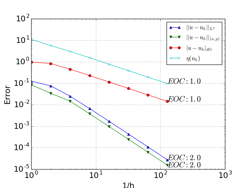
(a) $k=1,p=4$

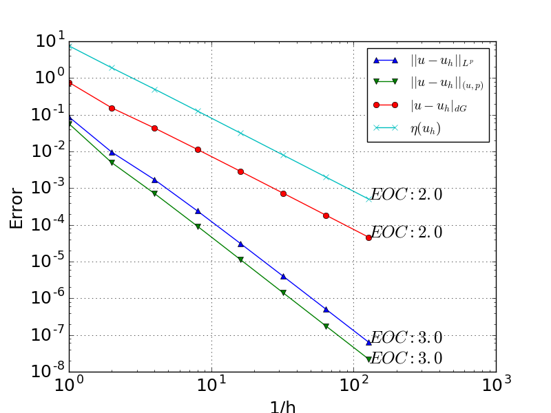
(b) $k=2,p=4$

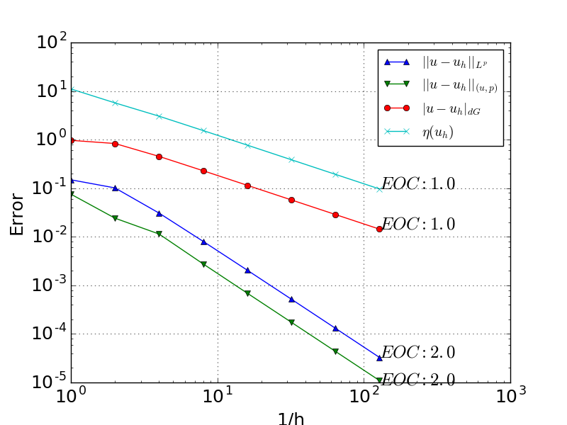
(c) $k=1,p=8$

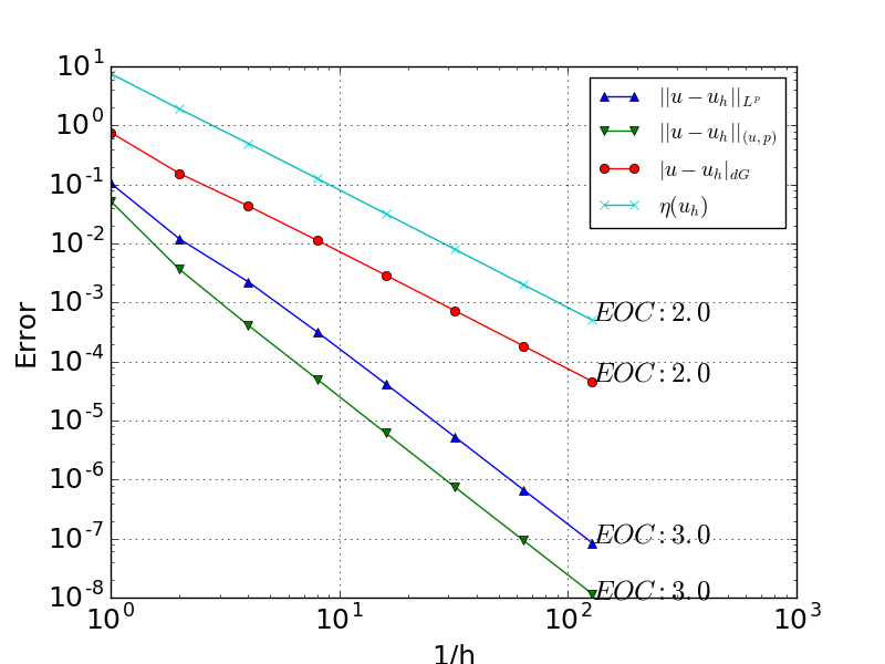
(d) $k=2,p=8$

6.2. Test 2 – Behaviour of an adaptive scheme for various values of $p$

We consider the domain $\Omega=[0,1]^{2}$ and fix $f=1000$ in this case there is no known solution. However, examining the energy functional (1.3) one can see that a minimiser has to ’balance’ the $\operatorname{L}^{2}$ norm of its derivative with the $\operatorname{L}^{p}$ norm of the function. For large $p$ this almost translates into control of the $\operatorname{ess\,sup}$ which causes boundary layers to appear.

We approximate $\Omega$ through a uniformly generated, criss-cross triangular type initial mesh consisting of $4$ elements. We run an adaptive algorithm of SOLVE, ESTIMATE, MARK, REFINE type, where SOLVE consists of solving the formulation (2.11), ESTIMATE is done through the evaluation of the estimator given in Corollary 5.5, MARK is a maximum strategy with $50\%$ of the elements marked for refinement at each iteration and REFINE is a newest vertex bisection.

The results are summarised in Figure 2 (A) – (D) where we consider the case $k=1$, $p=2,4,8,12$ and examine the solution and underlying adaptive mesh.

Figure 2. Solutions of the dG scheme (2.11) for Test 2 and the underlying meshes generated through the adaptive algorithm described in the text. Notice that as $p$ increases, boundary layers become present in the solution requiring mesh resolution to be concentrated at the boundary.

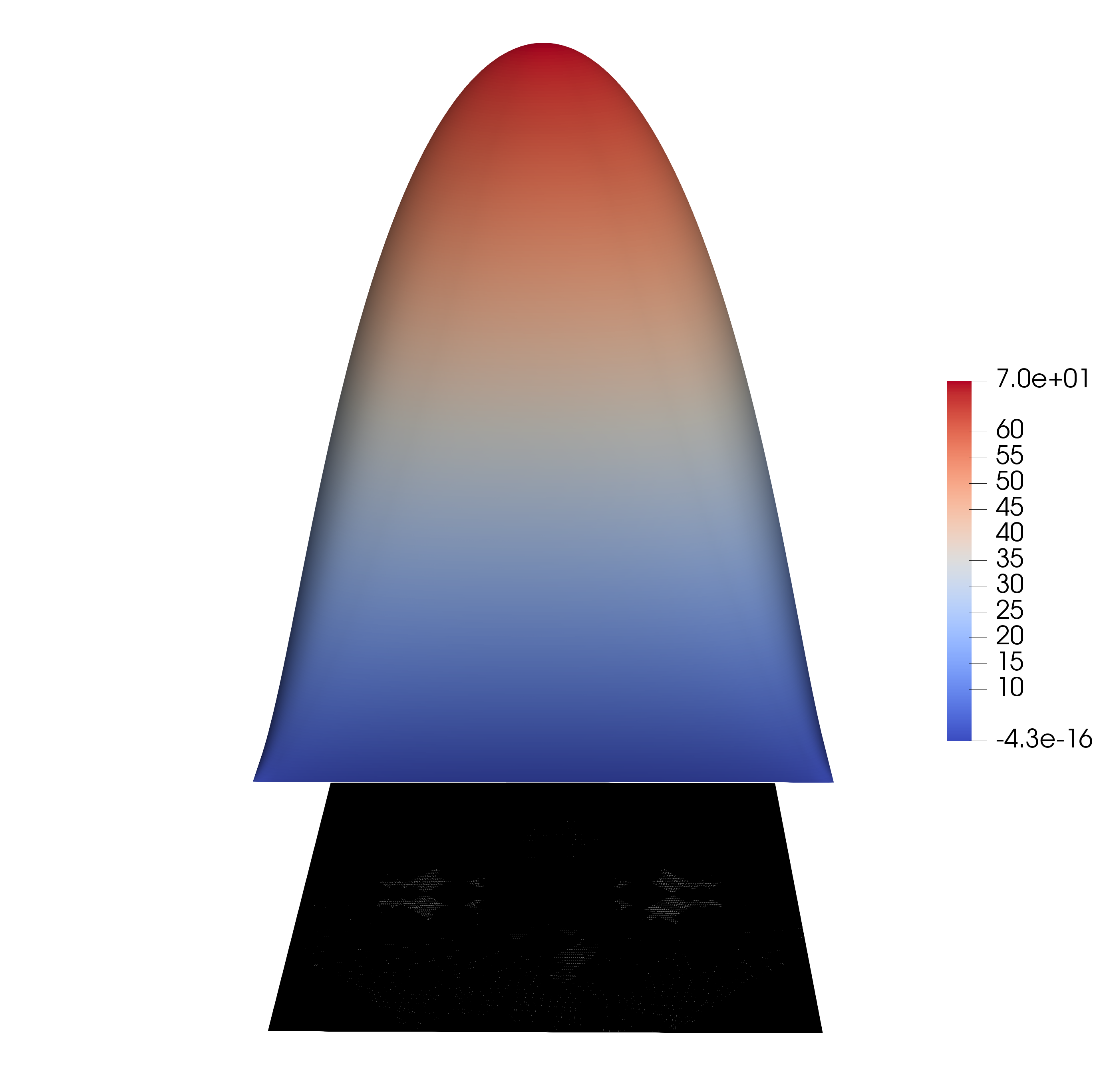
(a) $p=2$. The mesh consists of $924,085$ elements after $13$ iterations.

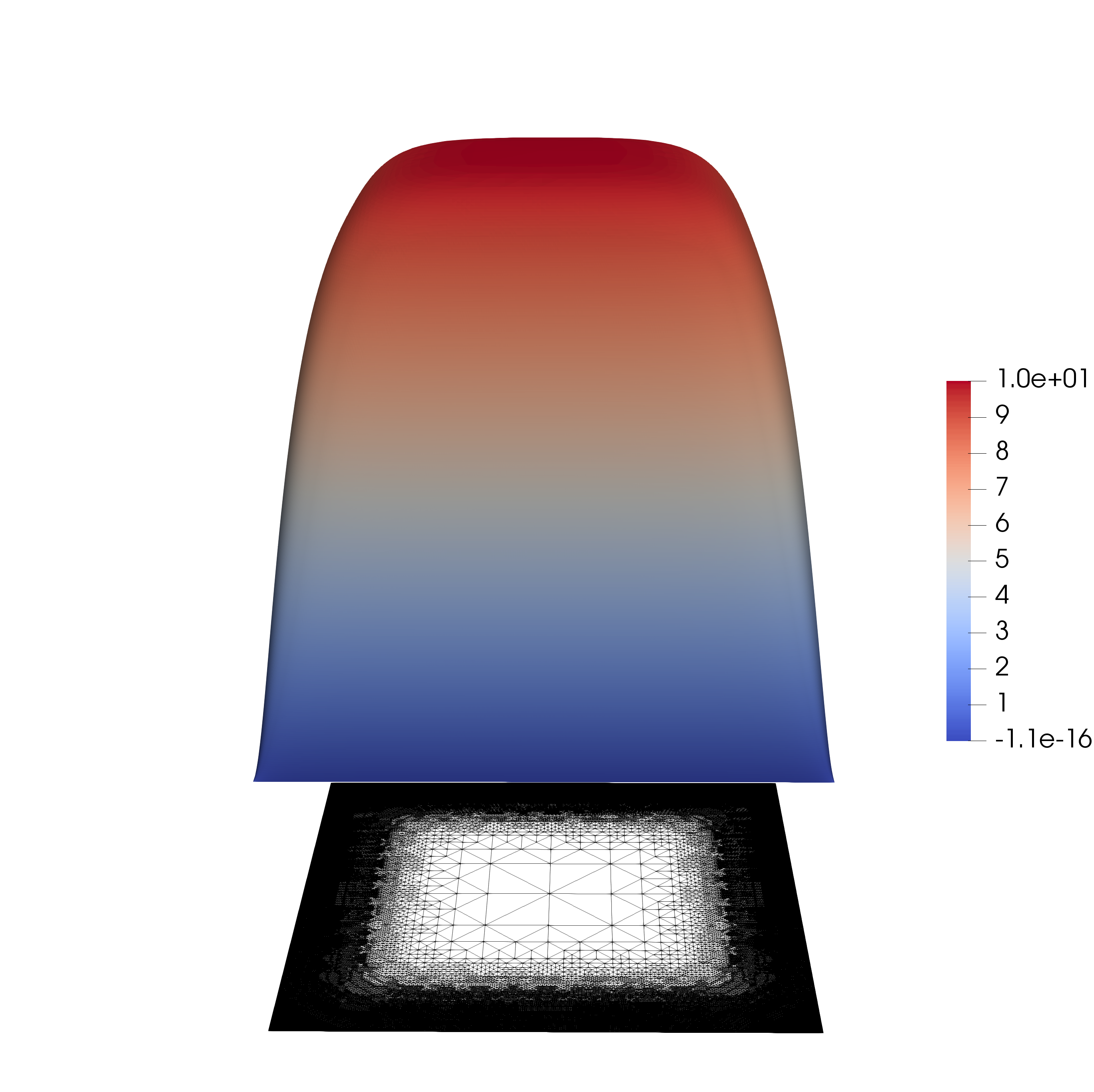
(b) $p=4$. The mesh consists of $361,680$ elements after $13$ iterations.

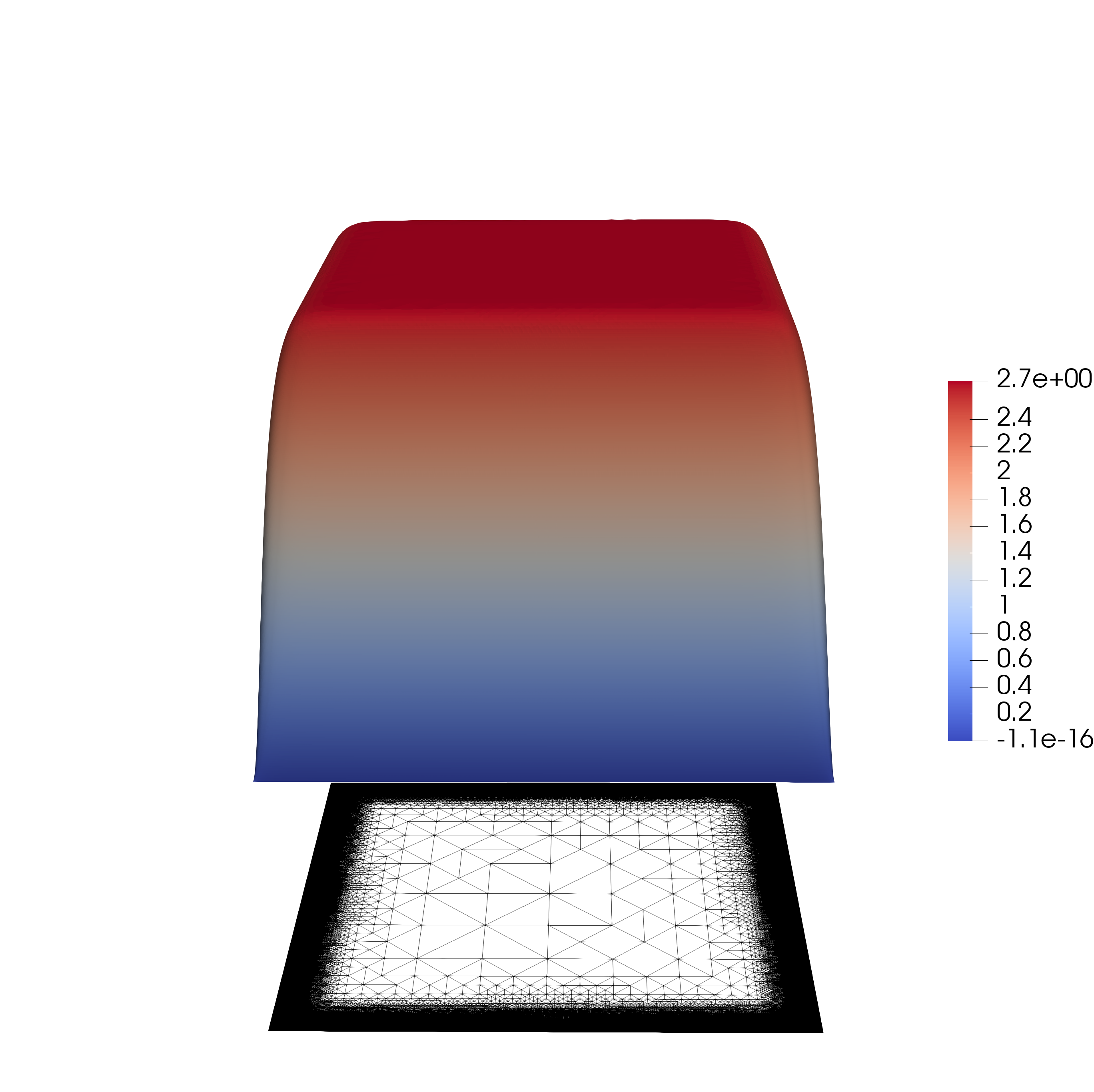
(c) $p=8$. The mesh consists of $339,392$ elements after $13$ iterations.

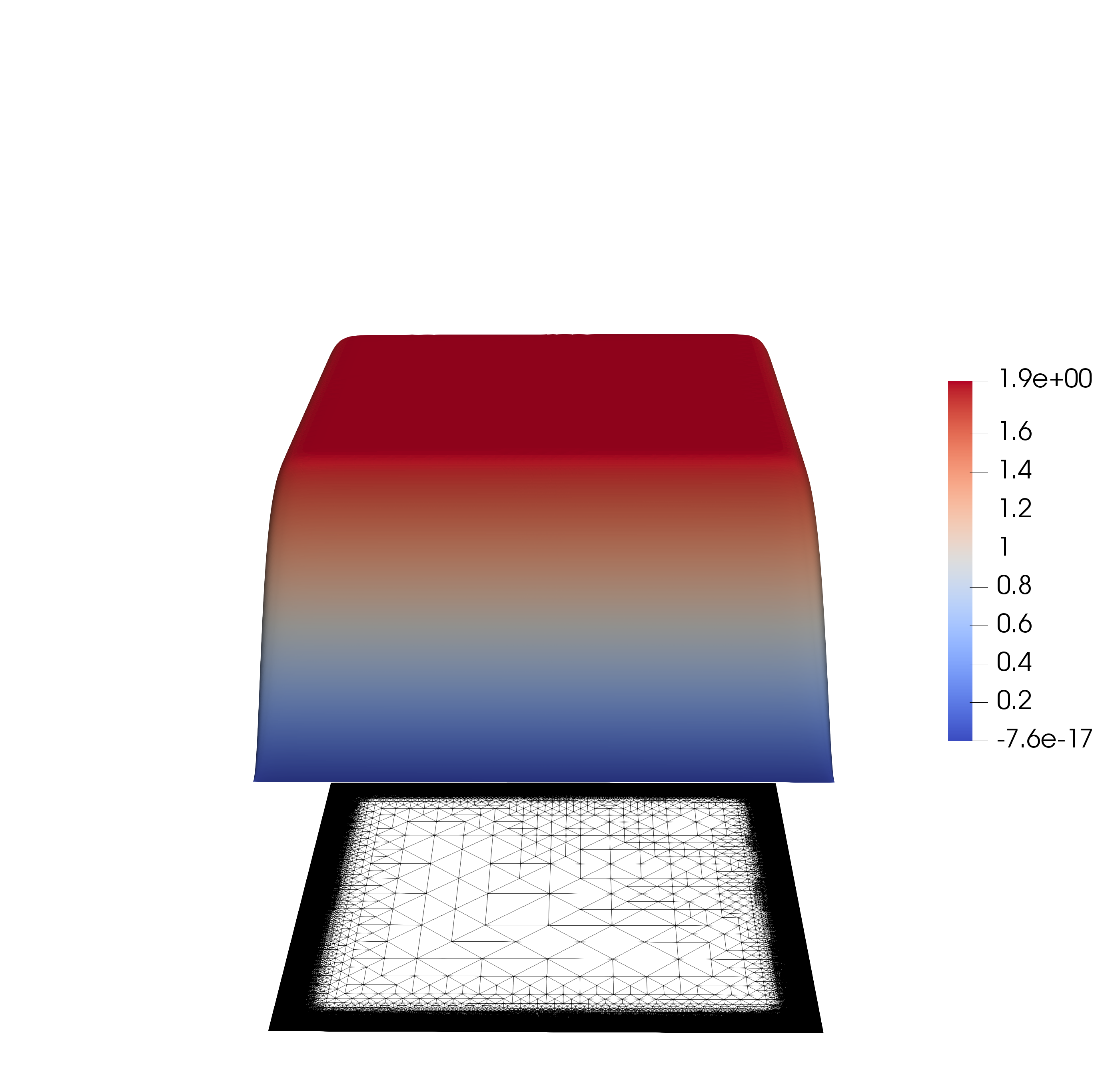
(d) $p=12$. The mesh consists of $340,176$ elements after $13$ iterations.

References

- [CdFM96] Philippe Clément, Djairo Guedes de Figueiredo, and Enzo Mitidieri. Quasilinear elliptic equations with critical exponents. Topological Methods in Nonlinear Analysis, 7(1):133–170, 1996.
- [Cia78] Philippe G. Ciarlet. The finite element method for elliptic problems. North-Holland Publishing Co., Amsterdam, 1978. Studies in Mathematics and its Applications, Vol. 4.
- [EG04] Alexandre Ern and Jean-Luc Guermond. Theory and practice of finite elements, volume 159 of Applied Mathematical Sciences. Springer-Verlag, New York, 2004.
- [EL05] Carsten Ebmeyer and WB Liu. Quasi-norm interpolation error estimates for the piecewise linear finite element approximation of p-Laplacian problems. Numerische Mathematik, 100(2):233–258, 2005.
- [GMP18] Emmanuil Georgoulis, Charalambos Makridakis, and Tristan Pryer. Babuška-Osborn techniques in discontinuous Galerkin methods: -norm error estimates for unstructured meshes. ArXiV preprint: https://arxiv.org/abs/1704.05238, 2018.
- [JP18] James Jackaman and Tristan Pryer. Conservative Galerkin methods for dispersive Hamiltonian problems. arXiv preprint, 2018.
- [JPP18] James Jackaman, Georgios Papamikos, and Tristan Pryer. The design of conservative finite element discretisations for the vectorial modified KdV equation. Applied Numerical Mathematics, 2018.
- [KP03] Ohannes A. Karakashian and Frederic Pascal. A posteriori error estimates for a discontinuous Galerkin approximation of second-order elliptic problems. SIAM J. Numer. Anal., 41(6):2374–2399 (electronic), 2003.
- [KP18] N Katzourakis and T Pryer. On the numerical approximation of -Biharmonic and -Biharmonic functions. To appear in Numerical Methods for Partial Differential Equations, 2018.
- [LB96] WB Liu and John W Barrett. Finite element approximation of some degenerate monotone quasilinear elliptic systems. SIAM journal on numerical analysis, 33(1):88–106, 1996.
- [Pry18] Tristan Pryer. On the finite element approximation of Infinity-Harmonic functions. Proceedings of the Royal Society of Edinburgh Section A: Mathematical and Physical Sciences, 2018.
- [Won75] James SW Wong. On the generalized Emden–Fowler equation. Siam Review, 17(2):339–360, 1975.