Phononic collective excitations in superfluid Fermi gases at nonzero temperatures

Abstract

We study the phononic collective modes of the pairing field $\Delta$ and their corresponding signature in both the order-parameter and density response functions for a superfluid Fermi gas at all temperatures below $T_{c}$ in the collisionless regime. The spectra of collective modes are calculated within the Gaussian Pair Fluctuation approximation. We deal with the coupling of these modes to the fermionic continuum of quasiparticle-quasihole excitations by performing a non-perturbative analytic continuation of the pairing field propagator. At low temperature, we recover the known exponential temperature dependence of the damping rate and velocity shift of the Anderson-Bogoliubov branch. In the vicinity of $T_{c}$, we find analytically a weakly-damped collective mode whose velocity vanishes with a critical exponent of $1/2$, and whose quality factor diverges logarithmically with $T_{c}-T$, thereby clarifying an existing debate in the literature (Andrianov et al. Th. Math. Phys. 28, 829, Ohashi et al. J. Phys. Jap. 66, 2437). A transition between these two phononic branches is visible at intermediary temperatures, particularly in the BCS limit where the phase-phase response function displays two maxima.

I Introduction

Collective excitations are sensitive probes of the microscopic physics of many-body systems. In condensed cold gases, they can be experimentally detected through response functions using for example Bragg spectroscopy. In superfluid paired Fermi gases at zero temperature, they can be classified into several distinctive branches: the Anderson-Bogoliubov (Goldstone) branch Anderson ; Ohashi2003 ; Combescot which has a soundlike dispersion at low momenta according to the Goldstone theorem; the pair-breaking collective branch in the pair-breaking continuum Popov1976 ; KurkjianPB sometimes referred to as Higgs (or Andrianov-Popov) branch; the Leggett branch in multiband systems Leggett . In this work, we focus on the phononic modes, which we characterize in the collisionless regime at non zero temperature.

First predicted by Anderson Anderson within the Random Phase Approximation (RPA), phononic modes have been observed in a series of experiments Bartenstein ; Kinast ; Altmeyer ; Tey ; Sidorenkov ; Hoinka over the last decade and consequently became a subject of intensified theoretical investigation. At zero temperature, the sound velocity Engelbrecht ; Marini ; Diener2008 and later the full spectrum Diener2008 ; Ohashi2003 ; Combescot ; Kurkjian2016 of the Anderson-Bogoliubov branch were investigated theoretically in the Gaussian pair fluctuations (GPF) approximation (equivalent to Anderson’s RPA Kurkjian2017-2 ). The obtained sound velocity agrees with the first sound velocity predicted (in terms of the gas compressibility) by dissipativeless quantum hydrodynamics Khalatnikov1949 . Sophisticated low-energy effective theories were developed to go beyond hydrodynamics and capture the first dispersive correction to the spectrum Manes ; Rupak ; Salasnich2008 , and disagree with GPF/RPA. Finally, the finite lifetime of the phonons at $T=0$ was obtained by considering the Beliaev three-phonon couplings Kurkjian2017 .

At $T\neq 0$, the theory of collective excitations in Fermi gases remains a very open field of investigation, stimulated by its relevance for state-of-the-art experiments. On top of the bosonic couplings Kurkjian2017 ; Escobedo , which are known to cause the temperature dependence of the energy of Bogoliubov quasiparticles Beliaev in a Bose gas, the collective excitations are coupled, in a paired Fermi gas, to the fermionic quasiparticles or “broken pairs” KurkjianPB . The GPF/RPA approximation is able to describe the three-body process of absorption or emission of quasiparticles Ohashi2003 ; Zhang by the collective modes in the collisionless regime: the fermionic quasiparticles are assumed to be non-interacting and thus (in the absence of impurities) to have an infinite relaxation time. Pieri et al. Pieri2004 showed that the exact resonance in the GPF response function, which characterizes the collective mode at $T=0$, is replaced at nonzero temperature by a broadened peak. Calculations of the phonon damping rate were performed in the limit of low temperature Orbach1981 ; Kurkjian2017-2 ; Zou , where it was found to be exponentially small, with an activation energy strictly larger than the gap. Close to the transition temperature, a phononic collective mode was also found Popov1976 and its velocity was predicted to vanish as $(T_{c}-T)^{\alpha}$ with a critical exponent $\alpha=1/2$ according to Ref. Popov1976 and $\alpha=1/6$ according to Ref. Takada1997 .

Collective modes have also been studied in the hydrodynamic limit where the relaxation rate of the quasiparticles is much larger than the frequency of the collective mode, the opposite of the collisionless limit considered here. In neutral Fermi systems, this is done done using two-fluid hydrodynamics Martin1965 which predicts two phononic branches, first and second sound. First sound coincides at $T=0$ with the Anderson-Bogolioubov mode found in collisionless theories but this is no longer the case at $T\neq 0$. First sound velocity remains nonzero at $T_{c}$, unlike the velocity of second sound which vanishes near $T_{c}$ like the superfluid fraction. To describe the damping of these modes, hydrodynamic theories rely on macroscopic dissipation coefficients Hu et al. (2018) (the thermal conductivity and the various viscosities), which have not been calculated theoretically, and are difficult to access experimentally. In charged systems, the phononic nature of the Anderson-Bogoliubov mode is lost at low temperature due to long-range Coulomb interactions that shift its energy toward the plasma energy Anderson . However, in dirty superconductors (which are far in the hydrodynamic regime due to the presence of impurities), it was shown both experimentally Goldman1973 ; Goldman1976 and theoretically Schon1975 ; Volkov1975 ; Volkov1979 that a phononic collective mode, known as the Carlson-Goldman mode exists close to $T_{c}$. The speed and damping rate of this collective mode were found to vanish at $T_{c}$.

In the present work, we compute the complex sound velocity of the phononic collective modes within GPF in a self-consistent nonperturbative way, which allows us to explore all temperatures from $0$ to $T_{c}$. We show that the GPF effective action can be rigorously expanded at low energy $\omega$ and wave number $q$ provided one introduces a complex sound velocity $u$ and sets $\omega=uq$. The expansion yields an explicit equation for $u$ that exhibits a branch cut for real $u$ due to the coupling between phonons and fermionic quasiparticles. Following the procedure of Ref. KurkjianPB for the pair-breaking branch, we solve this equation after analytic continuation through the branch cut, and study the solutions as functions of temperature and interaction strength. In the limits $T\to 0$ and $T\to T_{c}$, we perform this continuation entirely analytically. For intermediate temperatures, we develop a numerical method to perform the analytic continuation, which is based on the procedure of Nozières Nozieres .

We find, in general, two complex roots to the dispersion equation. One root describes the Anderson-Bogoliubov sound velocity in the zero-temperature limit. Near the transition temperature, we find that there exists another phononic collective mode whose complex velocity vanishes with a critical exponent of $1/2$ and whose quality factor diverges logarithmically with $T_{c}-T$. This root appears in both the phase-phase and density-density response functions as a resonance centered around $\omega/v_{\rm F}q\approx\Delta/T_{c}$, which sharpens when approaching $T_{c}$. At intermediary temperature, the two phononic branches coexist, and give a characteristic double-Lorentzian shape (which is accentuated in the BCS regime) to the phase-phase response function.

Our results are in good agreement with the existing experimental data at low temperatures. In the vicinity of $T_{c}$, where the order-parameter collective mode has not yet been observed, we explain how the phase-phase response function could be measured by adapting to cold atoms the setup of Carlson and Goldman based on a Josephson junction between a cold ($T\to 0$) and a hot ($T\to T_{c}$) superfluid.

II Equation for the complex sound velocity

II.1 Gaussian fluctuation action

The present theoretical investigation of collective excitations in superfluid Fermi gases is performed in the path-integral formalism. We consider ultracold two-component Fermi gases with $s$-wave pairing, described deMelo1993 ; Engelbrecht ; Diener2008 by the action functional in Grassmann variables $\left(\bar{\psi}_{\sigma},\psi_{\sigma}\right)$,

$$S=\int_{0}^{\beta}d\tau\int d\mathbf{r}\left[\sum_{\sigma=\uparrow,\downarrow}\bar{\psi}_{\sigma}\left(\frac{\partial}{\partial\tau}-\frac{\nabla_{\mathbf{r}}^{2}}{2m}-\mu\right)\psi_{\sigma}+g\bar{\psi}_{\uparrow}\bar{\psi}_{\downarrow}\psi_{\downarrow}\psi_{\uparrow}\right],$$ (1)

where $\beta=1/T$ is the inverse temperature (we set $\hbar=k_{B}=1$) and the chemical potential $\mu$ fixes the total fermion density. The $s$-wave contact interactions are characterized by the coupling constant $g<0$; the ultraviolet divergence of the contact interaction model is removed by replacing $g$ by the $s$-wave scattering length $a$ through the renormalization relation deMelo1993 :

$$\frac{1}{g}=\frac{m}{4\pi a}-\int\frac{d^{3}k}{\left(2\pi\right)^{3}}\frac{m}{k^{2}}.$$ (2)

The further treatment is based on the effective bosonic pair field action after the Hubbard-Stratonovich transformation with the pair field $\left[\bar{\Psi},\Psi\right]$ and the integration over the fermion fields, as in deMelo1993 ; Engelbrecht ; Diener2008 . This leads to the effective bosonic action $S_{\mathrm{eff}}$ depending on the pair field only:

$$S_{\mathrm{eff}}=-\operatorname{Tr}\ln\left[-\mathbb{G}^{-1}\right]-\int_{0}^{\beta}d\tau\int d\mathbf{r\leavevmode\nobreak\ }\frac{1}{g}\bar{\Psi}\left(\mathbf{r},\tau\right)\Psi\left(\mathbf{r},\tau\right),$$ (3)

where $\mathbb{G}^{-1}\left(\mathbf{r},\tau\right)$ is the inverse Nambu tensor,

$$\mathbb{G}^{-1}\left(\mathbf{r},\tau\right)=\left(\begin{array}[c]{cc}-\frac{\partial}{\partial\tau}+\frac{\nabla_{\mathbf{r}}^{2}}{2m}+\mu&\Psi\left(\mathbf{r},\tau\right)\\ \bar{\Psi}\left(\mathbf{r},\tau\right)&-\frac{\partial}{\partial\tau}-\frac{\nabla_{\mathbf{r}}^{2}}{2m}-\mu\end{array}\right).$$ (4)

In the mean-field approximation, the pair field $\Psi\left(\mathbf{r},\tau\right)$ is replaced by a uniform static order parameter $\Delta$, solution of the mean-field gap equation

$$\int\frac{d^{3}k}{\left(2\pi\right)^{3}}\frac{X\left(E_{\mathbf{k}}\right)}{2E_{\mathbf{k}}}+\frac{1}{g}=0.$$ (5)

Here, $E_{\mathbf{k}}=\sqrt{\xi_{\mathbf{k}}^{2}+\Delta^{2}}$ is the energy of the BCS quasiparticles, with $\xi_{\mathbf{k}}=k^{2}/2m-\mu$ the free fermion energy. The temperature dependence comes in via the function

$$X\left(E_{\mathbf{k}}\right)=\tanh\left(\frac{\beta E_{\mathbf{k}}}{2}\right),$$ (6)

related to the Fermi-Dirac occupation number $n(E_{\mathbf{k}})$ by $X(E_{\mathbf{k}})=1-2n(E_{\mathbf{k}})$. Finally, the mean-field critical temperature $T_{c}=1/\beta_{\mathrm{c}}$ is the temperature at which the order parameter $\Delta$ in Eq. (5) vanishes:

$$\int\frac{d^{3}k}{\left(2\pi\right)^{3}}\frac{\tanh\left(\frac{\beta_{c}\xi_{\mathbf{k}}}{2}\right)}{2\xi_{\mathbf{k}}}+\frac{1}{g}=0.$$ (7)

The Gaussian pair fluctuation approximation consists in expanding the action (3) to second order about the mean-field solution. The pair field $\Psi$ is represented as a sum of the uniform and time-independent value $\Delta$ and the fluctuation field $\varphi$:

$$\Psi\left(\mathbf{r},\tau\right)=\Delta+\varphi\left(\mathbf{r},\tau\right),\quad\bar{\Psi}\left(\mathbf{r},\tau\right)=\Delta+\bar{\varphi}\left(\mathbf{r},\tau\right)$$ (8)

and the fluctuations are taken into account up to second order. Next, the pair field action is rewritten in Fourier space with variables $\left(\mathbf{q},i\Omega_{n}\right)$ where $\Omega_{n}=2\pi n/\beta$ is the bosonic Matsubara frequency. This gives us the quadratic fluctuation action in matrix form:

$$S^{\left(\mathrm{quad}\right)}=\frac{1}{2}\sum_{\mathbf{q},n}\left(\begin{array}[c]{cc}\bar{\varphi}_{\mathbf{q},n}&\varphi_{-\mathbf{q},-n}\end{array}\right)\mathbb{M}\left(\mathbf{q},i\Omega_{n}\right)\left(\begin{array}[c]{c}\varphi_{\mathbf{q},n}\\ \bar{\varphi}_{-\mathbf{q},-n}\end{array}\right),$$ (9)

with the inverse fluctuation propagator $\mathbb{M}\left(\mathbf{q},i\Omega_{n}\right)$. The collective modes of the system are the eigenmodes of the quadratic action (9). The explicit form of the matrix elements of $\mathbb{M}$ with the coupling constant renormalized according to (2) reads:

$$M_{1,1}\left(\mathbf{q},i\Omega_{n}\right) =M_{2,2}\left(-\mathbf{q},-i\Omega_{n}\right)$$

$${=\int\frac{d^{3}k}{\left(2\pi\right)^{3}}\left[\frac{X(E_{\mathbf{k}})}{2E_{\mathbf{k}}}+\frac{X\left(E_{\mathbf{k}}\right)}{4E_{\mathbf{k}}E_{\mathbf{k}+\mathbf{q}}}\right.}$$

$$\times\left(\frac{\left(\xi_{\mathbf{k}}+E_{\mathbf{k}}\right)\left(E_{\mathbf{k}+\mathbf{q}}+\xi_{\mathbf{k}+\mathbf{q}}\right)}{i\Omega_{n}-E_{\mathbf{k}}-E_{\mathbf{k}+\mathbf{q}}}-\frac{\left(\xi_{\mathbf{k}}-E_{\mathbf{k}}\right)\left(\xi_{\mathbf{k}+\mathbf{q}}-E_{\mathbf{k}+\mathbf{q}}\right)}{i\Omega_{n}+E_{\mathbf{k}}+E_{\mathbf{k}+\mathbf{q}}}\right.$$

$$\left.\left.-\frac{\left(\xi_{\mathbf{k}}+E_{\mathbf{k}}\right)\left(\xi_{\mathbf{k}+\mathbf{q}}-E_{\mathbf{k}+\mathbf{q}}\right)}{i\Omega_{n}-E_{\mathbf{k}}+E_{\mathbf{k}+\mathbf{q}}}+\frac{\left(\xi_{\mathbf{k}}-E_{\mathbf{k}}\right)\left(\xi_{\mathbf{k}+\mathbf{q}}+E_{\mathbf{k}+\mathbf{q}}\right)}{i\Omega_{n}+E_{\mathbf{k}}-E_{\mathbf{k}+\mathbf{q}}}\right)\right],$$ (10)

and

$$M_{1,2}\left(\mathbf{q},i\Omega_{n}\right) =M_{2,1}\left(-\mathbf{q},-i\Omega_{n}\right)$$

$$=-\Delta^{2}\int\frac{d^{3}k}{\left(2\pi\right)^{3}}\frac{X\left(E_{\mathbf{k}}\right)}{4E_{\mathbf{k}}E_{\mathbf{k}+\mathbf{q}}}$$

$$\times\left(\frac{1}{i\Omega_{n}-E_{\mathbf{k}}-E_{\mathbf{k}+\mathbf{q}}}-\frac{1}{i\Omega_{n}+E_{\mathbf{k}}+E_{\mathbf{k}+\mathbf{q}}}\right.$$

$$\left.-\frac{1}{i\Omega_{n}-E_{\mathbf{k}}+E_{\mathbf{k}+\mathbf{q}}}+\frac{1}{i\Omega_{n}+E_{\mathbf{k}}-E_{\mathbf{k}+\mathbf{q}}}\right).$$ (11)

Note that the “quasiparticle-quasihole” parts of the matrix coefficients with denominator $i\Omega_{n}\pm\left(E_{\mathbf{k}}-E_{\mathbf{k}+\mathbf{q}}\right)$ vanish at $T=0$ [where $X(E_{\mathbf{k}})=1$] as can be seen by the change of variable $\mathbf{k}\leftrightarrow-\mathbf{k}-\mathbf{q}$, and at $T=T_{c}$ since in this case $E_{\mathbf{k}}=\xi_{\mathbf{k}}$.

II.2 Spectrum of the collective modes

The complex energies $z_{\mathbf{q}}$ of the collective excitations can be determined as the complex poles of the fluctuation propagator $z\mapsto\mathbb{M}^{-1}(q,z)$, or, equivalently, as the complex roots of the determinant of $\mathbb{M}$:

$$\det\mathbb{M}\left(q,z_{\mathbf{q}}\right)=0.$$ (12)

One usually separates in $z_{\mathbf{q}}$ the real part and imaginary part:

$$z_{\mathbf{q}}=\omega_{\mathbf{q}}-i\Gamma_{\mathbf{q}}/2,$$ (13)

where $\omega_{\mathbf{q}}$ is the mode frequency and $\Gamma_{\mathbf{q}}$ its damping rate.

The straightforward analytic continuation of the matrix coefficients (10) and (11) by the replacement $i\Omega_{n}\rightarrow z$ has a branch cut along the whole real axis (unlike in the $T=0$ case KurkjianPB where the branch cut begins at $2\Delta$) due to the denominator $z\pm\left(E_{\mathbf{k}}-E_{\mathbf{k}+\mathbf{q}}\right)$. The roots of Eq. (12), even the low-energy ones, can then only be found when the determinant is analytically continued through the branch cut following the method proposed by Nozières Nozieres ; KurkjianPB . The aim of this paper is to perform this analytic continuation and track the low-energy solutions of (12) in the complex $z$-plane as functions of interaction strength and temperature.

II.3 Equation of state

In dimensionless form, the Gaussian fluctuation matrix $\mathbb{M}$, and hence the collective mode energy $z_{\bf q}$, depend on two reduced parameters: $\Delta/T$ and $\Delta/\mu$, which both depend on temperature. One may want to replace these parameters by more usual quantities such as $T/T_{c}$, and the interaction strength, measured by the product $k_{F}a$ of the scattering length $a$ and Fermi wavevector $k_{F}$. This is done in three steps. First, one uses the number equation to express $\Delta/\epsilon_{F}$ ($\epsilon_{F}$ is the Fermi energy) as a function of $\Delta/T$ and $\Delta/\mu$. The crudest approximation, which can be used only for a qualitative explanation of collective excitations is the mean-field number equation

$$n\equiv\frac{k_{F}^{3}}{3\pi^{2}}{=\int\frac{d^{3}{k}}{(2\pi)^{3}}\left(1-\frac{\xi_{\mathbf{k}}}{E_{\mathbf{k}}}X(E_{\mathbf{k}})\right).}$$ (14)

where $n$ is the average density of the gas. Second, one relates $k_{F}a$ to $\Delta/T$, $\Delta/\mu$ and $\Delta/\epsilon_{\rm F}$ by combining Eqs. (2) and (5):

$$\frac{m}{4\pi a}=\int\frac{d^{3}{k}}{(2\pi)^{3}}\left(\frac{m}{k^{2}}-\frac{X\left(E_{\mathbf{k}}\right)}{2E_{\mathbf{k}}}\right).$$ (15)

With these two equations, one can change the parametrization of $z_{\bf q}$ from ($\Delta/T$,$\Delta/\mu$) to $(k_{\rm F}a,\Delta/\epsilon_{\rm F})$, or equivalently to $(k_{\rm F}a,T/\epsilon_{\rm F})$ using $T/\epsilon_{\rm F}=\Delta/\epsilon_{\rm F}\times T/\Delta$. Third, there remains to express $T_{\rm c}/\epsilon_{\rm F}$ as a function of $k_{\rm F}a$ using Eqs. (14) and (15) specified at $T=T_{c}$, that is for $\Delta=0$: Eq. (14) yields $T_{\rm c}/\epsilon_{\rm F}$ as a function of $\mu(T_{\rm c})/T_{\rm c}$ and Eq. (15) relates this last parameter to $k_{\rm F}a$.

In this process, the mean-field number equation (14) can be replaced by a more accurate one, such as the number the number equation obtained via renormalization group theory Boettcher , the one obtained from Monte Carlo calculations Astr ; Bulgac2006 , or the one extracted from experimental data Salomon2010 ; Zwierlein2012 ; Hoinka . Here we will use more particularly an equation of state which incorporates the Gaussian fluctuations of the order-parameter [Eq. (9)] to the number equation, as proposed in Refs. Nozières and Schmitt-Rink (1985); Diener2008 ; HLD ; HLD1 . This allows us to avoid the aberrant mean-field prediction of a diverging $T_{c}$ in the BEC regime Nozières and Schmitt-Rink (1985). A major issue of these equations of state accounting for Gaussian fluctuations is that they lead to artifacts when using the mean-field gap equation (15) near $T_{c}$ (they loose the $\Delta=O(\sqrt{T_{c}-T})$ critical behavior known from the theory of Ginzburg-Landau and predict an aberrant first order phase transition). As explained in Appendix A, we solve this issue by rescaling the temperature at which the gap equation is used by the ratio of the mean-field and corrected critical temperature (which is a refinement of the idea of Refs. Taylor2008 ; Taylor ). In this way, the zero temperature equation-of-state coincides with the “GPF” scheme of Ref. HLD , the critical temperature is the one computed by Nozières – Schmitt-Rink Nozières and Schmitt-Rink (1985), and the critical behavior $\Delta=O(\sqrt{T_{c}-T})$ (which is crucial for our study of the collective modes) is preserved.

Using an improved equation of state does not qualitatively change our results on the collective modes (it is a mere rescaling of the dependence on $k_{\rm F}a$ and $T/T_{c}$) but makes them more quantitative. This strategy is used in our numeric results for collective excitations, particularly in Secs. IV, VI for the spectra of collective modes and in Sec. VII.2 to compare our results to measurements of the sound velocity.

III Long-wavelength expansion

III.1 Expansion of the $\mathbb{M}$ matrix for phononic energies

In the present treatment, we focus on obtaining an analytic expression of the velocity of the phononic modes in the long-wavelength limit ($q\rightarrow 0$). Their eigenenergy is expected to behave as $z_{\mathbf{q}}\sim u_{\mathrm{s}}q$, with the complex sound velocity $u_{\mathrm{s}}$. The sound velocity was calculated at $T=0$ Marini ; Salasnich ; Diener2008 where the quasiparticle-quasihole branch cut vanishes such that $u_{\mathrm{s}}$ is real and the long-wavelength expansion of the matrix elements $M_{j,k}\left(\mathbf{q},z\right)$, $j,k=1,2$ presents no difficulty, i. e., the two-dimensional expansion in powers of $q$ and $z$ can be done successively. Predictions of the limiting behavior at the transition temperature ($T\to T_{c}$) are also available Popov1976 ; Takada1997 at weak coupling, and will be discussed in section V.

For $0<T<T_{c}$, the point $(q=0,z=0)$ is a branch point of $\det\mathbb{M}$ and different limiting values when $(q,z)\rightarrow(0,0)$ can be obtained depending on the path followed in the $(q,z)$ hyperplane. Therefore, there exists no Taylor expansion valid everywhere in a vicinity of the point $(q=0,z=0)$ Engelbrecht . An expansion can be obtained nonetheless assuming that $q$ and $z$ are small yet proportional to each other. Consequently, we set $z\equiv uq$, where $u$ is a complex number independent of $q$. An analogous trick was performed in Ref. Kosztin .

In the $q\rightarrow 0$ limit, it is more tractable to express the matrix elements (10) and (11) in the modulus-phase basis,

$$\tilde{\mathbb{{M}}}\left(\mathbf{q},z\right)=\left(\begin{array}[c]{cc}{M}_{--}\left(\mathbf{q},z\right)&{M}_{+-}\left(\mathbf{q},z\right)\\ {M}_{-+}\left(\mathbf{q},z\right)&{M}_{++}\left(\mathbf{q},z\right)\end{array}\right),$$ (16)

where the new matrix elements are obtained by the unitary transformation Engelbrecht :

$${M}_{++}\left(\mathbf{q},z\right) =\frac{M_{1,1}\left(\mathbf{q},z\right)+M_{1,1}\left(\mathbf{q},-z\right)}{2}-M_{1,2}\left(\mathbf{q},z\right),$$ (17)

$${M}_{--}\left(\mathbf{q},z\right) =\frac{M_{1,1}\left(\mathbf{q},z\right)+M_{1,1}\left(\mathbf{q},-z\right)}{2}+M_{1,2}\left(\mathbf{q},z\right),$$ (18)

$${M}_{+-}\left(\mathbf{q},z\right) =\frac{M_{1,1}\left(\mathbf{q},z\right)-M_{1,1}\left(\mathbf{q},-z\right)}{2}=-{M}_{-+}\left(\mathbf{q},z\right).$$ (19)

The diagonal matrix elements ${M}_{++}\left(\mathbf{q},z\right)$ and ${M}_{--}\left(\mathbf{q},z\right)$ correspond to the phase and modulus fluctuations, respectively. The nondiagonal matrix elements describe mixing of modulus and phase fluctuations. The series expansion in powers of $q$ in this basis gives:

$${M}_{++}(\mathbf{q},uq)\! = \!\frac{q^{2}}{2m\Delta}\frac{m_{++}(u)}{\Delta}+O(q^{4}),$$ (20)

$${M}_{--}(\mathbf{q},uq)\! = \frac{m_{--}(u)}{\Delta}+O(q^{2}),$$ (21)

$${M}_{+-}(\mathbf{q},uq)\! = \!\frac{uq}{\Delta}\frac{m_{+-}(u)}{\Delta}+O(q^{3}),$$ (22)

with coefficients (dimensionless except for the Jacobian $d^{3}k$):

$$m_{++}(u) = \int\frac{\Delta^{2}d^{3}{k}}{(2\pi)^{3}}\left[\frac{e_{c}(v_{\bf k})}{6}\left(\frac{X(E_{\bf k})}{E_{\bf k}^{3}}-\frac{X^{\prime}(E_{\bf k})}{E_{\bf k}^{2}}\right)-\frac{e_{c}(u)}{2}\frac{X(E_{\bf k})}{E_{\bf k}^{3}}\right.$$ (23)

$$\left.\qquad\qquad\qquad\qquad\quad+e_{c}(u)\frac{\Delta^{2}}{2{E}_{\bf k}^{2}}\frac{X^{\prime}(E_{\bf k})e_{c}(v_{\bf k})\cos^{2}\theta}{({E}_{\bf k}^{2}e_{c}({u})-{\xi}_{\bf k}^{2}e_{c}(v_{\bf k})\cos^{2}\theta)}\right],$$

$$m_{--}(u) = \int\frac{\Delta^{3}d^{3}{k}}{(2\pi)^{3}}\left[\frac{X(E_{\bf k})}{2{E}_{\bf k}^{3}}+\frac{{\xi}_{\bf k}^{2}}{2{E}_{\bf k}^{2}}\frac{X^{\prime}(E_{\bf k})e_{c}(v_{\bf k})\cos^{2}\theta}{({E}_{\bf k}^{2}e_{c}({u})-{\xi}_{\bf k}^{2}e_{c}(v_{\bf k})\cos^{2}\theta)}\right],$$ (24)

$$m_{+-}(u) = \int\frac{\Delta^{2}d^{3}{k}}{(2\pi)^{3}}\left[-\frac{{\xi}_{\bf k}X(E_{\bf k})}{4{E}_{\bf k}^{3}}+\frac{\Delta{\xi}_{\bf k}}{4{E}_{\bf k}^{2}}\frac{\Delta X^{\prime}(E_{\bf k})e_{c}(v_{\bf k})\cos^{2}\theta}{({E}_{\bf k}^{2}e_{c}({u})-{\xi}_{\bf k}^{2}e_{c}(v_{\bf k})\cos^{2}\theta)}\right].$$ (25)

Here $v_{\bf k}=k/m$ is the phase velocity associated to wave vector $k$, and $e_{c}(v)=mv^{2}/2$ is the kinetic energy associated to velocity $v$.

III.2 Reduced dispersion equation

Substituting the series expansions of the matrix elements into the determinant of $\mathbb{\tilde{M}}$, we get

$$\det\mathbb{\tilde{M}}\left(\mathbf{q},z=uq\right)={W\left(u\right)}\frac{q^{2}}{2m\Delta^{3}}+O\left(q^{4}\right),$$ (26)

where the function $W\left(u\right)$ is given by:

$$W\left(u\right)=m_{++}(u)m_{--}(u)-\frac{2mu^{2}}{\Delta}m_{+-}^{2}(u),$$ (27)

Let $u_{\mathrm{s}}$ be a generic solution of the low-$q$ dispersion equation:

$$W\left(u_{\mathrm{s}}\right)=0.$$ (28)

The real part of $u_{\mathrm{s}}$ is readily interpreted as a sound velocity

$$c_{\mathrm{s}}\equiv\text{$\operatorname{Re}$}\left(u_{\mathrm{s}}\right)=\lim_{q\rightarrow 0}\frac{\omega_{q}}{q}$$ (29)

and the imaginary part

$$\kappa_{\mathrm{s}}\equiv\operatorname{Im}\left(u_{\mathrm{s}}\right)=\lim_{q\rightarrow 0}\frac{\Gamma_{q}}{2q}$$ (30)

gives access to the long-wavelength limit of an inverse quality factor $\Gamma_{q}/\omega_{q}$:

$$\frac{2\kappa_{\mathrm{s}}}{c_{\mathrm{s}}}=\lim_{q\rightarrow 0}\frac{\Gamma_{q}}{\omega_{q}}.$$ (31)

As such, the reduced dispersion equation (28) has no root: none on the real axis ($u\in\mathbb{R}$) which is entirely spanned by the branch cut caused by the resonant denominator in Eqs. (23–25), and none either in the lower complex plane ($\textrm{Im}\,u<0$), otherwise there would also exist an unstable solution in the upper plane (since $W(u)=0\implies W(-u)=0$). Two distinct strategies can be adopted to overcome this apparent paradox.

$(i)$ One can limit the study to the vicinity of the real axis setting $u=c+i0^{+}$ with $c\in\mathbb{R}$, and study the various responses of the system as a function of $c$. Although the response functions (defined in the next subsection) have no pole, they may exhibit resonance peaks whose position and width may be fitted to extract the real and imaginary parts of a phenomenological speed of sound. This corresponds to an experiment where the response of the gas is recorded at fixed (and low) $q$ as a function of $\omega$, using for example Bragg spectroscopy Hoinka . The disadvantage of this strategy is that it relies on a delicate choice of a fitting function Takada1997 for $1/W(c+i0^{+})$, in particular in the case (that we will encounter) where the function has more than one peak.

$(ii)$ One can instead look for true solutions of the dispersion equation (28) in the analytic continuation through the branch cut. Knowledge of the poles of $1/W(u)$ in the complex plane makes it easy to devise an analytic approximation for the response functions. It also allows for a clear definition of the speed of sound, and therefore for a rigorous study of its temperature dependence, and in particular of its critical exponent near $T_{c}$.

III.3 Response functions

The response functions of the pair field in the GPF approximation are the coefficients of the propagator $\mathbb{\tilde{M}}^{-1}$ evaluated on the real axis $z=\omega+i0^{+}$ Minguzzi et al. (2001) (hence without analytic continuation through the branch cut). In the low-$q$ limit, $\tilde{\mathbb{{M}}}^{-1}\left(\mathbf{q},z\right)$ is given by:

$$\frac{{q}^{2}}{2m}\mathbb{\tilde{M}}^{-1}\left(\mathbf{q},uq\right)=\frac{\Delta}{W\left(u\right)}\left(\begin{array}[c]{cc}m_{++}(u)\frac{q^{2}}{2m}&-m_{+-}(u)uq\\ -m_{+-}(u)uq&\Delta m_{--}(u)\end{array}\right)+O\left(q^{4}\right).$$ (32)

The largest response is thus in the phase-phase propagator $[\tilde{\mathbb{{M}}}^{-1}]_{2,2}$. We define

$$\chi(c)\equiv\lim_{q\rightarrow 0}\frac{1}{\pi}\operatorname{Im}\left\{\frac{q^{2}}{2m\Delta^{2}}[\mathbb{\tilde{M}}^{-1}]_{2,2}(\mathbf{q},(c+i0^{+})q)\right\}=\frac{1}{\pi}\operatorname{Im}\frac{m_{--}\left(c+i0^{+}\right)}{W\left(c+i0^{+}\right)},$$ (33)

the phase-phase response as a function of the velocity $c=\omega/q\in\mathbb{R}$.

To account for density excitations, one should supplement the quadratic action (9) by an auxiliary action containing the exciting density fields, which we do in Appendix C. The result is the following expression of the retarded density-density Green’s function

$${G}_{\rho}^{R}\left(\mathbf{q},\omega+i0^{+}\right) ={M}_{\rho\rho}\left(\mathbf{q},\omega\right)$$

$$-\left\{\left[{M}_{-\rho}\left(\mathbf{q},\omega\right)\right]^{2}\frac{{M}_{++}\left(\mathbf{q},\omega\right)}{\det\mathbb{\tilde{M}}\left(\mathbf{q},\omega\right)}+\left[{M}_{+\rho}\left(\mathbf{q},\omega\right)\right]^{2}\frac{{M}_{--}\left(\mathbf{q},\omega\right)}{\det\mathbb{\tilde{M}}\left(\mathbf{q},\omega\right)}\right.$$

$$\left.-2{M}_{-\rho}\left(\mathbf{q},\omega\right){M}_{+\rho}\left(\mathbf{q},i\Omega_{m}\right)\frac{{M}_{+-}\left(\mathbf{q},\omega\right)}{\det\mathbb{\tilde{M}}\left(\mathbf{q},\omega\right)}\right\}.$$ (34)

which is in agreement with Eq. (20) of Ref. Minguzzi et al. (2001) (taking the density-density element of the response function matrix). The density-pairing field and density-density elements of the fluctuation matrix, $M_{\pm\rho}$ and $M_{\rho\rho}$, (and their low-$q$ expansion) are given explicitly in Appendix C. We then define the low-$q$ density-density response function as

$$\chi_{\rho}\left(c\right)=-\frac{1}{\pi}\lim_{q\rightarrow 0}\left[\operatorname{Im}G_{\rho}^{R}\left(\mathbf{q},\left(c+i0^{+}\right)q\right)\right].$$ (35)

It is related to the long wavelength density-density response function by $\lim_{q\rightarrow 0}S(\textbf{q},cq)=\chi_{\rho}\left(c\right)/(1-e^{-\beta cq})$. $\chi_{\rho}$ is composed of two terms which have a distinct physical origin

$$\chi_{\rho}\left(c\right)=\chi_{\rho}^{\left(1\right)}\left(c\right)+\chi_{\rho}^{\left(2\right)}\left(c\right),$$ (36)

The first term,

$$\chi_{\rho}^{\left(1\right)}\left(c\right)=-\frac{1}{\pi}\lim_{q\rightarrow 0}\left[\operatorname{Im}{M}_{\rho\rho}\left(\mathbf{q},\left(c+i0^{+}\right)q\right)\right]$$ (37)

does not disappear at $T_{c}$; above it, it describes the known density response of free fermions. The second contribution $\chi_{\rho}^{\left(2\right)}$ gathers the terms between curly brackets in (34), which have the determinant of $\tilde{\mathbb{M}}$ (the pairing field fluctuation matrix) in the denominator. It describes the contribution of the pairing field to the density response and it is specific to the superfluid phase. Due to the $\det\mathbb{\tilde{M}}$ in the denominator of this term, it has the same poles and thus the same collective modes as the pair field response function.

IV Low-temperature behavior

We briefly study the behavior of the speed of sound at zero and low temperature, which are overall well established results. At $T=0$, one has $X(E_{k})=1$ and $X^{\prime}(E_{k})=0$ such that the coefficients (23–25) of the $\left(q,z\right)$ expansion depend trivially on $u$ (as expected since the singular “quasiparticle-quasihole” terms vanish). The dispersion equation (28) in this case has one real root $u_{\mathrm{s,0}}(T=0)=c_{\mathrm{s,0}}(T=0)$ which satisfies the hydrodynamic formula $mc_{\mathrm{s,0}}^{2}=nd\mu/dn$ Martin1965 ; Taylor and can thus be unambiguously identified as the first sound of two-fluid hydrodynamics. At low but non zero temperatures ($T\ll\Delta$, $T\ll T_{c}$), the root $u_{\mathrm{s1}}$ acquires an imaginary part exponentially small in temperature, $\textrm{Im}\,u_{s,0}(T)\propto e^{-\Delta^{\prime}/T}$, with an activation energy $\Delta^{\prime}$ strictly larger than $\Delta$ Orbach1981 . This is because the fermionic quasiparticles of energy $\Delta$ have zero group velocity, and thus cannot contribute to the damping. Our results for this imaginary part are in agreement with Refs. Orbach1981 ; Kurkjian2017-2 and with Landau roton-phonon theory Kurkjian2017-3 . The collective mode also acquires a velocity shift $\delta c_{s,0}(T)=\textrm{Re}\,u_{s,0}(T)-c_{s,0}(0)$. In the weak-coupling BCS limit, we agree with Kulik et al. Orbach1981 who predicted an exponentially small increase of the velocity:

$$\delta c_{s,0}(T)\stackrel{{\scriptstyle[}}{{T}}\to 0]{1/k_{F}a\to-\infty}{=}\frac{2v_{\rm F}}{5\sqrt{3}}\sqrt{\frac{2\pi T}{\Delta}}e^{-\Delta/T}.$$ (38)

As shown in Fig. 1, we find that after this exponential increase, the velocity passes through a shallow maximum and then decreases. This behavior is reminiscent of what Ref. Escobedo obtained with a low-energy effective theory. On the contrary, in the BEC regime, we find that the velocity shift is always negative.

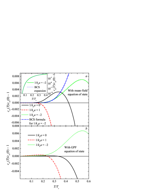
Figure 1: (Color online) (a) Relative correction to the sound velocity $c_{\mathrm{s}1}$ at low temperatures $T\ll\Delta$, calculated using the mean-field equation of state at unitarity ($1/|a|=0$ solid curve), in the BEC regime ($1/k_{F}a=1$, dashed red curve) and in the BCS regime ($1/k_{F}a=-2$, green dashed curve). This last curve is compared to the low-temperature exponential formula of Orbach1981 , (blue dashed-dotted curve), also in the inset in logarithmic scale. (b) These corrections calculated using the GPF equation of state.

V Behavior near the critical temperature

In contrast with the low-temperature regime, the behavior of the collectives branches near $T_{c}$ remains a controversial problem. The available predictions neatly contradict themselves: Popov and Andrianov Popov1976 find the pure imaginary dispersion relation

$$\omega_{q}=-i\frac{7\zeta(3)v_{\rm F}q}{6\pi^{3}T_{c}}\left(\sqrt{4\Delta^{2}+v_{\rm F}^{2}q^{2}}+2\Delta\right),$$ (39)

which indicates that $u_{s}(T)$ has a critical exponent of $1/2$, that is, $u_{s}(T)\underset{(T_{c}-T)\to 0}{\sim}a\Delta\sim a^{\prime}(T_{c}-T)^{1/2}$ with $a,a^{\prime}\in i\mathbb{R}$. In contradiction with this result, Ohashi and Takada Takada1997 predict a real speed of sound with a critical exponent of $1/6$, that is, $u_{s}(T)\underset{(T_{c}-T)\to 0}{\sim}b(T_{c}-T)^{1/6}$, $b\in\mathbb{R}$. These two studies are limited to the weak coupling regime $1/k_{\rm F}a\to-\infty$. More recent studies dealing with the strong coupling regime Kosztin confirmed the cancellation of the speed of sound at $T_{c}$ (irrespectively of the interaction regime) but did not predict its critical exponent. Using our dispersion equation (28), we are in a good position to solve this controversy.

Using the mean-field equation of state (or the “scaled GPF” scheme described in Appendix A, which preserves this limiting behavior), the limit $T\to T_{c}$ implies

$$\epsilon \equiv \frac{\Delta}{T}=O(\sqrt{T_{c}-T}),$$ (40)

$$\frac{\mu}{T} = \frac{\mu(T_{c})}{T_{c}}+O(T_{c}-T).$$ (41)

Neglecting terms of order $\epsilon^{2}$, we thus take the limit $\epsilon\to 0$ for $\mu/T$ fixed to $m_{c}\equiv{\mu(T_{c})}/{T_{c}}$. Note that $m_{c}$ is related to $k_{\rm F}a$ by an equation of state at $T_{c}$, as explained in section II.3. This relation is of course different for, e. g., the mean-field or scaled GPF equations of state.

V.1 Regimes with ($\mu>0$)

When $\mu(T_{c})>0$ (that is for $1/k_{\rm F}a<0.68$ with the mean-field equation-of-state), the $m_{\sigma\sigma^{\prime}}$ coefficients in the limit $\epsilon\to 0$ become

$$\frac{\check{m}_{++}}{m_{c}} = \check{u}^{2}{F(\check{u})}+\epsilon f(m_{c})+O(\epsilon^{2})$$ (42)

$$\check{m}_{--} = \epsilon\left[G(\check{u})+\epsilon g(m_{c})\right]+O(\epsilon^{3})$$ (43)

$$\check{m}_{+-} = {\epsilon}h(m_{c})+O(\epsilon^{2})$$ (44)

Since $\mu$ is the most convenient energy scale near $T_{c}$, we have redimensionalized the speed of sound, $\check{u}^{2}=mu^{2}/2\mu$, and the integrals in consequence, $m_{\sigma\sigma^{\prime}}={\rho(\mu)\Delta}\check{m}_{\sigma\sigma^{\prime}}/{2}$, where $\rho(\mu)=\sqrt{2m^{3}\mu}/\pi^{2}\hbar^{3}$ is the density of states at energy $\mu$ (setting the volume of the gas equal to unity). We also introduced the functions

$$F(\check{u}) = -\frac{\pi}{8}\left(\sqrt{1-\frac{1}{\check{u}^{2}}}+\check{u}\,\textrm{arccsc}(\check{u})\right)$$ (45)

$$G(\check{u}) = \frac{\pi}{4}{\check{u}\,\textrm{arccsc}(\check{u})}$$ (46)

and we recall that $\textrm{arccsc}(z)=-i\textrm{ln}\left(\sqrt{1-\frac{1}{z^{2}}}+\frac{i}{z}\right)$. Functions $f$, $g$ and $h$ of $m_{c}$ are defined in Appendix B where the derivation is detailed. The dispersion equation (28) on $\check{u}$ then becomes

$$\left[{\check{u}^{2}}F(\check{u})+\epsilon f(m_{c})\right]\left[G(\check{u})+\epsilon g(m_{c})\right]-4{\check{u}^{2}}h^{2}(m_{c})=0$$ (47)

This equation should be solved in the lower-half complex plane after analytic continuation of the functions $F$ and $G$. With the analytic formulas Eqs. (45,46), this is simply done by the replacements $\sqrt{1-{1}/{\check{u}^{2}}}\to-\sqrt{1-{1}/{\check{u}^{2}}}$ and $\textrm{arccsc}(\check{u})\to\pi-\textrm{arccsc}(\check{u})$. Remarkably, we find that the analytically continued equation has in fact two solutions. The first one (shown in Fig. 2 as a function of $m_{c}$ or $1/k_{\rm F}a$) has a nonzero limit when $\epsilon\to 0$; it is given by the transcendent equation

$$F(\check{u}_{s1})G(\check{u}_{s1})=4h^{2}(m_{c})$$ (48)

The second solution $u_{s2}$ behaves as $\epsilon\propto(T_{c}-T)^{1/2}$, which confirms the $1/2$ critical exponent predicted by Andrianov and Popov. Setting $\check{u}_{s2}=\epsilon\,\bar{u}_{s2}$, and simplifying Eq. (47) for $\epsilon\ll 1$ (but $|\textrm{ln}\,\epsilon|=O(1)$) we obtain

$$\left(-i\frac{\pi\bar{u}_{s2}}{8}+{f(m_{c})}\right)\left(\vphantom{\frac{\check{u}^{2}}{2}}\frac{\pi\bar{u}_{s2}}{4}\left[\pi+i\textrm{ln}\frac{i\bar{u}_{s2}\epsilon}{2}\right]+g(m_{c})\right)-4{\bar{u}_{s2}^{2}}h^{2}(m_{c})=0$$ (49)

Thus, $\bar{u}_{s2}$ still depends logarithmically on $\epsilon$. This dependence can in turn be expanded at temperatures extremely close to $T_{c}$, that is for $|\textrm{ln}\,\epsilon|\gg 1$:

$$\check{u}_{s2}=\epsilon\frac{8f(m_{c})}{\pi}\left(-i\left[1+\frac{128h^{2}(m_{c})}{\pi^{2}|\textrm{ln}\epsilon|}\right]+\frac{\gamma}{\textrm{ln}^{2}\epsilon}\right)+O\left(\frac{\epsilon}{\textrm{ln}^{3}\epsilon}\right)$$ (50)

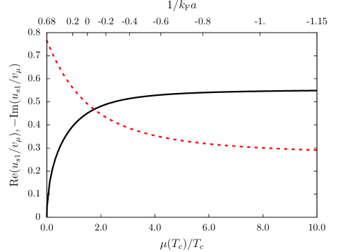
Figure 2: (Color online) The first root $u_{s1}$ of the dispersion equation (47) is plotted, in units of $v_{\mu}=\sqrt{2\mu/m}$, as a function of ${\mu(T_{c})}/{T_{c}}$ (related by the equation of state to the interaction strength $1/k_{\rm F}a$, shown on the top $x$-axis)

The first two terms of this expansion are pure imaginary numbers, while the term in $O(\epsilon/\textrm{ln}^{2}\epsilon)$ has a non-zero real part. The quality factor $\textrm{Re}\,{u}_{s2}/2\textrm{Im}\,{u}_{s2}$ thus vanishes near $T_{c}$ as $\gamma/2\textrm{ln}^{2}\epsilon$, where the coefficient $\gamma$ is:

$$\gamma=-\frac{2^{12}h^{2}}{\pi^{4}}\left[i\frac{\pi}{8}\left\{g+\frac{2^{8}}{\pi^{2}}h^{2}f-2if\left(\pi+i\ln\frac{4f}{\pi}\right)\right\}-64i\frac{h^{2}f}{\pi}\right]$$ (51)

with the short-hand notation $f=f(m_{c})$, $g=g(m_{c})$ and $h=h(m_{c})$.

In the BCS limit ($m_{c}\to+\infty$ or $1/k_{\rm F}a\to-\infty$), one has $h=0$ in (47), such that the dispersion equation becomes $m_{++}m_{--}=0$, and $u_{s1}$ and $u_{s2}$ solve $m_{++}=0$ (while $m_{--}=0$ gives the pair-breaking Popov-Andrianov-“Higgs” mode Popov1976 ; KurkjianPB ). Using the limiting value $f(+\infty)=7\zeta(3)/12\pi^{2}$, we get an expression of ${u}_{s2}$ that agrees with Andrianov-Popov, Eq. (39):

$$\frac{u_{s2}}{v_{\rm F}}\stackrel{{\scriptstyle[}}{{\epsilon}}\to 0]{1/k_{\rm F}a\to-\infty}{=}-i\frac{14\zeta(3)}{3\pi^{3}}\frac{\Delta}{T_{c}},$$ (52)

Conversely, ${u}_{s1}$ has the finite nonzero limit

$$\frac{u_{s1}}{v_{\rm F}}\stackrel{{\scriptstyle[}}{{\epsilon}}\to 0]{1/k_{\rm F}a\to-\infty}{\simeq}0.555-0.266i$$ (53)

The existence of two solutions to the speed-of-sound equation, and thus of two phononic branches, is surprising but it is not an artifact of our analytic continuation scheme. It is confirmed by looking at the response function $\chi(c)$, which is a physical observable. Expressions (42-44) can be used to express the response function near $T_{c}$:

$$\check{\chi}(\check{c})=\frac{1}{\pi m_{c}}\textrm{Im}\,\frac{G(\check{c})+\epsilon g}{(\check{c}^{2}F(\check{c})+\epsilon f)(G(\check{c})+\epsilon g)-4\check{c}^{2}h^{2}}$$ (54)

where the redimensionalization is $\check{\chi}={\chi}\times\left[\rho(\mu)\Delta/2\right]$. In Fig. 3, we show this response function in the far BCS regime $1/k_{\rm F}a=-2$ (corresponding to $\mu(T_{c})/T_{c}\simeq 37.73$). The second root, whose quality factor diverges when $T\to T_{c}$, translates into a sharp resonance peak whose center tends to $c=0$ and whose width vanishes at $T_{c}$. The first root, which conversely has a finite quality factor, does not lead to the appearance of a second peak at temperatures close to $T_{c}$ (we shall see that it does at lower temperatures); it is nevertheless observable in the form of a broad upper shoulder that extends to higher $c$.

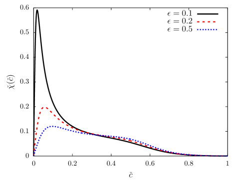
Figure 3: (Color online) The phase-phase response function $\chi$ is plotted as a function of the reduced velocity $\check{c}=c\sqrt{m/2\mu}$ in the far BCS regime, at $1/k_{F}a=-2$ and temperatures $T/T_{c}=0.999$ ($\epsilon=0.1$), $T/T_{c}=0.996$ ($\epsilon=0.2$), and $T/T_{c}=0.97$ ($\epsilon=0.5$). Far from $T_{c}$, the two roots $\check{u}_{s1}$ and $\check{u}_{s2}$ of the dispersion equation have comparable imaginary parts (and comparable residues), which results in a response function with a double bump structure (blue curve). As the temperature is reduced, $\check{u}_{s2}$, whose real and imaginary part tend to $0$ like $\epsilon$, dominates, which results in the large resonance peak near $c=0$ (black curve). The contribution of $\check{u}_{s1}$ still leads to a shoulder at larger $c$.

V.2 BEC regime ($\mu<0$)

In the BEC regime ($\mu(T_{c})<0$), we obtain the following expansions of the $m_{\sigma\sigma^{\prime}}$ integrals:

$$\check{m}_{++}(\check{u}) = \epsilon\left[\alpha_{1}(m_{c})+\check{u}^{2}\alpha_{2}(m_{c})\right]+O(\epsilon^{3})$$ (55)

$$\check{m}_{--}(\check{u}) = \epsilon^{2}\left[\beta(m_{c})+\check{u}B(\check{u},m_{c})\right]+O(\epsilon^{3})$$ (56)

$$\check{m}_{+-}(\check{u}) = \epsilon\gamma(m_{c})+\epsilon^{3}C(\check{u},m_{c})+O(\epsilon^{4})$$ (57)

where the redimensionalization is the same as in the BCS regime with $\mu$ replaced by $|\mu|$. The functions $\alpha_{1},\alpha_{2},\beta$ and $\gamma$ of $m_{c}$ are defined in Appendix B, and the function $B$ is given by an integral

$$B(\check{u},m_{c})=\int_{|m_{c}|}^{\infty}de\frac{\textrm{tanh}^{\prime}\left(e/2\right)}{4e^{2}}\textrm{arctanh}\left[\frac{\sqrt{e/|m_{c}|-1}}{\check{u}}\right]$$ (58)

We introduce the function $C(\check{u},m_{c})$ for the sake of completeness, but it is not needed to derive the speed of sound to leading order. The dispersion equation (28) in the BEC regime near the transition temperature becomes

$$\epsilon^{2}\left[\alpha_{1}(m_{c})+\check{u}^{2}\alpha_{2}(m_{c})\right]\left[\beta(m_{c})+\check{u}B(\check{u},m_{c})\right]-4m_{c}\left[\gamma(m_{c})+\epsilon^{2}C(\check{u},m_{c})\right]^{2}\check{u}^{2}+O(\epsilon^{3})=0$$ (59)

The analytic continuation of this equation is only slightly more difficult than in the BCS regime; replacing in Eq. (58) $\textrm{arctanh}(z)$ by $i\pi+\textrm{arctanh}(z)$ for $\textrm{Re}\,z>1$, we obtain the analytic continuation $B_{\downarrow}$ of $B$:

$$B_{\downarrow}(\check{u},m_{c})=\begin{cases}B(\check{u},m_{c})\quad\textrm{if}\quad\textrm{Im}\,\,z>0\\ B(\check{u},m_{c})-i\pi\int_{(\textrm{Re}\,\,\check{u}+1)^{2}|m_{c}|}^{+\infty}\frac{\textrm{tanh}^{\prime}\left(e/2\right)}{4e^{2}}de\quad\textrm{if}\quad\textrm{Im}\,z<0\\ \end{cases}$$ (60)

Note that $B_{\downarrow}(0,m_{c})=-i\pi\int_{|m_{c}|}^{+\infty}\frac{\textrm{tanh}^{\prime}\left(e/2\right)}{8e^{2}}de$ is a pure imaginary number. The analytically continued equation (59) admits a single complex root $\check{u}_{s,B}$ which tends to $0$ when $\epsilon\to 0$. Up to order $\epsilon^{2}$, we can then neglect the terms controlled by $\alpha_{2}$ and $C$ in (59), to obtain:

$$\textrm{Re}\,\check{u}_{s,B} = \epsilon\sqrt{\frac{\alpha_{1}\beta}{4|m_{c}|\gamma^{2}}}+O(\epsilon^{3})$$ (61)

$$\textrm{Im}\,\check{u}_{s,B} = \epsilon^{2}\frac{\alpha_{1}B_{\downarrow}(0,m_{c})}{8|m_{c}|\gamma^{2}}+O(\epsilon^{3})$$ (62)

Contrarily to the BCS regime, there is here no remaining logarithmic dependence of $\check{u}_{s,B}/\epsilon$. Moreover, the quality factor $\textrm{Re}\,\check{u}_{s,B}/2\textrm{Im}\,\check{u}_{s,B}$, instead of being logarithmically cancelled, now diverges like $1/\epsilon$.

Finally, in the BEC limit ($m_{c}\to-\infty$ or $1/k_{\rm F}a\to+\infty$), we use the equivalents $\alpha_{1}\sim|m_{c}|\beta\sim-\gamma/2\underset{|m_{c}|\to+\infty}{\sim}{\pi}/{16|m_{c}|}$ and $B_{\downarrow}(0,m_{c})\underset{|m_{c}|\to+\infty}{\sim}-{i\pi e^{-|m_{c}|}}/{2|m_{c}|^{2}}$ to obtain

$$\textrm{Re}\,\check{u}_{s,B} \stackrel{{\scriptstyle[}}{{|}}m_{c}|\to+\infty]{\epsilon\to 0}{\sim} \frac{\epsilon}{4|m_{c}|}$$ (63)

$$\textrm{Im}\,\check{u}_{s,B} \stackrel{{\scriptstyle[}}{{|}}m_{c}|\to+\infty]{\epsilon\to 0}{\sim} -\frac{i\epsilon^{2}}{4|m_{c}|^{2}}e^{-|m_{c}|}$$ (64)

The quality factor of the branch thus diverges exponentially with $|m_{c}|$ in the BEC limit. The damping of the collective modes by the unpaired fermions becomes less efficient when the pairs form a weakly interacting condensate of dimers. Note that our results may be less meaningful in the BEC limit where one expects purely bosonic effects not described by GPF, such as phonon-phonon couplings, to play a major role. It is known for example that important corrections to $T_{c}$ arise when taking into account the condensate depletion due to the bosonic branch deMelo1993 .

VI Numerical results at intermediate temperatures

VI.1 Numerical method for the analytic continuation

When the temperature is neither close to $0$ nor to $T_{c}$, it is impossible to express the dispersion equation with simple analytic formulas such as (47) or (59), and thus to perform the analytic continuation based on the analytic properties of elementary functions. We thus develop a numerical method based on the procedure of Nozières Nozieres ; KurkjianPB , which is able to perform the analytic continuation directly from the integral expression Eqs. (23–25).

Spectral functions

Quite generally, we consider a function $F$ of the complex variable $u$ having a branch cut at the real axis for $u=c\in\mathbb{R}$, and introduce the associated spectral function,

$$\rho_{F}\left(c\right)=-\lim_{\delta\rightarrow 0}\frac{F\left(c+i\delta\right)-F\left(c-i\delta\right)}{2\pi i}.$$ (65)

The spectral function $\rho_{F}\left(c\right)$ is in general analytic on the real axis except at most on a finite number of points. It can thus be analytically continued from any chosen interval between these points to the lower complex half-plane. The analytic continuation $F^{\left(I\right)}\left(u\right)$ of $F\left(u\right)$ from upper to lower complex half-plane and through the interval $I\subset\mathbb{R}$ where $\rho_{F}$ is analytic then reads:

$$F^{\left(I\right)}\left(u\right)=\left\{\begin{array}[c]{cc}F\left(u\right),&\operatorname{Im}u>0,\\ F\left(u\right)-2\pi i\rho_{F}^{(I)}\left(u\right),&\operatorname{Im}u<0,\end{array}\right.$$ (66)

where $u\mapsto\rho_{F}^{(I)}\left(u\right)$ is the analytic continuation of $\rho_{F}\left(c\right)$ from the interval $I$ to the lower complex half-plane.

To perform the analytic continuation of functions $m_{\sigma,\sigma^{\prime}}$, we compute their spectral functions and study their singularities on the real axis. After the angular integration over $\theta$ in Eqs. (23–25), we get:

$$m_{++}(u) =\int_{0}^{\infty}\frac{\Delta^{2}k^{2}dk}{2\pi^{2}}\leavevmode\nobreak\ \left[\frac{mv_{k}^{2}}{12E_{k}^{2}}\left(\frac{X}{E_{k}}-X^{\prime}\right)-\frac{mu^{2}}{4E_{k}^{2}}\left(\frac{X}{E_{k}}+\frac{\Delta^{2}}{\xi_{k}^{2}}X^{\prime}\right)\right.$$

$$\left.+\frac{\Delta^{2}X^{\prime}mu^{3}}{8\xi_{k}^{3}E_{k}v_{k}}\left\{\ln\left(uE_{k}+\xi_{k}v_{k}\right)-\ln\left(uE_{k}-\xi_{k}v_{k}\right)\right\}\right],$$ (67)

$$m_{--}(u) =\int_{0}^{\infty}\frac{\Delta^{3}k^{2}d{k}}{2\pi^{2}}\left[\frac{1}{2E_{k}^{2}}\left(\frac{X}{E_{k}}-X^{\prime}\right)+\frac{{u}X^{\prime}}{4{E}_{k}{\xi}_{k}v_{k}}\left\{\ln(E_{k}{u}+v_{k}{\xi}_{k})-\ln(E_{k}{u}-v_{k}{\xi}_{k})\right\}\right],$$ (68)

$$m_{+-}(u) =\int_{0}^{\infty}\frac{\Delta^{2}k^{2}d{k}}{2\pi^{2}}\left[-\frac{X{\xi}_{k}}{4{E}_{k}^{3}}-\frac{X^{\prime}}{4{E}_{k}^{2}{\xi}_{k}}+\frac{{u}\Delta^{2}X^{\prime}}{8{E}_{k}{\xi}_{k}^{2}v_{k}}\left\{\ln(E_{k}{u}+v_{k}{\xi}_{k})-\ln(E_{k}{u}-v_{k}{\xi}_{k})\right\}\right],$$ (69)

with the short-hand notations $X=X(E_{k})$ and $X^{\prime}=X^{\prime}(E_{k})$. In these expressions, the only contribution to the spectral functions comes from the logarithms that have a discontinuity $\ln(x+i0^{+})-\ln(x-i0^{+})=2i\pi$ for $\textrm{Re}\,x<0$. We then obtain generically

$$\rho_{\sigma\sigma^{\prime}}(c)={c}^{p}\left[\int_{I_{-}(c)}dkf_{\sigma\sigma^{\prime}}(k)-\int_{I_{+}(c)}dkf_{\sigma\sigma^{\prime}}(k)\right]$$ (70)

where $p=1$ for $\rho_{--}$ and $\rho_{+-}$ and $p=3$ for $\rho_{++}$. Note that the integrands $f_{\sigma\sigma^{\prime}}$ (whose exact expressions follow immediately from Eqs. (67–69)) are independent of $c$, such that the only dependence on $c$ (besides the trivial prefactor) is through the integration intervals $I_{\pm}(c)$. The idea of our numerical method is to compute analytically the boundaries of those intervals, which we then analytically continue to the complex plane, yielding the continuations of the spectral functions $\rho_{\sigma\sigma^{\prime}}(u)$, $u\in\mathbb{C}$.

Resonance intervals

The intervals $I_{\pm}(c)$ are defined as the set of wave numbers $k$ where the argument of the logarithms in Eq. (67–69) has a negative real part, which leads to the condition

$$c<\pm c_{g}\left(k\right),$$ (71)

Here, $c_{g}\left(k\right)=\frac{\partial E_{{k}}}{\partial k}=k\xi_{{k}}/mE_{{k}}$ is the group velocity of the BCS fermionic excitations. This velocity is positive for $k>\sqrt{2m\mu}$ and negative for $0<k<\sqrt{2m\mu}$; it is represented in absolute value in Fig. 4. In Refs. Kurkjian2017-2 ; Zhang condition (71) was derived as the low-$q$ version of the resonance condition $\omega_{\mathbf{q}}=E_{\mathbf{k}+\mathbf{q}}-E_{\mathbf{k}}$ after angular integration. In Ref. Kurkjian2017-2 it has been further interpreted as a Landau criterion considering an unpaired fermion as an impurity moving in the superfluid.

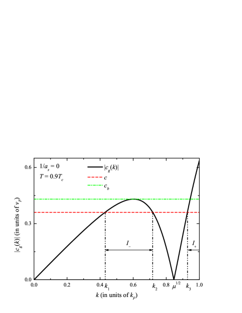
Figure 4: (Color online) Solid curve: the absolute value of the group velocity for the Bogoliubov excitations at $1/k_{F}a=0$ and $T=0.9T_{c}$. Dot-dashed line: the boundary velocity $c_{b}$ at the same parameters. Dashed line: an example of a value of $c$ at which the spectral function is computed. When $c<c_{b}$, the integration interval in the spectral function is made of two disconnected intervals whereas for $c>c_{b}$, it is made of a single interval.

Since $c_{g}(k)\rightarrow\infty$ when $k\rightarrow\infty$, the inequality $c<c_{g}\left(k\right)$ is always fulfilled for large enough $k>\sqrt{2m\mu}$. The interval $I_{+}(c)$ is then of the form $[k_{3}(c),+\infty[$. As visible in Fig. 4, the inequality $c<-c_{g}\left(k\right)$ can be also fulfilled at lower $k$ ($0<k<\sqrt{2m\mu}$) provided that $c$ is small enough, that is smaller than the boundary velocity,

$$c_{b}=\sqrt{\frac{{2\mu+3\Delta\left(\frac{1}{s^{1/3}}-s^{1/3}\right)}}{{m}}},\quad s\equiv\left(\mu/\Delta+\sqrt{\mu^{2}/\Delta^{2}+1}\right),$$ (72)

which is the absolute value of the minimum of the group velocity, $c_{b}=|\min_{k}\left[c_{g}\left(k\right)\right]|$ (in other words, the largest slope of the BCS branch $k\mapsto E_{k}$ in its decreasing part). The boundary sound velocity $c_{b}$ decreases when moving from the BCS to the BEC regime and vanishes when $\mu=0$, that is when the decreasing part of the BCS branch disappears. At a fixed scattering length, $c_{b}$ rises with increasing temperature because the chemical potential $\mu(T)$ rises. When the condition $c<c_{b}$ is fulfilled, the interval $I_{-}(c)$ exists and is of the form $[k_{1}(c),k_{2}(c)]$. Since $c_{g}(\sqrt{2m\mu})=0$, when the two momentum ranges exist they are disjoint ($k_{3}(c)>k_{2}(c)$). The boundary functions $k_{j}\left(c\right)$, $j=1,2,3$, when they exist, are the real positive roots of the polynomial equation,

$$\xi_{{k}}^{3}+\left(\mu-\frac{mc^{2}}{2}\right)\xi_{{k}}^{2}-\frac{mc^{2}}{2}\Delta^{2}=0,$$ (73)

with $\xi_{{k}}=k^{2}/2m-\mu$.

When $c\rightarrow c_{b}$ from below, the integral over $I_{-}$ in (70) tends to $0$, but its derivative can remain finite, which results in an angular point of the spectral function $\rho_{\sigma\sigma^{\prime}}$ in $c=c_{b}$. Physically, this angular point corresponds to the opening or closing of a decay channel in the decreasing part of the BCS branch, at $k<\sqrt{2m\mu}$. This angular point will become a branch point in the analytic continuation.

Choices for the analytic continuation

The spectral functions $\rho_{\sigma\sigma^{\prime}}\left(c\right)$ are analytic separately in the interval $A=[0,c_{b}[$ and $B=]c_{b},+\infty[$. Therefore there are two possible ways to continue them to $\operatorname{Im}(u)<0$:

$$\rho_{\sigma\sigma^{\prime}}^{(A)}(u) =u^{p}\left[\int_{k_{3}(u)}^{+\infty}dkf_{\sigma\sigma^{\prime}}(k,u)-\int_{k_{1}(u)}^{k_{2}(u)}dkf_{\sigma\sigma^{\prime}}(k,u)\right],$$ (74)

$$\rho_{\sigma\sigma^{\prime}}^{(B)}(u) =u^{p}\int_{k_{3}(u)}^{+\infty}dkf_{\sigma\sigma^{\prime}}(k,u),$$ (75)

where $k_{j}\left(u\right)$ for $j=1,2,3$, are the analytic continuations of the real solutions of (73). Numerically, these continuations are obtained by an adiabatic follow-up of the roots of (73) in the complex plane. Note that $k_{1}$ and $k_{2}$ can be continued to the entire half-plane with $\textrm{Im}\,u<0$ even though they are real only in the interval $[0,c_{b}]$ of the real axis. Choices (74) and (75) for the analytic continuation of the spectral functions translate into two possible analytic continuations $m_{\sigma\sigma^{\prime}}^{\left(A\right)}\left(u\right)$ and $m_{\sigma\sigma^{\prime}}^{\left(B\right)}\left(u\right)$. As shown in Fig. 5, when the analytic continuation is performed through the “window” $A$, a branch cut remains on interval $B$, and vice-versa.

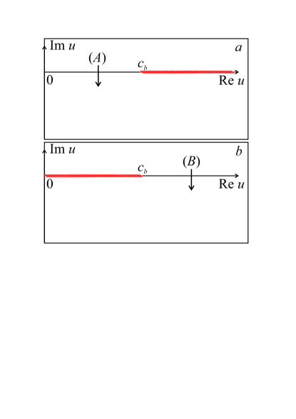
Figure 5: (Color online) Scheme of possible analytic continuations of coefficients $m_{\sigma\sigma^{\prime}}$ to the lower half-plane $\operatorname{Im}u<0$: through “window” $A$ (panel $a$), “window” $B$ (panel $b$). The branch cut of the analytically continued functions are shown by striped lines. The different analytic continuations have slightly different roots of the dispersion equation $W_{\downarrow}\left(u\right)=0$.

VI.2 Results and discussion

Using our “complex boundaries” numerical method to perform the analytic continuation, we study the solutions of the dispersion equation in the whole range $[0,T_{c}]$. The existence of two roots near $T_{c}$ is confirmed by our numerical study, a finding that does not depend on the choice of “window” $A$ or $B$ for the analytic continuation. In order to make the results quantitatively relevant for comparison with experiments, the sound velocity and damping are calculated here using the “scaled GPF” equation of state described in Appendix A.

BCS and around unitarity regimes

In the deep BCS regime, as shown in Fig. 6 the speed of Anderson-Bogoliubov first sound $c_{s,0}$ found at zero temperature evolves to the first root $u_{s,1}$ which we found near $T_{c}$. Both its real and imaginary part $c_{s,1}$ and $\kappa_{s,1}$ are monotonically increasing functions of temperature. The second solution $u_{s,2}$ appears only above a threshold temperature $T_{th}$, which tends to $T_{c}$ in the BCS limit. Its real part $c_{s,2}$ is zero at $T_{th}$ and at $T_{c}$ while its imaginary part $\kappa_{s,2}$ monotonically decreases with temperature. There is thus a regime in the range $[T_{th},T_{c}]$ where the two solutions are both well separated in frequency and comparable in damping. As visible in Fig. 7, the response function $\chi$ exhibits in this regime two distinguishable maxima (not just a peak with a shoulder as in Fig. 3) corresponding to the two roots of the analytic continuation. This unexpected finding is one of our key results; it validates the existence of two speeds of sound and thus of two collective modes in the GPF theory.

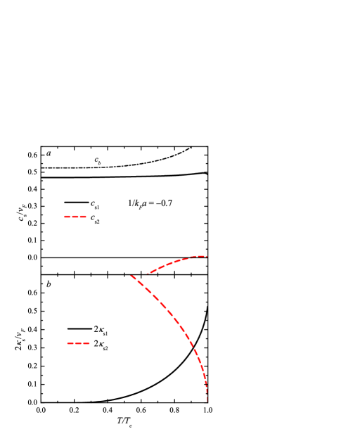
Figure 6: (Color online) The real (a) and imaginary parts $(b)$ of the two sound velocities $u_{\mathrm{s,1}}$ (black solid curves) and $u_{\mathrm{s,2}}$ (red dashed curves) in the BCS regime at $1/k_{F}a=-0.7$ (corresponding with the GPF equation of state to $\mu(T_{c})/T_{c}\simeq 6.06$ and $\left.\mu/\Delta\right|_{T=0}\simeq 3.34$) as functions of $T/T_{c}$. The dashed-dotted curve shows the boundary velocity $c_{b}$ (Eq. (72)) between sector $A$ (below $c_{b}$) and $B$ (above $c_{b}$) of the real axis.

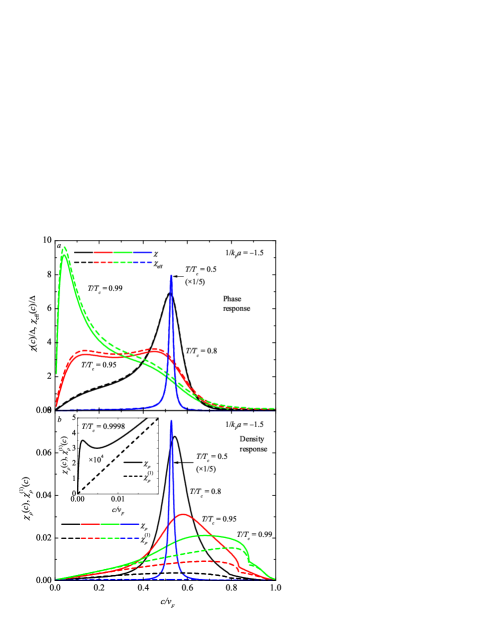
Figure 7: (Color online) Long-wavelength phase-phase response function $\chi\left(c\right)$ (solid lines) and its two-pole analytic approximation $\chi_{\mathrm{eff}}\left(c\right)$ (dashed lines) in the BCS regime ($1/k_{F}a=-1.5$, corresponding with the scaled GPF equation of state to $\left.\mu/\Delta\right|_{T=0}\simeq 12.1$) for $T=0.5T_{c}$ (blue lines), where they show a single quasi-Lorentzian peak, $T=0.8T_{c}$ (black lines), where the peak is displaced and skewed by the increasingly contributing second root, $T=0.95T_{c}$ where two resonances are visible (red lines) and $T=0.99T_{c}$ (green lines) where the low-velocity resonance found in Sec. V dominates. (b) Long-wavelength density-density response function $\chi_{\rho}\left(c\right)$ (solid curves) and the contribution of the pure density response $\chi_{\rho}^{\left(1\right)}\left(c\right)$ (dashed curves) for the same parameters of state as in the panel (a). Inset: Low-velocity part of the long-wavelength density-density response function in the close vicinity of the transition temperature, $T=0.9998T_{c}$.

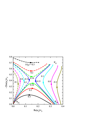
Figure 8: (Color online) The flow of the two roots of the dispersion equation (28) as a function of temperature, for different values of the inverse scattering length. The full curves show how the zero temperature root $c_{\mathrm{s}0}$ (lower right corner) evolves to either $u_{\mathrm{s}1}$ (upper right corner) or $u_{\mathrm{s}2}$ (lower left corner) as the temperature is increased up to $T_{c}$. The dashed curves show the temperature evolution of the other root, that appears in the upper left corner at the threshold temperature $T_{th}$. The labels near each curve show the corresponding value of $1/k_{F}a$ for this curve. The curves are obtained from the analytic continuation through window $A$, but the picture is qualitatively the same using window $B$.

At $1/k_{F}a=1/k_{F}a_{\mathrm{cross}}\simeq 0.155$ (corresponding with the GPF equation of state to $\mu(T_{c})/T_{c}\simeq 1.376$, hence still in the non-BEC regime of Sec. V), an exact crossing of the two roots occurs at a given temperature: $u_{\mathrm{s1}}(T_{\mathrm{cross}})=u_{\mathrm{s2}}(T_{\mathrm{cross}})$. Then, for $1/k_{F}a>1/k_{F}a_{\mathrm{cross}}$, the situation changes: the zero temperature solution $c_{s,0}$ evolves to $u_{s,2}$, while $u_{s,1}$ appears only above the threshold temperature $T_{th}$. As illustrated in Fig. 8, this behavior is reminiscent of that of two repulsive particles in $2D$, with temperature playing the role of time. The repulsion ensures that the trajectories never cross: if the $x$-coordinates (here $\textrm{Re}\,u$) cross, then the $y$-coordinates (here $\textrm{Im}\,u$) anticross, and vice-versa. In this analogy, the particular case $a=a_{\mathrm{cross}}$ corresponds to the infinite energy case where the two particles exactly meet.

BEC regime

As in Sec. V, we define the boundary of the BEC regime as the point where the chemical potential passes the zero value. Since $\mu$ depends on temperature, the condition $\mu(T)=0$ corresponds to different values of the interaction strength for different temperatures. In particular, with the GPF equation of state $\mu(T=0)=0$ results in $1/k_{F}a\approx 0.427$, and $\mu(T_{c})=0$ in $1/k_{F}a\approx 0.448$. The corresponding values of the inverse scattering length with the mean-field equation of state are, respectively, $1/k_{F}a\approx 0.553$ and $1/k_{F}a\approx 0.679$.

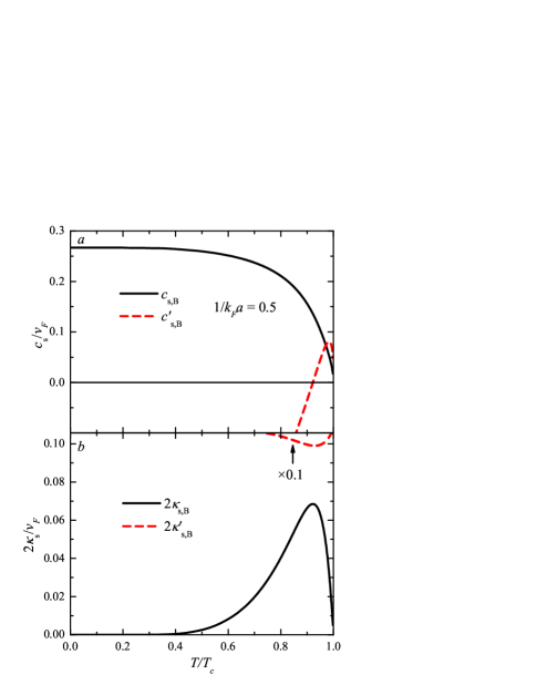
Figure 9: (Color online) The real (a) and imaginary parts (b) of the BEC regime sound velocity (black solid line) are shown at $1/k_{F}a=0.5$ (corresponding with the GPF equation of state to $\mu(T_{c})/T_{c}\simeq-0.293$ and $\left.\mu/\Delta\right|_{T=0}\simeq-0.139$) as functions of $T/T_{c}$. A second root (dashed red line) still exists in this regime but it is highly damped and thus irrelevant for the response function.

In the BEC regime, represented in Fig. 9, the $T=0$ solution $c_{s,0}$ always evolves to the solution $u_{s,B}$ that we found near $T_{c}$. Its real part $c_{s,B}$ decreases monotonically with temperature, while its imaginary part $\kappa_{\mathrm{s},B}$ vanishes at both $0$ and $T_{c}$, and goes through a maximum in between. The height of this maximum tends to zero in the BEC limit ($1/k_{F}a\to+\infty$), such that $\kappa_{\mathrm{s},B}(T)$ uniformly tends to zero in this limit. This is consistent with what we found in the vicinity of $T_{c}$ (Eq. (64)) and indicates that the damping mechanism we study (absorption-emission of collective excitations by fermionic quasiparticles) becomes less relevant in the BEC limit where the condensed pairs weakly interact with the unpaired fermions. As visible in Fig. 9, a second solution still exists in the BEC regime, but it is always largely damped such that it does not contribute to the response function, which never displays the two-peak behavior we described in the BCS regime.

Visibility of the phase collective modes in the density response

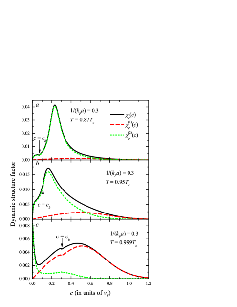
Figure 10: (Color online) Long-wavelength density response (Eq. (35)) function for $1/\left(k_{F}a\right)=0.3$ at (a) $T=0.87T_{c}$, (b) $T=0.95T_{c}$ and at (c) $T=0.999T_{c}$. Solid curves represent the total density response. Dashed and dotted curves show, respectively, contributions of pure density $\chi_{\rho}^{\left(1\right)}$ and order-parameter fluctuations $\chi_{\rho}^{\left(2\right)}$ to the total density response. The arrows indicate the boundary velocity $c_{b}$ determined by (72).

The two phase collective mode we have found are also visible in the density-density response function, as shown on Figs. 7 (b) and 10. At low temperature (blue curve in Fig. 7 (b)), the sole feature of $\chi_{\rho}\left(c\right)$ (which is uniformly dominated by the contribution $\chi_{\rho}^{(2)}$ of the pairing field) is the Anderson-Bogoliubov resonance. When the temperature rises, the Anderson-Bogoliubov resonance broadens and two other phenomena are visible: a broad incoherent peak due to the normal component $\chi_{\rho}^{(1)}$ appears at velocities $c$ of order $v_{F}$. This peak is not due to a collective mode (it does not have a Lorentzian shape) but simply to the density response of a normal Fermi gas which becomes increasingly dominant near $T_{c}$. At the same time, a resonance due to the $u_{s,2}$ pole of the pairing-field propagator forms at low-velocities, and becomes increasingly sharp when $T\to T_{c}$. The spectral weight of this resonance grows with increasing interaction strength (compare the inset of Fig. 7 (b) in the BCS limit to Fig. 10 (c) at strong coupling).

Note that in the density response we can clearly see the boundary velocity $c_{b}$ discussed above, which is related to the opening of a decay channel in the decreasing part of the BCS branch of excitations.

Influence of the choice of the analytic continuation

So far we have not discussed the physical consequences of having two windows $A$ ($0\leqslant c\leqslant c_{b}$) and $B$ ($c\geqslant c_{b}$) for the analytic continuation. For this, we go back to the physical observable, which are the response functions $\chi$ and $\chi_{\rho}$. Both of them have an angular point in $c_{b}$; this is an observable feature, not an artifact of the approximation we have used, nor of the collisionless regime. In fact, this angular point follows directly from energy conservation, and is caused by the non-monotonic nature of the quasiparticle spectrum which ensures that the low- and high-$k$ modes are separated by a point of zero group-velocity: the minimum of the BCS branch. Thus, this angular point is in a sense a signature of the superfluid phase. The physical meaning of the two windows $A$ and $B$ is then physically clear: window $A$ is appropriate to reproduce the low-velocity ($c<c_{b}$) part of the response functions and window $B$ for the high-velocity part ($c>c_{b}$).

When $c_{b}$ is far from the interesting features of the response function, that is from the resonance peaks centered around $c_{s,1}$ and $c_{s,2}$, then only one restriction of $\chi$, and thus only one analytic continuation, is worth studying. This is the case for example in the BCS limit: $c_{b}$ tends to $v_{F}$ which is well above both $c_{\mathrm{s},1}$ and $c_{\mathrm{s},2}$. The “window” $A$ (where the decay to quasiparticle of wave number $k<\sqrt{2m\mu}$ is allowed) is then the only choice. This reflects the fact that the BCS branch has a large decreasing part in this limit. Similarly, in the BEC regime, one has $c_{b}=0$, so that only the “window” $B$ is available for the analytic continuation.

On the contrary, when $c_{\mathrm{s}1}$ or $c_{\mathrm{s}2}$ cross $c_{b}$ at a given temperature (which occurs with the scaled GPF equation of state for $0.679\gtrapprox 1/k_{F}a\gtrapprox-0.594$; in Fig. 11 we show the example of unitary $1/|a|=0$), this means that the angular point in $c=c_{b}$ goes through the peak of $\chi$ as temperature varies, as illustrated in Fig. 12. Then, the roots found in window $A$ of the analytic continuation describe the left part of this broken peak, and those of window $B$, its right part. In practice, when they are close to $c_{b}$, the difference between the sound velocities $c_{\text{s}}^{\left(A\right)}$ and $c_{\text{s}}^{\left(B\right)}$ in the two windows is small with respect to their imaginary parts $\kappa_{\text{s}}$, as can be seen from Fig. 11. Physically, since the damping factor is a measure of the uncertainty of the sound velocity (following from the uncertainty relation between time and energy), this means that the difference in the velocity is almost indistinguishable, or in other words, that the discontinuity in the slope of the resonance peak can only be resolved through a very precise measurement of the response function.

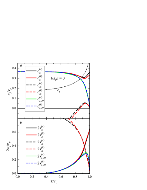
Figure 11: (Color online) The real (a) and imaginary parts $(b)$ of the two sound velocities $u_{\mathrm{s,1}}$ (black and red solid lines) and $u_{\mathrm{s,2}}$ (black and red dashed lines) are shown at unitarity $1/k_{F}a=0$ (corresponding to $\mu(T_{c})/T_{c}\simeq 1.50$ and $\left.\mu/\Delta\right|_{T=0}\simeq 0.86$) as functions of $T/T_{c}$. The dashed-dotted curve shows the boundary velocity $c_{b}$ (Eq. (72)) between sectors $A$ and $B$ of the real axis. In this regime, the resonance gets close to $c_{b}$, such that we should use window $A$ to describe the lower part ($0\leqslant c\leqslant c_{b}$) of the resonance ($u_{\mathrm{s,1}}^{(A)}$ and $u_{\mathrm{s,2}}^{(A)}$ are shown in black), and window $B$ for the upper part ($c_{b}\leqslant c$, $u_{\mathrm{s,1}}^{(B)}$ and $u_{\mathrm{s,2}}^{(B)}$ are shown in red). The green solid and blue dashed dotted lines show the effective sound velocities $u_{\mathrm{s,eff}}=c_{\mathrm{s,eff}}-i\kappa_{\mathrm{s,eff}}$ (defined in paragraph $d$ of Sec. VI.2) which characterize the position and width of the peak in the response function $\chi$, which is always unique at unitarity.

Analytic approximation for the response function

From the poles $u_{\textrm{s},1}$ and $u_{\textrm{s},2}$ found in the analytic continuation, and their residues $Z_{1}$ and $Z_{2}$ in the phase-phase propagator $\textrm{Im}\,m_{--}/\pi W$ one can construct an effective response function, in the BCS regime:

$$\chi_{\mathrm{eff}}\left(c\right)=\begin{cases}\frac{1}{\pi}\operatorname{Im}\left(\frac{Z_{1}^{(A)}}{c-u_{\mathrm{s1}}^{(A)}}+\frac{Z_{2}^{(A)}}{c-u_{\mathrm{s2}}^{(A)}}\right)\quad\textrm{if}\quad 0\leqslant c\leqslant c_{b}\\ \frac{1}{\pi}\operatorname{Im}\left(\frac{Z_{1}^{(B)}}{c-u_{\mathrm{s1}}^{(B)}}+\frac{Z_{2}^{(B)}}{c-u_{\mathrm{s2}}^{(B)}}\right)\quad\textrm{if}\quad c\geqslant c_{b},\end{cases}$$ (76)

which is the sum of the two resonance peaks caused by $u_{\textrm{s},1}$ and $u_{\textrm{s},2}$ in each window $A$ and $B$. Note that since the residues $Z_{1}$ and $Z_{2}$ are complex, this is not simply the sum of two Lorentzian functions. Conversely, in the BEC regime, our effective response function has only one resonance

$$\chi_{\mathrm{eff,B}}\left(c\right)=\frac{1}{\pi}\operatorname{Im}\left(\frac{Z_{\rm B}}{c-u_{\mathrm{s,B}}}\right)$$ (77)

These functions can be compared with the exact response function $\chi$, to check the relevance of the analytic structure found in the analytic continuation. They allow to interpret the shape of $\chi$ in terms of resonances caused by collective modes. They can also be used as fitting functions for experimentalists to extract the values of $u_{\textrm{s},1}$, $u_{\textrm{s},2}$ or $u_{\textrm{s,B}}$ and their residues from a measured response spectrum.

In the low-temperature case (see the example of $T=0.4T_{c}$ in the inset $(a)$ of Fig. 12) the residue of the only relevant complex root tends to a real number, such that we expect the response function $\chi$ to have an approximate Lorentzian shape. This is indeed what we observe in Fig. 12, with a very good agreement between $\chi$ and $\chi_{\mathrm{eff}}$. When raising the temperature, away from the BCS regime one does not immediately observe the formation of a second peak (see the examples of $T=0.87T_{c}$ and $T=0.95T_{c}$ in Fig.  12), but rather a shift in the position of the original peak and an increase of its width and skewness. To describe the altered peak, we introduce an effective sound velocity $u_{\mathrm{s,eff}}=c_{\mathrm{s,eff}}-i\kappa_{\mathrm{s,eff}}$ where $c_{\mathrm{s,eff}}$ is the value of $c$ where $\chi_{\mathrm{eff}}$ reaches its maximum, and $\kappa_{\mathrm{s,eff}}$ its half width at half maximum. These quantities are useful only close to $T=0$ and $T_{c}$ where one root is much less damped than the other. In the intermediate temperature regime where the two roots have a comparable damping rate, the response function is not well fitted by a single Lorentzian, and one should revert to the superposition introduced in (76). This particularly the case in the far BCS regime where the response function exhibits two distinct peaks in a temperature range close to but excluding $T_{c}$ (see the example of $T=0.95T_{c}$ in Fig. 7).

As we said above, at and around unitarity, the angular point in $c_{b}$ goes through the resonance peak as temperature varies. This results in a visibly broken peak in $\chi$, which is again well captured by our two-pole analytic approximation $\chi_{\rm eff}$ provided one switches of the interval of analytic continuation when crossing $c_{b}$, as prescribed by Eq. (76). When the argument $c=\omega/q$ of the response function passes the boundary velocity $c_{b}$, $\chi\left(c\right)$ exhibits an angular point and its two-pole analytic approximation $\chi_{\mathrm{eff}}\left(c\right)$ exhibits a discontinuity.

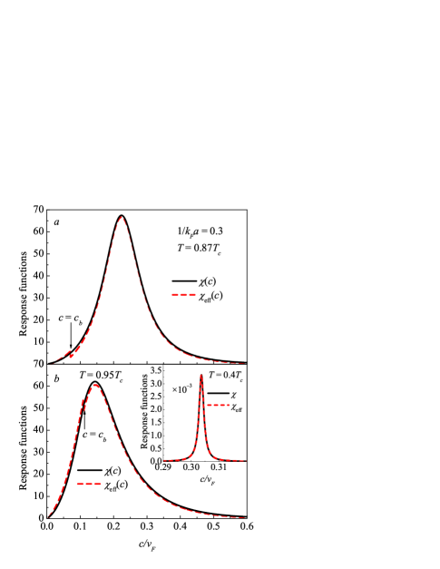
Figure 12: (Color online) Long-wavelength phase-phase response function $\chi\left(c\right)$ and its two-pole analytic approximation $\chi_{\mathrm{eff}}\left(c\right)$ at $1/k_{F}a=0.3$). At $T=0.4T_{c}$ (inset), both show a single quasi-Lorentzian peak. At $T=0.87T_{c}$ (panel $a$), the boundary velocity $c_{b}$, which is an angular point for $\chi$ and a discontinuity for $\chi_{\mathrm{eff}}$, lies below the maximum of the resonance. At $T=0.95T_{c}$ (panel $b$) the angular point shifts towards higher $c$.

VII Links to other theories and to experiments

VII.1 Comparison to low temperature approaches

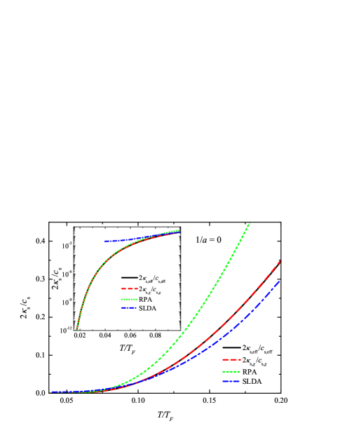
Figure 13: (Color online) Long-wavelength inverse quality factor of the Bogoliubov-Anderson mode at unitarity and at low temperature. Solid curve: An effective quality factor is computed from the poles $u_{s1}$ and $u_{s2}$ in the analytic continuation by taking into account the unicity of the resonance at low temperature (see Eqs. (78) and (79)). Dashed curve: The quality factor is extracted directly from the long-wavelength response function $\chi\left(c\right)$. In both cases we use the equation of state obtained within the GPF approximation HLD , instead of the mean-field one. Dotted curve: the RPA low-temperature asymptotic behavior according to Kurkjian2017-2 is recalculated using the GPF equation of state. Dotted curve: the SLDA result of Ref. Zou . Inset: the same in a lower temperature range, in the logarithmic scale.

In Fig. 13, we plot the inverse quality factor $2\kappa_{\mathrm{s,eff}}/c_{\mathrm{s,eff}}$ of the phononic modes as a function of the temperature at unitarity where we use the scaled GPF equation of state. In this regime, our result can be compared to several other approaches (which all assumed the existence of a unique phononic mode, hence our use of the effective velocity). (i) A prediction based on Landau phonon-roton theory (which is exact if the roton branch is known exactly, see Eqs. (15-16) of Kurkjian2017-3 ; it is recalculated here using the BCS branch as the roton branch and the GPF parameters of state) exactly agrees with our asymptotic results when $T\rightarrow 0$. (ii) The superfluid local density approximation (SLDA) Zou , an approach which exploits the universal behavior of the gas at unitarity, also predicts a quality factor due to the coupling to the fermionic quasiparticle-quasihole continuum in good quantitative agreement with ours except the low-temperature range where the damping rate obtained in Zou seems aberrant as it does not tend to zero when $T\rightarrow 0$.

VII.2 Comparison to measurements of the sound velocity

In Fig. 14, the nonzero-temperature effective sound velocity $c_{\mathrm{s,eff}}$ as a function of $1/k_{F}a$ calculated within the present approach is compared with the experimental data of Ref. Hoinka (squares) using different equations of state. Since the experimental value of the speed of sound were obtained using a single Gaussian fit of the response function, it is natural to compare them to our effective sound velocity (which combines the information about the two resonances in a unique velocity).

The temperatures throughout the BCS-BEC crossover are determined by a quadratic interpolation of the experimental values reported in Ref. Hoinka : $k_{B}T=0.09E_{F}$ at unitarity, $k_{B}T=0.02E_{F}$ at $1/k_{F}a=-1.6$, and $k_{B}T=0.1E_{F}$ at $1/k_{F}a=1$ (such that $T/T_{c}$ is about $1/2$ in all three cases). The sound velocity has been calculated here using our results for $c_{s}(\Delta/\mu,\Delta/T)$, and the mean-field gap equation with the chemical potential obtained by three methods: (1) from the Table 3 of the Supplement to Ref. Hoinka , (2) from the number equation accounting for Gaussian pair fluctuations within the NSR scheme for the superfluid state below $T_{c}$ Engelbrecht , and (3) from the GPF approach of Refs. Diener2008 ; HLD ; HLD1 (almost equivalent to the scaled GPF equation of state of Appendix A since the temperature is lower than $T_{c}$ here). As can be seen from Fig. 14, an excellent agreement with the experiment is obtained when we use the parameters of state from Ref. Hoinka .

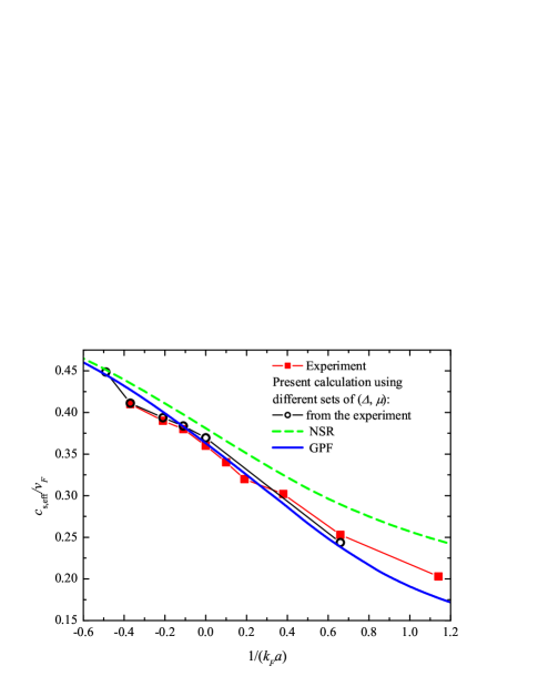
Figure 14: (Color online) Nonzero-temperature sound velocity $c_{\mathrm{s}}$ as a function of $1/k_{F}a$ calculated within the present approach using different sets of background parameters $\left(\mu,\Delta\right)$: with background parameters extracted from Hoinka (empty dots), with parameters calculated accounting for Gaussian fluctuations within the NSR scheme for the superfluid (broken-symmetry) state Engelbrecht (dashed curve) and within the GPF scheme of Refs. Diener2008 ; HLD ; HLD1 (solid curve). The calculated sound velocities are compared with the experimental data of Ref. Hoinka (squares).

VII.3 Measuring the phase-phase response

So far the experiments have measured the collective mode spectrum through the density response of the gas. It would be interesting to access also the phase-phase response function, particularly near $T_{c}$ where it has a very different shape than the density-density response as we have seen. To this end, we explain how one can adapt the Carlson-Goldman Goldman1976 experiment, which measured the pairing-field susceptibility of a superconductor, to a cold atom setup. The scheme we propose is illustrated on Fig. 15, and it uses only existing experimental techniques.

Figure 15: Experimental setup designed to measure the phase-phase response function $\chi$ of a superfluid Fermi gas at $T\lessapprox T_{c}$ (left well). A spatially dependent tunneling barrier (in the middle) couples the system to a reservoir (right well) consisting of a fully paired Fermi gas at $T=0$. This creates a spatially dependent excitation of the phase of the order parameter in the left well. This phase pattern is measured at the end of the experimental sequence by letting the gases in the left and right wells expand and interfere.

The excitation is obtained by coupling the system of interest (a superfluid Fermi gas at nonzero temperature, for example at $T$ close to $T_{c}$) to a environment consisting of a large superfluid Fermi gas prepared at zero temperature and with a well-defined phase with respect to the system (which can be done by initially performing Josephson oscillations Roati2015 ). The two gases are coupled through a tunneling barrier, similar to the thin barrier realized in Roati2015 ; to extract information on the spectrum at momentum $q$, the barrier should be spatially modulated at a wavelength $\lambda=2\pi/q$, which, for instance, could be achieved by interfering two laser fields. The fact that the reservoir gas is much larger than the studied system ensures that it remains at zero temperature all along the excitation time, and that its quantum fluctuations can be neglected. It behaves then as a classical pairing field imposed on the system, which can be represented by the drive term in the Hamiltonian

$$\hat{H}_{\rm drive}(t)=\int d^{3}rJ(\textbf{r},t)\Delta_{\rm exc}^{*}\hat{\psi}_{\downarrow}(\textbf{r},t)\hat{\psi}_{\uparrow}(\textbf{r},t)+\mbox{h.c.}$$ (81)

Here $\Delta_{\rm exc}$ is the order parameter of the reservoir (whose phase has been fixed initially) and $J(\textbf{r},t)=J(t)\times\cos(qy)$ is the spatially dependent strength of the barrier; since the system is prepared close to $T_{c}$, its healing length is very large, and we can assume the effect of the barrier to be homogeneous in the $x$-direction Goldman1976 . The time-dependence of $J$ can be either sinusoidal $J(t)\propto\cos(\omega t+\phi)$ if one wishes to probe the response function at a given frequency $\omega$, or it can be more abrupt if one wishes to study the quench-like dynamics of the system (which theoretically is described by the Laplace transform of the frequency-domain response function $\chi$ Gurarie2009 ). Finally, the phase of the system is measured by letting the cloud expand and interfere with the reservoir as in Roati2015 . The interference pattern will appear shifted in the $x$ direction by a length $\delta x(y)$ which depends on the local phase of the system at position $y$.

VIII Conclusions

We have studied the long-wavelength solutions to the RPA/GPF equation on the collective mode energy of a neutral fermionic condensate. To access the full range of temperatures between zero and $T_{c}$, we deal non-perturbatively with the damping caused by absorption/emission of BCS “broken-pair” quasiparticles. For that, we set the energy proportional to the wave vector, $z=uq$, and analytically continue the equation for $u$ through its branch cut associated to the quasiparticle absorption-emission continuum.

While our results at low temperature agree with previous perturbative approaches in predicting a single collective mode with an exponentially small damping rate and velocity shift, we find an unexpected second solution in the vicinity of the transition temperature $T_{c}$. This two-mode nature is also visible in the order-parameter phase response function which displays two distinct resonance peaks, at temperatures relatively close to $T_{c}$, and in the BCS regime. In the limit $T\to T_{c}$, we show analytically that the velocity of the first mode tends to a finite and non-zero complex number, while the damping rate of the second mode vanishes like $\Delta(T)$ (or $(T_{c}-T)^{1/2}$), and its quality factor vanishes logarithmically. In the BEC regime, on the contrary, we find only one relevant solution, whose velocity vanishes like $(T_{c}-T)^{1/2}$ near $T_{c}$ with a diverging quality factor.

At arbitrary temperatures $0<T<T_{c}$, we develop a numerical method to perform the analytic continuation of the GPF equation. This confirms the existence of two distinct phononic branches, one being dominant near $T=0$, the other near $T_{c}$. The transition between these two resonances is visible in both the phase-phase and density-density response functions. Last, our knowledge of the two poles in the analytic continuation, and of their residues, allows us to propose an analytic function to describe the phase response in terms of two collective resonances.

The present study not only resolves some problems but also raises new questions, particularly about the existence, outside the collisionless regime, of the transition we have seen between two distinct collective modes. This transition undoubtedly exists in the GPF approximation, but a more systematic treatment should account for the finite lifetime of the fermionic quasiparticles Zwerger2009 . In any case, our work will be heuristically useful for further developments of the theory of collective excitations in superfluid Fermi gases.

Appendix A Equation of state accounting for order-parameter fluctuations

The next-order approximation beyond mean-field is used to account for fluctuations of the pair field about the saddle-point solution. This comes from the expansion of the effective bosonic action in powers of the fluctuation coordinates up to the second order. The resulting thermodynamic potential is a sum of the saddle-point and fluctuation contributions:

$$\Omega=\Omega_{\rm sp}+\Omega_{\rm fluct},$$ (82)

with the saddle-point and fluctuation contributions:

$$\Omega_{\rm sp} =-\int\frac{d^{3}k}{\left(2\pi\right)^{3}}\left[\frac{1}{\beta}\ln\left(2+2\cosh\beta E_{\mathbf{k}}\right)-\xi_{\mathbf{k}}-\frac{m\Delta^{2}}{k^{2}}\right]-\frac{m\Delta^{2}}{4\pi a},$$ (83a)

$$\Omega_{\rm fluct} =\frac{1}{2\beta}\sum_{\mathbf{q},n}\ln\det\mathbb{M}\left(\mathbf{q},i\Omega_{n}\right),$$ (83b)

where the matrix elements of the inverse Gaussian pair fluctuation $$M\left(\mathbf{q},i\Omega_{n}\right)$$ propagator are described above.

Within the Nozières – Schmitt-Rink (NSR) scheme deMelo1993 extended to the superfluid state below $T_{c}$ in Ref. Engelbrecht (see also Ohashi2006 ; PRA2008 ), the particle density is determined as

$$n=-\left.\left(\frac{\partial\Omega}{\partial\mu}\right)\right|_{T,\Delta}$$ (84)

considering $\Delta$ as an independent parameter. The NSR scheme has been modified Diener2008 ; HLD taking into account a variation of the gap:

$$n=-\left.\left(\frac{\partial\Omega}{\partial\mu}\right)\right|_{T,\Delta}-\left.\left(\frac{\partial\Omega}{\partial\Delta}\right)\right|_{T,\mu}\left.\left(\frac{\partial\Delta}{\partial\mu}\right)\right|_{T}.$$ (85)

This approximation, referred to as GPF (Gaussian Pair Fluctuation approximation) provides the temperature dependence of the chemical potential in good agreement with Quantum Monte Carlo results Astr ; Bulgac2006 .

The parameters of state accounting for fluctuations are related to the saddle-point parameters of state through the exact scaling relations

$$\Delta\left(\frac{1}{a},T,\mu\right)=\Delta_{sp}\left(\frac{1}{a_{sp}},T_{sp},\mu_{sp}\right)\frac{E_{F}^{\left(sp\right)}\left(\frac{1}{a_{sp}},T_{sp},\mu_{sp}\right)}{E_{F}\left(\frac{1}{a_{sp}},T_{sp},\mu_{sp}\right)}$$ (86)

where $\left(\frac{1}{a_{\rm sp}},T_{\rm sp},\mu_{\rm sp}\right)$ are related to the true $\left(\frac{1}{a},T,\mu\right)$ by the equations:

$$\frac{a}{a_{\rm sp}} =\sqrt{\frac{E_{F}\left(\frac{1}{a_{\rm sp}},T_{\rm sp}\right)}{E_{F}^{\rm\left(sp\right)}\left(\frac{1}{a_{\rm sp}},T_{\rm sp}\right)}},$$ (87)

$$\frac{T}{T_{\rm sp}} =\frac{\mu}{\mu_{\rm sp}}=\frac{E_{F}^{\rm\left(sp\right)}\left(\frac{1}{a_{\rm sp}},T_{\rm sp}\right)}{E_{F}\left(\frac{1}{a_{\rm sp}},T_{\rm sp}\right)},$$ (88)

with the Fermi energies $E_{F}$ and $E_{F}^{\left(sp\right)}$ calculated, respectively, with and without accounting for fluctuations:

$$E_{F}=\frac{\hbar^{2}\left(3\pi^{2}n\right)^{2/3}}{2m},\quad E_{F}^{\left(sp\right)}=\frac{\hbar^{2}\left(3\pi^{2}n_{sp}\right)^{2/3}}{2m}.$$ (89)

These scaling relations precisely reproduce the GPF or NSR schemes [depending of a choice for $n$, (84) or (85)]. Close to the transition temperature, both NSR and GPF schemes reveal an artifact: a discontinuous change of the gap from a finite value to zero at $T_{c}$. In order to overcome this issue and study sound velocities in a superfluid Fermi gas for all $T<T_{c}$, several interpolation schemes were considered in Refs. Taylor2008 ; Taylor . In the present work, we use a slightly different interpolation scheme. The chemical potential calculated within the GPF approach HLD ; HLD1 shows an excellent agreement with the Monte Carlo results for $T<T_{c}$ Bulgac2006 , where the transition temperature $T_{c}$ is determined accounting for fluctuations and is the same within the GPF and NSR schemes HLD1 . Moreover, both the chemical potential and the gap calculated within GPF at $T=0$ are in good agreement with these Monte Carlo calculations. Therefore we keep the relations (87) and (88) unchanged, so that the chemical potential remains the same as within GPF, and replace (86) by the equation:

$$\Delta\left(\frac{1}{a},T,\mu\right)=\Delta_{sp}\left(\frac{1}{a_{sp}},T_{sp}^{\prime},\mu_{sp}\right)\frac{E_{F}^{\left(sp\right)}\left(\frac{1}{a_{sp}},T_{sp},\mu_{sp}\right)}{E_{F}\left(\frac{1}{a_{sp}},T_{sp},\mu_{sp}\right)},$$ (90)

where $T_{\rm sp}$ in the temperature dependence of $\Delta_{\rm sp}$ is rescaled as $T_{\rm sp}^{\prime}\equiv\left(T_{c}^{\rm\left(sp\right)}/T_{c}\right)T$. According to (90), the gap takes the value $\Delta=\Delta_{\rm GPF}$ at $T=0$, and tends to zero as $\Delta\propto\sqrt{T_{c}-T}$ when approaching $T_{c}$. This known behavior of $\Delta$ in the vicinity of $T_{c}$ is an exact universal condition, independent on the coupling strength. Eq. (90) is thus a renormalized saddle-point gap equation in which the aforesaid artifacts of the temperature dependence of $\Delta\left(T\right)$ are removed.

Appendix B Details of the calculation near $T_{c}$

In this Appendix, we detail the calculation of the integrals in Eqs. (23–25) in the limit $T\to T_{c}$. We recall the notations of Sec. V: $\epsilon=\Delta/T$ is our small parameter, $\mu/T=m_{c}+O(\epsilon^{2})$, and $\mu/\Delta=m_{c}/\epsilon+O(\epsilon)$. We first replace the tridimensional integral in the following way

$$\int\frac{d^{3}k}{(2\pi)^{3}}\to\frac{\rho(\mu)\Delta}{2}\int_{-m_{c}/\epsilon}^{\infty}\check{k}(\xi)d\xi\int_{0}^{1}dt$$ (91)

where $\rho(\mu)=\sqrt{2m^{3}\mu}/\pi^{2}\hbar^{3}$ is the density of states at energy $\mu$ (setting the gas volume equal to $1$), $t=\cos\theta$, $\xi=\xi_{k}/\Delta$, $\check{k}^{2}=k^{2}/2m\mu=1+\epsilon\xi/m_{c}+O(\epsilon^{3})$ and we use later $E^{2}=\xi^{2}+1$.

BCS regime

In the BCS regime ($m_{c}>0$), we give the formulary of $\epsilon$-expanded integrals:

$$\int_{-m_{c}/\epsilon}^{\infty}d\xi\frac{\check{k}^{p}(\xi)\textrm{tanh}(\epsilon E/2)}{E^{3}} = \epsilon\frac{\pi}{2}+\epsilon^{2}f_{p}(m_{c})+O(\epsilon^{3}),\qquad p=1,3$$ (92)

$$\int_{-m_{c}/\epsilon}^{\infty}d\xi\frac{\check{k}^{p}(\xi)\textrm{tanh}^{\prime}(\epsilon E/2)}{E^{2}} = {\pi}+\epsilon g_{p}(m_{c})O(\epsilon^{2}),\qquad p=1,3$$ (93)

$$\int_{-m_{c}/\epsilon}^{\infty}d\xi\frac{\check{k}(\xi)\textrm{tanh}(\epsilon E/2)}{E^{3}}\xi = \epsilon h_{1}(m_{c})+O(\epsilon^{3})$$ (94)

The leading orders are obtained by simply expanding the integrand at low $\epsilon$: ${\check{k}^{p}(\xi)\textrm{tanh}(\epsilon E/2)}/{E^{n}}=\epsilon/{2E^{n-1}}+O(\epsilon^{2})$, and ${\check{k}^{p}(\xi)\textrm{tanh}^{\prime}(\epsilon E/2)}/{E^{n}}=1/{E^{n}}+O(\epsilon^{2})$ which gives rise to converging integrals. To compute the subleading term, we add and subtract the leading one to ensure the convergence of the $\epsilon$-expanded integral in $\xi=0$, perform the change of variable $e=\epsilon\xi$, and approximate $\epsilon E\simeq e$. We get

$$f_{p}(m_{c})=-\frac{1}{m_{c}}+\int_{0}^{m_{c}}de\left\{\frac{\textrm{tanh}(e/2)}{e^{3}}\left[\left(1+\frac{e}{m_{c}}\right)^{p/2}+\left(1-\frac{e}{m_{c}}\right)^{p/2}\right]-\frac{1}{e^{2}}\right\}\\ +\int_{m_{c}}^{\infty}de\frac{\textrm{tanh}(e/2)}{e^{3}}\left(1+\frac{e}{m_{c}}\right)^{p/2}\qquad p=1,3$$ (95)

$$g_{p}(m_{c})=-\frac{2}{m_{c}}+\int_{0}^{m_{c}}de\left\{\frac{\textrm{tanh}^{\prime}(e/2)}{e^{2}}\left[\left(1+\frac{e}{m_{c}}\right)^{p/2}+\left(1-\frac{e}{m_{c}}\right)^{p/2}\right]-\frac{2}{e^{2}}\right\}\\ +\int_{m_{c}}^{\infty}de\frac{\textrm{tanh}^{\prime}(e/2)}{e^{2}}\left(1+\frac{e}{m_{c}}\right)^{p/2}\qquad p=1,3$$ (96)

$$h_{1}(m_{c})=\int_{0}^{m_{c}}de\frac{\textrm{tanh}(e/2)}{e^{2}}\left[\left(1+\frac{e}{m_{c}}\right)^{1/2}-\left(1-\frac{e}{m_{c}}\right)^{1/2}\right]+\int_{m_{c}}^{\infty}de\frac{\textrm{tanh}(e/2)}{e^{2}}\left(1+\frac{e}{m_{c}}\right)^{1/2}$$ (97)

In $m_{++}$, $m_{--}$, $m_{+-}$, the integrals with a resonant denominator give

$$\int_{-m_{c}/\epsilon}^{\infty}d\xi\int_{0}^{1}dt\frac{\check{k}^{3}t^{2}\textrm{tanh}^{\prime}\left({\epsilon E}/{2}\right)}{E^{2}(E^{2}\check{u}^{2}-t^{2}\xi^{2}\check{k}^{2})} = \pi+4F(\check{u})+O(\epsilon^{2})$$ (98)

$$\int_{-m_{c}/\epsilon}^{\infty}d\xi\int_{0}^{1}dt\frac{\check{k}^{3}t^{2}\textrm{tanh}^{\prime}\left({\epsilon E}/{2}\right)\xi^{2}}{E^{2}(E^{2}\check{u}^{2}-t^{2}\xi^{2}\check{k}^{2})} = -\pi+4G(\check{u})-\epsilon G_{2}(\check{u},m_{c})+O(\epsilon^{2})$$ (99)

$$\int_{-m_{c}/\epsilon}^{\infty}d\xi\int_{0}^{1}dt\frac{\check{k}^{3}t^{2}\textrm{tanh}^{\prime}\left({\epsilon E}/{2}\right)\xi}{E^{2}(E^{2}\check{u}^{2}-t^{2}\xi^{2}\check{k}^{2})} = \epsilon H(\check{u},m_{c})+O(\epsilon^{2})$$ (100)

The functions $F$ and $G$ are given in the main text [Eqs. (45)-(46)]. Functions $G_{2}$ and $H$ characterizing the subleading order terms to $m_{--}$ and $m_{+-}$ can be written in integral forms similar to Eqs. (95–97), which we don’t give explicitly. In fact, we will need only the value of these functions in $\check{u}$=0:

$$G_{2}(0,m_{c}) = g_{1}(m_{c})$$ (101)

$$H(0,m_{c}) = 0$$ (102)

Combining our two formularies (92–94) and (98–100), to the definition of $m_{\sigma\sigma^{\prime}}$ (Eqs. (23–25)), we obtain equations (42–44) of the main text, with

$$f = \frac{f_{3}}{6}-\frac{g_{3}}{12}$$ (103)

$$g = \frac{f_{1}}{2}-\frac{g_{1}}{4}$$ (104)

$$h = -\frac{h_{1}}{4}$$ (105)

BEC regime

In the BEC regime ($m_{c}<0$), the integral over $\xi$ in (91) begins from $|{m_{c}}|/\epsilon\gg 1$. To leading order, one then approximates $E\simeq\xi$, and performs the change of variable $e=\epsilon\xi$. We give the new formulary of integrals

$$\int_{|m_{c}|/\epsilon}^{\infty}d\xi\frac{\check{k}^{p}(\xi)\textrm{tanh}(\epsilon E/2)}{E^{3}} = \epsilon^{2}f_{p}^{\rm B}(m_{c})+O(\epsilon^{4}),\qquad p=1,3$$ (106)

$$\int_{|m_{c}|/\epsilon}^{\infty}d\xi\frac{\check{k}^{p}(\xi)\textrm{tanh}^{\prime}(\epsilon E/2)}{E^{2}} = \epsilon g_{p}^{\rm B}(m_{c})+O(\epsilon^{3}),\qquad p=1,3$$ (107)

$$\int_{|\mu|/\Delta}^{\infty}d\xi\frac{\check{k}(\xi)\textrm{tanh}(\epsilon E/2)}{E^{3}}\xi = \epsilon h_{1}^{\rm B}(m_{c})+\epsilon^{3}h_{3}^{\rm B}(m_{c})+O(\epsilon^{4})$$ (108)

$$\int_{|m_{c}|/\epsilon}^{\infty}d\xi\int_{0}^{1}dt\frac{\check{k}^{3}t^{2}\textrm{tanh}^{\prime}\left({\epsilon E}/{2}\right)}{E^{2}(E^{2}\check{u}^{2}-t^{2}\xi^{2}\check{k}^{2})} = O(\epsilon^{3})$$ (109)

$$\int_{|m_{c}|/\epsilon}^{\infty}d\xi\int_{0}^{1}dt\frac{\check{k}^{3}t^{2}\textrm{tanh}^{\prime}\left({\epsilon E}/{2}\right)\xi^{2}}{E^{2}(E^{2}\check{u}^{2}-t^{2}\xi^{2}\check{k}^{2})} = \epsilon\left[-g_{1}^{\rm B}(m_{c})+4\check{u}B(\check{u},m_{c})\right]+O(\epsilon^{2})$$ (110)

$$\int_{|\mu|/\Delta}^{\infty}d\xi\int_{0}^{1}dt\frac{\check{k}^{3}t^{2}\textrm{tanh}^{\prime}\left({\epsilon E}/{2}\right)\xi}{E^{2}(E^{2}\check{u}^{2}-t^{2}\xi^{2}\check{k}^{2})} = \epsilon^{2}C_{2}(\check{u},m_{c})+O(\epsilon^{3})$$ (111)

The integrals containing a resonant denominator are obtained after the decomposition

$$\frac{\check{k}^{3}t^{2}\textrm{tanh}^{\prime}\left({\epsilon E}/{2}\right)}{E^{2}(E^{2}\check{u}^{2}-t^{2}\xi^{2}\check{k}^{2})}=-\frac{\check{k}\textrm{tanh}^{\prime}\left({\epsilon E}/{2}\right)}{\xi^{2}E^{2}}+\frac{\check{u}\check{k}\textrm{tanh}^{\prime}\left({\epsilon E}/{2}\right)}{2\xi^{2}E}\left(\frac{1}{E\check{u}-t\xi\check{k}}+\frac{1}{E\check{u}+t\xi\check{k}}\right)$$

Using this formulary, we obtain equations (55–57) of the main text, with

$$\alpha_{1}(m_{c}) = |m_{c}|\left(\frac{f_{3}^{\rm B}(m_{c})}{6}-\frac{g_{3}^{\rm B}(m_{c})}{12}\right)$$ (112)

$$\alpha_{2}(m_{c}) = -\frac{|m_{c}|\,f_{1}^{\rm B}(m_{c})}{2}$$ (113)

$$\beta(m_{c}) = \frac{f_{1}^{\rm B}(m_{c})}{2}-\frac{g_{1}^{\rm B}(m_{c})}{4}$$ (114)

$$\gamma(m_{c}) = -\frac{h_{1}^{\rm B}(m_{c})}{4}$$ (115)

$$C(\check{u},m_{c}) = -\frac{h_{3}^{\rm B}(m_{c})}{4}+\frac{C_{2}(\check{u},m_{c})}{8}$$ (116)

Appendix C Dynamic structure factor

The density-density response function is determined here within the Random Phase Approximation, similarly to Refs. Minguzzi et al. (2001); Zou2010 and the BCS-Leggett response theory of Ref. He2016 . The real-time density-density response is described by the retarded Green’s function

$$G_{\rho}^{R}\left(\mathbf{q},\omega+i0^{+}\right)\equiv-i\lim_{\delta\rightarrow+0}\int_{0}^{\infty}e^{i\omega t-\delta t}\int d\mathbf{r}\leavevmode\nobreak\ e^{-i\mathbf{q}\cdot\mathbf{r}}\left\langle\left[\rho\left(\mathbf{r},t\right),\rho\left(0,0\right)\right]\right\rangle dt,$$ (117)

where $\rho\left(\mathbf{r},t\right)$ is the particle density:

$$\rho\left(\mathbf{r},t\right)=\bar{\psi}_{\mathbf{r},t,\uparrow}\psi_{\mathbf{r},t,\uparrow}+\bar{\psi}_{\mathbf{r},t,\downarrow}\psi_{\mathbf{r},t,\downarrow}.$$ (118)

The spectral weight function (the dynamic structure factor) is proportional to the imaginary part of $G_{\rho}^{R}$:

$$\chi_{\rho}\left(\mathbf{q},\omega\right)=-\frac{1}{\pi}\operatorname{Im}G_{\rho}^{R}\left(\mathbf{q},\omega+i0^{+}\right).$$ (119)

We use the known correspondence between the Green’s function in the Matsubara representation $\mathcal{G}_{\rho}\left(\mathbf{q},i\Omega_{m}\right)$ and the retarded two-point Green’s function $G_{\rho}^{R}\left(\mathbf{q},\omega+i0^{+}\right)$ [e. g., Mahan , Eq. (3.3.11)]:

$$G_{\rho}^{R}\left(\mathbf{q},\omega+i0^{+}\right)=\leavevmode\nobreak\ \underset{i\Omega_{m}\rightarrow\omega+i0^{+}}{\mathcal{G}_{\rho}\left(\mathbf{q},i\Omega_{m}\right).}$$ (120)

The Green’s function in the Matsubara representation $\mathcal{G}_{\rho}\left(\mathbf{q},i\Omega_{m}\right)$ is determined using the generating functional in the path-integral representation with the auxiliary infinitesimal field variable $\upsilon\left(\mathbf{r},\tau\right)$ corresponding to density fluctuations,

$$\Xi\left(\upsilon\right)=\left\langle\exp\left[\int_{0}^{\beta}d\tau\int d\mathbf{r}\leavevmode\nobreak\ \upsilon\left(\mathbf{r},\tau\right)\rho\left(\mathbf{r},\tau\right)\right]\right\rangle_{S}$$

where the action functional $S$ is given by Eq. (1). The next derivation is standard, as described in the main text: (1) introducing the pair field $\left[\bar{\Psi},\Psi\right]$, (2) performing the Hubbard-Stratonovich transformation, (3) integrating out the fermion fields, (4) expanding the effective bosonic action up to quadratic order in the pair field and density fluctuations. This leads to the generating functional as the path-integral average with the bosonic GPF action:

$$\Xi\left[\upsilon\right]=\left\langle\exp\left(-S_{\upsilon}\left[\upsilon\right]\right)\right\rangle_{S_{GPF}},$$ (121)

where the auxiliary action $\tilde{S}_{\upsilon}\left[\upsilon\right]$ is useful to be written in the modulus-phase basis for fluctuation variables $\varphi_{\mathbf{q},n}$,

$$\lambda_{\mathbf{q},m}=\frac{\phi_{\mathbf{q},m}+\bar{\phi}_{-\mathbf{q},-m}}{\sqrt{2}},\qquad\theta_{\mathbf{q},m}=\frac{\phi_{\mathbf{q},m}-\bar{\phi}_{-\mathbf{q},-m}}{\sqrt{2}i}.$$ (122)

The resulting auxiliary action is:

$$S_{\upsilon}\left[\upsilon\right] =\frac{1}{2}\sum_{\mathbf{q},m}\left\{{M}_{\rho\rho}\left(\mathbf{q},i\Omega_{m}\right)\upsilon_{\mathbf{q},m}\upsilon_{-\mathbf{q},-m}\right.$$

$$\left.+2\left[{M}_{-\rho}\left(\mathbf{q},i\Omega_{m}\right)\bar{\lambda}_{\mathbf{q},m}-{M}_{+\rho}\left(\mathbf{q},i\Omega_{m}\right)i\bar{\theta}_{\mathbf{q},m}\right]\upsilon_{\mathbf{q},m}\right\},$$ (123)

with the matrix elements (we use the convention $2m=k_{F}=\epsilon_{F}=1$ everywhere in this appendix):

$${M}_{-\rho}\left(\mathbf{q},i\Omega_{m}\right) =\sqrt{2}\Delta\int\frac{d\mathbf{k}}{\left(2\pi\right)^{3}}\frac{X\left(E_{\mathbf{k}}\right)}{4E_{\mathbf{k}}E_{\mathbf{k}+\mathbf{q}}}\left(\xi_{\mathbf{k}}+\xi_{\mathbf{k}+\mathbf{q}}\right)$$

$$\times\left(\frac{1}{i\Omega_{m}-E_{\mathbf{k}}-E_{\mathbf{k}+\mathbf{q}}}-\frac{1}{i\Omega_{m}+E_{\mathbf{k}}+E_{\mathbf{k}+\mathbf{q}}}\right.$$

$$\left.+\frac{1}{i\Omega_{m}+E_{\mathbf{k}}-E_{\mathbf{k}+\mathbf{q}}}-\frac{1}{i\Omega_{m}-E_{\mathbf{k}}+E_{\mathbf{k}+\mathbf{q}}}\right),$$ (124)

$${M}_{+\rho}\left(\mathbf{q},i\Omega_{m}\right) ={\sqrt{2}\Delta}\int\frac{d\mathbf{k}}{\left(2\pi\right)^{3}}\frac{X\left(E_{\mathbf{k}}\right)}{4E_{\mathbf{k}}E_{\mathbf{k}+\mathbf{q}}}$$

$$\times\left[\left(E_{\mathbf{k}+\mathbf{q}}+E_{\mathbf{k}}\right)\left(\frac{1}{i\Omega_{m}-E_{\mathbf{k}}-E_{\mathbf{k}+\mathbf{q}}}+\frac{1}{i\Omega_{m}+E_{\mathbf{k}}+E_{\mathbf{k}+\mathbf{q}}}\right)\right.$$

$$\left.+\left(E_{\mathbf{k}+\mathbf{q}}-E_{\mathbf{k}}\right)\left(\frac{1}{i\Omega_{m}+E_{\mathbf{k}}-E_{\mathbf{k}+\mathbf{q}}}+\frac{1}{i\Omega_{m}-E_{\mathbf{k}}+E_{\mathbf{k}+\mathbf{q}}}\right)\right],$$ (125)

and

$${M}_{\rho\rho}\left(\mathbf{q},i\Omega_{m}\right) =\int\frac{d\mathbf{k}}{\left(2\pi\right)^{3}}\frac{X\left(E_{\mathbf{k}}\right)}{2E_{\mathbf{k}}E_{\mathbf{k}+\mathbf{q}}}$$

$$\times\left(\frac{E_{\mathbf{k}}E_{\mathbf{k}+\mathbf{q}}-\xi_{\mathbf{k}}\xi_{\mathbf{k}+\mathbf{q}}+\Delta^{2}}{i\Omega_{m}-E_{\mathbf{k}}-E_{\mathbf{k}+\mathbf{q}}}+\frac{E_{\mathbf{k}}E_{\mathbf{k}+\mathbf{q}}+\xi_{\mathbf{k}}\xi_{\mathbf{k}+\mathbf{q}}-\Delta^{2}}{i\Omega_{m}-E_{\mathbf{k}}+E_{\mathbf{k}+\mathbf{q}}}\right.$$

$$\left.-\frac{E_{\mathbf{k}}E_{\mathbf{k}+\mathbf{q}}+\xi_{\mathbf{k}}\xi_{\mathbf{k}+\mathbf{q}}-\Delta^{2}}{i\Omega_{m}+E_{\mathbf{k}}-E_{\mathbf{k}+\mathbf{q}}}-\frac{E_{\mathbf{k}}E_{\mathbf{k}+\mathbf{q}}-\xi_{\mathbf{k}}\xi_{\mathbf{k}+\mathbf{q}}+\Delta^{2}}{i\Omega_{m}+E_{\mathbf{k}}+E_{\mathbf{k}+\mathbf{q}}}\right).$$ (126)

The retarded Green’s function in the Matsubara representation is determined by:

$$\mathcal{G}_{\rho}\left(\mathbf{q},i\Omega_{m}\right)=-\left.\frac{\partial^{2}\Xi\left[\upsilon\right]}{\partial\bar{\upsilon}_{\mathbf{q},m}\partial\upsilon_{\mathbf{q},m}}\right|_{\upsilon=0},$$ (127)

which results in expression (34) given in the main text.

The long-wavelength expansion of matrix elements (124) to (126) for an arbitrary complex $u$ [used in (35) with $u=c+i0^{+}$] gives us the results:

$$\lim_{q\rightarrow 0}{M}_{-\rho}\left(\mathbf{q},uq\right) =-\frac{\sqrt{2}\Delta}{4\pi^{2}}\int_{0}^{\infty}k^{2}dk\frac{\xi_{\mathbf{k}}}{E_{\mathbf{k}}^{2}}\left\{\frac{X\left(E_{\mathbf{k}}\right)}{E_{k}}\right.$$

$$+\left.X^{\prime}\left(E_{\mathbf{k}}\right)\left[\frac{E_{k}u}{2k\xi_{k}}\operatorname{arctanh}\left(\frac{2k\xi_{k}}{E_{k}u}\right)-1\right]\right\},$$ (128)

$$\lim_{q\rightarrow 0}{M}_{+\rho}\left(\mathbf{q},uq\right) =-\frac{\sqrt{2}\Delta uq}{8\pi^{2}}\int_{0}^{\infty}k^{2}dk\leavevmode\nobreak\ \frac{1}{E_{\mathbf{k}}^{2}}\left\{\frac{X\left(E_{\mathbf{k}}\right)}{E_{k}}\right.$$

$$+\left.X^{\prime}\left(E_{\mathbf{k}}\right)\left[\frac{E_{k}u}{2k\xi_{k}}\operatorname{arctanh}\left(\frac{2k\xi_{k}}{E_{k}u}\right)-1\right]\right\},$$ (129)

$$\lim_{q\rightarrow 0}{M}_{\rho\rho}\left(\mathbf{q},uq\right) =-\frac{1}{2\pi^{2}}\int_{0}^{\infty}k^{2}dk\frac{1}{E_{\mathbf{k}}^{2}}\left\{\Delta^{2}\frac{X\left(E_{\mathbf{k}}\right)}{E_{k}}\right.$$

$$-\left.\xi_{\mathbf{k}}^{2}X^{\prime}\left(E_{\mathbf{k}}\right)\left[\frac{E_{k}u}{2k\xi_{k}}\operatorname{arctanh}\left(\frac{2k\xi_{k}}{E_{k}u}\right)-1\right]\right\}.$$ (130)

There is in fact an analytic expression of “pure density” contribution $\chi_{\rho}^{\left(1\right)}\left(c\right)$ to the density response:

$$\chi_{\rho}^{\left(1\right)}\left(c\right)=\frac{1}{16\pi^{2}}c\left\{\begin{array}[c]{cc}1-X\left(E_{k_{3}}\right)-X\left(E_{k_{2}}\right)+X\left(E_{k_{1}}\right),&c<c_{b}\\ 1-X\left(E_{k_{3}}\right),&c\geq c_{b}\end{array}\right.$$ (131)

where boundary values for the momentum $k_{1},k_{2},k_{3}$ and the boundary velocity $c_{b}$ are described in Sec. VI.

References

- (1) P. W. Anderson, Random-Phase Approximation in the Theory of Superconductivity, Phys. Rev. 112, 1900 (1958).
- (2) Y. Ohashi and A. Griffin, Superfluidity and collective modes in a uniform gas of Fermi atoms with a Feshbach resonance, Phys. Rev. A 67, 063612 (2003).
- (3) R. Combescot, M. Yu. Kagan, and S. Stringari, Collective mode of homogeneous superfluid Fermi gases in the BEC-BCS crossover, Phys. Rev. A 74, 042717 (2006).
- (4) H. Kurkjian, S. N. Klimin, J. Tempere, and Y. Castin, Pair-Breaking Collective Branch in BCS Superconductors and Superfluid Fermi Gases, Phys. Rev. Lett. 122, 093403 (2019)
- (5) V. A. Andrianov and V. N. Popov, Hydrodynamic action and Bose spectrum of superfluid Fermi systems, Teoreticheskaya i Matematicheskaya Fizika 28, 341 (1976) [English translation: Theoretical and Mathematical Physics 28, 829 (1976)].
- (6) A. J. Leggett, Prog. Theor. Phys. 36, 901 (1966).
- (7) M. Bartenstein, A. Altmeyer, S. Riedl, S. Jochim, C. Chin, J. H. Denschlag, and R. Grimm, Collective Excitations of a Degenerate Gas at the BEC-BCS Crossover, Phys. Rev. Lett. 92, 203201 (2004).
- (8) J. Kinast, A. Turlapov, and J. E. Thomas, Damping of a Unitary Fermi Gas, Phys. Rev. Lett. 94, 170404 (2005).
- (9) A. Altmeyer, S. Riedl, C. Kohstall, M. J. Wright, R. Geursen, M. Bartenstein, C. Chin, J. Hecker Denschlag, and R. Grimm, Precision Measurements of Collective Oscillations in the BEC-BCS Crossover, Phys. Rev. Lett. 98, 040401 (2007).
- (10) M. K. Tey, L. A. Sidorenkov, E. R. S. Guajardo, R. Grimm, M. J. H. Ku, M. W. Zwierlein, Y.-H. Hou, L. Pitaevskii, and S. Stringari, Collective Modes in a Unitary Fermi Gas across the Superfluid Phase Transition, Phys. Rev. Lett. 110, 055303 (2013).
- (11) L. A. Sidorenkov, M. K. Tey, R. Grimm, Y.-H. Hou, L. Pitaevskii, and S. Stringari, Second sound and the superfluid fraction in a Fermi gas with resonant interactions, Nature (London) 498, 78 (2013).
- (12) S. Hoinka, P. Dyke, M. G. Lingham, J. J. Kinnunen, G. M. Bruun, and C. J. Vale, Goldstone mode and pair-breaking excitations in atomic Fermi superfluids, Nat. Phys. 13, 943 (2017).
- (13) M. Marini, F. Pistolesi, and G.C. Strinati, Evolution from BCS superconductivity to Bose condensation: analytic results for the crossover in three dimensions, Eur. Phys. J. B 1, 151 (1998).
- (14) J. R. Engelbrecht, M. Randeria, and C. A. R. Sá de Melo, BCS to Bose crossover: Broken-symmetry state, Phys. Rev. B 55, 15153 (1997).
- (15) R. B. Diener, R. Sensarma, and M. Randeria, Quantum fluctuations in the superfluid state of the BCS-BEC crossover, Phys. Rev. A 77, 023626 (2008).
- (16) H. Kurkjian, Y. Castin, and A. Sinatra, Concavity of the collective excitation branch of a Fermi gas in the BEC-BCS crossover, Phys. Rev. A 93, 013623 (2016).
- (17) H. Kurkjian and J. Tempere, Absorption and emission of a collective excitation by a fermionic quasiparticle in a Fermi superfluid, New J. Phys. 19, 113045 (2017).
- (18) L. Landau and I. Khalatnikov, Teoriya vyazkosti Geliya-II, Zh. Eksp. Teor. Fiz. 19, 637 (1949).
- (19) J. L.Mañes and M. A.Valle, Effective theory for the Goldstone field in the BCS–BEC crossover at , Ann. Phys. 324, 1136 (2009).
- (20) G. Rupak and T. Schäfer, Density functional theory for non-relativistic fermions in the unitarity limit, Nucl. Phys. A 816, 52 (2009).
- (21) L. Salasnich and F. Toigo, Extended Thomas-Fermi density functional for the unitary Fermi gas, Phys. Rev. A 78, 053626 (2008).
- (22) H. Kurkjian, Y. Castin and A. Sinatra, Three-Phonon and Four-Phonon Interaction Processes in a Pair-Condensed Fermi Gas, Ann. Phys. 529, 1600352 (2017).
- (23) M. A. Escobedo and C. Manuel, Effective field theory and dispersion law of the phonons of a nonrelativistic superfluid, Phys. Rev. A 82, 023614 (2010).
- (24) S. T. Beliaev, Energy-spectrum of a non-ideal Bose gas, Sov. Phys. JETP 34, 299 (1958) [J. Exptl. Theoret. Phys. (U.S.S.R.) 34, 433 (1958)].
- (25) Z. Zhang and W. V. Liu, Finite-temperature damping of collective modes of a BCS-BEC crossover superfluid, Phys. Rev. A 83, 023617 (2011).
- (26) P. Pieri, L. Pisani, and G. C. Strinati, BCS-BEC crossover at finite temperature in the broken-symmetry phase, Phys. Rev. B 70, 094508 (2004).
- (27) P. Zou, H. Hu, and X.-J. Liu, Low-momentum dynamic structure factor of a strongly interacting Fermi gas at finite temperature: The Goldstone phonon and its Landau damping, Phys. Rev. A 98, 011602(R) (2018).
- (28) I. O. Kulik, Ora Entin-Wohlman, and R. Orbach, Pair susceptibility and mode propagation in superconductors: A microscopic approach, Journal of Low Temperature Physics 43, 591 (1981).
- (29) Yoji Ohashi and Satoshi Takada, Goldstone Mode in Charged Superconductivity: Theoretical Studies of the Carlson-Goldman Mode and Effects of the Landau Damping in the Superconducting State, Journal of the Physical Society of Japan 66, 2437 (1997).
- (30) P. C. Hohenberg and P. C. Martin, Microscopic theory of superfluid helium, Annals of Physics 34, 291 (1965).
- Hu et al. (2018) H. Hu, P. Zou, and X.-J. Liu. Low-momentum dynamic structure factor of a strongly interacting fermi gas at finite temperature: A two-fluid hydrodynamic description. Phys. Rev. A 97, 023615 (2018).
- (32) R. V. Carlson and A. M. Goldman, Superconducting Order-Parameter Fluctuations below , Phys. Rev. Lett. 31, 880 (1973).
- (33) R. V. Carlson and A. M. Goldman, Dynamics of the order parameter of superconducting aluminum films, Journal of Low Temperature Physics 25, 67 (1976).
- (34) Albert Schmid and Gerd Schon, Collective Oscillations in a Dirty Superconductor, Phys. Rev. Lett. 34, 941 (1975).
- (35) S. N. Artemenko and A. F. Volkov, Collective excitations with a sound spectrum in superconductors, Zh. Eksp. Teor. Fiz. 69, 1764 (1975) [English version: JETP 42, 896 (1975)].
- (36) S. N. Artemenko and A. F. Volkov, Electric fields and collective oscillations in superconductors, Usp. Fiz. Nauk 128, 3 (1979) [English version: Sov. Phys. Usp. 22, 295 (1979)].
- (37) Philippe Nozières, Le problème à N corps: propriétés générales des gaz de fermions (Dunod, Paris, 1963).
- (38) C. A. R. Sá de Melo, M. Randeria, and J.R. Engelbrecht, Crossover from BCS to Bose superconductivity: Transition temperature and time-dependent Ginzburg-Landau theory, Phys. Rev. Lett. 71, 3202 (1993).
- (39) I. Boettcher, J. M. Pawlowski, C. Wetterich, Critical temperature and superfluid gap of the unitary Fermi gas from functional renormalization, Phys. Rev. A 89, 053630 (2014).
- (40) G. E. Astrakharchik, J. Boronat, J. Casulleras, and S. Giorgini, Equation of State of a Fermi Gas in the BEC-BCS Crossover: A Quantum Monte Carlo Study, Phys. Rev. Lett. 93, 200404 (2004).
- (41) Aurel Bulgac, Joaquín E. Drut, and Piotr Magierski, Spin 1/2 Fermions in the Unitary Regime: A Superfluid of a New Type, Phys. Rev. Lett. 96, 090404 (2006).
- (42) M. J. H. Ku, A. T. Sommer, L, W. Cheuk, and M. W. Zwierlein, Revealing the Superfluid Lambda Transition in the Universal Thermodynamics of a Unitary Fermi Gas, Science 335, 563 (2012).
- (43) S. Nascimbène, N. Navon, K. J. Jiang, F. Chevy, and C. Salomon, Exploring the thermodynamics of a universal Fermi gas, Nature 463, 1057 (2010).
- (44) H. Hu, X.-J. Liu and P. D. Drummond, Equation of state of a superfluid Fermi gas in the BCS-BEC crossover, Europhys. Lett., 74, 574 (2006).
- (45) H. Hu, X.-J. Liu, and P. D. Drummond, Temperature of a trapped unitary Fermi gas at finite entropy, Phys. Rev. A 73, 023617 (2006).
- Nozières and Schmitt-Rink (1985) P. Nozières and S. Schmitt-Rink. Bose condensation in an attractive fermion gas: From weak to strong coupling superconductivity. Journal of Low Temperature Physics, 59, 195–211 (1985).
- (47) E. Taylor, H. Hu, X.-J. Liu, and A. Griffin, Variational theory of two-fluid hydrodynamic modes at unitarity, Phys. Rev. A 77, 033608 (2008).
- (48) E. Taylor, H. Hu, X.-J. Liu, L. P. Pitaevskii, A. Griffin, and S. Stringari, First and second sound in a strongly interacting Fermi gas, Phys. Rev. A 80, 053601 (2009).
- (49) L. Salasnich, Goldstone and Higgs Hydrodynamics in the BCS–BEC Crossover, Condens. Matter 2, 22 (2017).
- (50) I. Kosztin, Q. Chen, Y.-J. Kao, and K. Levin, Pair excitations, collective modes, and gauge invariance in the BCS – Bose-Einstein crossover scenario, Phys. Rev. B 61, 11662 (2000).
- Minguzzi et al. (2001) A. Minguzzi, G. Ferrari, and Y. Castin. Dynamic structure factor of a superfluid Fermi gas, Eur. Phys. Journal D, 17, 49 (2001).
- (52) Y. Castin, A. Sinatra, and H. Kurkjian, Landau Phonon-Roton Theory Revisited for Superfluid 4He and Fermi Gases, Phys. Rev. Lett. 119, 260402 (2017).
- (53) G. Valtolina, A. Burchianti, A. Amico, E. Neri, K. Xhani, J. A. Seman, A. Trombettoni, A. Smerzi, M. Zaccanti, M. Inguscio, and G. Roati, Josephson effect in fermionic superfluids across the BEC-BCS crossover, Science 350, 1505 (2015).
- (54) V. Gurarie, Nonequilibrium Dynamics of Weakly and Strongly Paired Superconductors, Phys. Rev. Lett. 103, 075301 (2009).
- (55) E. Taylor, A. Griffin, N. Fukushima, and Y. Ohashi, Pairing fluctuations and the superfluid density through the BCS-BEC crossover, Phys. Rev. A 74, 063626 (2006).
- (56) J. Tempere, S. N. Klimin, and J. T. Devreese, Phase separation in imbalanced fermion superfluids beyond the mean-field approximation, Phys. Rev. A 78, 023626 (2008).
- (57) P. Zou, E. D. Kuhnle, C. J. Vale, and H. Hu, Quantitative comparison between theoretical predictions and experimental results for Bragg spectroscopy of a strongly interacting Fermi superfluid, Phys. Rev. A 82, 061605(R) (2010).
- (58) L. He, Dynamic density and spin responses of a superfluid Fermi gas in the BCS-BEC crossover: Path integral formulation and pair fluctuation theory, Annals of Physics 373, 470 (2016).
- (59) G. D. Mahan, Many-Particle Physics, third edition (Springer, 2000).
- (60) R. Haussmann, M. Punk, W. Zwerger, Spectral functions and rf response of ultracold fermionic atoms, Phys. Rev. A 80, 063612 (2009).