Linear perturbations of the Wigner distribution and the Cohen class

Abstract.

The Wigner distribution is a milestone of Time-frequency Analysis. In order to cope with its drawbacks while preserving the desirable features that made it so popular, several kind of modifications have been proposed. This contributions fits into this perspective. We introduce a family of phase-space representations of Wigner type associated with invertible matrices and explore their general properties. As main result, we provide a characterization for the Cohen’s class [8, 9]. This feature suggests to interpret this family of representations as linear perturbations of the Wigner distribution. We show which of its properties survive under linear perturbations and which ones are truly distinctive of its central role.

1. Introduction

One of the major problems in Signal Analysis is the search for the best possible description of signals’ features in terms of their pattern in time or frequency domain. It turns out that looking separately at these aspects is like taking front-view and side-view pictures of an object. Indeed, due to the ubiquitous presence of the uncertainty principle, the more accurate is the account on time evolution, the less can be said about the spectral one. This unavoidable issue can be effectively approached by jointly using both variables in order to get a faithful portrait of the signal’s properties. This is in fact the paradigm of Time-frequency analysis, whose success is proven by the vast literature which has been developing from theoretical and applied problems, see [9, 27, 29] and the references therein.

A relevant instrument for both purposes is the Wigner transform, which is defined for any $f,g\in L^{2}(\mathbb{R}^{d})$ as

$$W(f,g)(x,\omega)=\int_{\mathbb{R}^{d}}e^{-2\pi iy\cdot\omega}f\left(x+\frac{1}{2}y\right)\overline{g\left(x-\frac{1}{2}y\right)}dy,\qquad(x,\omega)\in{\mathbb{R}^{2d}}.$$

Even if its appearance is not much revealing, the central role of this representation follows from the large number of desirable properties it satisfies. For a complete account we refer to the textbooks [21, 27, 37]. Properties of the Wigner transform are also found in [24, 31]. On the other hand, again due to the multi-faceted consequences of the uncertainty principle, there is a theoretical inviolable edge surrounding the ideal time-frequency distribution: one needs to acknowledge that certain properties, though looking very natural, are mutually incompatible. For instance, in view of the physical interpretation of a phase-space distribution as signal’s energy density in time-frequency space, the lack of positivity of the Wigner transform and results like Hudson’s Theorem (cf. [32, 33]) raise serious concerns about the reasonable interpretation of its output.

In order to fix this issue while retaining the good properties, smoothing the Wigner representation by means of convolution with a suitable temperate distribution $\sigma\in\mathcal{S}^{\prime}({\mathbb{R}^{2d}})$ seemed a good compromise: the time-frequency transformations of the form

$$Q(f,g)=W(f,g)*\sigma,\quad f,g\in\mathcal{S}(\mathbb{R}^{d}),$$

are said to belong to the Cohen’s class, cf. [8, 9, 10, 27, 34]. There is plenty of results relating the properties of $Qf$ to suitable conditions on the Cohen’s kernel $\sigma$, but one still has to deal with compatibility conditions (see the discussion in [34, Sec. 2.5]). Within the Cohen’s class, the so-called $\tau$-Wigner distributions deserve a special mention. Mimicking the definition of Weyl transform, one can introduce a family of time-frequency representations, depending on the parameter $\tau\in[0,1]$, as follows: for any $f,g\in L^{2}(\mathbb{R}^{d})$:

(1) $$W_{\tau}(f,g)(x,\omega)=\int_{\mathbb{R}^{d}}e^{-2\pi iy\cdot\zeta}f(x+\tau y)\overline{g(x-(1-\tau)y)}\,dy,\qquad(x,\omega)\in{\mathbb{R}^{2d}}.$$

We recapture the Wigner transform for $\tau=1/2$. These distributions have been investigated in several aspects, cf. for example [7, 6, 11, 19, 34]. They are members of the Cohen’s class, with a chirp-like kernel given by (cf. [6, Proposition 5.6]):

(2) $$\sigma_{\tau}\left(x,\omega\right)=\frac{2^{d}}{\left|2\tau-1\right|^{d}}e^{2\pi i\frac{2}{2\tau-1}x\cdot\omega},\quad(x,\omega)\in{\mathbb{R}^{2d}},\quad\tau\in[0,1]\setminus\left\{\frac{1}{2}\right\}.$$

It comes not as a surprise that several properties of the Wigner distribution still hold true in this context. We could meaningfully rephrase this statement by interpreting $\tau$ as a perturbation parameter and saying that these properties are stable under perturbations.

This observation effectively represents the spirit of this contribution. Inspired by the $\tau$-Wigner transforms and by the perturbative approach, we are first lead to introduce bilinear distributions of Wigner type associated with matrices, such as

(3) $$\mathcal{B}_{A}\left(f,g\right)\left(x,\omega\right)=\int_{\mathbb{R}^{d}}e^{-2\pi i\omega y}f\left(A_{11}x+A_{12}y\right)\overline{g\left(A_{21}x+A_{22}y\right)}dy,\quad(x,\omega)\in{\mathbb{R}^{2d}},$$

where $A=\left(\begin{array}[]{cc}A_{11}&A_{12}\\ A_{21}&A_{22}\end{array}\right)$ is a $2d\times 2d$ invertible matrix. For $f=g$, we simply write $\mathcal{B}_{A}f$.

Representations of this type have already been investigated, see e.g. [1, 4, 36], and indeed we limit ourselves to collect and occasionally prove a few results of general interest. Rather, the core of this work lies in the relation with the Cohen’s class, as expressed by the following result.

Theorem 1.1.

Let $A\in\mathbb{R}^{2d\times 2d}$ be an invertible matrix. The distribution $\mathcal{B}_{A}$ belongs to the Cohen’s class if and only if $A$ has the following special form:

(4) $$A=A_{M}=\left(\begin{array}[]{cc}I&M+(1/2)I\\ I&M-(1/2)I\end{array}\right),$$

where $I$ is the $d\times d$ identity matrix and $M\in\mathbb{R}^{d\times d}$. Furthermore, in this case we have

(5) $$\mathcal{B}_{A_{M}}\left(f,g\right)=W\left(f,g\right)*\theta_{M},$$

where the Cohen’s kernel $\theta_{M}\in\mathcal{S}^{\prime}({\mathbb{R}^{2d}})$ is given by

(6) $$\theta_{M}=\mathcal{F}_{\sigma}\chi_{M},\quad\mbox{with}\quad\chi_{M}(\xi,\eta)=e^{2\pi i\eta\cdot M\xi},$$

i.e., the symplectic Fourier transform (cf. (10) below) of the chirp-like function $\chi_{M}$.

We say that $A=A_{M}$ is a Cohen-type matrix associated with $M\in\mathbb{R}^{d\times d}$.

If $M$ is invertible, then the kernel $\theta_{M}$ can be computed explicitly as

(7) $$\theta_{M}\left(x,\omega\right)=\frac{1}{\left|\det M\right|}e^{2\pi ix\cdot M^{-1}\omega},$$

(cf. Theorem 4.9 below). Therefore, we are able to completely characterize a subfamily of the Cohen’s class, in fact a very special one: its members can be meaningfully designed as linear perturbations of the Wigner distribution, their Cohen’s kernel being non-trivial chirp-like functions parametrized by $M$. In particular, choosing $M=\left(\tau-1/2\right)I$, with $\tau\in[0,1]\setminus\{1/2\}$, we recapture the $\tau$-kernels in (2).

These results are completely new in the necessity part, whereas the sufficiency conditions widely extend the assumptions in [1, Theorem 1.6.5]. Indeed, the proof given here is quite different and allows to drop many restrictive hypotheses.

In order to concretely unravel the effect of the perturbation matrix, in Lemma 4.1 below we compute explicitly $\mathcal{B}_{A_{M}}\varphi_{\lambda}$, with $\varphi_{\lambda}\left(t\right)=e^{-\pi t^{2}/\lambda}$, $\lambda>0$.

The remaining parts of the paper are devoted to a thorough study of these phase-space transforms, always pointing at the comparison with the Wigner distribution. In particular, we show that most of its beautiful properties are preserved - rather, they are stable under linear perturbations, see Proposition 4.3. On the other hand, the exceptional role of the Wigner and $\tau$-Wigner distributions stands out from the other representations (cf. Sec. 4.1.1).

We then study the properties of the kernels $\theta_{M}$ in the framework of modulation and Wiener amalgam spaces (cf. Section $2$ below). In line with intuition, we shall show that linear perturbations are time-frequency representations sharing the same smoothness and decay as the Wigner transform. Namely,

Theorem 1.2.

According to the notation of Theorem 1.1, if $M\in\mathbb{R}^{d\times d}$ is invertible, then

$$\theta_{M}\in M^{1,\infty}\left({\mathbb{R}^{2d}}\right)\cap W\left(\mathcal{F}L^{1},L^{\infty}\right)\left({\mathbb{R}^{2d}}\right).$$

Furthermore, let $f\in\mathcal{S}^{\prime}\left(\mathbb{R}^{d}\right)$ be a signal. Then, for $1\leq p,q\leq\infty$, we have

$$Wf\in M^{p,q}\left({\mathbb{R}^{2d}}\right)\Longleftrightarrow\mathcal{B}_{A_{M}}f\in M^{p,q}\left({\mathbb{R}^{2d}}\right).$$

The condition $\theta_{M}\in W(FL^{1},L^{\infty})$ is quite natural, since it implies the boundedness of Fourier multipliers on modulation spaces and the corresponding applications to PDE’s (see the pioneering works [2, 3]).

If $M$ is not invertible, then the statements of the previous result are not valid in general. Indeed, as simple example, consider $M=0_{d}$, then the chirp-like function reduces to $\chi_{M}\equiv 1$ and the related Cohen’s kernel is given by $\theta_{M}=\mathcal{F}_{\sigma}\chi_{M}=\delta$. Now, we have $\delta\in M^{1,\infty}\left({\mathbb{R}^{2d}}\right)\setminus W\left(\mathcal{F}L^{1},L^{\infty}\right)\left({\mathbb{R}^{2d}}\right)$, cf. [14, page 14].

An intriguing aspect that has been taken into account concerns the role of interferences. The emergence of unwanted artefacts is a well-known drawback of any quadratic representation and poses a serious problem for practical purposes. In order to circumvent these effects as much as possible, a number of alternative distributions and damping solutions have been proposed, cf. [9, 29, 30] for a comprehensive discussion. Unfortunately, linear perturbations of the Wigner distribution do not result in an effective damping of interference effects. A simple toy model inspired by the discussions in [4, 6] shows that the effect of perturbation consists of distortion and relocation of cross terms. In fact, this is not surprising given that the effective damping of interferences is somewhat related to the global decay of the Cohen’s kernel, while $\theta_{M}\in L^{\infty}({\mathbb{R}^{2d}})$. We suggest that convolution with suitable decaying distributions may provide an improvement, but the concrete risk is to loose other desirable properties.

To conclude, we characterize boundedness of $\mathcal{B}_{A_{M}}$ on Lebesgue, modulation and Wiener amalgam spaces. By extending known results for the Wigner distribution, we show that the continuity on these functional spaces is indeed a stable property under perturbation.

The paper is organized as follows. In Section 2 we collect basic results of Time-frequency Analysis, essentially to fix the notation. In particular, we review the fundamental properties of modulation and Wiener amalgam spaces, but also of bilinear coordinate transformations and partial Fourier transform. In Section 3 we introduce distributions of Wigner type associated with invertible matrices in full generality and prove their relevant properties. In Section 4 we specialize to the Cohen’s class and completely characterize the most important time-frequency features of the distributions arising as linear perturbations of the Wigner transform.

2. Preliminaries

Notation. We define $t^{2}=t\cdot t$, for $t\in\mathbb{R}^{d}$, and $xy=x\cdot y$ is the scalar product on $\mathbb{R}^{d}$. The Schwartz class is denoted by $\mathcal{S}(\mathbb{R}^{d})$, the space of temperate distributions by $\mathcal{S}^{\prime}(\mathbb{R}^{d})$. The brackets $\langle f,g\rangle$ denote the extension to $\mathcal{S}^{\prime}(\mathbb{R}^{d})\times\mathcal{S}(\mathbb{R}^{d})$ of the inner product $\langle f,g\rangle=\int f(t){\overline{g(t)}}dt$ on $L^{2}(\mathbb{R}^{d})$ - the latter being conjugate-linear in the second entry. The conjugate exponent $p^{\prime}$ of $p\in[1,\infty]$ is defined by $1/p+1/p^{\prime}=1$.

The Fourier transform of a function $f$ on $\mathbb{R}^{d}$ is normalized as

$$\mathcal{F}f(\omega)=\int_{\mathbb{R}^{d}}e^{-2\pi ix\omega}f(x)\,dx,\qquad\omega\in\mathbb{R}^{d}.$$

For any $x,\omega\in\mathbb{R}^{d}$, the modulation $M_{\omega}$ and translation $T_{x}$ operators are defined as

$$M_{\omega}f\left(t\right)=e^{2\pi it\omega}f\left(t\right),\qquad T_{x}f\left(t\right)=f\left(t-x\right).$$

Their composition $\pi(x,\omega)=M_{\omega}T_{x}$ is called a time-frequency shift.

Given a complex-valued function $f$ on $\mathbb{R}^{d}$, the involution $f^{*}$ is defined as

$$f^{*}(t)\coloneqq\overline{f(-t)},\quad t\in\mathbb{R}^{d}.$$

Recall that the short-time Fourier transform of a signal $f\in\mathcal{S}^{\prime}(\mathbb{R}^{d})$ with respect to the window function $g\in\mathcal{S}(\mathbb{R}^{d})$ is defined as

(8) $$V_{g}f(x,\omega)=\langle f,\pi(x,\omega)g\rangle=\mathcal{F}(fT_{x}g)(\omega)=\int_{\mathbb{R}^{d}}f(y)\,{\overline{g(y-x)}}\,e^{-2\pi iy\omega}\,dy.$$

It is not difficult to derive the fundamental identity of time-frequency analysis [27, pag. 40]:

(9) $$V_{g}f\left(x,\omega\right)=e^{-2\pi ix\omega}V_{\hat{g}}\hat{f}\left(\omega,-x\right).$$

In the following sections we will thoroughly work with invertible matrices, namely elements of the group

$$\mathrm{GL}\left(2d,\mathbb{R}\right)=\left\{M\in\mathbb{R}^{2d\times 2d}\,|\,\det M\neq 0\right\}.$$

We employ the following symbol to denote the transpose of an inverse matrix:

$$M^{\#}\equiv(M^{-1})^{\top}=(M^{\top})^{-1},\qquad M\in\mathrm{GL}\left(2d,\mathbb{R}\right).$$

Let $J$ denote the canonical symplectic matrix in $\mathbb{R}^{2d}$, namely

$$J=\left(\begin{array}[]{cc}0_{d}&I_{d}\\ -I_{d}&0_{d}\end{array}\right)\in\mathrm{Sp}\left(2d,\mathbb{R}\right),$$

where the symplectic group $\mathrm{Sp}\left(2d,\mathbb{R}\right)$ is defined by

$$\mathrm{Sp}(2d,\mathbb{R})=\left\{M\in\mathrm{GL}(2d,\mathbb{R}):\;M^{\top}JM=J\right\}.$$

Observe that, for $z=\left(z_{1},z_{2}\right)\in\mathbb{R}^{2d}$, we have $Jz=J\left(z_{1},z_{2}\right)=\left(z_{2},-z_{1}\right),$ $J^{-1}z=J^{-1}\left(z_{1},z_{2}\right)=\left(-z_{2},z_{1}\right)=-Jz,$ and $J^{2}=-I_{2d\times 2d}.$

The symplectic Fourier transform $\mathcal{F}_{\sigma}$ of a function $F$ on the phase space ${\mathbb{R}^{2d}}$ is defined as

(10) $$\mathcal{F}_{\sigma}F(x,\omega)=\mathcal{F}F(J(x,\omega))=\mathcal{F}F(\omega,-x).$$

Remark that this is an involution, i.e., $\mathcal{F}_{\sigma}(\mathcal{F}_{\sigma}F)=F$.

Recall that the tensor product of two functions $f,g:\mathbb{R}^{d}\rightarrow\mathbb{C}$ is defined as

$$f\otimes g:{\mathbb{R}^{2d}}\rightarrow\mathbb{C}\,:\,\left(x,y\right)\mapsto f\otimes g\left(x,y\right)=f\left(x\right)g\left(y\right).$$

It is easy to prove that the tensor product $\otimes$ is a bilinear mapping from $L^{2}\left(\mathbb{R}^{d}\right)\times L^{2}\left(\mathbb{R}^{d}\right)$ into $L^{2}\left({\mathbb{R}^{2d}}\right)$. Furthermore, it maps $\mathcal{S}\left(\mathbb{R}^{d}\right)\times\mathcal{S}\left(\mathbb{R}^{d}\right)$ into $\mathcal{S}\left({\mathbb{R}^{2d}}\right)$. The tensor product of two temperate distributions is also well defined by the following construction: $f,g\in\mathcal{S}^{\prime}\left(\mathbb{R}^{d}\right)$ is the distribution $f\otimes g\in\mathcal{S}^{\prime}\left({\mathbb{R}^{2d}}\right)$ acting on any $\Phi\in\mathcal{S}\left({\mathbb{R}^{2d}}\right)$ as

$$\left\langle f\otimes g,\Phi\right\rangle=\left\langle f,\left\langle g,\Phi_{x}\right\rangle\right\rangle,$$

meaning that $g$ acts on the section $\Phi_{x}\left(y\right)$ and then $f$ acts on $\left\langle g,\Phi_{x}\right\rangle\in\mathcal{S}\left(\mathbb{R}_{x}^{d}\right)$. In particular, it is the unique distribution such that

$$\left\langle f\otimes g,\phi_{1}\otimes\phi_{2}\right\rangle\equiv\left\langle f,\phi_{1}\right\rangle\left\langle g,\phi_{2}\right\rangle,\quad\forall\phi_{1},\phi_{2}\in\mathcal{S}\left(\mathbb{R}^{d}\right).$$

In conclusion, recall that the complex conjugate $\overline{f}\in\mathcal{S}^{\prime}\left(\mathbb{R}^{d}\right)$ of a temperate distribution $f\in\mathcal{S}^{\prime}\left(\mathbb{R}^{d}\right)$ is defined by

$$\left\langle\overline{f},\phi\right\rangle=\overline{\left\langle f,\overline{\phi}\right\rangle},\qquad\phi\in\mathcal{S}\left(\mathbb{R}^{d}\right).$$

2.1. Function spaces

Recall that $C_{0}(\mathbb{R}^{d})$ denotes the class of continuous functions on $\mathbb{R}^{d}$ vanishing at infinity.

We say that a non-negative continuous function on $v:\mathbb{R}^{2d}\rightarrow(0,+\infty)$ is a weight function if the following properties are satisfied: $v\left(0\right)=1$, $v$ is even in each coordinate: $v\left(\pm z_{1},\ldots,\pm z_{2d}\right)=v\left(z_{1},\ldots,z_{2d}\right)$ and $v$ is submultiplicative: $v\left(w+z\right)\leq v\left(w\right)v\left(z\right)$, for any $w,z\in\mathbb{R}^{2d}$. Weights of particular relevance are those of polynomial type, namely

(11) $$v_{s}\left(z\right)=\left\langle z\right\rangle^{s}=\left(1+\left|z\right|^{2}\right)^{\frac{s}{2}},\qquad z\in\mathbb{R}^{2d},\,s\geq 0.$$

Notice that, for $s\geq 0$, the weight function $v_{s}$ is equivalent to the submultiplicative weight $(1+|\cdot|)^{s}$, that is, there exist $C_{1},C_{2}>0$ such that

$$C_{1}v_{s}(z)\leq(1+|z|)^{s}\leq C_{2}v_{s}(z),\quad z\in{\mathbb{R}^{2d}}.$$

A weight function $m$ on ${\mathbb{R}^{2d}}$ is called $v$-moderate if $m(z_{1}+z_{2})\leq Cv(z_{1})m(z_{2})$ for all $z_{1},z_{2}\in{\mathbb{R}^{2d}}.$ We write $\mathcal{M}_{v}$ to denote class of $v$-moderate weights.

Modulation spaces. Given a non-zero window $g\in\mathcal{S}(\mathbb{R}^{d})$, a $v$-moderate weight function $m$ on ${\mathbb{R}^{2d}}$ and $1\leq p,q\leq\infty$, the modulation space $M^{p,q}_{m}(\mathbb{R}^{d})$ consists of all tempered distributions $f\in\mathcal{S}^{\prime}(\mathbb{R}^{d})$ such that $V_{g}f\in L^{p,q}_{m}({\mathbb{R}^{2d}})$ (weighted mixed-norm space). The norm on $M^{p,q}_{m}$ is

$$\|f\|_{M^{p,q}_{m}}=\|V_{g}f\|_{L^{p,q}_{m}}=\left(\int_{\mathbb{R}^{d}}\left(\int_{\mathbb{R}^{d}}|V_{g}f(x,\omega)|^{p}m(x,\omega)^{p}\,dx\right)^{q/p}d\omega\right)^{1/q}\,.$$

If $p=q$, we write $M^{p}_{m}$ instead of $M^{p,p}_{m}$, and if $m(z)\equiv 1$ on ${\mathbb{R}^{2d}}$, then we write $M^{p,q}$ and $M^{p}$ for $M^{p,q}_{m}$ and $M^{p,p}_{m}$. In particular, $M^{2}=L^{2}$.

Then $M_{m}^{p,q}(\mathbb{R}^{d})$ is a Banach space whose definition is independent of the choice of the window $g$. Moreover, we recall that the class of admissible windows can be extended to $M^{1}_{v}$ (cf. [28, Thm. 11.3.7]).

For $m\in\mathcal{M}_{v}$, modulation spaces enjoy the following inclusion properties:

$$\mathcal{S}(\mathbb{R}^{d})\subseteq M^{p_{1},q_{1}}_{m}(\mathbb{R}^{d})\subseteq M^{p_{2},q_{2}}_{m}(\mathbb{R}^{d})\subseteq\mathcal{S}^{\prime}(\mathbb{R}^{d}),\quad p_{1}\leq p_{2},\,\,q_{1}\leq q_{2}.$$

Note the connection $M^{1}=S_{0}$, the Feichtinger algebra, with dual space $M^{\infty}=S_{0}^{\prime}$. Hence, properties stated for unweighted modulation spaces can be equally formulated by considering the Banach Gelfand triple ($S_{0}$,$L^{2}$,$S_{0}^{\prime}$) in place of the standard Schwartz triple $(\mathcal{S}^{\prime},L^{2},\mathcal{S}^{\prime})$, cf. [16].

Wiener amalgam spaces. Fix $g\in\mathcal{S}(\mathbb{R}^{d})\setminus\left\{0\right\}$. Given weight functions $u,w$ on $\mathbb{R}^{d}$, the Wiener amalgam space $W(\mathcal{F}L^{p}_{u},L^{q}_{w})(\mathbb{R}^{d})$ can be concretely designed as the space of distributions $f\in\mathcal{S}^{\prime}(\mathbb{R}^{d})$ such that

$$\|f\|_{W(\mathcal{F}L^{p}_{u},L^{q}_{w})(\mathbb{R}^{d})}:=\left(\int_{\mathbb{R}^{d}}\left(\int_{\mathbb{R}^{d}}|V_{g}f(x,\omega)|^{p}u^{p}(\omega)\,d\omega\right)^{q/p}w^{q}(x)dx\right)^{1/q}<\infty\,$$

(obvious modifications for $p=\infty$ or $q=\infty$). Using the fundamental identity of time-frequency analysis  (9), we can write $|V_{g}f(x,\omega)|=|V_{\hat{g}}\hat{f}(\omega,-x)|=|\mathcal{F}(\hat{f}\,T_{\omega}\overline{\hat{g}})(-x)|$ and (recall $u(x)=u(-x)$)

$$\|f\|_{{M}^{p,q}_{u\otimes w}}=\left(\int_{\mathbb{R}^{d}}\|\hat{f}\ T_{\omega}\overline{\hat{g}}\|_{\mathcal{F}L^{p}_{u}}^{q}w^{q}(\omega)\ d\omega\right)^{1/q}=\|\hat{f}\|_{W(\mathcal{F}L_{u}^{p},L_{w}^{q})}.$$

Hence the Wiener amalgam spaces under our consideration are simply the image under the Fourier transform  of modulation spaces

(12) $$\mathcal{F}({M}^{p,q}_{u\otimes w})=W(\mathcal{F}L_{u}^{p},L_{w}^{q}).$$

This should not come as a surprise, since it is exactly how modulation spaces have been originally introduced by Feichtinger, i.e., as special Wiener amalgams on the Fourier transform side, cf. [22] and the references therein for details.

From now on we tacitly assume the results formulated for $L^{2}$-functions hold with equality almost everywhere.

2.2. Bilinear coordinate transformations

Let us now define the bilinear coordinate transformation we are going to use in the sequel.

Definition 2.1.

The bilinear coordinate transformation $\mathfrak{T}_{M}$, associated with a matrix $M\in\mathbb{R}^{2d\times 2d}$ is defined as

$$\mathfrak{T}_{M}F\left(x,y\right)=F\left(M\left(\begin{array}[]{c}x\\ y\end{array}\right)\right),\qquad x,y\in\mathbb{R}^{d},$$

where $F$ is a function $F:{\mathbb{R}^{2d}}\rightarrow\mathbb{C}$. In particular, if $M=\left(\begin{array}[]{cc}M_{11}&M_{12}\\ M_{21}&M_{22}\end{array}\right)$ with $M_{ij}\in\mathbb{R}^{d\times d}$, $i,j=1,2$, we write

$$\mathfrak{T}_{M}F\left(x,y\right)=F\left(M_{11}x+M_{12}y,M_{21}x+M_{22}y\right).$$

The composition of two such coordinate transformations associated with $M,N\in\mathbb{R}^{2d\times 2d}$ yields $\mathfrak{T}_{M}\mathfrak{T}_{N}=\mathfrak{T}_{MN}$. If the invertibility of $M$ is assumed, it is easy to prove the following result.

Lemma 2.1.

1. If $M\in\mathrm{GL}\left(2d,\mathbb{R}\right)$, the transformation $\mathfrak{T}_{M}$ is a topological isomorphism on $L^{2}\left({\mathbb{R}^{2d}}\right)$ with inverse $\mathfrak{T}_{M}^{-1}=\mathfrak{T}_{M^{-1}}$ and adjoint $\mathfrak{T}_{M}^{*}=\left|\det M\right|^{-1}\mathfrak{T}_{M^{-1}}$.

2. If $M\in\mathrm{GL}\left(2d,\mathbb{R}\right)$, the transformation $\mathfrak{T}_{M}$ is a topological isomorphism on $\mathcal{S}\left({\mathbb{R}^{2d}}\right)$, hence uniquely extends to an isomorphism on $\mathcal{S}^{\prime}\left({\mathbb{R}^{2d}}\right)$.

Two coordinate transformations deserve special notation: one is given by the flip operator, denoted as follows: for any $F\in L^{2}\left({\mathbb{R}^{2d}}\right)$,

$$\tilde{F}\left(x,y\right)\equiv\mathfrak{T}_{\tilde{I}}F\left(x,y\right)=F\left(y,x\right),\qquad\tilde{I}=\left(\begin{array}[]{cc}0_{d}&I_{d}\\ I_{d}&0_{d}\end{array}\right)\in\mathrm{GL}\left(2d,\mathbb{R}\right),$$

while the other one is the reflection operator:

$$\mathcal{I}F\left(x,y\right)\equiv\mathfrak{T}_{-I}F\left(x,y\right)=F\left(-x,-y\right).$$

Sometimes we will also write $\mathcal{I}=-I\in\mathrm{GL}\left(2d,\mathbb{R}\right)$, in line with a common harmless practice.

The following commutation relations between coordinate transformations and time-frequency shifts are easily derived.

Lemma 2.2.

Let $A\in\mathrm{GL}\left(2d,\mathbb{R}\right)$. For any $f\in L^{2}\left(\mathbb{R}^{d}\right)$, $x,\omega\in\mathbb{R}^{d}$:

$$\mathfrak{T}_{A}T_{x}f=T_{A^{-1}x}\mathfrak{T}_{A}f,\qquad\mathfrak{T}_{A}M_{\omega}f=M_{A^{\top}\omega}\mathfrak{T}_{A}f,$$

hence

$$\mathfrak{T}_{A}\pi\left(x,\omega\right)f=\pi\left(A^{-1}x,A^{\top}\omega\right)\mathfrak{T}_{A}f.$$

2.3. Partial Fourier transforms

In the sequel we shall work with partial Fourier transforms. Let us recall their definition and main properties.

Definition 2.2.

Given $F\in L^{2}\left(\mathbb{R}_{\left(x,y\right)}^{2d}\right)$, the symbols $\mathcal{F}_{1}$ and $\mathcal{F}_{2}$ denote the partial Fourier transforms defined as follows:

$$\mathcal{F}_{1}F\left(\xi,y\right)=\widehat{F_{y}}\left(\xi\right)=\int_{\mathbb{R}^{d}}e^{-2\pi i\xi t}F\left(t,y\right)dt,\quad\mathcal{F}_{2}F\left(x,\omega\right)=\widehat{F_{x}}\left(\omega\right)=\int_{\mathbb{R}^{d}}e^{-2\pi i\omega t}F\left(x,t\right)dt,$$

where $\widehat{\cdot}$ denotes the Fourier transform on $L^{2}\left(\mathbb{R}^{d}\right)$ whereas

$$F_{x}\left(y\right)=F\left(x,y\right),\qquad F_{y}\left(x\right)=F\left(x,y\right)$$

are the sections of $F$ at fixed $x\in\mathbb{R}^{d}$ and $y\in\mathbb{R}^{d}$ respectively. Without further assumptions, the integral representations given above are to be intended in a formal sense.

Fubini’s theorem assures that $F_{x}\in L^{2}\left(\mathbb{R}_{y}^{d}\right)$ for a.e. $x\in\mathbb{R}^{d}$ and $F_{y}\in L^{2}\left(\mathbb{R}_{x}^{d}\right)$ for a.e. $y\in\mathbb{R}^{d}$, thus $\mathcal{F}_{1}F$ and $\mathcal{F}_{2}F$ are indeed well defined. The Fourier transform $\mathcal{F}$ of $F\left(x,y\right)$ is therefore related to the partial Fourier transforms as

$$\mathcal{F}=\mathcal{F}_{1}\mathcal{F}_{2}=\mathcal{F}_{2}\mathcal{F}_{1}.$$

We state the following result only for $\mathcal{F}_{2}$, since it is the transform of our interest hereinafter. Similar claims for $\mathcal{F}_{1}$ can be proved following the same pattern with suitable modifications. The proof is a matter of computation.

Lemma 2.3.

(i) The partial Fourier transform $\mathcal{F}_{2}$ is an isometric (hence topological) isomorphism on $L^{2}\left({\mathbb{R}^{2d}}\right)$. In particular,

$$\mathcal{F}_{2}^{*}F\left(x,y\right)=\mathcal{F}_{2}^{-1}F\left(x,y\right)=\mathcal{F}_{2}F\left(x,-y\right)=\mathfrak{T}_{\mathcal{I}_{2}}\mathcal{F}_{2}F\left(x,y\right),$$

where $\mathcal{I}_{2}=\left(\begin{array}[]{cc}I&0\\ 0&-I\end{array}\right)$.
(ii) The partial Fourier transform $\mathcal{F}_{2}$ is a topological isomorphism on $\mathcal{S}\left({\mathbb{R}^{2d}}\right)$, hence it uniquely extends to an isomorphism on $\mathcal{S}^{\prime}\left({\mathbb{R}^{2d}}\right)$.

Interactions among partial Fourier transforms and coordinate transformations or time-frequency shifts are derived in the following lemmas.

Lemma 2.4.

Let $A\in\mathrm{GL}\left(2d,\mathbb{R}\right)$ and $F\in L^{2}\left({\mathbb{R}^{2d}}\right)$. Then
(i) $\mathcal{F}_{1}F\left(\xi,\omega\right)=\mathcal{F}_{2}\tilde{F}\left(\omega,\xi\right)=\widetilde{\mathcal{F}_{2}\tilde{F}}\left(\xi,\omega\right)$.
(ii) $\mathcal{F}_{1}\mathfrak{T}_{A}F\left(\xi,y\right)=\mathcal{F}_{2}\mathfrak{T}_{B}F\left(y,\xi\right)=\widetilde{\mathcal{F}_{2}\mathfrak{T}_{B}F}\left(\xi,y\right)$, where

$$B=A\tilde{I}=\left(\begin{array}[]{cc}A_{12}&A_{11}\\ A_{22}&A_{21}\end{array}\right).$$

Lemma 2.5.

For any $F\in L^{2}\left({\mathbb{R}^{2d}}\right)$, $\left(r,s\right),\left(\rho,\sigma\right)\in{\mathbb{R}^{2d}}$, we have

$$\mathcal{F}_{2}T_{\left(r,s\right)}F\left(x,\omega\right)=M_{\left(0,-s\right)}T_{\left(r,0\right)}\mathcal{F}_{2}F\left(x,\omega\right)=e^{-2\pi i\omega s}\mathcal{F}_{2}F\left(x-r,\omega\right),$$

$$\mathcal{F}_{2}M_{\left(\rho,\sigma\right)}F\left(x,\omega\right)=M_{\left(\rho,0\right)}T_{\left(0,\sigma\right)}\mathcal{F}_{2}F\left(x,\omega\right)=e^{2\pi ix\rho}\mathcal{F}_{2}F\left(x,\omega-\sigma\right).$$

Hence

$$\mathcal{F}_{2}\left(M_{\left(\rho,\sigma\right)}T_{\left(r,s\right)}F\right)\left(x,\omega\right)=e^{2\pi i\sigma s}M_{\left(\rho,-s\right)}T_{\left(r,\sigma\right)}\mathcal{F}_{2}F\left(x,\omega\right).$$

3. Distributions of Wigner type associated with invertible matrices

We introduce here the main ingredients of this study. Our presentation is nearly identical to the one provided in [1], which is indeed richer than ours on general aspects. Anyway, we decided to develop here all the needed material in order to uniform the notation once for all and also to provide new results or shorter proofs whenever possible.

Definition 3.1.

Let $f,g\in L^{2}\left(\mathbb{R}^{d}\right)$ and $A=\left(\begin{array}[]{cc}A_{11}&A_{12}\\ A_{21}&A_{22}\end{array}\right)\in\mathrm{GL}\left(2d,\mathbb{R}\right).$ The time-frequency distribution of Wigner type for $f$ and $g$ associated with $A$ (in short: matrix-Wigner distribution, MWD) is defined as

(13) $$\mathcal{B}_{A}\left(f,g\right)\left(x,\omega\right)=\mathcal{F}_{2}\mathfrak{T}_{A}\left(f\otimes\overline{g}\right)\left(x,\omega\right),$$

that is, formula (3). When $g=f$, we simply write $\mathcal{B}_{A}f$ for $\mathcal{B}_{A}\left(f,f\right)$.

This class of time-frequency representations includes some of the most relevant distributions in time-frequency analysis, such as the the short-time Fourier transform:

(14) $$V_{g}f\left(x,\omega\right)=\int_{\mathbb{R}^{d}}e^{-2\pi i\omega y}f\left(y\right)\overline{g\left(y-x\right)}dy=\mathcal{B}_{A_{ST}}\left(f,g\right)\left(x,\omega\right),\quad A_{ST}=\left(\begin{array}[]{cc}0&I\\ -I&I\end{array}\right),$$

and the $\tau$-Wigner distribution: for any $\tau\in\left[0,1\right]$,

(15) $$W_{\tau}\left(f,g\right)\left(x,\omega\right)=\int_{\mathbb{R}^{d}}e^{-2\pi i\omega y}f\left(x+\tau y\right)\overline{g\left(x-\left(1-\tau\right)y\right)}dy=\mathcal{B}_{A_{\tau}}\left(f,g\right)\left(x,\omega\right),$$

where

(16) $$A_{\tau}=\left(\begin{array}[]{cc}I&\tau I\\ I&-\left(1-\tau\right)I\end{array}\right).$$

In particular, this parametric family of distributions includes

• the Wigner(-Ville) distribution, corresponding to $\tau=1/2$:

  (17) $$W\left(f,g\right)\left(x,\omega\right)=\int_{\mathbb{R}^{d}}e^{-2\pi i\omega y}f\left(x+\frac{y}{2}\right)\overline{g\left(x-\frac{y}{2}\right)}dy=\mathcal{B}_{A_{1/2}}\left(f,g\right)\left(x,\omega\right).$$

• the Rihaczek distribution, corresponding to $\tau=0$:

  (18) $$R\left(f,g\right)\left(x,\omega\right)=\int_{\mathbb{R}^{d}}e^{-2\pi i\omega y}f\left(x\right)\overline{g\left(x-y\right)}dy=e^{-2\pi ix\omega}f\left(x\right)\overline{\hat{g}\left(\omega\right)}=\mathcal{B}_{A_{0}}\left(f,g\right)\left(x,\omega\right).$$

• the conjugate-Rihaczek distribution, corresponding to $\tau=1$.

Even the cross-ambiguity distribution is a MWD:

(19) $$Amb\left(f,g\right)\left(x,\omega\right)=\int_{\mathbb{R}^{d}}e^{-2\pi i\omega y}f\left(y+\frac{x}{2}\right)\overline{g\left(y-\frac{x}{2}\right)}dy=\mathcal{B}_{A_{Amb}}\left(f,g\right)\left(x,\omega\right),$$

where

$$A_{Amb}=\left(\begin{array}[]{cc}\frac{1}{2}I&I\\ -\frac{1}{2}I&I\end{array}\right).$$

From Definition 3.1 and Lemmas 2.1, and 2.3, we can immediately infer boundedness properties of $\mathcal{B}_{A}\left(f,g\right)$ in the context of the fundamental triple $\mathcal{S}\left(\mathbb{R}^{d}\right)\subset L^{2}\left(\mathbb{R}^{d}\right)\subset\mathcal{S}^{\prime}\left(\mathbb{R}^{d}\right)$, as detailed below.

Proposition 3.2.

Assume $A\in\mathrm{GL}\left(2d,\mathbb{R}\right)$. Then,

1. If $f,g\in L^{2}(\mathbb{R}^{d})$, then $\mathcal{B}_{A}(f,g)\in L^{2}({\mathbb{R}^{2d}})$ and the mapping $\mathcal{B}_{A}:L^{2}(\mathbb{R}^{d})\times L^{2}(\mathbb{R}^{d})\rightarrow L^{2}({\mathbb{R}^{2d}})$ is continuous. Furthermore, $\mathrm{span}\left\{\mathcal{B}_{A}(f,g)\,|\,f,g\in L^{2}(\mathbb{R}^{d})\right\}$ is a dense subset of $L^{2}({\mathbb{R}^{2d}})$.

2. If $f,g\in\mathcal{S}(\mathbb{R}^{2d})$, then $\mathcal{B}_{A}(f,g)\in\mathcal{S}(\mathbb{R}^{d})$ and the mapping $\mathcal{B}_{A}:\mathcal{S}(\mathbb{R}^{d})\times\mathcal{S}(\mathbb{R}^{d})\rightarrow\mathcal{S}({\mathbb{R}^{2d}})$ is continuous.

3. If $f,g\in\mathcal{S}^{\prime}(\mathbb{R}^{d})$, then $\mathcal{\mathcal{B}}_{A}(f,g)\in\mathcal{S}^{\prime}({\mathbb{R}^{2d}})$ and the mapping $\mathcal{B}_{A}:\mathcal{S}^{\prime}(\mathbb{R}^{d})\times\mathcal{S}^{\prime}(\mathbb{R}^{d})\rightarrow\mathcal{S}^{\prime}({\mathbb{R}^{2d}})$ is continuous.

Elementary properties of $\mathcal{B}_{A}\left(f,g\right)$ are the following.

Proposition 3.3 (Interchanging $f$ and $g$).

Let $A\in\mathrm{GL}\left(2d,\mathbb{R}\right)$ and $f,g\in L^{2}\left(\mathbb{R}^{d}\right)$. Then

$$\mathcal{B}_{A}\left(g,f\right)\left(x,\omega\right)=\overline{\mathcal{B}_{C}\left(f,g\right)\left(x,\omega\right)},$$

where

$$C=\tilde{I}A\mathcal{I}_{2}=\left(\begin{array}[]{cc}0&I\\ I&0\end{array}\right)\left(\begin{array}[]{cc}A_{11}&A_{12}\\ A_{21}&A_{22}\end{array}\right)\left(\begin{array}[]{cc}I&0\\ 0&-I\end{array}\right)=\left(\begin{array}[]{cc}A_{21}&-A_{22}\\ A_{11}&-A_{12}\end{array}\right).$$

In particular, $\mathcal{B}_{A}f$ is a real-valued function if and only if $A=C$, namely

$$A_{11}=A_{21},\qquad A_{12}=-A_{22}.$$

Proof.

This is an easy computation:

$$\mathfrak{T}_{A}\left(g\otimes\overline{f}\right)=\overline{\mathfrak{T}_{\tilde{I}A}\left(f\otimes\overline{g}\right)},$$

$$\mathcal{B}_{A}\left(g,f\right)=\mathcal{F}_{2}\overline{\mathfrak{T}_{\tilde{I}A}\left(f\otimes\overline{g}\right)}=\overline{\mathcal{F}_{2}\mathfrak{T}_{C}\left(f\otimes\overline{g}\right)}=\overline{\mathcal{B}_{C}\left(f,g\right)},$$

as desired. ∎

The following is a generalization of the fundamental identity of time-frequency analysis for the STFT, cf. (9).

Proposition 3.4 (Fundamental-like identity of TFA).

Let $A\in\mathrm{GL}\left(2d,\mathbb{R}\right)$ and $f,g\in L^{2}\left(\mathbb{R}^{d}\right)$. Then

$$\mathcal{B}_{A}\left(\hat{f},\hat{g}\right)\left(x,\omega\right)=\left|\det A\right|^{-1}\mathcal{B}_{C}\left(f,g\right)\left(-\omega,x\right),$$

where

$$C=\mathcal{I}_{2}A^{\#}\tilde{I}=\left(\begin{array}[]{cc}I&0\\ 0&-I\end{array}\right)\left(A^{-1}\right)^{\top}\left(\begin{array}[]{cc}0&I\\ I&0\end{array}\right).$$

Proof.

First of all, notice that $\hat{f}\otimes\overline{\hat{g}}=\hat{f}\otimes\widehat{g^{*}}=\mathcal{F}\left(f\otimes g^{*}\right)$, where $g^{*}\left(t\right)=\overline{g\left(-t\right)}$. Then, an easy computation shows that

$$\mathfrak{T}_{A}\mathcal{F}\left(H\right)=\frac{1}{\left|\det A\right|}\mathcal{F}\mathfrak{T}_{A^{\#}}\left(H\right),\qquad\forall H\in L^{2}\left({\mathbb{R}^{2d}}\right),$$

where $A^{\#}=\left(A^{-1}\right)^{\top}$. Therefore,

$$\mathcal{B}_{A}\left(\hat{f},\hat{g}\right)=\left|\det A\right|^{-1}\mathcal{F}_{2}\mathcal{F}\mathfrak{T}_{A^{\#}}\left(f\otimes g^{*}\right)=\left|\det A\right|^{-1}\mathcal{I}_{2}\mathcal{F}_{1}\mathfrak{T}_{A^{\#}}\left(f\otimes g^{*}\right),$$

where we used $\mathcal{F}=\mathcal{F}_{2}\mathcal{F}_{1}$ and $\mathcal{F}_{2}^{2}=\mathcal{I}_{2}$. Notice now that

$$\mathfrak{T}_{A^{\#}}\left(f\otimes g^{*}\right)=\mathfrak{T}_{\mathcal{I}_{2}A^{\#}}\left(f\otimes\overline{g}\right),$$

where $\mathcal{I}_{2}=\left(\begin{array}[]{cc}I&0\\ 0&-I\end{array}\right)$. In conclusion, Lemma 2.4 gives

$$\mathcal{F}_{1}\mathfrak{T}_{QA^{\#}}=\widetilde{\mathcal{F}_{2}\mathfrak{T}_{QA^{\#}\tilde{I}}},$$

hence the claimed result:

$$\mathcal{B}_{A}\left(\hat{f},\hat{g}\right)\left(x,\omega\right)=\left|\det A\right|^{-1}\widetilde{\mathcal{I}_{2}\mathcal{B}_{QA^{\#}\tilde{I}}\left(f,g\right)}\left(x,\omega\right)=\left|\det A\right|^{-1}\mathcal{B}_{QA^{\#}\tilde{I}}\left(f,g\right)\left(-\omega,x\right).$$

∎

Proposition 3.5 (Fourier transform of a BTFD).

Let $A\in\mathrm{GL}\left(2d,\mathbb{R}\right)$ and $f,g\in L^{2}\left(\mathbb{R}^{d}\right)$. Then,

(20) $$\mathcal{F}\mathcal{B}_{A}\left(f,g\right)\left(\xi,\eta\right)=\mathcal{B}_{AJ}\left(f,g\right)\left(\eta,\xi\right)=\mathcal{B}_{A\mathcal{I}_{2}}\left(f,g\right)\left(\xi,\eta\right),$$

where

$$AJ=\left(\begin{array}[]{cc}A_{11}&A_{12}\\ A_{21}&A_{22}\end{array}\right)\left(\begin{array}[]{cc}0&I\\ -I&0\end{array}\right)=\left(\begin{array}[]{cc}-A_{12}&A_{11}\\ -A_{22}&A_{21}\end{array}\right).$$

Proof.

Since $\mathcal{B}_{A}\left(f,g\right)\in L^{2}\left({\mathbb{R}^{2d}}\right)$, we have:

$$\mathcal{F}\mathcal{B}_{A}\left(f,g\right)\left(\xi,\eta\right)=\mathcal{F}_{1}\mathcal{F}_{2}^{2}\mathfrak{T}_{A}\left(f\otimes\overline{g}\right)\left(\xi,\eta\right)=\mathcal{F}_{1}\mathfrak{T}_{A}\left(f\otimes\overline{g}\right)\left(\xi,-\eta\right).$$

From Lemma 2.4 we get

$$\mathcal{F}_{1}\mathfrak{T}_{A}\left(f\otimes\overline{g}\right)\left(\xi,-\eta\right)=\mathcal{F}_{2}\mathfrak{T}_{A\tilde{I}}\left(f\otimes\overline{g}\right)\left(-\eta,\xi\right)=\mathcal{B}_{A\tilde{I}}\left(f,g\right)\left(-\eta,\xi\right).$$

To conclude, notice that

$$\mathcal{B}_{A\tilde{I}}\left(f,g\right)\left(-\eta,\xi\right)=\mathcal{B}_{A\tilde{I}\mathcal{I}_{1}}\left(f,g\right)\left(\eta,\xi\right)=\mathcal{B}_{AJ}\left(f,g\right)\left(\eta,\xi\right).$$

Since $\mathcal{B}_{AJ}\left(f,g\right)\left(\eta,\xi\right)=\mathfrak{T}_{\tilde{I}}\mathcal{B}_{AJ}\left(f,g\right)\left(\xi,\eta\right)$, we finally have

$$\mathcal{F}\mathcal{B}_{A}\left(f,g\right)\left(\xi,\eta\right)=\mathcal{B}_{AJ\tilde{I}}\left(f,g\right)\left(\xi,\eta\right)=\mathcal{B}_{A\mathcal{I}_{2}}\left(f,g\right)\left(\xi,\eta\right).$$

∎

3.1. Additional regularity of submatrices

Following a known pattern for the Wigner transform, it is interesting to determine the conditions under which a bilinear time-frequency distribution can be related to the STFT.

Definition 3.6.

A $d$-block matrix $A=\left(\begin{array}[]{cc}A_{11}&A_{12}\\ A_{21}&A_{22}\end{array}\right)\in\mathbb{R}^{2d\times 2d}$ is called left-regular (resp. right-regular) if the submatrices $A_{11},A_{21}\in\mathbb{R}^{d\times d}$ (resp. $A_{12},A_{22}\in\mathbb{R}^{d\times d}$) are invertible.

Remark 3.7.

It is an easy exercise of linear algebra to prove that $A=\left(\begin{array}[]{cc}A_{11}&A_{12}\\ A_{21}&A_{22}\end{array}\right)\in\mathrm{GL}\left(2d,\mathbb{R}\right)$ is left-regular (resp. right-regular) if and only if the matrix $A^{\#}=\left(A^{-1}\right)^{\top}=\left(\begin{array}[]{cc}(A^{\#})_{11}&(A^{\#})_{12}\\ (A^{\#})_{21}&(A^{\#})_{22}\end{array}\right)$ is right-regular (resp. left-regular). Also, beware that $(A^{\#})_{ij}\neq A^{\#}_{ij}=(A_{ij}^{\top})^{-1}$, $i,j=1,2$.

Theorem 3.8.

Assume $A\in\mathrm{GL}\left(2d,\mathbb{R}\right)$ and right-regular. For every $f,g\in L^{2}\left(\mathbb{R}^{d}\right)$, the following formula holds:

$$\mathcal{B}_{A}\left(f,g\right)\left(x,\omega\right)=\left|\det A_{12}\right|^{-1}e^{2\pi iA_{12}^{\#}\omega\cdot A_{11}x}V_{\tilde{g}}f\left(c\left(x\right),d\left(\omega\right)\right),\quad x,\omega\in\mathbb{R}^{d},$$

where

$$c\left(x\right)=\left(A_{11}-A_{12}A_{22}^{-1}A_{21}\right)x,\qquad d\left(\omega\right)=A_{12}^{\#}\omega,\qquad\tilde{g}\left(t\right)=g\left(A_{22}A_{12}^{-1}t\right).$$

Proof.

If $A$ is right-regular, for any $f,g\in L^{2}\left(\mathbb{R}^{d}\right)$ the functions $f^{\prime}=\mathfrak{T}_{A_{12}}f$ and $g^{\prime}=\mathfrak{T}_{A_{22}}g$ are well-defined in $L^{2}\left(\mathbb{R}^{d}\right)$. Therefore, we can write

$$f\left(A_{11}x+A_{12}y\right)=T_{-A_{12}^{-1}A_{11}x}f^{\prime}\left(y\right),\qquad g\left(A_{21}x+A_{22}y\right)=T_{-A_{22}^{-1}A_{21}x}g^{\prime}\left(y\right)$$

and thus the integral

$$\mathcal{B}_{A}\left(f,g\right)\left(x,\omega\right)=\int_{\mathbb{R}^{d}}e^{-2\pi i\omega y}f\left(A_{11}x+A_{12}y\right)\overline{g\left(A_{21}x+A_{22}y\right)}dy$$

is defined pointwise. Introducing the change of variable $z=A_{11}x+A_{12}y$ gives the claimed representation. ∎

Let us exhibit the continuity properties of bilinear time-frequency distributions on Lebesgue spaces.

Proposition 3.9.

Assume $A\in\mathrm{GL}\left(2d,\mathbb{R}\right)$ and right-regular. For any $1<p<\infty$ and $q\geq 2$ such that $q^{\prime}\leq p\leq q$, $f\in L^{p}\left(\mathbb{R}^{d}\right)$ and $g\in L^{p^{\prime}}\left(\mathbb{R}^{d}\right)$, we have

1. $\mathcal{B}_{A}(f,g)\in L^{q}({\mathbb{R}^{2d}})$, with

   (21) $$\left\|\mathcal{B}_{A}(f,g)\right\|_{q}\leq\frac{\left\|f\right\|_{p}\left\|g\right\|_{p^{\prime}}}{\left|\det A\right|^{\frac{1}{q}}\left|\det A_{12}\right|^{\frac{1}{p}-\frac{1}{q}}\left|\det A_{22}\right|^{\frac{1}{p^{\prime}}-\frac{1}{q}}}.$$

2. $\mathcal{B}_{A}(f,g)\in C_{0}({\mathbb{R}^{2d}})$. In particular, $\mathcal{B}_{A}(f,g)\in L^{\infty}({\mathbb{R}^{2d}})$.

Proof.

1. We use the result [5, Proposition 3.1] for the $L^{q}$-norm of the STFT, that is:

   $$\left\|\mathcal{B}_{A}\left(f,g\right)\right\|_{q} =\left|\det A_{12}\right|^{-1}\left\|V_{\tilde{g}}f\left(c\left(x\right),d\left(\omega\right)\right)\right\|_{q}$$

   $$=\left|\det A_{12}\right|^{-1}\left\|D_{W}V_{\tilde{g}}f\right\|_{q}$$

   $$=\left|\det A_{12}\right|^{-1}\left|\det W\right|^{-1/q}\left\|V_{\tilde{g}}f\right\|_{q}$$

   $$\leq\left|\det A_{12}\right|^{-1}\left|\det W\right|^{-1/q}\left\|f\right\|_{p}\left\|\tilde{g}\right\|_{p^{\prime}}$$

   $$=\left|\det A_{12}\right|^{-1}\left|\det W\right|^{-1/q}\left\|f\right\|_{p}\left(\frac{\left|\det A_{12}\right|^{1/p^{\prime}}}{\left|\det A_{22}\right|^{1/p^{\prime}}}\left\|g\right\|_{p^{\prime}}\right)$$

   $$=\frac{\left\|f\right\|_{p}\left\|g\right\|_{p^{\prime}}}{\left|\det W\right|^{1/q}\left|\det A_{12}\right|^{1/p}\left|\det A_{22}\right|^{1/p^{\prime}}}.$$

   where $D_{M}$ denotes the dilation by the invertible matrix $M\in\mathrm{GL}\left(2d,\mathbb{R}\right)$, namely $D_{M}F\left(z\right)=F\left(Mz\right)$, $z\in{\mathbb{R}^{2d}}$. In particular, since

   $$W=\left(\begin{array}[]{cc}A_{11}-A_{12}A_{22}^{-1}A_{21}&0\\ 0&A_{12}^{\#}\end{array}\right),$$

   we see that

   $$\det W=\det\left(A_{11}-A_{12}A_{22}^{-1}A_{21}\right)\cdot\frac{1}{\det A_{12}}=\frac{\det A}{\det A_{12}\det A_{22}}\neq 0,$$

   hence

   $$\left\|\mathcal{B}_{A}\left(f,g\right)\right\|_{q}\leq\frac{\left\|f\right\|_{p}\left\|g\right\|_{p^{\prime}}}{\left|\det A\right|^{1/q}\left|\det A_{12}\right|^{\frac{1}{p}-\frac{1}{q}}\left|\det A_{22}\right|^{\frac{1}{p^{\prime}}-\frac{1}{q}}}.$$

2. Arguing by density, there exist sequences $\left\{f_{n}\right\},\left\{g_{n}\right\}\in\mathcal{S}\left(\mathbb{R}^{d}\right)$ such that $f_{n}\rightarrow f$ in $L^{p}$ and $g_{n}\rightarrow g$ in $L^{p^{\prime}}$. Since $\mathcal{B}_{A}\left(f_{n},g_{n}\right)\in\mathcal{S}\left(\mathbb{R}^{2d}\right)\subset C_{0}\left(\mathbb{R}^{2d}\right)$ by Proposition 3.2, we have

   $$\left\|\mathcal{B}_{A}\left(f_{n},g_{n}\right)-\mathcal{B}_{A}\left(f,g\right)\right\|_{\infty} =\left\|\mathcal{B}_{A}\left(f_{n},g_{n}\right)-\mathcal{B}_{A}(f_{n},g)+\mathcal{B}_{A}(f_{n},g)-\mathcal{B}_{A}(f,g)\right\|_{\infty}$$

   $$\leq\left\|\mathcal{B}_{A}(f,g_{n}-g)\right\|_{\infty}+\left\|\mathcal{B}_{A}(f-f_{n},g)\right\|_{\infty}$$

   $$\leq\frac{\left\|f\right\|_{p}\left\|g_{n}-g\right\|_{p^{\prime}}+\left\|f-f_{n}\right\|_{p}\left\|g\right\|_{p^{\prime}}}{\left|\det A\right|^{\frac{1}{q}}\left|\det A_{12}\right|^{\frac{1}{p}-\frac{1}{q}}\left|\det A_{22}\right|^{\frac{1}{p^{\prime}}-\frac{1}{q}}}.$$

   Since the sequence $\left\{\left\|f_{n}\right\|_{p}\right\}$ is bounded, we then have

   $$\lim_{n\rightarrow\infty}\left\|\mathcal{B}_{A}\left(f_{n},g_{n}\right)-\mathcal{B}_{A}\left(f,g\right)\right\|_{\infty}=0.$$

   This implies $\mathcal{B}_{A}(f,g)\in C_{0}\left(\mathbb{R}^{2d}\right)$, as desired.

∎

Corollary 3.10 (Riemann-Lebesgue for the STFT).

Let $1<p<\infty$, $f\in L^{p}\left(\mathbb{R}^{d}\right)$ and $g\in L^{p^{\prime}}\left(\mathbb{R}^{d}\right)$. Then, $V_{g}f\in C_{0}\left({\mathbb{R}^{2d}}\right)$

Proof.

It follows from Proposition 21, since $V_{g}(f)=\mathcal{B}_{A_{ST}}(f,g)$ with $A_{ST}$ right-regular, cf. (14). ∎

We conclude this section by mentioning that right-regularity is indeed a necessary condition for the continuity of $\mathcal{B}_{A}\left(f,g\right)$, as proved in the following result.

Theorem 3.11 ([1, Theorem 1.2.9]).

Assume $A\in\mathrm{GL}\left(2d,\mathbb{R}\right)$ such that $\det A_{22}\neq 0$ but $\det A_{12}=0$. Then, there exist $f,g\in L^{2}\left(\mathbb{R}^{d}\right)$ such that $\mathcal{B}_{A}\left(f,g\right)$ is not a continuous function on ${\mathbb{R}^{2d}}$.

3.2. Orthogonality and inversion formulas

A fundamental and desirable property for a time-frequency distribution is the validity of the so-called orthogonality relations. These are the analogue of Parseval’s Theorem for the Fourier transform and are also known as Moyal’s formula for the Wigner distribution. From the orthogonality relations one can also derive an inversion formula allowing to recover the original signal from the knowledge of its time-frequency representation. The connection between these two issues is clarified by the following abstract result.

Theorem 3.12.

Let $H_{1},H_{2}$ be complex Hilbert spaces and assume that the members of the family of linear bounded operators $\left\{T_{g}:H_{1}\rightarrow H_{2}\,|\,g\in H_{1}\right\}$ satisfy an orthogonality relation of the following type: for any fixed $g,\gamma\in H_{1}$ there exists $C_{g,\gamma}\in\mathbb{C}$ such that

$$\left\langle T_{g}f,T_{\gamma}h\right\rangle_{H_{2}}=C_{g,\gamma}\left\langle f,h\right\rangle_{H_{1}}\qquad\forall f,h\in H_{1}.$$

If $C_{g,\gamma}\neq 0$, the following inversion formula holds:

$$f=\frac{1}{C_{g,\gamma}}T_{\gamma}^{*}T_{g}f,\qquad\forall f\in H_{1}.$$

Proof.

For any $f,h\in H_{1}$ we have

$$\left\langle T_{\gamma}^{*}T_{g}f,h\right\rangle_{H_{1}}=\left\langle T_{g}f,T_{\gamma}h\right\rangle_{H_{2}}=C_{g,\gamma}\left\langle f,h\right\rangle_{H_{1}},$$

hence the claimed formula.

∎

Remark 3.13.

For the sake of completeness, we remark that a similar pathway can be traced under slightly weaker assumptions, namely for any linear bounded operator $T:H_{1}\rightarrow H_{2}$ which is a non-trivial constant multiple of an isometry:

$$\exists C>0\,|\,\left\|Tf\right\|_{H_{2}}=C\left\|f\right\|_{H_{1}}.$$

Indeed, by polarization identity, for any $f,h\in H_{1}$ we have

$$\left\langle T^{*}Tf,h\right\rangle_{H_{1}} =\left\langle Tf,Th\right\rangle_{H_{2}}=\frac{1}{4}\sum_{\begin{subarray}{c}z\in\mathbb{C}\\ z^{4}=1\end{subarray}}z\left\|Tf+zTh\right\|_{H_{2}}^{2}$$

$$=\frac{1}{4}\sum_{\begin{subarray}{c}z\in\mathbb{C}\\ z^{4}=1\end{subarray}}zC^{2}\left\|f+zh\right\|_{H_{1}}^{2}=C^{2}\left\langle f,h\right\rangle_{H_{1}}.$$

Hence, $f=\displaystyle\frac{1}{C^{2}}T^{*}Tf.$

We then generalize Moyal’s formula to MWDs.

Theorem 3.14 (Orthogonality relations).

Let $A\in\mathrm{GL}\left(2d,\mathbb{R}\right)$ and $f_{1},f_{2},g_{1},g_{2}\in L^{2}\left(\mathbb{R}^{d}\right)$. Then

(22) $$\left\langle\mathcal{B}_{A}\left(f_{1},g_{1}\right),\mathcal{B}_{A}\left(f_{2},g_{2}\right)\right\rangle_{L^{2}\left({\mathbb{R}^{2d}}\right)}=\frac{1}{\left|\det A\right|}\left\langle f_{1},f_{2}\right\rangle_{L^{2}\left(\mathbb{R}^{d}\right)}\overline{\left\langle g_{1},g_{2}\right\rangle_{L^{2}\left(\mathbb{R}^{d}\right)}}.$$

In particular,

$$\left\|\mathcal{B}_{A}\left(f,g\right)\right\|_{L^{2}\left({\mathbb{R}^{2d}}\right)}=\frac{1}{\left|\det A\right|^{1/2}}\left\|f\right\|_{L^{2}\left(\mathbb{R}^{d}\right)}\left\|g\right\|_{L^{2}\left(\mathbb{R}^{d}\right)}.$$

Thus, the representation $\mathcal{B}_{A,g}:L^{2}\left(\mathbb{R}^{d}\right)\ni f\mapsto\mathcal{B}_{A}\left(f,g\right)\in L^{2}\left({\mathbb{R}^{2d}}\right)$ is a non-trivial constant multiple of an isometry whenever $g\not\equiv 0$.

Proof.

Since $\mathcal{F}_{2}$ is a unitary operator on $L^{2}\left(\mathbb{R}^{d}\right)$ and $\mathfrak{T}_{A}$ is unitary up to the constant factor $\left|\det A\right|^{-1/2}$, we have

$$\left\langle\mathcal{B}_{A}\left(f_{1},g_{1}\right),\mathcal{B}_{A}\left(f_{2},g_{2}\right)\right\rangle =\left\langle\mathcal{F}_{2}\mathfrak{T}_{A}\left(f_{1}\otimes\overline{g_{1}}\right),\mathcal{F}_{2}\mathfrak{T}_{A}\left(f_{2}\otimes\overline{g_{2}}\right)\right\rangle$$

$$=\frac{1}{\left|\det A\right|}\left\langle f_{1}\otimes\overline{g_{1}},f_{2}\otimes\overline{g_{2}}\right\rangle$$

$$=\frac{1}{\left|\det A\right|}\left\langle f_{1},f_{2}\right\rangle\overline{\left\langle g_{1},g_{2}\right\rangle}.$$

∎

Corollary 3.15.

If $\left(e_{n}\right)_{n\in\mathbb{N}}$ is an orthonormal basis for $L^{2}\left(\mathbb{R}^{d}\right)$, then

$$\left\{\left|\det A\right|^{1/2}\mathcal{B}_{A}\left(e_{m},e_{n}\right)\,|\,m,n\in\mathbb{N}\right\}$$

is an orthonormal basis for $L^{2}\left({\mathbb{R}^{2d}}\right)$.

Proof.

From orthogonality relation we have

$$\left\langle\left|\det A\right|^{1/2}\mathcal{B}_{A}\left(e_{m},e_{n}\right),\left|\det A\right|^{1/2}\mathcal{B}_{A}\left(e_{i},e_{j}\right)\right\rangle=\left\langle e_{m},e_{i}\right\rangle\overline{\left\langle e_{n},e_{j}\right\rangle}=\delta_{m,i}\delta_{n,j}.$$

This proves that $\left\{\left|\det A\right|^{1/2}\mathcal{B}_{A}\left(e_{m},e_{n}\right)\,|\,m,n\in\mathbb{N}\right\}$ is an orthonormal family in $L^{2}\left(\mathbb{R}^{d}\right)$, its span being a complete subset of $L^{2}\left(\mathbb{R}^{d}\right)$, hence the thesis. ∎

Before establishing an inversion formula, it is convenient to explicitly characterize the adjoint of $\mathcal{B}_{A}\left(f,g\right)$.

Proposition 3.16.

Let $A\in\mathrm{GL}\left(2d,\mathbb{R}\right)$ and fix $g\in L^{2}\left(\mathbb{R}^{d}\right)$. Then,

$$\mathcal{B}_{A,g}^{*}:L^{2}\left({\mathbb{R}^{2d}}\right)\rightarrow L^{2}\left(\mathbb{R}^{d}\right),\qquad\mathcal{B}_{A,g}^{*}H\left(x\right)=\frac{1}{\left|\det A\right|}\int_{\mathbb{R}^{d}}\mathfrak{T}_{A^{\star}}\mathcal{F}_{2}H\left(x,y\right)g\left(y\right)dy,$$

where

$$A^{\star}=A^{-1}\mathcal{I}_{2}\in\mathrm{GL}\left(2d,\mathbb{R}\right).$$

Proof.

Set for convenience

$$h\left(x\right)=\frac{1}{\left|\det A\right|}\int_{\mathbb{R}^{d}}\mathfrak{T}_{A^{\star}}\mathcal{F}_{2}H\left(x,y\right)g\left(y\right)dy,$$

and notice that if $H\in L^{2}\left({\mathbb{R}^{2d}}\right)$ then $h\in L^{2}\left(\mathbb{R}^{d}\right)$. Let $f\in L^{2}\left(\mathbb{R}^{d}\right)$ and $H\in L^{2}\left(\mathbb{R}^{d}\right)$, then

$$\left\langle\mathcal{B}_{A,g}f,H\right\rangle =\left\langle\mathcal{F}_{2}\mathfrak{T}_{A}\left(f\otimes\overline{g}\right),H\right\rangle$$

$$=\left\langle\mathfrak{T}_{A}\left(f\otimes\overline{g}\right),\mathcal{F}_{2}^{*}H\right\rangle$$

$$=\left\langle\mathfrak{T}_{A}\left(f\otimes\overline{g}\right),\mathfrak{T}_{\mathcal{I}_{2}}\mathcal{F}_{2}H\right\rangle$$

$$=\left\langle f\otimes\overline{g},\left|\det A\right|^{-1}\mathfrak{T}_{A^{-1}}\mathfrak{T}_{\mathcal{I}_{2}}\mathcal{F}_{2}H\right\rangle$$

$$=\left\langle f\otimes\overline{g},\left|\det A\right|^{-1}\mathfrak{T}_{A^{\star}}\mathcal{F}_{2}H\right\rangle$$

$$=\left\langle f,h\right\rangle,$$

where the last equality follows from Fubini’s theorem. ∎

Corollary 3.17 (Inversion formula for bilinear TF representations).

Assume $A\in\mathrm{GL}\left(2d,\mathbb{R}\right)$ and fix $g,\gamma\in L^{2}\left(\mathbb{R}^{d}\right)$ such that $\left\langle g,\gamma\right\rangle\neq 0$. Then, for any $f\in L^{2}\left(\mathbb{R}^{d}\right)$, the following inversion formula holds:

$$f=\frac{\left|\det A\right|}{\overline{\left\langle g,\gamma\right\rangle}}\mathcal{B}_{A,\gamma}^{*}\mathcal{B}_{A,g}f.$$

Proof.

It is an immediate consequence of the general result in Theorem 3.12 with $T_{g}=\mathcal{B}_{A,g}$ and $C_{g,\gamma}=\left|\det A\right|^{-1}\overline{\left\langle g,\gamma\right\rangle}$. ∎

Under more restrictive assumptions, a pointwise inversion formula can be provided without resorting to the adjoint operator. First, notice that $\mathcal{B}_{A}f$ determines $f$ only up to a phase factor: whenever $c\in\mathbb{C}$, $\left|c\right|=1$, we have

$$\mathcal{B}_{A}\left(cf\right)=\left|c\right|^{2}\mathcal{B}_{A}\left(f\right)=\mathcal{B}_{A}\left(f\right).$$

Theorem 3.18 (Pointwise inversion formula).

Assume $A\in\mathrm{GL}\left(2d,\mathbb{R}\right)$ and set

$$A^{-1}=\left(\begin{array}[]{cc}(A^{-1})_{11}&(A^{-1})_{12}\\ (A^{-1})_{21}&(A^{-1})_{22}\end{array}\right).$$

For any $f\in\mathcal{S}\left(\mathbb{R}^{d}\right)$ such that $f\left(0\right)\neq 0$, we have

$$f\left(x\right)=\frac{1}{\overline{f\left(0\right)}}\int_{\mathbb{R}^{d}}e^{2\pi i(A^{-1})_{21}x\cdot\omega}\mathcal{B}_{A}f\left((A^{-1})_{11}x,\omega\right)d\omega.$$

All other solutions have the form $cf$, where $c\in\mathbb{C}$, $\left|c\right|=1$.

Proof.

By inverting the operators $\mathcal{F}_{2}$ and $\mathfrak{T}_{A}$, we have

$$f\left(x\right)\overline{f\left(y\right)} =\left(\mathfrak{T}_{A^{-1}}\mathcal{F}_{2}^{-1}\mathcal{B}_{A}f\right)\left(x,y\right)$$

$$=\int_{\mathbb{R}^{d}}e^{2\pi i\left((A^{-1})_{21}x+(A^{-1})_{22}y\right)\omega}\mathcal{B}_{A}f\left((A^{-1})_{11}x+(A^{-1})_{12}y,\omega\right)d\omega.$$

Setting $y=0$ gives the desired formula. ∎

We conclude this section by providing an inversion formula for representations associated with right-regular matrices. The easy proof is left to the interested reader.

Proposition 3.19.

Let $A\in\mathrm{GL}\left(2d,\mathbb{R}\right)$ be a right-regular matrix, and $g,\gamma\in L^{2}\left(\mathbb{R}^{d}\right)$ such that $\left\langle g,\gamma\right\rangle\neq 0$. The following inversion formula (to be interpreted as vector-valued integral in $L^{2}\left(\mathbb{R}^{d}\right)$) holds for any $f\in L^{2}\left(\mathbb{R}^{d}\right)$:

$$f=\frac{1}{\left\langle g,\gamma\right\rangle}\int_{{\mathbb{R}^{2d}}}\mathcal{B}_{A,\gamma}f\left(x,\omega\right)\frac{e^{-2\pi iA_{12}^{\#}\omega\cdot A_{11}x}}{\left|\det A_{12}\right|}M_{d\left(\omega\right)}T_{c\left(x\right)}\tilde{g}dxd\omega,$$

where

$$c\left(x\right)=\left(A_{11}-A_{12}A_{22}^{-1}A_{21}\right)x,\qquad d\left(\omega\right)=A_{12}^{\#}\omega,\qquad\tilde{g}\left(t\right)=g\left(A_{22}A_{12}^{-1}t\right).$$

3.3. Covariance and short-time product formulas

A key property for a time-frequency distribution is its behaviour under the action of time-frequency shifts. We prove a covariance formula for MWDs.

Theorem 3.20 (Covariance formula).

Let $A\in\mathrm{GL}\left(2d,\mathbb{R}\right)$. For any $f,g\in L^{2}\left(\mathbb{R}^{d}\right)$ and $a,b,\alpha,\beta\in\mathbb{R}^{d}$, the following formula holds:

(23) $$\mathcal{B}_{A}\left(M_{\alpha}T_{a}f,M_{\beta}T_{b}g\right)\left(x,\omega\right) =e^{2\pi i\sigma s}M_{\left(\rho,-s\right)}T_{\left(r,\sigma\right)}\mathcal{B}_{A}\left(f,g\right)\left(x,\omega\right)$$

(24) $$=e^{2\pi i\sigma s}e^{2\pi i\left(x\rho-\omega s\right)}\mathcal{B}_{A}\left(f,g\right)\left(x-r,\omega-\sigma\right),$$

where

$$\left(\begin{array}[]{c}r\\ s\end{array}\right)=A^{-1}\left(\begin{array}[]{c}a\\ b\end{array}\right),\qquad\left(\begin{array}[]{c}\rho\\ \sigma\end{array}\right)=A^{\top}\left(\begin{array}[]{c}\alpha\\ -\beta\end{array}\right).$$

Proof.

We employ the results in Lemmas 2.2 and 2.5, and the notation introduced in the claim:

$$\mathcal{B}_{A}\left(M_{\alpha}T_{a}f,M_{\beta}T_{b}g\right) =\mathcal{F}_{2}\mathfrak{T}_{A}\left(M_{\left(\alpha,-\beta\right)}T_{\left(a,b\right)}\left(f\otimes\overline{g}\right)\right)$$

$$=\mathcal{F}_{2}\left(M_{\left(\rho,\sigma\right)}T_{\left(r,s\right)}\mathfrak{T}_{A}\left(f\otimes\overline{g}\right)\right)$$

$$=e^{2\pi i\sigma s}M_{\left(\rho,-s\right)}T_{\left(r,\sigma\right)}\mathcal{F}_{2}\mathfrak{T}_{A}\left(f\otimes\overline{g}\right)$$

$$=e^{2\pi i\sigma s}M_{\left(\rho,-s\right)}T_{\left(r,\sigma\right)}\mathcal{B}_{A}\left(f,g\right).$$

This concludes the proof. ∎

Corollary 3.21.

Let $A\in\mathrm{GL}\left(2d,\mathbb{R}\right)$. For any $f,g\in L^{2}\left(\mathbb{R}^{d}\right)$ and $a,b,\alpha,\beta\in\mathbb{R}^{d}$, the following formula holds:

(25) $$M_{\left(\alpha,\beta\right)}T_{\left(a,b\right)}\mathcal{B}_{A}\left(f,g\right)\left(x,\omega\right)=e^{2\pi ib\beta}\mathcal{B}_{A}\left(M_{\rho}T_{r}f,M_{\sigma}T_{s}g\right)\left(x,\omega\right),\quad(x,\omega)\in{\mathbb{R}^{2d}},$$

where

$$\left(\begin{array}[]{c}r\\ s\end{array}\right)=A\mathcal{I}_{2}\left(\begin{array}[]{c}a\\ \beta\end{array}\right),\qquad\left(\begin{array}[]{c}\rho\\ \sigma\end{array}\right)=\mathcal{I}_{2}A^{\#}\left(\begin{array}[]{c}\alpha\\ b\end{array}\right).$$

Notice that we recapture the covariance formula for the $\tau$-Wigner distribution with $A=A_{\tau}$ as in (16), cf. [19, Prop. 3.3]. In particular, for $\tau=1/2$, $\alpha=\beta$ and $a=b$, the covariance formula for the Wigner distribution follows:

(26) $$W(M_{\alpha}T_{a}f,M_{\alpha}T_{a}g)(x,\omega)=W(f,g)(x-a,\omega-\alpha).$$

Furthermore, the covariance properties established in Theorem 3.20 easily extend to any modulation space $M^{p}(\mathbb{R}^{d})$, for every $1\leq p\leq\infty$.

We now establish an amazing representation result for the STFT of a bilinear time-frequency distribution. This will allow to enlarge the functional framework to modulation and Wiener amalgam spaces with minimum effort.

Theorem 3.22 (Short-time product formula).

Assume $A\in\mathrm{GL}\left(2d,\mathbb{R}\right)$ and $f,g,\psi,\phi\in L^{2}\left(\mathbb{R}^{d}\right)$, and set $z=\left(z_{1},z_{2}\right)$, $\zeta=\left(\zeta_{1},\zeta_{2}\right)\in{\mathbb{R}^{2d}}$. Then,

(27) $$V_{\mathcal{B}_{A}\left(\phi,\psi\right)}\mathcal{B}_{A}\left(f,g\right)\left(z,\zeta\right)=e^{-2\pi iz_{2}\zeta_{2}}V_{\phi}f\left(a,\alpha\right)\overline{V_{\psi}g\left(b,\beta\right)},$$

where

$$\left(\begin{array}[]{c}a\\ b\end{array}\right)=A\mathcal{I}_{2}\left(\begin{array}[]{c}z_{1}\\ \zeta_{2}\end{array}\right)=\left(\begin{array}[]{c}A_{11}z_{1}-A_{12}\zeta_{2}\\ A_{21}z_{1}-A_{22}\zeta_{2}\end{array}\right),$$

$$\left(\begin{array}[]{c}\alpha\\ \beta\end{array}\right)=\mathcal{I}_{2}A^{\#}\left(\begin{array}[]{c}\zeta_{1}\\ z_{2}\end{array}\right)=\left(\begin{array}[]{c}(A^{\#})_{11}\zeta_{1}+(A^{\#})_{12}z_{2}\\ -(A^{\#})_{21}\zeta_{1}-(A^{\#})_{22}z_{2}\end{array}\right).$$

Proof.

It is a matter of computation:

$$V_{\mathcal{B}_{A}\left(\phi,\psi\right)}\mathcal{B}_{A}\left(f,g\right)\left(z,\zeta\right) =\left\langle\mathcal{B}_{A}\left(f,g\right),M_{\zeta}T_{z}\mathcal{B}_{A}\left(\phi,\psi\right)\right\rangle$$

$$=e^{-2\pi iz_{2}\zeta_{2}}\left\langle\mathcal{B}_{A}\left(f,g\right),\mathcal{B}_{A}\left(M_{\alpha}T_{a}\phi,M_{\beta}T_{b}\psi\right)\right\rangle$$

$$=e^{-2\pi iz_{2}\zeta_{2}}\left\langle f,M_{\alpha}T_{a}\phi\right\rangle\overline{\left\langle g,M_{\beta}T_{b}\psi\right\rangle}$$

$$=e^{-2\pi iz_{2}\zeta_{2}}V_{\phi}f\left(a,\alpha\right)\overline{V_{\psi}g\left(b,\beta\right)},$$

where we used the orthogonality relations and Corollary 3.21, with

$$\left(\begin{array}[]{c}a\\ b\end{array}\right)=A\left(\begin{array}[]{c}z_{1}\\ -\zeta_{2}\end{array}\right),\qquad\left(\begin{array}[]{c}\alpha\\ \beta\end{array}\right)=\mathcal{I}_{2}A^{\#}\left(\begin{array}[]{c}\zeta_{1}\\ z_{2}\end{array}\right).$$

∎

4. Cohen’s class and perturbations

This section is the core of our study. We shall prove Theorem 1.1. Recall first the definition of Cohen’s class, a family of phase-space representations obtained by convolving the Wigner transform with a tempered distribution, as detailed below.

Definition 4.1 ([27]).

A time-frequency distribution $Q$ belongs to the Cohen’s class if there exists a tempered distribution $\theta\in\mathcal{S}^{\prime}\left({\mathbb{R}^{2d}}\right)$ such that

$$Q\left(f,g\right)=W\left(f,g\right)*\theta,\qquad\forall f,g\in\mathcal{S}\left(\mathbb{R}^{d}\right).$$

The MWDs belonging to Cohen’s class can be completely characterized, as detailed in Theorem 1.1, that we are going to prove.

Proof of Theorem 1.1.

Let us first prove necessity. Observe that a member of Cohen’s class necessarily satisfies the covariance property (26):

$$Q\left(M_{\omega}T_{x}f\right)=T_{\left(x,\omega\right)}Qf,\quad\forall f\in\mathcal{S}(\mathbb{R}^{d}).$$

By Theorem 3.20, with $\alpha=\beta=\omega$, $a=b=x$ and $f=g$, we get

$$\left(\rho,\sigma\right)=\left(0,\omega\right),\qquad\left(r,s\right)=\left(x,0\right).$$

Converting these into conditions for the matrix $A=\left(\begin{array}[]{cc}A_{11}&A_{12}\\ A_{21}&A_{22}\end{array}\right)$ yields

$$\rho=0\Rightarrow\left(A_{11}^{\top}-A_{21}^{\top}\right)\omega=0\Rightarrow\quad A_{11}=A_{21}=N,\qquad N\in\mathbb{R}^{d\times d}.$$

$$\sigma=\omega\Rightarrow\left(A_{12}^{\top}-A_{22}^{\top}\right)\omega=\omega\Rightarrow\quad A_{12}-A_{22}=I.$$

Setting $A_{22}=M-(1/2)I$ for some $M\in\mathbb{R}^{d\times d}$ (other parametrizations are of course allowed), the block structure of $A$ is thus determined by

$$A=\left(\begin{array}[]{cc}N&M+(1/2)I\\ N&M-(1/2)I\end{array}\right).$$

In order to exploit the conditions on $\left(r,s\right)$, notice that $A$ is assumed to be invertible. From [25, App. A - Lemma. 4] we in fact have

$$\det A=\left(-1\right)^{d}\det N\neq 0,$$

hence $N\in\mathrm{GL}\left(d,\mathbb{R}\right)$. With this additional information we are able to explicitly compute $A^{-1}$, namely

$$A^{-1}=\left(\begin{array}[]{cc}-N^{-1}\left(M-(1/2)I\right)&N^{-1}\left(M+(1/2)I\right)\\ I&-I\end{array}\right).$$

Then

$$\left(\begin{array}[]{c}r\\ s\end{array}\right)=A^{-1}\left(\begin{array}[]{c}x\\ x\end{array}\right)=\left(\begin{array}[]{c}N^{-1}x\\ 0\end{array}\right),$$

hence $s=0$ is automatically fulfilled and we get

$$r=x\Rightarrow N^{-1}x=x\Rightarrow\quad N=I.$$

In conclusion, if $\mathcal{B}_{A}$ belongs to the Cohen’s class, then $A$ has the form (4).

For what concerns sufficiency, assume that $A=A_{M}$ has this prescribed form. We shall show that $\mathcal{B}_{A_{M}}=W*\theta_{M}$ for some $\theta_{M}\in\mathcal{S}^{\prime}\left({\mathbb{R}^{2d}}\right)$. Applying the symplectic Fourier transform to both sides, this is equivalent to showing that, for any $f,g\in\mathcal{S}\left(\mathbb{R}^{d}\right)$,

(28) $$\mathcal{F}_{\sigma}\mathcal{B}_{A_{M}}\left(f,g\right)=\mathcal{F}_{\sigma}W\left(f,g\right)\cdot\mathcal{F}_{\sigma}\theta_{M}=Amb\left(f,g\right)\cdot\mathcal{F}_{\sigma}\theta_{M},$$

where $Amb(f,g)$ is defined in (19). From (20), for any $\xi,\eta\in\mathbb{R}^{d}$ we have

$$\mathcal{F}\mathcal{B}_{A_{M}}\left(f,g\right)\left(\xi,\eta\right)=\mathcal{B}_{A_{M}J}\left(f,g\right)\left(\eta,\xi\right),$$

where

$$A_{M}J=\left(\begin{array}[]{cc}-\left(M+(1/2)I\right)&I\\ -\left(M-(1/2)I\right)&I\end{array}\right),$$

therefore

$$\mathcal{F}_{\sigma}\mathcal{B}_{A_{M}}\left(f,g\right)\left(\xi,\eta\right) =\mathcal{F}\mathcal{B}_{A_{M}}\left(f,g\right)\left(J(\xi,\eta)\right)$$

$$=\mathcal{F}\mathcal{B}_{A_{M}}\left(f,g\right)\left(\eta,-\xi)\right)$$

$$=\mathcal{B}_{A_{M}J}\left(f,g\right)\left(-\xi,\eta\right)$$

$$=\int_{\mathbb{R}^{d}}e^{-2\pi i\eta t}f\left(t+\left(M+\frac{1}{2}I\right)\xi\right)\overline{g\left(t+\left(M-\frac{1}{2}I\right)\xi\right)}dt.$$

The substitution $t+\left(M-(1/2)I\right)\xi=z-{\xi}/{2}$ yields

$$\mathcal{F}_{\sigma}\mathcal{B}_{A_{M}}\left(f,g\right)\left(\xi,\eta\right) =e^{2\pi i\eta\cdot M\xi}\int_{\mathbb{R}^{d}}e^{-2\pi i\eta z}f\left(z+\frac{\xi}{2}\right)\overline{g\left(z-\frac{\xi}{2}\right)}dz$$

$$=e^{2\pi i\eta\cdot M\xi}\cdot Amb\left(f,g\right)\left(\xi,\eta\right),$$

so that

$$\mathcal{F}_{\sigma}\theta_{M}\left(\xi,\eta\right)=e^{2\pi i\eta\cdot M\xi}.$$

Defining $\chi_{M}\left(\xi,\eta\right)\coloneqq e^{2\pi i\eta\cdot M\xi}$ and using $\mathcal{F}_{\sigma}^{2}=I$ (the symplectic Fourier transform is an involution), we finally obtain

$$\theta_{M}\left(\xi,\eta\right)=\mathcal{F}_{\sigma}\chi_{M}\left(\xi,\eta\right)=\mathcal{F}_{\sigma}\left[e^{2\pi i\eta\cdot M\xi}\right]\in\mathcal{S}^{\prime}\left({\mathbb{R}^{2d}}\right).$$

∎

To summarise, Theorem 1.1 and (3) yield the following family of time-frequency representations belonging to the Cohen’s class:

(29) $$\mathcal{B}_{A_{M}}f(x,\omega)=\int_{\mathbb{R}^{d}}e^{-2\pi i\omega y}f\left(x+\left(M+\frac{1}{2}I\right)y\right)\overline{f\left(x+\left(M-\frac{1}{2}I\right)y\right)}dy.$$

If one wants to underline the particular symmetry with respect to the Wigner distribution $\left(M=0\right)$, the following point of view on MWDs in the Cohen’s class can be assumed: we feel that this class of distributions is, in some heuristic sense, a family of “linear perturbations” of the Wigner distribution. This interpretation can be justified both at the level of matrices and at the level of kernels, but the main insight here is that we are considering a simple family of time-frequency distributions in the Cohen’s class and our aim is to enlighten which properties of Wigner or $\tau$-Wigner distributions is “stable” under this type of perturbation.

In order to enforce this viewpoint, let us highlight the effect of the perturbation on the Gaussian signal.

Lemma 4.1 (Perturbed representation of a Gaussian signal).

Consider $A=A_{M}\in\mathrm{GL}\left(2d,\mathbb{R}\right)$ as in (4) and $\varphi_{\lambda}\left(t\right)=e^{-\pi t^{2}/\lambda}$, $\lambda>0$. Then,

(30) $$\mathcal{B}_{A}\varphi_{\lambda}\left(x,\omega\right)=\left(2\lambda\right)^{d/2}\det\left(S\right)^{-1/2}e^{-2\pi x^{2}/\lambda}\\ \cdot e^{8\pi\left(M^{\top}x\cdot S^{-1}M^{\top}x\right)/\lambda}e^{8\pi iS^{-1}\omega\cdot M^{\top}x}e^{-2\pi\lambda\omega S^{-1}\omega},$$

where $S=I+4M^{\top}M\in\mathbb{R}^{d\times d}$.

Proof.

Using the definition of $\mathcal{B}_{A}\varphi_{\lambda}$, we can write

$$\mathcal{B}_{A}\varphi_{\lambda}\left(x,\omega\right) =\int_{\mathbb{R}^{d}}e^{-2\pi i\omega y}\exp\left[-\frac{\pi}{\lambda}\left(\left(x+\left(M+\frac{1}{2}I\right)y\right)^{2}+\left(x+\left(M-\frac{1}{2}I\right)y\right)^{2}\right)\right]dy$$

$$=\int_{\mathbb{R}^{d}}e^{-2\pi i\omega y}\exp\left[-\frac{\pi}{\lambda}\left(2x^{2}+4xMy+2\left(My\right)^{2}+\frac{1}{2}y^{2}\right)\right]dy$$

$$=\int_{\mathbb{R}^{d}}e^{-2\pi i\omega y}\exp\left[-\frac{\pi}{2\lambda}\left(\left(I+4M^{\top}M\right)y\cdot y+2\left(4M^{\top}x\right)y+4x^{2}\right)\right]dy.$$

Now set $S=I+4M^{\top}M\in\mathbb{R}^{d\times d}$, $t=4M^{\top}x\in\mathbb{R}^{d}$ and $r=4x^{2}$. Notice that, in particular, $S$ is a symmetric positive-definite matrix, hence invertible. Therefore,

$$\mathcal{B}_{A}\varphi_{\lambda}\left(x,\omega\right) =\int_{\mathbb{R}^{d}}e^{-2\pi i\omega y}\exp\left[-\frac{\pi}{2\lambda}\left(Sy\cdot y+2t\cdot y+r\right)\right]dy$$

$$=\int_{\mathbb{R}^{d}}e^{-2\pi i\omega y}\exp\left[-\frac{\pi}{2\lambda}\left(\left(y-h\right)\cdot S\left(y-h\right)+k\right)\right]dy,$$

where $h=-S^{-1}t$ and $k=r-t\cdot S^{-1}t$. To conclude,

$$\mathcal{B}_{A}\varphi_{\lambda}\left(x,\omega\right) =\int_{\mathbb{R}^{d}}e^{-2\pi i\omega y}\exp\left[-\frac{\pi}{2\lambda}\left(\left(y-h\right)\cdot S\left(y-h\right)+k\right)\right]dy$$

$$=e^{-\frac{\pi}{2\lambda}k}e^{-2\pi i\omega h}\int_{\mathbb{R}^{d}}e^{-2\pi i\omega y}e^{-\frac{\pi}{2\lambda}ySy}dy$$

$$=\left(2\lambda\right)^{d/2}e^{-\frac{\pi}{2\lambda}k}e^{-2\pi i\omega h}\int_{\mathbb{R}^{d}}e^{-2\pi i\sqrt{2\lambda}\omega y}e^{-\pi ySy}dy$$

$$=\left(2\lambda\right)^{d/2}\det\left(S\right)^{-1/2}e^{-\frac{\pi}{2\lambda}k}e^{-2\pi i\omega h}e^{-2\pi\lambda\omega S^{-1}\omega},$$

where in the last step we used [25, App. A - Theorem 1].

Therefore, $\mathcal{B}_{A}\varphi_{\lambda}$ turns out to be a generalized Gaussian function in (30). ∎

Remark 4.2.

(i). Notice that Woodbury matrix identity (cf. for instance [26, Eq. (2.1.4)]) gives

$$R^{-1}=\left(I+4MM^{\top}\right)^{-1}=I-M\left(\frac{1}{4}I+M^{\top}M\right)^{-1}M^{\top}=I-4MS^{-1}M^{\top},$$

hence

$$\frac{k}{2}=2x^{2}-8x\cdot MS^{-1}M^{\top}x=2x\cdot\left(I-4MS^{-1}M^{\top}\right)x=2x\cdot R^{-1}x.$$

Furthermore, we see that after setting $z=\left(x,\omega\right)\in\mathbb{R}^{2d}$ we can write

$$\mathcal{B}_{A}\varphi_{\lambda}\left(x,\omega\right)=\left(2\lambda\right)^{d/2}\det\left(S\right)^{-1/2}e^{-\pi z\cdot\Sigma z},$$

where

$$\Sigma=\left(\begin{array}[]{cc}\frac{2}{\lambda}R^{-1}&-4iMS^{-1}\\ -4iS^{-1}M^{\top}&2\lambda S^{-1}\end{array}\right)\in\mathrm{GL}(2d,\mathbb{C}).$$

The cumbersome way $M$ comes across in $\mathcal{B}_{A}\varphi_{\lambda}$ is in fact widely simplified in the case of $\tau$-Wigner distribution, namely for $M=(\tau-1/2)I$, $\tau\in[0,1]$, see [11, Lemma 2.8].

(ii) The expression of the Cohen’s kernel (6) can be rephrased in more general terms. In fact, it is easy to see that

$$e^{2\pi i\eta\cdot M\xi}=e^{2\pi i\zeta\cdot Q_{M}\zeta},\qquad\zeta=\left(\xi,\eta\right)\in\mathbb{R}^{2d},$$

where

$$Q_{M}=\left(\begin{array}[]{cc}0&M_{sym}\\ M_{sks}&0\end{array}\right)\in\mathbb{R}^{2d\times 2d},$$

and $M_{sym}$ and $M_{sks}$ are the symmetric and skew-symmetric parts of $M$ respectively. On the other hand, any block matrix with non-null off-diagonal blocks such as

$$Q=\left(\begin{array}[]{cc}0&V\\ U&0\end{array}\right)\in\mathbb{R}^{2d\times 2d},\qquad U,V\in\mathbb{R}^{d\times d},$$

can be associated with a Cohen-type matrix $A_{M_{Q}}$, with $M_{Q}=U+V^{\top}$.

4.1. Time-frequency properties of perturbed representations

The explicit determination of the Cohen’s kernel for a distribution of Wigner type allows to derive at once a number of important properties by simply inspecting its analytic expression. To this aim, notice that the Fourier transform of $\theta_{M}$ is

(31) $$\Theta_{M}\left(\xi,\eta\right)\coloneqq\mathcal{F}\theta_{M}\left(\xi,\eta\right)=\mathcal{F}_{\sigma}\theta_{M}\left(-J(\xi,\eta)\right)=\chi_{M}\left(-\eta,\xi\right)=e^{-2\pi i\xi\cdot M\eta}.$$

It is then clear that the relation between two distributions of the type (29) can be expressed by a Fourier multiplier as follows.

Lemma 4.2.

Let $A_{1}=A_{M_{1}}$ and $A_{2}=A_{M_{2}}$ be two Cohen-type matrices as in (4). Then,

$$\mathcal{F}\mathcal{B}_{A_{2}}\left(f,g\right)\left(\xi,\eta\right)=e^{-2\pi i\xi\cdot\left(M_{2}-M_{1}\right)\eta}\mathcal{F}\mathcal{B}_{A_{1}}\left(f,g\right)\left(\xi,\eta\right).$$

Furthermore, if $M_{2}-M_{1}\in\mathrm{GL}\left(d,\mathbb{R}\right)$,

$$\mathcal{B}_{A_{2}}\left(f,g\right)\left(x,\omega\right)=\frac{1}{\left|\det\left(M_{2}-M_{1}\right)\right|}e^{2\pi ix\cdot\left(M_{2}-M_{1}\right)^{-1}\omega}*\mathcal{B}_{A_{1}}\left(f,g\right)\left(x,\omega\right).$$

Proof.

It is a straightforward computation. We leave the details to the interested reader. ∎

Proposition 4.3.

Assume that $\mathcal{B}_{A}$ belongs to the Cohen’s class. For any $f,g\in\mathcal{S}(\mathbb{R}^{d})$, the following properties are satisfied:

1. Correct marginal densities:

   $$\int_{\mathbb{R}^{d}}\mathcal{B}_{A}f\left(x,\omega\right)d\omega=\left|f\left(x\right)\right|^{2},\qquad\int_{\mathbb{R}^{d}}\mathcal{B}_{A}f\left(x,\omega\right)dx=\left|\hat{f}\left(\omega\right)\right|^{2},\qquad\forall x,\omega\in\mathbb{R}^{d}.$$

   In particular, the energy is preserved:

   $$\iint_{{\mathbb{R}^{2d}}}\mathcal{B}_{A}f\left(x,\omega\right)dxd\omega=\left\|f\right\|_{L^{2}}^{2}.$$

2. Moyal’s identity:

   $$\left\langle\mathcal{B}_{A}f,\mathcal{B}_{A}g\right\rangle_{L^{2}\left({\mathbb{R}^{2d}}\right)}=\left|\left\langle f,g\right\rangle\right|^{2}.$$

3. Symmetry: for all $x,\omega\in\mathbb{R}^{d}$,

   $$\mathcal{B}_{A}\left(\mathcal{I}f\right)\left(x,\omega\right)=\mathcal{I}\mathcal{B}_{A}f\left(x,\omega\right)=\mathcal{B}_{A}f\left(-x,-\omega\right),$$

   $$\mathcal{B}_{A}\left(\overline{f}\right)\left(x,\omega\right)=\overline{\mathcal{I}_{2}\mathcal{B}_{A}f\left(x,\omega\right)}=\overline{\mathcal{B}_{A}\left(x,-\omega\right)}.$$

4. Convolution properties: for all $x,\omega\in\mathbb{R}^{d}$,

   $$\mathcal{B}_{A}\left(f*g\right)\left(x,\omega\right)=\left(\mathcal{B}_{A}f\left(\cdot,\omega\right)*\mathcal{B}_{A}g\left(\cdot,\omega\right)\right)\left(x\right),$$

   $$\mathcal{B}_{A}\left(f\cdot g\right)(x,\omega)=\left(\mathcal{B}_{A}f\left(x,\cdot\right)*\mathcal{B}_{A}g\left(x,\cdot\right)\right)\left(\omega\right).$$

5. Scaling invariance: setting $U_{\lambda}f\left(t\right)\coloneqq\left|\lambda\right|^{d/2}f\left(\lambda t\right)$, $\lambda\in\mathbb{R}\setminus\{0\}$, $t\in\mathbb{R}^{d}$,

   $$\mathcal{B}_{A}\left(U_{\lambda}f\right)\left(x,\omega\right)=\mathcal{B}_{A}f\left(\lambda x,\lambda^{-1}\omega\right),\qquad\forall x,\omega\in\mathbb{R}^{d}.$$

Proof.

The previous properties can be characterized by requirements on the Fourier transform $\Theta_{M}$ of the corresponding Cohen’s kernel, cf. for instance [9] and [34] (for dimension $d=1$ - the stated characterization easily extends to dimension $d>1$):

1. $\Theta_{M}\left(0,\omega\right)=\Theta_{M}\left(x,0\right)=1$ for any $x,\omega\in\mathbb{R}^{d}$ (in particular $\Theta_{M}\left(0,0\right)=1$);

2. $\left|\Theta_{M}\left(x,\omega\right)\right|=1$ for any $x,\omega\in\mathbb{R}^{d}$;

3. $\Theta_{M}\left(-x,-\omega\right)=\Theta_{M}\left(x,\omega\right)$ and $\overline{\Theta_{M}\left(x,\omega\right)}=\Theta_{M}\left(-x,\omega\right)$ respectively, for any $x,\omega\in\mathbb{R}^{d}$;

4. $\Theta_{M}\left(\cdot,\omega_{1}+\omega_{2}\right)=\Theta_{M}\left(\cdot,\omega_{1}\right)\Theta_{M}\left(\cdot,\omega_{2}\right)$ and $\Theta_{M}\left(x_{1}+x_{2},\cdot\right)=\Theta_{M}\left(x_{1},\cdot\right)\Theta_{M}\left(x_{2},\cdot\right)$ respectively, for any $x_{i},\omega_{i}\in\mathbb{R}^{d}$, $i=1,2$.

5. $\Theta_{M}\left(\lambda x,\lambda^{-1}\omega\right)=\Theta_{M}\left(x,\omega\right)$.

The kernel $\Theta_{M}(x,\omega)=e^{-2\pi ix\cdot M\omega}$ trivially satisfies conditions $(i)$-$(v)$ above. ∎

Remark 4.4.

Real-valuedness. Because of Proposition 3.3, the only real-valued distribution of Wigner type in the Cohen’s class is exactly the Wigner distribution ($M=0$). The condition on $\Theta_{M}$ in order to have this property is indeed $\Theta_{M}\left(x,\omega\right)=\overline{\Theta_{M}\left(-x,-\omega\right)}$.
Marginal densities. With little effort, it can be shown that the marginal densities for a general distribution $\mathcal{B}_{A}$ are given by

$$\int_{\mathbb{R}^{d}}\mathcal{B}_{A}f\left(x,\omega\right)d\omega =f\left(A_{11}x\right)\overline{f\left(A_{21}x\right)},$$

$$\int_{\mathbb{R}^{d}}\mathcal{B}_{A}f\left(x,\omega\right)dx =\left|\det A\right|^{-1}\hat{f}\left((A^{\#})_{12}\omega\right)\overline{\hat{f}\left(-(A^{\#})_{22}\omega\right)}.$$

The correct marginal densities are thus recovered if and only if $A_{11}=A_{21}=I$ and $(A^{\#})_{12}=-(A^{\#})_{22}=I$, and this forces both $\left|\det A\right|=1$ and the block structure of $A$ as that of Cohen’s type. This shows that among the bilinear distributions of Wigner type associated with invertible matrices, the Cohen-type subclass is made by all and only those satisfying the correct marginal densities.
Short-time product formula. Let us rewrite the STP formula (27) for representations in the Cohen’s class: for any $\phi,\psi,f,g\in\mathcal{S}\left(\mathbb{R}^{d}\right)$, we have

(32) $$V_{\mathcal{B}_{A}\left(\phi,\psi\right)}\mathcal{B}_{A}\left(f,g\right)\left(z,\zeta\right)=e^{-2\pi iz_{2}\zeta_{2}}V_{\phi}f\left(z+P_{M}J\zeta\right)\overline{V_{\psi}g\left(z+\left(I+P_{M}\right)J\zeta\right)},$$

where

(33) $$\medsize P_{M}=\left(\begin{array}[]{cc}-\left(M+(1/2)I\right)&0\\ 0&M-(1/2)I\end{array}\right),\quad I+P_{M}=\left(\begin{array}[]{cc}-\left(M-(1/2)I\right)&0\\ 0&M+(1/2)I\end{array}\right).$$

Covariance formula. For any $z=\left(z_{1},z_{2}\right),\,w=\left(w_{1},w_{2}\right)\in{\mathbb{R}^{2d}}$, the covariance formula (23) reads

(34) $$\mathcal{B}_{A}\left(\pi\left(z\right)f,\pi\left(w\right)g\right)\left(x,\omega\right)=e^{2\pi i\left[\frac{1}{2}\left(z_{2}+w_{2}\right)+M\left(z_{2}-w_{2}\right)\right]\left(z_{1}-w_{1}\right)}M_{J\left(z-w\right)}T_{\mathcal{T}_{M}\left(z,w\right)}\mathcal{B}_{A}\left(f,g\right)\left(x,\omega\right),$$

where

$$\mathcal{T}_{M}\left(z,w\right) =\left(\begin{array}[]{c}(1/2)\left(z_{1}+w_{1}\right)+M\left(w_{1}-z_{1}\right)\\ (1/2)\left(z_{2}+w_{2}\right)+M\left(z_{2}-w_{2}\right)\end{array}\right)$$

$$=\frac{1}{2}\left(z+w\right)+\left(\begin{array}[]{cc}-M&0\\ 0&M\end{array}\right)\left(z-w\right).$$

Alternatively, using (33),

$$\mathcal{T}_{M}\left(z,w\right)=\left(\begin{array}[]{c}-\left(M-(1/2)I\right)z_{1}+\left(M+(1/2)I\right)w_{1}\\ \left(M+(1/2)I\right)z_{2}-\left(M-(1/2)I\right)w_{2}\end{array}\right)=\left(I+P_{M}\right)z-P_{M}w.$$

4.1.1. Support conservation

A desirable property for a time-frequency distribution is the preservation of the support of the original signal. A scale of precise mathematical conditions can be introduced in order to capture this heuristic feature. Following Folland’s classic approach (see [25, p. 59]), in this section we define the support of a signal $f:\mathbb{R}^{d}\rightarrow\mathbb{C}$ as the smallest closed set outside of which $f=0$ a.e., hence we may assume $f\equiv 0$ everywhere outside $\mathrm{supp}f$.

Definition 4.5.

Let $Qf:\mathbb{R}_{\left(x,\omega\right)}^{2d}\rightarrow\mathbb{C}$ be the time-frequency distribution associated to the signal $f:\mathbb{R}_{t}^{d}\rightarrow\mathbb{C}$ in a suitable function space. Let $\pi_{x}:\mathbb{R}_{\left(x,\omega\right)}^{2d}\rightarrow\mathbb{R}_{x}^{d}$ and $\pi_{\omega}:\mathbb{R}_{\left(x,\omega\right)}^{2d}\rightarrow\mathbb{R}_{\omega}^{d}$ be the projections onto the first and second factors ($\mathbb{R}_{\left(x,\omega\right)}^{2d}\simeq\mathbb{R}_{x}^{d}\times\mathbb{R}_{\omega}^{d}$) and, for any $E\subset\mathbb{R}^{d}$, let $\mathcal{C}\left(E\right)$ denote the closed convex hull of $E$.

• $Q$ satisfies the time strong support property if

  $$f\left(x\right)=0\Leftrightarrow Qf\left(x,\omega\right)=0\qquad\forall\omega\in\mathbb{R}^{d}.$$

  $Q$ satisfies the frequency strong support property if

  $$\hat{f}\left(\omega\right)=0\Leftrightarrow Qf\left(x,\omega\right)=0\qquad\forall x\in\mathbb{R}^{d}.$$

• $Q$ satisfies the time weak support property if

  $$\pi_{x}\left(\mathrm{supp}Qf\right)\subset\mathcal{C}\left(\mathrm{supp}f\right).$$

  $Q$ satisfies the frequency weak support property if

  $$\pi_{\omega}\left(\mathrm{supp}Qf\right)\subset\mathcal{C}\left(\mathrm{supp}\hat{f}\right).$$

We say that $Q$ satisfies the strong (resp. weak) support property if both time and frequency strong (resp. weak) support properties hold.

We restrict our attention to MWDs in the Cohen’s class (i.e., $\mathcal{B}A$ with $A=A_{M}$ as in (4)) and completely characterize those satisfying the aforementioned properties, showing the optimality in this sense of $\tau$-Wigner distributions.

Theorem 4.6.

The only MWDs in Cohen’s class satisfying the strong correct support properties are Rihaczek and conjugate-Rihaczek distributions.

Proof.

This result can be inferred by directly inspecting the Fourier transform of Cohen’s kernel. Indeed, by adapting the proof of Janssen (see [34, Sec. 2.6.2]) to dimension $d>1$ one can show that the only members of the Cohen’s class satisfying both time and frequency strong support property are linear combinations of Rihackez and conjugate-Rihaczek distributions. This is equivalent to the following condition on the Fourier transform of the kernel $\Theta_{M}$: for any $x,\omega\in\mathbb{R}^{d}$,

$$\Theta_{M}(x,\omega)=C_{+}e^{\pi ix\omega}+C_{-}e^{-\pi ix\omega},$$

for some $C_{+},C_{-}\in\mathbb{C}$. Since $\Theta_{M}$ has the form (31), this can happen if and only if $M=\pm(1/2)I$ with $C_{+}=1,0$ and $C_{-}=0,1$ respectively. ∎

Theorem 4.7.

Let $A=A_{M}\in\mathrm{GL}\left(2d,\mathbb{R}\right)$ be a Cohen-type matrix. The only associated distributions satisfying the weak support property are the $\tau$-Wigner distributions, namely

$$M=\left(\tau-\frac{1}{2}\right)I,\qquad\tau\in\left[0,1\right].$$

Proof.

Assume $x\in\mathrm{supp}\mathcal{B}_{A}f\left(\cdot,\omega\right)$ for a fixed $\omega\in\mathbb{R}^{d}$. The only way for this to happen is to have

$$f\left(x+\left(M+\frac{1}{2}I\right)y\right)\neq 0,\qquad f\left(x+\left(M-\frac{1}{2}\right)y\right)\neq 0,$$

hence $x+\left(M+\frac{1}{2}I\right)y,\,x+\left(M-\frac{1}{2}I\right)y\in\mathrm{supp}f$. In order to have $x\in\mathcal{C}\left(\mathrm{supp}f\right)$, we require that

$$x=\lambda\left(x+\left(M+\frac{1}{2}I\right)y\right)+\mu\left(x+\left(M-\frac{1}{2}I\right)y\right),$$

for some $\lambda,\mu\geq 0$ such that $\lambda+\mu=1$. Rewriting this condition as

$$x=\left(\lambda+\mu\right)x+\left(\frac{1}{2}\left(\lambda-\mu\right)I+\left(\lambda+\mu\right)M\right)y,$$

gives the constraints

$$\lambda+\mu=1,\qquad\frac{1}{2}\left(\lambda-\mu\right)I+M=0.$$

Therefore, suitable solutions exist if and only if

$$M=\left(\tau-\frac{1}{2}\right)I,\qquad 0\leq\tau\leq 1.$$

Similar arguments for the frequency weak support property shall be applied to $\mathcal{B}_{A}\hat{f}\left(x,\omega\right)=\mathcal{B}_{A^{\prime}}f\left(-\omega,x\right),$where

$$A^{\prime}=\mathcal{I}_{2}A^{\#}\tilde{I}=\left(\begin{array}[]{cc}I&M-(1/2)I\\ I&-\left(M+(1/2)I\right)\end{array}\right).$$

∎

4.2. Time-frequency analysis of the kernel

In this section we deepen the study of the Cohen’s kernel $\theta_{M}$ by introducing a fine scale of functional spaces with specific resolution of the time-frequency content of $\theta_{M}$, following the approach of [14, Proposition. 4.1] for the Cohen’s kernels for $\tau$-Wigner distributions, which will be in fact recovered below. Hereinafter we assume $M\in\mathrm{GL}\left(2d,\mathbb{R}\right)$ if not specified otherwise.

Recall that $\Theta_{M}=\mathcal{F}\theta_{M}$, where (cf. (31))

$$\Theta_{M}\left(\xi,\eta\right)=\mathcal{F}\theta_{M}\left(\xi,\eta\right)=e^{-2\pi i\xi\cdot M\eta}\left(\in\mathcal{S}^{\prime}\left({\mathbb{R}^{2d}}\right)\right).$$

At a first glance we notice that $\Theta_{M}\in C^{\infty}\left({\mathbb{R}^{2d}}\right)\cap L^{\infty}\left({\mathbb{R}^{2d}}\right)$ and $\Theta_{M}\in L_{\text{loc}}^{p}\left({\mathbb{R}^{2d}}\right)$ for any $1\leq p\leq\infty$. Hence, we are dealing with distributions whose Fourier transforms are well-behaved dilated chirps, and intuition suggests that the kernels themselves should belong to the same family. This heuristic statement is enforced by the following result, already proved in [15, Proposition 3.2 and Corollary 3.4].

Lemma 4.3.

The function $\Theta\left(x,\omega\right)=e^{2\pi ix\omega}$ belongs to $M^{1,\infty}\left({\mathbb{R}^{2d}}\right)\cap W\left(\mathcal{F}L^{1},L^{\infty}\right)\left({\mathbb{R}^{2d}}\right)$.

Using this issue and dilation properties for Wiener amalgam spaces, we infer

Proposition 4.8.

Let $A=A_{M}\in\mathrm{GL}\left(2d,\mathbb{R}\right)$ be a Cohen-type matrix with $M\in\mathrm{GL}\left(d,\mathbb{R}\right)$. We have

$$\theta_{M}\in M^{1,\infty}\left({\mathbb{R}^{2d}}\right)\cap W\left(\mathcal{F}L^{1},L^{\infty}\right)\left({\mathbb{R}^{2d}}\right).$$

Proof.

Notice that

$$\Theta_{M}\left(\xi,\eta\right)=e^{-2\pi i\xi\cdot M\eta}=D_{\tilde{M}}\Theta\left(\xi,\eta\right),$$

where $\Theta\left(\xi,\eta\right)=e^{2\pi i\xi\eta}$ and $D_{Q}$ is the dilation operator $D_{Q}f\left(t\right)\coloneqq f\left(Qt\right)$ associated with an invertible matrix $Q\in\mathrm{GL}\left(2d,\mathbb{R}\right)$, in particular

$$\qquad\tilde{M}=\left(\begin{array}[]{cc}-I&0\\ 0&M\end{array}\right).$$

It is clear that $\tilde{M}$ is invertible if and only if $M$ is invertible.

Therefore, according to the dilation properties in [17, Proposition 3.1 and Corollary 3.2], the results in [15, Proposition 3.2] and Lemma 4.3, we have $\Theta_{M}\in M^{1,\infty}\left({\mathbb{R}^{2d}}\right)\cap W\left(\mathcal{F}L^{1},L^{\infty}\right)$. Since $\Theta_{M}=\mathcal{F}\theta_{M}$ and $W\left(\mathcal{F}L^{1},L^{\infty}\right)=\mathcal{F}\left(M^{1,\infty}\right)$, we conclude that $\theta_{M}\in M^{1,\infty}\left({\mathbb{R}^{2d}}\right)\cap W\left(\mathcal{F}L^{1},L^{\infty}\right)\left({\mathbb{R}^{2d}}\right)$. ∎

In order to compute the expression of $\theta_{M}$, it seems useful to recall some facts concerning dilations, tempered distributions and Fourier transform. Given an invertible matrix $A\in\mathrm{GL}\left(d,\mathbb{R}\right)$ and a tempered distribution $u\in\mathcal{S}^{\prime}\left(\mathbb{R}^{d}\right)$, the dilated distribution $D_{A}u\in\mathcal{S}^{\prime}\left(\mathbb{R}^{d}\right)$ is defined as follows:

$$\left\langle D_{A}u,\phi\right\rangle\coloneqq\left\langle u,\left|\det A\right|^{-1}D_{A^{-1}}\phi\right\rangle,\qquad\forall\phi\in\mathcal{S}\left(\mathbb{R}^{d}\right).$$

The behaviour of the Fourier transform under dilations is given by the following formula:

$$\mathcal{F}D_{A}\phi=\left|\det A\right|^{-1}D_{A^{\#}}\mathcal{F}\phi,\qquad\phi\in\mathcal{S}\left(\mathbb{R}^{d}\right),$$

where $A^{\#}=\left(A^{-1}\right)^{\top}$ as usual.

The validity of the following relation can be verified by a direct computation: for any $u\in\mathcal{S}^{\prime}\left(\mathbb{R}^{d}\right)$ and $A\in\mathrm{GL}\left(d,\mathbb{R}\right)$,

$$D_{A}\mathcal{F}^{-1}u=\left|\det A\right|^{-1}\mathcal{F}^{-1}D_{A^{\#}}u.$$

It is now enough to notice that, according to the notation employed in the proof of Proposition 4.8,

$$\theta_{M}=\mathcal{F}^{-1}\Theta_{M}=\mathcal{F}^{-1}D_{\tilde{M}}\Theta=\left|\det M\right|^{-1}D_{\tilde{M}^{\#}}\mathcal{F}^{-1}\Theta.$$

A short computation concludes the proof of the following result, which confirms the initial intuition.

Theorem 4.9.

Let $A=A_{M}\in\mathrm{GL}\left(2d,\mathbb{R}\right)$ be a Cohen-type matrix with $M\in\mathrm{GL}\left(d,\mathbb{R}\right)$. Then, the kernel $\theta_{M}$ is given by (7).

Proof.

We have

$$\theta_{M}=\mathcal{F}^{-1}D_{\tilde{M}}\Theta=\left|\det M\right|^{-1}D_{\left(\tilde{M}^{\top}\right)^{-1}}\mathcal{F}^{-1}\Theta.$$

Notice that

$$\mathcal{F}^{-1}\Theta=\mathcal{I}\mathcal{F}\Theta=\mathcal{F}\Theta=D_{J}\Theta,$$

so that

$$\theta_{M}=\left|\det M\right|^{-1}D_{\left(\tilde{M}^{\top}\right)^{-1}J}\Theta,$$

with

$$\left(\tilde{M}^{\top}\right)^{-1}J=\left(\begin{array}[]{cc}0&-I\\ -\left(M^{\top}\right)^{-1}&0\end{array}\right).$$

∎

In particular, in the case of $\tau$-Wigner distributions, namely $M=M_{\tau}=\left(\tau-\frac{1}{2}\right)I$, $\tau\in\left[0,1\right]\backslash\left\{\tfrac{1}{2}\right\}$, we recover a known result (see for instance [6, Proposition 5.6]):

$$\theta_{M_{\tau}}\left(x,\omega\right)=\frac{2^{d}}{\left|2\tau-1\right|^{d}}e^{2\pi i\frac{2}{2\tau-1}x\omega}.$$

Notice that one cannot say much without assuming the invertibility of $M$. We do not explore this situation, apart from mentioning that for $M=0$ most of these results do not hold: for instance, since $\theta_{0}=\delta$, it is easy to verify that $\theta_{0}\in M^{1,\infty}\left({\mathbb{R}^{2d}}\right)\backslash W\left(\mathcal{F}L^{1},L^{\infty}\right)\left({\mathbb{R}^{2d}}\right)$, cf. [14].

To conclude this section we prove that, in according with heuristic expectations, linear perturbations of the Wigner distribution yield representations which share the same smoothness and decay as the Wigner one.

Theorem 4.10.

Let $A=A_{M}\in\mathrm{GL}\left(2d,\mathbb{R}\right)$ be a matrix of Cohen’s type with $M\in\mathrm{GL}\left(d,\mathbb{R}\right)$ and $f\in\mathcal{S}^{\prime}\left(\mathbb{R}^{d}\right)$ be a signal. Then, for $1\leq p,q\leq\infty$, we have

$$Wf\in M^{p,q}\left({\mathbb{R}^{2d}}\right)\Longleftrightarrow\mathcal{B}_{A_{M}}f\in M^{p,q}\left({\mathbb{R}^{2d}}\right).$$

Proof.

Assume first $Wf\in M^{p,q}\left({\mathbb{R}^{2d}}\right)$, for some $1\leq p,q\leq\infty$. Taking the symplectic Fourier transform, this is equivalent to showing that

$$\theta_{M}\cdot Amb\left(f\right)\in W\left(\mathcal{F}L^{p},L^{q}\right)\left({\mathbb{R}^{2d}}\right).$$

Notice that $Amb\left(f\right)\in W\left(\mathcal{F}L^{p},L^{q}\right)\left({\mathbb{R}^{2d}}\right)$ because of the assumption on $Wf$. The claim thus follows from the known fact that $W\left(\mathcal{F}L^{p},L^{q}\right)\left({\mathbb{R}^{2d}}\right)$ is a Banach module over $W\left(\mathcal{F}L^{1},L^{\infty}\right)\left({\mathbb{R}^{2d}}\right)$ (cf. [23, Theorem 1]), namely

$$W\left(\mathcal{F}L^{1},L^{\infty}\right)\left({\mathbb{R}^{2d}}\right)\cdot W\left(\mathcal{F}L^{p},L^{q}\right)\left({\mathbb{R}^{2d}}\right)\subset W\left(\mathcal{F}L^{p},L^{q}\right)\left({\mathbb{R}^{2d}}\right),$$

and from Proposition 4.8, yielding $\theta_{M}\in W\left(\mathcal{F}L^{1},L^{\infty}\right)\left({\mathbb{R}^{2d}}\right)$.

Vice versa, assume $\mathcal{B}_{A_{M}}f\in M^{p,q}\left({\mathbb{R}^{2d}}\right)$, for some $1\leq p,q\leq\infty$. Taking the symplectic Fourier transform,

$$\theta_{M}\cdot Amb\left(f\right)=\mathcal{F}_{\sigma}\mathcal{B}_{A_{M}}f\in W\left(\mathcal{F}L^{p},L^{q}\right)\left({\mathbb{R}^{2d}}\right),$$

that is,

$$Amb\left(f\right)=\theta_{M}^{-1}\mathcal{F}_{\sigma}\mathcal{B}_{A_{M}}f\in W\left(\mathcal{F}L^{1},L^{\infty}\right)\cdot W\left(\mathcal{F}L^{p},L^{q}\right)\subset W\left(\mathcal{F}L^{p},L^{q}\right).$$

Indeed, by (7), the function $\theta_{M}^{-1}$ is given by

$$\theta_{M}^{-1}\left(x,\omega\right)=\left|\det M\right|e^{-2\pi ix\cdot M^{-1}\omega}$$

and satisfies $\theta_{M}^{-1}\in W\left(\mathcal{F}L^{1},L^{\infty}\right)\left({\mathbb{R}^{2d}}\right),$ since $e^{-2\pi ix\cdot M^{-1}\omega}=\overline{e^{2\pi ix\cdot M^{-1}\omega}}$ and the chirp $e^{2\pi ix\cdot M^{-1}\omega}\in W\left(\mathcal{F}L^{1},L^{\infty}\right)\left({\mathbb{R}^{2d}}\right)$, by Proposition 4.8. This concludes the proof. ∎

Remark 4.11.

Similar results have been proved for the Born-Jordan distribution in [15, Theorem 4.1] and its $n$-th order generalization in [12], although with a significant difference: no directional smoothing effects occur in our scenario. The subsequent section, devoted to the study of interferences, will present an improvement in this direction.

4.3. A study of interferences

In a broad sense, interferences are artefacts occurring when non-zero values of the representation appears in regions of the phase space where the signal contains no energy. In view of the applications, it is obviously desirable to reduce the occurrence of these phenomena but the literature shows that this aim can be accomplished only at the expenses of other possibly relevant properties. In this spirit, it has been recently proved that the effectiveness of interference damping is subtly related to covariance of the representation with respect to symplectic transformations of the phase space, see [13] for details. In particular, in view of [13, Proposition 4.4 and Theorem 4.6], we remark that full symplectic covariance is one of the properties of the Wigner distribution which are lost under the effect of linear perturbations. It can be still interesting to determine partial symmetries, i.e., covariance with respect to certain subgroups of $\mathrm{Sp}\left(2d,\mathbb{R}\right)$. In our case, however, this will also depend on $M$: for instance, given

$$V_{P}=\left(\begin{array}[]{cc}I&0\\ -P&I\end{array}\right),\qquad P\in\mathbb{R}^{d\times d}\text{ symmetric},$$

(see [20, Proposition 62 and Corollary 63] for its role in symplectic algebra) we see that $\theta_{M}\circ V_{P}=\theta_{M}$ for any $P$ if and only if $M^{-1}Px\cdot x=0$ for any $x\in\mathbb{R}^{d}$, that is if $M$ is skew-symmetric.

As this argument suggests, the suppression of interferences cannot be effectively performed by means of linear perturbations. In order to experience this, we limit ourselves to dimension $d=1$ and follow the geometrical approach employed in [4]. As a toy model we consider signals consisting of pure frequencies confined in disjoint time intervals. It is well known that the Wigner transform displays “ghost frequencies” in between any couple of true frequencies of the signal. A similar phenomenon can be studied also in higher dimension considering Gaussian signals in the so-called “diamond configuration”, see again [13].

We remark that for $d=1$ the perturbation matrix $M$ boils down to a scalar $m\in\mathbb{R}$. Let $f$ be a signal with a frequency $\omega_{1}$ appearing in the interval $I_{1}=\left[x_{1},x_{1}+h_{1}\right]$ and $\omega_{2}$ in $I_{2}=\left[x_{2},x_{2}+h_{2}\right]$, with $h_{2}\geq h_{1}>0$ such that $x_{1}+h_{1}<x_{2}$. The distribution in (29) becomes

$$\mathcal{B}_{m}f\left(x,\omega\right)=\int_{\mathbb{R}}e^{-2\pi i\omega y}f\left(x+\left(m+\frac{1}{2}\right)y\right)\overline{f\left(x+\left(m-\frac{1}{2}\right)y\right)}dy.$$

We see that $\mathcal{B}_{m}f$ is supported in the diamond-shaped regions $D_{i}$, $i=1,...,4$, (see Figure 1) obtained by intersecting the following straight lines passing through the endpoints of the time intervals:

$$\begin{cases}x+\left(m\pm\frac{1}{2}\right)y=x_{1}\\ x+\left(m\pm\frac{1}{2}\right)y=x_{1}+h_{1}\\ x+\left(m\pm\frac{1}{2}\right)y=x_{2}\\ x+\left(m\pm\frac{1}{2}\right)y=x_{2}+h_{2}.\end{cases}$$

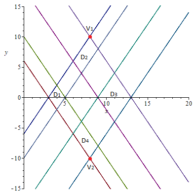
Figure 1. Support of $\mathcal{B}_{m}f$ with $m=0$, $I_{1}=\left[3,5\right]$, $I_{2}=\left[9,13\right]$.

With the notation of the figure, we see that $D_{1}$ and $D_{3}$ give account for the true frequencies of the signal, while $D_{2}$ and $D_{3}$ are non-zero interferences. A short computation shows that the coordinates of the two points $V_{1}$ and $V_{2}$ are

$$V_{1}=\left(\frac{2m+1}{2}\left(x_{2}+h_{2}\right)-\frac{2m-1}{2}x_{1},x_{1}-\left(x_{2}+h_{2}\right)\right),$$

$$V_{2}=\left(\frac{2m+1}{2}x_{1}-\frac{2m-1}{2}\left(x_{2}+h_{2}\right),\left(x_{2}+h_{2}\right)-x_{1}\right),$$

hence we see that the only effect of the perturbation parameter $m$ is the horizontal translation of the diamond’s corners, giving no room for damping. The only reduction procedure that can still be performed is the one proposed by Boggiatto et al. in [4], even if its validity is restricted to the special class of signals examined insofar. Furthermore, notice that we are in fact studying re-parametrized $\tau$-Wigner distributions in a broad sense, since now $m=\tau-(1/2)$ is free to run over $\mathbb{R}$. As already seen before and also noticeable from the coordinates of $V_{1}$ and $V_{2}$, when $m\in\mathbb{R}\setminus\left[-\tfrac{1}{2},\tfrac{1}{2}\right]$, the support of the signal is no longer conserved - neither in weak sense.

To conclude this section, we notice that an efficient reduction of interferences requires the Cohen’s kernel to show some decay at infinity - which is not the case of the chirp-like kernel $\theta_{M}$. In order to enhance this feature and at the same time to not lose other relevant ones satisfied by MWDs in the Cohen’s class, it seems reasonable to consider the Cohen’s distributions with kernels of type $\theta_{M}*\varphi$, where $\varphi\in\mathcal{S}^{\prime}\left({\mathbb{R}^{2d}}\right)$ is a decaying distribution satisfying suitable properties - for instance, one may ask that $\hat{\varphi}\left(\zeta_{1},\zeta_{2}\right)=\Phi\left(\zeta_{1}\cdot\zeta_{2}\right)$ with $\Phi\left(0\right)=1$ in order to keep the correct marginal densities. This kind of investigation deserves a special treatment in order to balance the trade-off between theoretically relevant features and practical purposes, thus it cannot be provided here. We confine ourselves to mention that choosing as smoothing distribution the one corresponding to the Born-Jordan kernel, namely

$$\varphi_{\sigma}\left(\zeta\right)=\hat{\varphi}\left(J\zeta\right)=\frac{\sin\left(\pi\zeta_{1}\zeta_{2}\right)}{\pi\zeta_{1}\zeta_{2}},\qquad\zeta=\left(\zeta_{1},\zeta_{2}\right)\in{\mathbb{R}^{2d}},$$

allows to enjoy some smoothing phenomena recently investigated, cf. for example [15, Theorem 4.1].

4.4. Continuity on functional spaces

In this section we prove that the continuity of bilinear distributions associated with matrices of Cohen’s type on modulation and Wiener amalgam spaces is a property stable under linear perturbations. We work with weights of polynomial type as in (11).

Theorem 4.12.

Let $A=A_{M}\in\mathrm{GL}\left(2d,\mathbb{\mathbb{R}}\right)$ be a Cohen-type matrix. Let $1\leq p_{i},q_{i},p,q<\infty$, $i=1,2$, such that

(35) $$p_{i},q_{i}\leq q,\qquad i=1,2,$$

and

(36) $$\frac{1}{p_{1}}+\frac{1}{p_{2}}\geq\frac{1}{p}+\frac{1}{q},\qquad\frac{1}{q_{1}}+\frac{1}{q_{2}}\geq\frac{1}{p}+\frac{1}{q}.$$

1. If $f_{1}\in M_{v_{\left|s\right|}}^{p_{1},q_{1}}\left(\mathbb{R}^{d}\right)$ and $f_{2}\in M_{v_{s}}^{p_{2},q_{2}}\left(\mathbb{R}^{d}\right)$, then $\mathcal{B}_{A}\left(f_{1},f_{2}\right)\in M_{1\otimes v_{s}}^{p,q}\left(\mathbb{R}^{2d}\right)$, and the following estimate holds:

   $$\left\|\mathcal{B}_{A}\left(f_{1},f_{2}\right)\right\|_{M_{1\otimes v_{s}}^{p,q}}\lesssim_{M}\left\|f_{1}\right\|_{M_{v_{\left|s\right|}}^{p_{1},q_{1}}}\left\|f_{2}\right\|_{M_{v_{s}}^{p_{2},q_{2}}}.$$

2. Assume further that both $M-\left(1/2\right)I$ and $M+\left(1/2\right)I$ are invertible (equivalently: $A_{M}$ is right-regular, or $P_{M}$ is invertible, cf. (33)). Set $v_{s}^{M}\equiv v_{s}\circ(I+P_{M}^{-1})^{-1}$. If $f_{1}\in M_{v_{\left|s\right|}}^{p_{1},q_{1}}\left(\mathbb{R}^{d}\right)$ and $f_{2}\in M_{v_{s}^{M}}^{p_{2},q_{2}}\left(\mathbb{R}^{d}\right)$, then $\mathcal{B}_{A}\left(f_{1},f_{2}\right)\in W\left(\mathcal{F}L^{p},L_{v_{s}^{M}}^{q}\right)\left(\mathbb{R}^{2d}\right)$, and the following estimate holds:

   $$\left\|\mathcal{B}_{A}\left(f_{1},f_{2}\right)\right\|_{W\left(\mathcal{F}L^{p},L_{v_{s}^{M}}^{q}\right)}\lesssim_{M}\left(C_{M}\right)^{1/q-1/p}\left\|f_{1}\right\|_{M_{v_{\left|s\right|}}^{p_{1},q_{1}}}\left\|f_{2}\right\|_{M_{v_{s}^{M}}^{p_{2},q_{2}}},$$

   where

   (37) $$C_{M}=\left|\det\left(M+\frac{1}{2}I\right)\det\left(M-\frac{1}{2}I\right)\right|>0.$$

Proof.

Fix $g\in\mathcal{S}\left(\mathbb{R}^{d}\right)$ and set $\Phi=\mathcal{B}_{A}g\in\mathcal{S}\left({\mathbb{R}^{2d}}\right)$. The key insight here is given by the short-time product formula in (27). Precisely, for any $z,\zeta\in{\mathbb{R}^{2d}}$ we have

$$\left|V_{\Phi}\mathcal{B}_{A}\left(f_{1},f_{2}\right)\left(z,\zeta\right)\right|=\left|V_{g}f_{1}\left(z+P_{M}J\zeta\right)\overline{V_{g}f_{2}\left(z+\left(I+P_{M}\right)J\zeta\right)}\right|,$$

where $P_{M}$ is the matrix defined in (33). Consequently, for $p,q<\infty$,

$$\left\|\mathcal{B}_{A}\left(f_{1},f_{2}\right)\right\|_{M_{1\otimes v_{s}}^{p,q}}$$

$$\asymp \left(\int_{{\mathbb{R}^{2d}}}\left(\int_{{\mathbb{R}^{2d}}}\left|V_{g}f_{1}\left(z+P_{M}J\zeta\right)\right|^{p}\left|V_{g}f_{2}\left(z+\left(I+P_{M}\right)J\zeta\right)\right|^{p}dz\right)^{q/p}v_{s}\left(J\zeta\right)^{q}d\zeta\right)^{1/q}.$$

The change of variables $z\mapsto z-\left(I+P_{M}\right)J\zeta$ turns the integral over $z$ into a convolution, then

$$\left\|\mathcal{B}_{A}\left(f_{1},f_{2}\right)\right\|_{M_{1\otimes v_{s}}^{p,q}} \asymp\left(\int_{{\mathbb{R}^{2d}}}\left(\left|V_{g}f_{2}\right|^{p}*\left|\left(V_{g}f_{1}\right)^{*}\right|^{p}\right)^{q/p}\left(J\zeta\right)v_{s}\left(J\zeta\right)^{q}d\zeta\right)^{1/q}$$

$$=\left\|\left|V_{g}f_{2}\right|^{p}*\left|\left(V_{g}f_{1}\right)^{*}\right|^{p}\right\|_{L_{v_{ps}}^{q/p}}^{1/p}.$$

From now on, the proof proceeds exactly as in [18, Theorem 3.1]. Similar arguments also hold whenever $p=\infty$ or $q=\infty$.

For what concerns boundedness on Wiener amalgam spaces, notice first that if $A_{M}$ is right regular, $\left(I+P_{M}\right)$ and also $\left(I+P_{M}^{-1}\right)$ are invertible, with

(38) $$\left(I+P_{M}^{-1}\right)^{-1}=\left(I+P_{M}\right)^{-1}P_{M}.$$

Therefore,

$$\left\|\mathcal{B}_{A}\left(f_{1},f_{2}\right)\right\|_{W\left(\mathcal{F}L^{p},L_{v_{s}\circ\left(I+P_{M}\right)^{-1}}^{q}\right)}$$

$$\asymp \left(\int_{\mathbb{R}^{2d}}\left(\int_{\mathbb{R}^{2d}}\left|V_{g}f_{1}\left(z+P_{M}J\zeta\right)\right|^{p}\left|V_{g}f_{2}\left(z+\left(I+P_{M}\right)J\zeta\right)\right|^{p}d\zeta\right)^{q/p}v_{s}\left(\left(I+P_{M}\right)^{-1}z\right)^{q}dz\right)^{1/q}.$$

Using the change of variables $\eta=z+P_{M}J\zeta$ and then the matrix equality (38), we can write

$$\left\|\mathcal{B}_{A}\left(f_{1},f_{2}\right)\right\|_{W\left(\mathcal{F}L^{p},L_{v_{s}\circ\left(I+P_{M}\right)^{-1}}^{q}\right)}$$

$$\asymp C_{M}^{-1/p}\left(\int_{\mathbb{R}^{2d}}\left(\int_{\mathbb{R}^{2d}}\left|V_{g}f_{1}\left(\eta\right)\right|^{p}\left|V_{g}f_{2}\left(\left(I+P_{M}^{-1}\right)\eta-P_{M}^{-1}z\right)\right|^{p}d\eta\right)^{q/p}\right.$$

$$\,\,\qquad\qquad\cdot\,\left.v_{s}\left(\left(I+P_{M}\right)^{-1}z\right)^{q}dz\right)^{1/q}$$

$$= C_{M}^{-1/p}\left(\int_{\mathbb{R}^{2d}}\left(\int_{\mathbb{R}^{2d}}\left|V_{g}f_{1}\left(\eta\right)\right|^{p}\left|V_{g}f_{2}\left(\left(I+P_{M}^{-1}\right)\left(\eta-\left(I+P_{M}^{-1}\right)^{-1}P_{M}^{-1}z\right)\right)\right|^{p}d\eta\right)^{q/p}\right.$$

$$\,\,\qquad\qquad\cdot\,\left.v_{s}\left(\left(I+P_{M}\right)^{-1}z\right)^{q}dz\right)^{1/q}$$

$$= C_{M}^{-1/p}\left(\int_{\mathbb{R}^{2d}}\left(\left|V_{g}f_{1}\right|^{p}*\left|\left((V_{g}f_{2})^{*}\left(\left(I+P_{M}^{-1}\right)\cdot\right)\right)^{*}\right|^{p}\right)^{q/p}\left(\left(I+P_{M}\right)^{-1}z\right)\right.$$

$$\,\,\qquad\qquad\cdot\,\left.v_{s}\left(\left(I+P_{M}\right)^{-1}z\right)^{q}dz\right)^{1/q}.$$

$$= C_{M}^{1/q-1/p}\left\|\left|V_{g}f_{1}\right|^{p}*\left|\left((V_{g}f_{2})^{*}\left(\left(I+P_{M}^{-1}\right)\cdot\right)\right)^{*}\right|^{p}\right\|_{L_{v_{ps}}^{q/p}}^{1/p},$$

where the constant $C_{M}$ is defined in (37) and we write $(V_{g}f_{2})^{*}(z)=(V_{g}f_{2})(-z)$. Again, the proof proceeds hereinafter as in [18, Theorem 3.1]. ∎

Remark 4.13.

We remark that the given estimates are not sharp, since we employed window functions depending on $M$ in order to perform the computations and thus the hidden constants in the symbol $\lesssim_{M}$ may depend on $M$. However, the comments of [18, Remark 3.2] are still valid here. In particular, the result holds for more general weight functions: for instance, sub-exponential weights or polynomial weights satisfying formula $\left(4.10\right)$ in [35] are suitable choices. Notice that the proof of the theorem in fact reduces to the study of continuity estimates for convolutions on weighted Lebesgue mixed-norm spaces. We would also point out that results in the spirit of Theorem 4.12(ii) have been already proved for $\tau$-Wigner distributions in [11, Lemma 3.1] and [19] and can be easily generalized to MWDs. In particular, we recover [19, Lemma 4.2] by noticing that $(I+P_{M})^{-1}=\mathcal{B}_{\tau}$ and $(I+P_{M}^{-1})^{-1}=\mathcal{U}_{\tau}$ for $M=(\tau-1/2)I$, where the matrices $\mathcal{B}_{\tau}$ and $\mathcal{U}_{\tau}$ are defined in [19, (5) and (26)].

Under more restrictive conditions on the Cohen-type matrix, namely assuming right-regularity (hence that both $M-(1/2)I$ and $M+(1/2)I$ are invertible), we are able to apply Proposition 3.9, obtaining boundedness results on Lebesgue spaces.

Theorem 4.14.

Let $A=A_{M}\in\mathrm{GL}\left(2d,\mathbb{R}\right)$ be a right-regular Cohen-type matrix. For any $1<p<\infty$ and $q\geq 2$ such that $q^{\prime}\leq p\leq q$, $f\in L^{p}\left(\mathbb{R}^{d}\right)$ and $g\in L^{p^{\prime}}\left(\mathbb{R}^{d}\right)$, the following facts hold.

1. $\mathcal{B}_{A}\left(f,g\right)\in L^{q}\left({\mathbb{R}^{2d}}\right)$, with

   $$\left\|\mathcal{B}_{A}\left(f,g\right)\right\|_{q}\leq\frac{\left\|f\right\|_{p}\left\|g\right\|_{p^{\prime}}}{\left|\det\left(M+\frac{1}{2}I\right)\right|^{\frac{1}{p}-\frac{1}{q}}\left|\det\left(M-\frac{1}{2}I\right)\right|^{\frac{1}{p^{\prime}}-\frac{1}{q}}}.$$

   In particular, $\mathcal{B}_{A}\left(f,g\right)$ is bounded $\left(q=\infty\right)$.

2. $\mathcal{B}_{A}\left(f,g\right)\in C_{0}\left({\mathbb{R}^{2d}}\right)$.

We remark that for MWDs in the Cohen’s class, a number of these properties still hold under the weaker assumption $M\in\mathrm{GL}\left(2d,\mathbb{R}\right)$. This is in fact a consequence of convolving with a bounded kernel $\theta_{M}\in L^{\infty}\left({\mathbb{R}^{2d}}\right)$.

References

- [1] Bayer, D.: Bilinear Time-Frequency Distributions and Pseudodifferential Operators. PhD Thesis, University of Vienna (2010)
- [2] Bényi, A., Grafakos, L., Gröchenig, K., and Okoudjou, K.: A class of Fourier multipliers for modulation spaces. Appl. Comput. Harmon. Anal. 19 (2005), no. 1, 131–139
- [3] Bényi, A., Gröchenig, K., Okoudjou, K., and Rogers, L. G.: Unimodular Fourier multipliers for modulation spaces. J. Funct. Anal. 246 (2007), no. 2, 366–384
- [4] Boggiatto, P., Carypis, E., and Oliaro, A.: Wigner representations associated with linear transformations of the time-frequency plane. In Pseudo-Differential Operators: Analysis, Applications and Computations (275-288), Springer (2011)
- [5] Boggiatto, P., De Donno, G., and Oliaro, A.: Weyl quantization of Lebesgue spaces. Math. Nachr. 282 (2009), no. 12, 1656–1663
- [6] Boggiatto, P., De Donno, G., and Oliaro, A.: Time-frequency representations of Wigner type and pseudo-differential operators. Trans. Amer. Math. Soc. 362 (2010), no. 9, 4955–4981
- [7] Boggiatto, P., De Donno, G., and Oliaro, A.: Hudson’s theorem for -Wigner transforms. Bull. Lond. Math. Soc. 45 (2013), no. 6, 1131–1147
- [8] Cohen, L.: Generalized phase-space distribution functions. J. Math. Phys. 7 (1996), no. 5, 781–786
- [9] Cohen, L.: Time-frequency Analysis. Prentice Hall (1995)
- [10] Cohen, L.: The Weyl Operator and its Generalization. Springer (2012)
- [11] Cordero, E., D’Elia, L., and Trapasso, S. I.: Norm estimates for -pseudodifferential operators in Wiener amalgam and modulation spaces. J. Math. Anal. Appl. 471 (2019), no. 1-2, 541–563
- [12] Cordero, E., De Gosson, M., Dörfler, M., and Nicola, F.: Generalized Born–Jordan Distributions and Applications. arXiv:1811.04601 [math.FA] (2018)
- [13] Cordero, E., De Gosson, M., Dörfler, M., and Nicola, F.: On the symplectic covariance and interferences of time-frequency distributions. SIAM J. Math. Anal. 50 (2018), no. 2, 2178–2193
- [14] Cordero, E., de Gosson, M., and Nicola, F.: Time-frequency analysis of Born-Jordan pseudodifferential operators. J. Funct. Anal. 272 (2017), no. 2, 577–598
- [15] Cordero, E., de Gosson, M., and Nicola, F.: On the reduction of the interferences in the Born-Jordan distribution. Appl. Comput. Harmon. Anal. 44 (2018), no. 2, 230–245
- [16] Cordero, E., Feichtinger, H.G., and Luef, F.: BBanach Gelfand triples for Gabor analysis. In Pseudo-differential Operators, 1–33, Lecture Notes in Math., 1949, Springer, Berlin, 2008.
- [17] Cordero, E., and Nicola, F.: Metaplectic representation on Wiener amalgam spaces and applications to the Schrödinger equation. J. Funct. Anal. 254 (2008), no. 2, 506–534
- [18] Cordero, E., and Nicola, F.: Sharp integral bounds for Wigner distributions. Int. Math. Res. Not. IMRN 2018, no. 6, 1779–1807
- [19] Cordero, E., Nicola, F., and Trapasso, S. I.: Almost diagonalization of -pseudodifferential operators with symbols in Wiener amalgam and modulation spaces. J. Fourier Anal. Appl. DOI: 10.1007/s00041-018-09651-z (2018)
- [20] de Gosson, M.: Symplectic Methods in Harmonic Analysis and in Mathematical Physics. Springer (2011)
- [21] de Gosson, M.: The Wigner Transform. World Scientific Publishing (2017)
- [22] Feichtinger, H. G.: Modulation spaces: looking back and ahead. Sampl. Theory Signal Image Process. 5 (2006), no. 2, 109–140
- [23] Feichtinger, H. G.: Banach convolution algebras of Wiener type. In Functions, series, operators, Vol. I, II (Budapest, 1980), 509–524, Colloq. Math. Soc. János Bolyai, 35, North-Holland, Amsterdam, 1983
- [24] Feichtinger, H. G., and Hörmann, W.: A distributional approach to generalized stochastic processes on locally compact Abelian groups. In New perspectives on approximation and sampling theory, 423–446, Appl. Numer. Harmon. Anal., Birkhäuser/Springer, Cham, 2014
- [25] Folland, G. B.: Harmonic Analysis in Phase Space. Princeton University Press (1989)
- [26] Golub, G. H. and Van Loan, C. F.: Matrix Computations (Vol. 3). Johns Hopkins University Press (2012)
- [27] Gröchenig, K.: Foundations of Time-frequency Analysis. Appl. Numer. Harmon. Anal., Birkhäuser (2001)
- [28] Gröchenig, K.: Time-frequency analysis of Sj strand’s class. Rev. Mat. Iberoam. 22 (2006), no. 2, 703–724
- [29] Hlawatsch, F., and Auger, F. (Eds.).: Time-frequency Analysis. John Wiley & Sons (2013)
- [30] Hlawatsch, F., and Boudreaux-Bartels, G. F.: Linear and quadratic time-frequency signal representations. IEEE Signal Proc. Mag. 9 (1992), no. 2, 21–67
- [31] Hörmann, W:. Generalized Stochastic Processes and Wigner Distribution. PhD thesis, University of Vienna (1989) 3
- [32] Hudson, R. L.: When is the Wigner quasi-probability density non-negative? Rep. Mathematical Phys. 6 (1974), no. 2, 249–252
- [33] Janssen, A. J. E. M.:A note on Hudson’s theorem about functions with nonnegative Wigner distributions. SIAM J. Math. Anal. 15 (1984), no. 1, 170–176
- [34] Janssen, A. J. E. M.: Positivity and spread of bilinear time-frequency distributions. In The Wigner distribution, 1–58, Elsevier Sci. B. V., Amsterdam, 1997
- [35] Toft, J.: Continuity properties for modulation spaces, with applications to pseudo-differential calculus. II. Ann. Global Anal. Geom. 26 (2004), no. 1, 73–106
- [36] Toft, J.: Matrix parameterized pseudo-differential calculi on modulation spaces. In Generalized Functions and Fourier Analysis, 215–235, Birkhäuser, 2017
- [37] Wong, M.W.: Weyl Transforms. Universitext. Springer-Verlag (1998)