Experimental Simultaneous Learning of Multiple Non-Classical Correlations

Abstract

Non-classical correlations can be regarded as resources for quantum information processing. However, the classification problem of non-classical correlations for quantum states remains a challenge, even for finite-size systems. Although there exist a set of criteria for determining individual non-classical correlations, a unified framework that is capable of simultaneously classifying multiple correlations is still missing. In this work, we experimentally explored the possibility of applying machine-learning methods for simultaneously identifying non-classical correlations. Specifically, by using partial information, we applied artificial neural network, support vector machine, and decision tree for learning entanglement, quantum steering, and non-locality. Overall, we found that for a family of quantum states, all three approaches can achieve high accuracy for the classification problem. Moreover, the run time of the machine-learning methods to output the state label is experimentally found to be significantly less than that of state tomography.

Introduction.—In 1935, Einstein, Podolsky, and Rosen (EPR) Einstein questioned the completeness of quantum mechanics (QM), as the theory seems to allow “spooky action at a distance” (known as EPR paradox). In quantum information science, much efforts have been devoted to achieve a deeper understanding of EPR’s paradox in terms of non-classical correlations, such as quantum entanglement Horodecki , EPR steering Brunner , and Bell non-locality Cavalcanti . The various relationships among different non-classical correlations not only shape the foundation of the quantum theory, but also find themselves many interesting applications.

The question is, how may one characterize the non-classical correlation for any given quantum state? To tackle such a problem, there are several challenges. (i) Even though various mathematical criteria and inequalities constraining non-classical correlations are known, for general multipartite states, the classification of entanglement, EPR steering, or Bell non-locality are generally computationally-hard problems Gurvits ; Huang ; Batle . (ii) Many existing methods require the information of the whole density matrix; experimentally, a full quantum state tomography would be required. (iii) Each type of non-classical correlation has a different set of criteria; it is not known whether one can, simultaneously, classify all the non-classical correlations, based on the same set of measurements or observables.

On the other hand, machine learning (ML) represents a branch of artificial intelligence, aiming at producing a predictive function or a computer program based on a set of training data Mitchell ; Devroye ; Vapnik ; Friedman . Beyond industrial applications, ML has created a profound impact on quantum information science, leading to a new research field, where many progresses have been achieved, including Hamiltonian learning Wiebe , automated quantum experiments search Krenn , identification of phase transition Schoenholz , topological phase of matter Zhang etc.

Recently, binary classification of quantum correlations have been achieved using the tools of ML, such as determination of entanglement Deng , and separability Lu ; Ma ; Jin . Our goal here is to take one step further and explore if ML can be applied, in both theoretical and experimental setting, to simultaneously characterize multiple non-classical correlations with only partial information about the given quantum state.

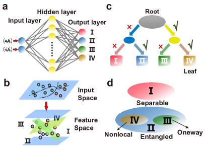
In addition to binary classifiers, we experimentally constructed a statistical unified witnesses for simultaneous characterizing different classes of multiple non-classical correlations through machine learning. Specifically, we compared three different multi-label state classifiers using three different ML methods (see FIG. 1), including artificial neural network (ANN), support vector machine (SVM) and decision tree (DT), where each classifier only takes partial information for each member in a family of quantum states. The label on the state is determined by using the positive partial transpose (PPT) criterion PPT , steering radius in two settings sun2016experimental and Clauser-Horne-Shimony-Holt (CHSH) inequalities CHSH , which are applied only to the training set but not the testing set.

Figure 1: Quantum correlation is divided into 4 categories by three typical ML models. a.The structures of artificial neural network (ANN). b. The support vector machine (SVM). c. The decision tree (DT). d. The Venn diagram of these four categories, in which I, II, III and IV represent the separable state, entangled state, one-way steerable state and Bell nonlocal state.

Labeling the training states.—For the purpose of demonstration, we shall focus on a family of quantum states, for which we can label unambiguously the class of non-classical correlations for each member. For feature extraction, we use partial information (two observables) of the quantum states, instead of the whole density matrix,

$$\langle{a}_{0}{b}^{\prime}_{0}\rangle,\langle{a}^{\prime}_{0}{b}_{0}\rangle,$$ (1)

to be the input, where ${a}_{0}={\sigma}_{z}$, ${a}^{\prime}_{0}={\sigma}_{x}$, ${b}_{0}=({\sigma}_{z}-{\sigma}_{x})/\sqrt{2}$, ${b}^{\prime}_{0}=({\sigma}_{z}+{\sigma}_{x})/\sqrt{2}$.

Figure 2: Experimental setup. A pair of polarization-entangled photons are generated in the preparation stage by pumping a type-II PPKTP crystal located in a Sagnac interferometer with an ultraviolet laser at 404 nm. The polarization state of the pump light is rotated by a half-wave plate (HWP₁). The dual-wavelength HWP₂ set to be $45^{\circ}$ in the Sagnac interferometer is used to exchange the polarizations of the pump light and down-converted photons. The HWP₃ set to be $45^{\circ}$ is used to change the form of the entangled state. One of the photons passes through an unbalanced interferometer and is sent to Alice. HWP₄ is set at $22.5^{\circ}$ and two sufficiently long calcite crystals (CCs) with the length of the last one being two times larger than the first one to completely destroy the coherence in different components. Two variable filters (VF, in red dotted line circle) are used to control the relative amplitudes between these two arms. The other photon is sent directly to Bob. Quarter-wave plates (QWPs), HWPs and polarization beam splitters (PBSs) on both sides of Alice and Bob are used for observables and tomography measurement. The photons are detected by single-photon detectors (SPDs), and the signals are sent for coincidence. The training and testing procedures are marked with black and red colors respectively. In the training case, criteria of quantum correlations are determined from tomographic data and the results are sent to the ML models together with the two characteristic features obtained from partial information measurement. In the testing case, only the two measured characteristic features are used to predict the labels.

Specifically, the family of quantum states under investigation is of the following form, which has been applied for demonstrating one-way steering oneway :

$$\rho_{AB}(p,\theta)=p|\psi_{\theta}\rangle\langle\psi_{\theta}|+(1-p)I_{A}/2\otimes\rho_{B}^{\theta},$$ (2)

where $|\psi_{\theta}\rangle=\cos\theta|00\rangle+\sin\theta|11\rangle$, and $\rho_{B}^{\theta}={\rm tr}_{A}(|\psi_{\theta}\rangle\langle\psi_{\theta}|)$. The members in the two-parameter family are characterized by the combination of the two parameters $\theta\in(0,2\pi)$, $p\in(0,1)$.

The non-classical correlations for the testing state $\rho_{AB}(p,\theta)$ can be determined by the following rules: (i) for separability, e.g. through PPT criterion, one can show that whenever $p<1/3$, the states are separable. Otherwise, they are entangled. (ii) for one-way steering, within the range, $1/\sqrt{2}<p<1/\sqrt{1+\sin^{2}2\theta}$, the states are one-way steerable J.Bowles . (iii) for non-locality, whenever $p>1/\sqrt{1+\sin^{2}2\theta}$, the states become non-local su2016beating . Each set of the features are associated with a label in the set I, II, III, IV, shown as FIG. 1d.

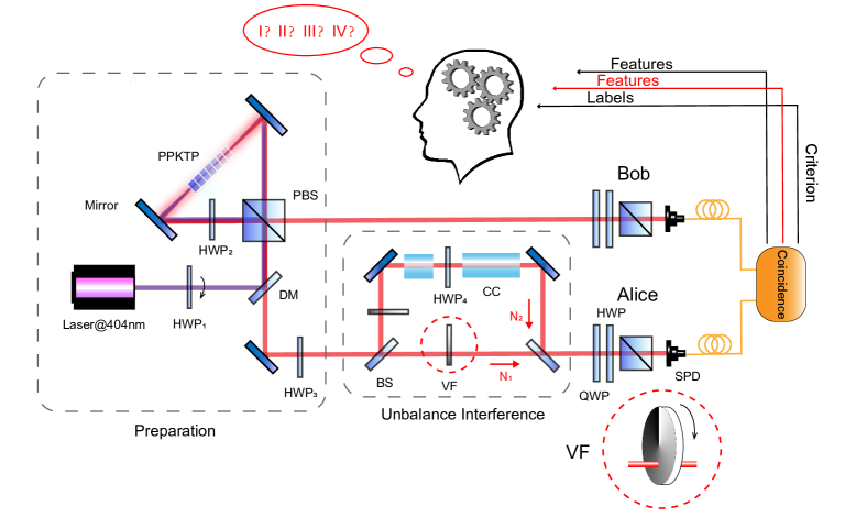
Experimental setting.—The experimental setup is shown in FIG. 2. Photon pairs entangled in the polarization basis $\{H,V\}$ ($H$ and $V$ represent horizontal and vertical polarization, respectively) are created through a type-II spontaneous parametric down conversion in a 20 mm-long periodical KTiOPO₄ (PPKTP) crystal, which is located on the Sagnac interferometer fedrizzi2007wavelength and pumped by a 404 nm continuous-wave diode laser. In order to generate the entangled state, $\cos\theta|HH\rangle+\sin\theta|VV\rangle$, a half-wave plate (HWP₁) is used to control the parameter $\theta$ by rotating the polarization of pump laser. One of the two photons is sent to an unbalanced interferometer (UI) while the other photon is sent to Bob directly.

In the UI, the photon is separated into two paths by a beam splitter (BS). The state in one of the paths remains unchanged. Two sufficiently long calcite crystals (CCs) with HWP₄ set to be $22.5^{\circ}$ between them are placed on the other path to completely destroy the coherence between different components. Two variable filters (VFs) are used to manipulate the relative photon counts ($N_{1}$, $N_{2}$) between these two paths, and the parameter $p$ can be demonstrated as $p=N_{1}/(N_{1}+N_{2})$. Combining these two paths into one, arbitrary two-qubit states $\rho_{AB}(p,\theta)$ can be prepared.

A quarter-wave plate (QWP), a HWP, and a polarization beam splitters (PBS) on both sides are used for quantum state tomography (16 projective measurements) and two characteristic observables (features, partial information) measurements (8 projective measurements). The integration time for each measurement is 5 s, and the maximal counts are about 60350. The labels can be deduced from the reconstructed density matrix $\rho_{AB}(p,\theta)$, by using PPT criteria, steering radius in two settings (see Supplementary Material (SM) supplementry for details) and CHSH inequalities. We implemented two independent experiments with different settings ($\theta_{2th}\to\theta_{1th}+\delta\theta$) to obtain a training set and a test set respectively, which are used to train and test the ML models.

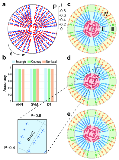
The fidelities (${Tr}[\sqrt{\sqrt{\rho_{AB}(p,\theta)}~{}\rho_{\rm exp}\sqrt{\rho_{AB}(p,\theta)}}]^{2}$) between the theoretical physical states $\rho_{AB}(p,\theta)$ and experimental states $\rho_{\rm exp}$ are higher than $99\%$, so that the reconstruction error of the matrix does not affect the labels of the states determined by the traditional criteria. To train the input data, we prepared 445 states as the training set (shown as blue dots in FIG. 3a in the $(p,\theta)$ space). For the trained models, we experimentally prepared a different set of 455 states for testing, which are shown as red dots in FIG. 3a. The $(p,\theta)$ are calculated through minimizing the value of $Tr[\rho_{AB}(p,\theta)-\rho_{\rm exp}]$.

Experimental results.—The two characteristic features of the testing states are then sent to different ML models. First, we consider applying the three ML models to perform binary classification (YES/NO labels). We found that the accuracy can reach more than $94\%$, which is comparable to that of a recent related experiment Jin . For example, when determining whether a state is separable or not, the accuracy of the ML models can reach over $97\%$. When applied to one-way steering and Bell non-locality, the prediction accuracies can be over $96\%$ and $94\%$, respectively. These results are shown in FIG. 3b.

Next, we consider applying the ML models to simultaneously label all four classes of states. The patterns of the states trained through ANN (see SM supplementry for the detailed structure), SVM and DT are shown in FIG. 3c, d and e. The accuracies are $90.11\%$, $90.11\%$ and $85.17\%$, respectively. States in red and blue colors are labeled to be separable and entangled, in green color are labeled to be one-way steerable and in yellow color are labeled to be Bell non-local, respectively. Error bars are estimated from the Poissonian counting statistics, which are smaller than the size of the dots. The inset in FIG. 3 is a magnification of the region in the black pane to exhibit error bars.

Gray lines in FIG. 3c-e represent the theoretical boundaries determined by the value of $p$ and $\theta$. Compared with the states labeled by traditional criteria, we can see that the prediction errors of ML models mainly occur at the boundaries, which are marked as “$\times$”. Since the calculation of steering radius is extremely sensitive when $\theta$ is close to 0, $\pi/2$, $\pi$ and $3\pi/2$, we omit these states in the test of the ability of the learning networks to reduce the errors induced by the physical criteria. A more detailed discussion is shown in SM supplementry .

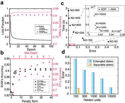
Data analysis.—The accuracy of the ML methods depends on the settings of several parameters, which are further investigated (see FIG. 4). The variations of the loss function and accuracy as a function of Epochs (stages) for the ANN is shown in FIG. 4a. The implementation of ANN is based on the TensorFlow API, where the loss function loss is defined by the categorical cross-entropy. The training process is to minimize the loss function by $RMSprop$ RMSprop . The accuracy is define as the proportion of the number of samples that are correctly labeled by ML models compared with traditional criteria. From the FIG. 4a, we found that the loss function decreases rapidly with the training accuracy growing quickly. An epoch is one complete presentation of the data set to be learned to a learning machine. In our work, we set max Epochs to 100. The value of loss function is 0.1477 and the training accuracy is $92.93\%$. The change of Epochs will cause slight disturbance to prediction accuracy. The value of $90.11\%$ is achieved when Epochs=30.

Figure 3: a. The training data (blue dots) and test data (red dots). b. The accuracies of ANN, SVM and DT, when distinguish whether a state is entangled, one-way steerable, or Bell nonlocal. The test results for multi-label classification with ANN, SVM and DT are shown in c., d. and e. with the accuracies of $90.11\%$, $90.11\%$ and $85.17\%$, respectively. The parameter $\theta$ varies from $0$ to $2\pi$ while the visibility $p$ changes from $0$ to $1$. The space is divided into four parts by the gray theoretical boundary, in which states in I, II, III and IV are theoretical predicted to be separable, entangled, one-way steerable and Bell nonlocal, respectively. “$\times$” represent the mistakenly labeled states via ML models compared with those labeled by traditional criteria. The error bars are smaller than the size of the dots. The inset shows the enlargement of the corresponding region in the black pane. The error bars are due to the Poissonian counting statistics.

We further analyzed the impact of penalty term penalty of SVM and DT’s maximum tree depth tree on the prediction accuracy, as shown in FIG. 4b. In the initial stage, with the increase of tree depth, the prediction ability becomes stronger for DT. When reaching the optimal depth 4, the DT prediction accuracy is $85.17\%$. Larger depth will make DT’s structure more complex and cause overfitting. The properties of SVM are similar to that of ANN. When penalty term is greater than 25, the prediction accuracy will converge to $90.11\%$. It’s due to the fact that the structure is not sensitive to penalty term in our task. See SM supplementry for the explanations of some jargons.

The run time is an important index to evaluate the performance of the ML algorithms. Given the same computing resources, state tomography requires about 5.28 s, while ANN costs about 0.33 s, and both SVM and DT take a very short time (10^-5 s) to output the label, indicating that ML models can significantly reduce the time complexity.

Figure 4: The comparison between three ML methods. a. The performance of ANN versus the Epochs. The black curves represent the value of the loss function and the red dotted line represents the training accuracy. Red triangles show the tested accuracy in different Epochs. b. The performance of DT and SVM versus max tree’s depth and error penalty factor with the data marked in black and red colors, respectively. Circles and triangles represent the training and testing results respectively. c. The relationship among labeling time, error and iterations (N2) of SDP (black); The relationship among labeling time, error and hidden units (N1) of ANN (red). d. The variation of error along with the number of hidden units for distinguishing entangled/separable states.

Scalability.—For systems with a higher dimension, e.g. a pair of qutrits, there is no known efficient way of labeling the training set. In this case, one may rely on numerical means, for example, semi-definite programming (SDP) Vandenberghe1996 for labeling. In the following, we shall demonstrate how our ML model can also be applied to learn the labels generated by SDP, using ANN on a pair qutrits.

In the following, we assume that SDP with 500 iterations for each data point (state) would be sufficient for separating the entangled states for a random set of states; For 100000 pairs of qubits, we found that the accuracy of SDP 500 can reach nearly $100\%$ compared with the PPT criterion. Furthermore, we studied the error and run time in classifying 768280 ($90\%$ training + $10\%$ testing) general 2-qutrit states labeled by SDP, which are equally divided between the entangle states and separable states. The result is shown in FIG. 4c (red points), where N1 is the number of hidden units representing the nerual nodes of the hidden layer in the neural network. For comparison, we also plot the run time and error relative to SDP 500 for SDP with different iterations N2 as black points in FIG. 4c. These results show that our ML model can efficiently learn SDP 500 with a small error.

We also analyze the main error sources of ANN. FIG. 4d illustrates the relationship between prediction error and hidden units for different types of 2-qutrit states (8000 entangle states + 12936 separable states). With the increase of hidden units, the entanglement/separable states error decrease. For the same number of hidden units, the ANN prediction error of entangled states is much larger than that of separable states. Therefore, the prediction error of neural network is mainly due to the inaccurate prediction of entangled states.

Conclusion.—In this work, we experimentally explored the possibility of the classification problem of multiple quantum correlations by comparing three ML approaches, namely ANN, SVM, and DT. It is shown that, all three methods can be experimentally trained to efficiently learn and classify quantum states, without state tomography.

Comparing these three ML methods with tomography and traditional criteria, we conclude that the predictive power is ordered as follows: by using the traditional criterion as the standard, ANN and SVM has higher accuracies than DT. In addition, ML models using only partial information of the state, which greatly reduces the number of projection measurements (8 projection measurements for ML features (observables) / 16 projection measurements for tomography in a 2-qubit system). Moreover, predictions of ML models have less time complexity.

Furthermore, we discuss the influence of the data source of the training set supplementry . It suggests the necessity of the experimental verification.