Design of Spectrally Shaped Binary Sequences
via Randomized Convex Relaxation

Abstract

Wideband communication receivers often deal with the problems of detecting weak signals from distant sources received together with strong nearby interferers. When the techniques of random modulation are used in communication system receivers, one can design a spectrally shaped sequence that mitigates interferer bands while preserving message bands. Common implementation constraints require sequence quantization, which turns the design problem formulation to an integer optimization problem solved using a semidefinite program on a matrix that is restricted to have rank one. Common approximation schemes for this problem are not amenable due to the distortion to the spectrum caused by the required quantization. We propose a method that leverages a randomized projection and quantization of the solution of a semidefinite program, an approach that has been previously used for related integer programs. We provide a theoretical and numerical analysis on the feasibility and quality of the approximation provided by the proposed approach. Furthermore, numerical simulations show that our proposed approach returns the same sequence as an exhaustive search (when feasible), showcasing its accuracy and efficiency. Furthermore, our proposed method succeeds in finding suitable spectrally shaped sequences for cases where exhaustive search is not feasible, achieving better performance than existing alternatives.

1 Introduction

Receivers for emerging wireless communication systems are expected to deal with a very wide spectrum and adaptively choose which parts of it to extract. The intense demand on the available spectrum for commercial users force many devices to share the spectrum [2, 3]. As a result, wideband communication systems have caused interference for applications using overlapping regions [4, 5]. Thus, a major issue for wideband communication receivers is to process spectra having very weak signals from a distant source mixed with strong signals from nearby sources. Practical nonlinearities in receiver circuits make the separation of such signals a key barrier for wideband communication systems since unfiltered interferers are large enough to cause distortion that can mask weaker signals.

Recently, random sequences for wideband signal modulation have been employed in the realization of communication system receivers [6, 7, 8]. In essence, the signal after random modulation contains a baseband spectrum that is the linear combination of all frequency components of the input signal. Thus, using a large enough number of modulation branches allows for successful recovery of the wideband signal, where the number of necessary branches is determined by the occupancy of the spectrum. The resulting multi-branch modulation system can be abstracted as an all-pass filter that preserves all frequency components of interest from the input signal.

In many cases, when the locations of one or more interferers is known, the modulation to null out the interferer band is desirable to reduce the distortion due to nonlinearities. Therefore, it is promising to replace the pseudo-random sequence with a spectrally shaped sequence that effectively implements a notch filter to suppress interferers. In addition to the strong interferer case described earlier, a similar problem arises in dynamic spectrum management (DSM), an approach that allows for flexibility in spectrum use. DSM attempts to determine the frequencies being used by previous or licensed applications and selects an optimal subset from the remaining frequencies for new or unlicensed applications. The signals for unlicensed applications should be optimized to minimize the interference with licensed signals while keeping their own capacities. More specifically, for Direct Sequence Spread Spectrum, a designed spreading code with particular spectral characteristic has been used to shape the unlicensed power spectra [9]. Another similar problem arises in active sensing, which obtains valuable information of targets or the propagation medium by sending probing waveforms toward an area of interest [10, 11, 12]. A well-designed waveform is crucial to the performance of active sensing.

To maximize the power efficiency in modulation, it is a standard requirement that the modulating waveform is constrained to be unimodular. Additionally, it is desirable that the waveform possess some specific spectrum magnitude. Such a choice improves the target detection performance in active sensing [13]. A common performance criterion gives preference to low autocorrelation sidelobes in the time domain or a flat spectrum in the frequency domain, since the autocorrelation function and the power spectral density form a Fourier transform pair. Metrics of low autocorrelation previously used in sequence design include the integrated sidelobe level (ISL) and the peak sidelobe level (PSL). Based on this relationship and these metrics, an iterative method has been developed to design unimodular waveforms with flat spectrum and impulse-like autocorrelation function by alternatively determining the waveform and an auxiliary phase [14, 15]. More recently, additional methods including majorization-minimization, coordinate descent, and alternating direction method of multipliers have been used in the literature to optimize the values of the ISL, PSL, and their weighted variants [16, 17, 18, 19, 20, 21].

Due to the fact that many devices are forced to coexist, the waveforms are constrained to have spectral nulls in specific bands to keep the mutual interference within acceptable levels. Based on the iterative method of [14, 15], the SHAPE algorithm designs sequences that simultaneously approach the desired spectrum magnitude and satisfy the envelope constraint [12, 3]. A sequence is obtained by alternatively searching the frequency and time domains to minimize the estimation error while meeting the two aforementioned criteria. In [22], a Lagrange programming neural network (LPNN) algorithm [23], based on nonlinear constrained optimization, is applied to design waveforms with unit modulus and spectral constrains. While it is possible to modify some of the algorithms in the literature to switch from an unimodular constraint to a binary constraint for the sequences, our numerical simulations in the sequel show that such changes result in significant performance losses in modulation.

In this work, we consider the problem of designing a binary sequence for modulation that is tailored for message preservation and interferer cancellation in order to allow for a simple system implementation [1]. More specifically, we aim to find binary sequences with sufficiently large spectrum magnitudes for the message band (i.e., for the frequencies where the message lies) while keeping sufficiently small magnitudes for the interferer band (i.e., frequencies where the interferer may exist). This design of spectrally shaped binary sequences can be formulated as a quadratically-constrained quadratic program (QCQP) with an objective function that measures message preservation and both equality constraints (for binary quantization) and inequality constraints (for interferer mitigation). This problem is NP-hard [24] and an exhaustive search for the optimal solution is computationally prohibitive beyond very small sequence lengths. It is well known that such an optimization problem can be written as a convex semidefinite program (SDP) with a non-convex rank-one constraint [25, 26]. Relaxing the SDP by dropping the rank constraint makes the problem solvable but also requires a procedure to reduce the SDP solution to a rank-one matrix in the highly likely case that the rank constraint is not met.

Goemans and Williamson [27] proposed a randomized projection and binary quantization method to provide improved approximations for the Maximum Cut problem, which is another important binary optimization problem involving a QCQP; however, the Maximum Cut problem features only equality constraints. The randomized projection returns a rank-one approximate solution that optimizes the value of the quadratic objective function in expectation. A best approximation is selected from repeated instances of the randomized projection by using a selection criterion. There exists a significant literature that has extended this method to approximately solve many similar optimization problems [28, 29, 30, 31, 32, 33, 24]. For example, the randomized projection is proven to approximately solve the QCQP with only inequality constraints [30, 32, 24] as well as the QCQP with both inequality constraints and equality constraints meeting a special diagonal structure [31, 33]. In the field of radar waveform design, the introduction of SDP relaxation and randomized projections has already shown that accurate and sometimes near-optimal approximations of complex-valued sequences are feasible [34, 35, 36, 37, 38]. However, the gap between the complex-valued sequence design in radar and the binary sequence design considered here prevents these analyses in the literature from applying on the problems we consider here.

In this paper, we present an algorithm to design binary sequences targeted to meet a specific spectrum shape. The algorithm is based on an SDP relaxation of a QCQP followed by a randomized projection and binary quantization, an approach that is inspired by [27]. Our main contributions can be detailed as follows. First, we propose a spectrally shaped binary sequence design approach based on optimization via a QCQP. Second, we extend the randomized projection and binary quantization method of [27] to our QCQP, which features both equality and inequality constraints. Third, we provide analytical and numerical results that study the feasibility of the sequences obtained from the proposed randomization, as well as the quality of the approximation achieved by the proposed algorithm. Fourth, we propose several custom score functions for the sequences obtained from randomization that allow for an improved selection of binary sequences that achieve both message preservation and interference rejection. Finally, we present numerical simulations that perform a comparison between an exhaustive search and the proposed sequence design method when the sizes that are sufficiently small to make exhaustive search feasible. The numerical results verify that our proposed method finds the optimal binary sequences. We also provide numerical simulations that show the advantages of the proposed algorithm against algorithms from the literature that have been modified when necessary to provide binary sequence designs.

This paper is organized as follows. In Section 2, we give a brief introduction to the SHAPE and LPNN algorithms for unimodular sequence design and present simple changes to both algorithms in order to make them suitable for binary sequence design. In Section 3, we provide a brief summary of QCQPs and existing approaches to solving QCQPs via SDP relaxation and randomized projection. In Section 4, we present and analyze the use of optimization and randomized projection to design spectrally shaped binary sequences; furthermore, we provide alternative criterion for sequence selection so that the resulting sequence allows for better interferer rejection. In Section 5, we present numerical simulations to validate the analysis in Section 4. Finally, we provide a discussion and conclusions in Section 6.

2 Background

To the best of our knowledge, there is no method in the literature that directly addresses the binary sequence design problem. Nonetheless, we summarize in this section two existing approaches for the problem of sequence design with unit modulus. We include those two approaches since they can be easily modified to design binary sequences by changing the optimization constraints. For other approaches to unimodular sequence design, such a change is not straightforward [34, 35, 36, 37, 38]. We will use the original and proposed modified algorithms for sequence design in the numerical simulations presented in Section 5.

2.1 SHAPE Algorithm

The SHAPE algorithm aims to find an unimodular sequence $s$ whose spectrum $vx$ has magnitude that meets both an upper bound $f_{i}$ and a lower bound $g_{i}$ ($i=1,2,\dots,N$), repectively [12, 3]:

$$\hat{\mathbf{s}}=\arg\min_{\mathbf{s},\mathbf{x}\in\mathbb{C}^{N},\alpha\in\mathbb{C}} \quad\|\mathcal{F}^{H}\mathbf{s}-\alpha\mathbf{x}\|_{2}^{2}$$

s.t. $$\quad|s_{i}|^{2}=1,i=1,2,\dots,N$$

$$\quad|x_{i}|\leq f_{i},i=1,2,\dots,N$$

$$\quad|x_{i}|\geq g_{i},i=1,2,\dots,N,$$ (1)

where $\mathcal{F}$ collects all elements of a discrete Fourier transform basis and $\alpha$ is a scalar factor accounting for the possible energy mismatch between the sequence and the constraints. The SHAPE algorithm solves (1) using an iterative approach with the following three main steps.

1. Given $\mathbf{s}$ and $\alpha$, find the spectrum $\mathbf{x}$:

   $$\hat{\mathbf{x}}=\arg\min_{\mathbf{x}\in\mathbb{C}^{N}} \quad\|\mathcal{F}^{H}\mathbf{s}-\alpha\mathbf{x}\|_{2}^{2}$$

   s.t. $$\quad|x_{i}|\leq f_{i},i=1,2,\dots,N$$

   $$\quad|x_{i}|\geq g_{i},i=1,2,\dots,N.$$ (2)

   The solution is given by

   $$\hat{x}_{i}=\left\{\begin{aligned} &f_{i}\frac{\mathcal{F}_{i}^{H}\mathbf{s}/\alpha}{\left|\mathcal{F}_{i}^{H}\mathbf{s}/\alpha\right|},&\left|\mathcal{F}_{i}^{H}\mathbf{s}/\alpha\right|>f_{i}\\ &g_{i}\frac{\mathcal{F}_{i}^{H}\mathbf{s}/\alpha}{\left|\mathcal{F}_{i}^{H}\mathbf{s}/\alpha\right|},&\left|\mathcal{F}_{i}^{H}\mathbf{s}/\alpha\right|<g_{i}\\ &\mathcal{F}_{i}^{H}\mathbf{s}/\alpha,&\text{otherwise}\end{aligned}\right.,$$ (3)

   $i=1,2,\dots,N$, where $\mathcal{F}_{i}$ denotes the $i^{\text{th}}$ column of $\mathcal{F}$.

2. Given $\mathbf{s}$ and $\mathbf{x}$, find the factor $\alpha$:

   $$\hat{\alpha}=\arg\min_{\alpha\in\mathbb{C}}\|\mathcal{F}^{H}\mathbf{s}-\alpha\mathbf{x}\|_{2}^{2}.$$ (4)

   The solution is given by

   $$\hat{\alpha}=\frac{\mathbf{x}^{H}\mathcal{F}^{H}\mathbf{s}}{\left\|\mathbf{x}\right\|_{2}^{2}}.$$ (5)

3. Given $\alpha$ and $\mathbf{x}$, find the sequence $\mathbf{s}$:

   $$\hat{\mathbf{s}}=\arg\min_{\mathbf{s}\in\mathbb{C}^{N}} \quad\left\|\mathcal{F}^{H}\mathbf{s}-\alpha\mathbf{x}\right\|_{2}^{2}$$

   s.t. $$\quad\left|s_{i}\right|^{2}=1,i=1,2,\dots,N.$$ (6)

   The solution is given by

   $$\hat{\mathbf{s}}_{i}=\frac{\alpha\mathcal{F}_{i}^{H}\mathbf{x}}{\left|\alpha\mathcal{F}_{i}^{H}\mathbf{x}\right|},i=1,2,\dots,N.$$ (7)

A straightforward change to the SHAPE algorithm for binary sequence design is to force the desired sequence $\mathbf{s}$ to be real in (1). This change is equivalent to replacing the optimization (6) with the binary constraint problem

$$\hat{\mathbf{s}}=\arg\min_{\mathbf{s}\in\mathbb{R}^{N}} \quad\left\|\mathcal{F}^{H}\mathbf{s}-\alpha\mathbf{x}\right\|_{2}^{2}$$

s.t. $$\quad\left|s_{i}\right|^{2}=1,i=1,2,\dots,N.$$ (8)

In other words, the resulting binary sequence can be obtained as

$$\hat{\mathbf{s}}_{i}=\operatorname{Sign}\left(\mathfrak{R}(\alpha\mathcal{F}_{i}^{H}\mathbf{x})\right),i=1,2,\dots,N,$$ (9)

where $\mathfrak{R}(\cdot)$ denotes the real part of a complex number and $\operatorname{Sign}\left(\cdot\right)$ denotes the sign of a real number.

2.2 LPNN Algorithm

In [22], a Lagrange programming neural network (LPNN) for unimodular sequence design with target spectrum $\mathbf{x}$ is formulated as follows:

$$\hat{\mathbf{s}}=\arg\min_{\mathbf{s}\in\mathbb{C}^{N},\alpha\in\mathbb{R}} \quad\sum_{i=1}^{N}w_{i}{\left(\left|\mathcal{F}_{i}^{H}\mathbf{s}\right|^{2}-\alpha x_{i}\right)}^{2}+c_{0}\sum_{i=1}^{N}{\left(\left|\mathbf{e}_{i}^{T}\mathbf{s}\right|^{2}-1\right)}^{2}$$

s.t. $$\quad\left|\mathbf{e}_{i}^{T}\mathbf{s}\right|^{2}=1,i=1,2,\dots,N.$$ (10)

Here $\mathbf{e}_{i}$ denotes the canonical column vector whose $i^{\text{th}}$ entry is $1$ and others are $0$, and $w_{i}$ are weights for each frequency component. The second term in the objective function is the augmented term to improve the algorithm’s convexity and stability. By separating the real and imaginary parts of the matrices and vectors in the equation as

$$\mathbf{t}=\begin{bmatrix}\mathfrak{R}\{\mathbf{s}\}\\ \mathfrak{I}\{\mathbf{s}\}\end{bmatrix},\quad\mathbf{F}_{i}=\begin{bmatrix}\mathfrak{R}\{\mathcal{F}_{i}\}&\mathfrak{I}\{\mathcal{F}_{i}\}\\ -\mathfrak{I}\{\mathcal{F}_{i}\}&\mathfrak{R}\{\mathcal{F}_{i}\}\end{bmatrix},\quad\mathbf{E}_{i}=\begin{bmatrix}\mathbf{e}_{i}&\mathbf{0}\\ \mathbf{0}&\mathbf{e}_{i}\end{bmatrix},$$

the complex-valued optimization (10) is transformed into the real-valued optimization

$$\min_{\mathbf{t}\in\mathbb{R}^{2N},\alpha\in\mathbb{R}} \quad\sum_{i=1}^{N}w_{i}{\left(\mathbf{t}^{T}\mathbf{F}_{i}\mathbf{F}_{i}^{T}\mathbf{t}-\alpha x_{i}\right)}^{2}+\quad c_{0}\sum_{i=1}^{N}{\left(\mathbf{t}^{T}\mathbf{E}_{i}\mathbf{E}_{i}^{T}\mathbf{t}-1\right)}^{2}$$

s.t. $$\quad\mathbf{t}^{T}\mathbf{E}_{i}\mathbf{E}_{i}^{T}\mathbf{t}=1,i=1,2,\dots,N.$$ (11)

The Lagrangian function for this problem is set up as

$$\mathcal{L}\left(\mathbf{t},\alpha,\boldsymbol{\mu}\right) =\sum_{i=1}^{N}w_{i}{\left(\mathbf{t}^{T}\mathbf{F}_{i}\mathbf{F}_{i}^{T}\mathbf{t}-\alpha x_{i}\right)}^{2}+c_{0}\sum_{i=1}^{N}{\left(\mathbf{t}^{T}\mathbf{E}_{i}\mathbf{E}_{i}^{T}\mathbf{t}-1\right)}^{2}+\sum_{i=1}^{N}\mu_{i}\left(\mathbf{t}^{T}\mathbf{E}_{i}\mathbf{E}_{i}^{T}\mathbf{t}-1\right),$$ (12)

where $\mu_{i}$ is the Lagrange multiplier. The LPNN then computes increments for the parameters and solution of this problem as follows:

$$\Delta\mathbf{t} =-\frac{\partial\mathcal{L}}{\partial\mathbf{t}}=-4\sum_{i=1}^{N}w_{i}\left(\mathbf{t}^{T}\mathbf{F}_{i}\mathbf{F}_{i}^{T}\bar{s}-\alpha x_{i}\right)\mathbf{F}_{i}\mathbf{F}_{i}^{T}-4c_{0}\sum_{i=1}^{N}\left(\mathbf{t}^{T}\mathbf{E}_{i}\mathbf{E}_{i}^{T}\mathbf{t}-1\right)\mathbf{E}_{i}\mathbf{E}_{i}^{T}-2\sum_{i=1}^{N}\mu_{i}\mathbf{E}_{i}\mathbf{E}_{i}^{T}\mathbf{t},$$ (13)

$$\Delta\alpha =-\frac{\partial\mathcal{L}}{\partial\alpha}=2\sum_{i=1}^{N}w_{i}\left(\mathbf{t}^{T}\mathbf{F}_{i}\mathbf{F}_{i}^{T}\mathbf{t}-\alpha x_{i}\right)x_{i},$$ (14)

$$\Delta\mu_{i} =-\frac{\partial\mathcal{L}}{\partial\mu_{i}}=\mathbf{t}^{T}\mathbf{E}_{i}\mathbf{E}_{i}^{T}\mathbf{t}-1.$$ (15)

The LPNN algorithm initializes the so-called neurons $\mathbf{t}$, $\alpha$, $\boldsymbol{\mu}$ randomly. The neurons are updated using the increments above at each iteration $k$:

$$\mathbf{t}^{k+1} =\mathbf{t}^{k}+\rho\Delta\mathbf{t},$$ (16)

$$\alpha^{k+1} =\alpha^{k}+\rho\Delta\alpha,$$ (17)

$$\boldsymbol{\mu}^{k+1} =\boldsymbol{\mu}^{k}+\rho\Delta\boldsymbol{\mu}.$$ (18)

Finally, the unimodular sequence $\hat{\mathbf{s}}$ is constructed by taking first and last $N$ entries of $\bar{s}$ as its real and imaginary parts, respectively.

The LPNN algorithm can be modified to provide binary sequences by changing the $s\in\mathbb{C}^{N}$ constraint in (10) to $s\in\mathbb{R}^{N}$, making (10) a real-valued optimization. Thus, we can directly obtain the dynamics for the neurons $s$, $\alpha$, and $\mu$ by replacing $\mathbf{t}$ to $\mathbf{s}$, $\mathbf{F}_{i}$ and $\mathbf{F}_{i}^{T}$ to $\mathcal{F}_{i}$ and $\mathcal{F}_{i}^{H}$, and $\mathbf{E}_{i}$ to $\mathbf{e}_{i}$ in (13-18).

3 Quadratically Constrained Quadratic Programming

In this section, we summarize approaches to approximately solve QCQPs and provide available analytical frameworks for the approximation performance. The approaches described in this section originate from the seminal paper [27], with extensions to several related problems [28, 29, 30, 31, 32, 33, 24]. In general, a QCQP problem can be written as

$$\hat{\mathbf{s}}=\arg\max_{\mathbf{s}\in\mathbb{R}^{N}}\quad f\left(\mathbf{s}\right) =\mathbf{s}^{T}\mathbf{A}\mathbf{s}$$

$$\text{s.t.}\quad g_{k}\left(\mathbf{s}\right) =\mathbf{s}^{T}\mathbf{B}_{k}\mathbf{s}\leq\alpha_{k},\quad k\in\mathcal{I},$$

$$h_{k}\left(\mathbf{s}\right) =\mathbf{s}^{T}\mathbf{C}_{k}\mathbf{s}=\beta_{k},\quad k\in\mathcal{E},$$ (19)

where $\mathbf{A}$, $\mathbf{B}_{k}$ and $\mathbf{C}_{k}$ are characteristic matrices for the objective function $f$, the inequality constraint function $g_{k}$ and the equality constraint function $h_{k}$, respectively. Specific instances of this QCQP, placing different conditions in the involved matrices, have been studied in the literature; we focus on the following specific classes.

1. There are no inequality constraints (i.e., $|\mathcal{I}|=0$), $|\mathcal{E}|=N$, and $\mathbf{C}_{k}=\mathbf{e}_{k}\mathbf{e}_{k}^{T}$. When all $\beta_{k}=1$, the equality constraints essentially enforce a binary constraint to the solution $s$, which has been used to solve the Maximum Cut problem [27, 35, 37].

2. There are no equality constraints (i.e., $|\mathcal{E}|=0$) and $\mathbf{B}_{k}$ are all positive semidefinite. The feasible set $\{\mathbf{s}|\mathbf{s}^{T}\mathbf{B}_{k}\mathbf{s}\leq\alpha_{k},k\in\mathcal{I}\}$ is an intersection of ellipsoids with common center [30, 32, 24, 38].

3. There is only one inequality constraint and the characteristic matrix $\mathbf{B}$ is diagonal, $|\mathcal{E}|=N$, and $\mathbf{C}_{k}=\mathbf{e}_{k}\mathbf{e}_{k}^{T}$ [31, 33, 36]. This class is equivalent to the first class when the feasible set is not empty, due to the fact that any solution that satisfies the equality constraints (and thus is a vertex of a high-dimensional hypercube) will always lie inside the high-dimensional ball described by the inequality constraint.

We will show in the sequel that the proposed binary sequence design can be formed as a QCQP with both equality constraints and inequality constraints with more general structure, thus not belong to any of the three classes described here.

3.1 Semidefinite Programming Relaxation

Solving a QCQP is NP-hard [24]. Most optimization methods for QCQP are based on a relaxation of the problems where an upper bound of of the objective value for the optimal solution is computed. The SDP relaxation has been an attractive approach due to its potential to find a good approximate solution for many QCQPs, including the specific classes mentioned above.

By lifting $\mathbf{s}$ to a symmetric matrix $\mathbf{S}=\mathbf{s}\mathbf{s}^{T}\in\mathbb{R}^{N\times N}$ with $\operatorname{Rank}\left(\mathbf{S}\right)=1$, the objective function $f$ in (19) has a linear representation with respect to $\mathbf{S}$. Therefore, the QCQP in (19) can be expressed equivalently as

$$\widehat{\mathbf{S}}=\arg\max_{\mathbf{S}\in\mathbb{S}^{N}}\quad \operatorname{Trace}\left(\mathbf{A}\mathbf{S}\right)$$

s.t. $$\operatorname{Trace}\left(\mathbf{B}_{k}\mathbf{S}\right)\leq\alpha_{k},\quad k\in\mathcal{I},$$

$$\operatorname{Trace}\left(\mathbf{C}_{k}\mathbf{S}\right)=\beta_{k},\quad k\in\mathcal{E},$$

$$\operatorname{Rank}\left(\mathbf{S}\right)=1,$$ (20)

where $\mathbb{S}^{N}$ represents the set of all $N$-dimensional positive semidefinite matrices. Given that such matrices are positive semidefinite and rank-one, any feasible solution $\mathbf{S}$ to (20) can be factorized as $\mathbf{s}\mathbf{s}^{T}$ such that $\mathbf{s}$ is an feasible solution to (19).

Though (20) is as difficult to solve as (19), it indicates that the only non-convex constraint is the rank constraint and that the objective function and all other constraints are convex with respect to $\mathbf{S}$ when $\mathbf{A}$, $\mathbf{B}_{k}$, and $\mathbf{C}_{k}$ are all positive semidefinite. Thus the SDP relaxation of (19) is obtained by dropping the rank constraint:

$$\widehat{\mathbf{S}}=\arg\max_{\mathbf{S}\in\mathbb{S}^{N}}\quad f\left(\mathbf{S}\right) =\operatorname{Trace}\left(\mathbf{A}\mathbf{S}\right)$$

$$\text{s.t.}\quad g_{k}\left(\mathbf{S}\right) =\operatorname{Trace}\left(\mathbf{B}_{k}\mathbf{S}\right)\leq\alpha_{k},\quad k\in\mathcal{I},$$

$$h_{k}\left(\mathbf{S}\right) =\operatorname{Trace}\left(\mathbf{C}_{k}\mathbf{S}\right)=\beta_{k},\quad k\in\mathcal{E}.$$ (21)

The resulting convex problem (21) can be efficiently solved, e.g., by interior-point methods [39].

3.2 Randomized Projection

After solving the SDP relaxation, the next important step is to extract a feasible solution $\tilde{\mathbf{s}}$ to (19) from the optimal solution $\widehat{\mathbf{S}}$ resulting from (21). If $\widehat{\mathbf{S}}$ is rank-one, then $\widehat{\mathbf{S}}$ is also the optimal solution to (20) and one can obtain an optimal solution $\tilde{\mathbf{s}}$ to (19) by factorizing $\widehat{\mathbf{S}}=\tilde{\mathbf{s}}\tilde{\mathbf{s}}^{T}$. Otherwise, if the rank of $\widehat{\mathbf{S}}$ is larger than one, then we need to obtain a vector $\tilde{\mathbf{s}}$ such that the outer product $\tilde{\mathbf{s}}\tilde{\mathbf{s}}^{T}$ is close to $\widehat{\mathbf{S}}$ while $\tilde{\mathbf{s}}$ remains feasible to (19). However, in general, the obtained feasible solution $\tilde{\mathbf{s}}$ will not be the optimal solution.

It is natural to use the principal eigenvector of $\widehat{\mathbf{S}}$, the eigenvector corresponding to the eigenvalue with largest magnitude, to build the rank-one approximation. Specifically, when $\operatorname{Rank}\left(\widehat{\mathbf{S}}\right)=R$, then $\widehat{\mathbf{S}}$ has $r$ eigenvalues $\lambda_{1}\geq\lambda_{2}\geq\cdots\geq\lambda_{R}>0$ and eigenvectors $\mathbf{u}_{1},\mathbf{u}_{2},\ldots,\mathbf{u}_{r}\in\mathbb{R}^{N}$ such that the eigen-decomposition is $\widehat{\mathbf{S}}=\sum_{k=1}^{R}\lambda_{k}\mathbf{u}_{k}\mathbf{u}_{k}^{T}=\mathbf{U}\boldsymbol{\Sigma}\mathbf{U}^{T}$, where $\mathbf{U}=\left[\mathbf{u}_{1},\mathbf{u}_{2},\ldots,\mathbf{u}_{r}\right]$ and $\boldsymbol{\Sigma}$ is the diagonal matrix with $\operatorname{Diag}\left(\boldsymbol{\Sigma}\right)={\left[\lambda_{1},\lambda_{2},\ldots,\lambda_{r}\right]}^{T}$. Since $\lambda_{1}\mathbf{u}_{1}\mathbf{u}_{1}^{T}$ is the best rank one approximation of $\widehat{\mathbf{S}}$ in the Frobenius norm sense, $\mathbf{w}=\sqrt{\lambda_{1}}\mathbf{u}_{1}$ can be a candidate solution to problem (19), provided that it remains feasible.

Randomization is another way to perform the rank-one approximation. Assume that $\mathbf{v}\in\mathbb{R}^{R}$ is a random vector whose entries are drawn independently and identically according to the standard Gaussian distribution, i.e., $\mathbf{v}\sim\mathcal{N}\left(\mathbf{0},\mathbf{I}\right)$, where $\mathbf{I}$ is the identity matrix. Let $\mathbf{w}=\mathbf{U}\boldsymbol{\Sigma}^{1/2}\mathbf{v}$, where $\boldsymbol{\Sigma}^{1/2}$ is the element-wise square root of $\boldsymbol{\Sigma}$. A simple calculation indicates that $\mathbb{E}\left(\mathbf{w}\mathbf{w}^{T}\right)=\widehat{\mathbf{S}}$, where $\mathbb{E}\left(\cdot\right)$ returns the element-wise expectation. Furthermore, we have $\mathbb{E}\left(\mathbf{w}^{T}\mathbf{A}\mathbf{w}\right)=\mathbb{E}\left(\operatorname{Trace}\left(\mathbf{A}\mathbf{w}\mathbf{w}^{T}\right)\right)=\operatorname{Trace}\left(\mathbf{A}\widehat{\mathbf{S}}\right)$. Finally, we have $\mathbb{E}\left(\mathbf{w}^{T}\mathbf{B}_{k}\mathbf{w}\right)=\operatorname{Trace}\left(\mathbf{B}_{k}\widehat{\mathbf{S}}\right)$ and $\mathbb{E}\left(\mathbf{w}^{T}\mathbf{C}_{k}\mathbf{w}\right)=\operatorname{Trace}\left(\mathbf{C}_{k}\widehat{\mathbf{S}}\right)$. Thus $\mathbf{w}$ maximizes the expected value of the objective function in (19) and satisfies the corresponding constraints in expectation. In other words, the SDP relaxation in (21) is equivalent to the following stochastic QCQP:

$$\widehat{\mathbf{S}}=\arg\max_{\mathbf{S}\in\mathbb{S}^{N}}\quad \mathbb{E}\left(\mathbf{w}^{T}\mathbf{A}\mathbf{w}\right)$$

s.t. $$\mathbb{E}\left(\mathbf{w}^{T}\mathbf{B}_{k}\mathbf{w}\right)\leq\alpha_{k},\quad k\in\mathcal{I},$$

$$\mathbb{E}\left(\mathbf{w}^{T}\mathbf{C}_{k}\mathbf{w}\right)=\beta_{k},\quad k\in\mathcal{E},$$

$$\mathbf{w}\sim\mathcal{N}\left(\mathbf{0},\mathbf{S}\right).$$ (22)

Such stochastic interpretation of the SDP relaxation provides an alternative way to generate the rank-one approximated solution to (21).

However, both the approximated solutions $\mathbf{w}$ from the eigen-decomposition and the randomized projection may not be feasible for the original QCQP. A feasible solution $\tilde{\mathbf{s}}$ can be obtained by projecting the approximated solution $\mathbf{w}$ onto the feasible solution set such that $\tilde{\mathbf{s}}$ is the nearest feasible solution to $\mathbf{w}$. For example, the feasible solutions for QCQP classes I and III are obtained by the element-wise multiplication $\tilde{s}_{k}=\operatorname{Sign}\left(w_{k}\right)\cdot\beta_{k}$ ($k=1,2,\dots,N$), where $\tilde{s}_{k}$ and $w_{k}$ denote the $k^{\mathrm{th}}$ entries of $\tilde{\mathbf{s}}$ and $\mathbf{w}$, respectively [31, 33]. As a special case of QCQP class I, the feasible solutions for QCQPs under binary constraints (i.e., all $\beta_{k}=1$) are obtained via binary quantization $\tilde{\mathbf{s}}=\operatorname{Sign}\left(\mathbf{w}\right)$, where $\operatorname{Sign}\left(\mathbf{w}\right)$ returns the signs of all entries of $\mathbf{w}$ [27]. Alternatively, $\tilde{\mathbf{s}}=\mathbf{w}\max_{k\in\mathcal{I}}\sqrt{\alpha_{k}/\left(\mathbf{w}^{T}\mathbf{B}_{k}\mathbf{w}\right)}$ has been used to obtain feasible solutions for QCQP class II [32].

Although leveraging the principal eigenvector of $\widehat{\mathbf{S}}$ is another simple way of applying rank-one approximation to $\widehat{\mathbf{S}}$, such an approach is not suitable for problems featuring additional constraints. More specifically, when binary constraints are included and the principal eigenvector is found to meet the inequality constraint, the binary quantization will likely affect the optimality and feasibility of the approximate solution. Additionally, as shown in the sequel, the quantized principal eigenvector provides performance worse than that obtained by the sequence given by our randomized approach.

3.3 Approximation Ratio

The goal of the SDP relaxation (21) is to obtain the candidate solution $\tilde{\mathbf{s}}$ for problem (19) that is as close to the optimal solution $\hat{\mathbf{s}}$ as possible. Since any optimal solution $\hat{\mathbf{s}}$ to the QCQP (19) can produce a feasible solution $\hat{\mathbf{s}}\hat{\mathbf{s}}^{T}$ to the SDP relaxation (21), we have $f(\hat{\mathbf{s}})\leq f(\widehat{\mathbf{S}})$, where $\widehat{\mathbf{S}}$ represents the optimal solution to the SDP relaxation (21). Additionally, $f(\tilde{\mathbf{s}})\leq f(\hat{\mathbf{s}})$ due to the fact that the solution $\tilde{\mathbf{s}}$ resulting from the relaxation solution $\widehat{\mathbf{S}}$ by any method should be feasible to the original problem (19). Based on these relationships, if $\gamma=f(\tilde{\mathbf{s}})/f(\widehat{\mathbf{S}})$ is the ratio between the objective function for a feasible solution $\tilde{\mathbf{s}}$ obtained by a rank-one approximation method and the objective function value for the SDP relaxation optimal solution $\widehat{\mathbf{S}}$, then this performance ratio is no smaller than that for $\hat{\mathbf{s}}$ with the same factor:

$$\gamma=\frac{f(\tilde{\mathbf{s}})}{f(\widehat{\mathbf{S}})}\leq\frac{f(\tilde{\mathbf{s}})}{f(\hat{\mathbf{s}})}\leq 1.$$ (23)

The factor $\gamma$ measures not only how good the approximation method is but also how close the resulting solution is to the optimal solution in terms of the objective function’s value.

The SDP relaxation with randomized projection provides guaranteed approximation ratios for many QCQP problems. For example, such a scheme generates an approximation algorithm for the Maximum Cut problem (belonging to class I), with $\gamma\geq 0.87$ [27].

4 Spectrally Shaped Binary Sequence Design

In this section, we develop an efficient method to generate a binary sequence that is based on the SDP relaxation and randomized projection introduced in Section 3. A filter implemented to have such a sequence as its impulse response provides a frequency response with a bandpass and a notch for the message and interferer bands, respectively. We also provide a theoretical analysis of the algorithm to show its approximation ratio and the likelihood of feasibility for the randomized sequences obtained. To improve the performance of the algorithm, we end the section with a discussion on possible additional criteria to select among the multiple sequences obtained via the proposed randomization.

4.1 Design Algorithm

We desire for the spectrally shaped sequence to provide a passband and notch for the pre-determined message and interferer bands, respectively. We denote by $\mathcal{F}_{M}$ and $\mathcal{F}_{I}$ the collection of all discrete Fourier transform basis elements corresponding to the message band $\Omega_{M}\subseteq\{1,2,\dots,N\}$ and interferer band $\Omega_{I}\subseteq\{1,2,\dots,N\}$, respectively. We also assume that $\Omega_{M}\cap\Omega_{I}=\emptyset$, but we do not place any other restrictions on the message and interferer bands. An optimization-based approach for the design of an $N$-point spectrally shaped binary sequence can be written as the QCQP

$$\hat{\mathbf{s}}=\arg\max_{\mathbf{s}\in\mathbb{R}^{N}}\quad f(\mathbf{s}) =\left\|\mathcal{F}_{M}^{H}\mathbf{s}\right\|_{2}^{2}$$

$$\text{s.t.}\quad g(\mathbf{s}) =\left\|\mathcal{F}_{I}^{H}\mathbf{s}\right\|_{2}^{2}\leq\alpha,$$

$$h_{k}(\mathbf{s}) =s^{2}_{k}=1,\quad k=1,2,\dots,N,$$ (24)

for some interferer tolerance $\alpha>0$, where $s_{k}$ denotes the $k^{\mathrm{th}}$ entry of $\mathbf{s}$. As mentioned in Section 3, such an integer optimization problem is NP-hard. Though it is possible to use an exhaustive method that searches over all possible binary sequences to return the optimal sequence when the sequence length is very small, it is too inefficient and even impossible to use the exhaustive method when the sequence length is relatively large.

Following the framework prescribed in Section 3, the SDP relaxation for the QCQP (24) can be obtained by noting that $\left\|\mathcal{F}_{M}^{H}\mathbf{s}\right\|_{2}^{2}=\operatorname{Trace}\left(\mathcal{F}_{M}\mathcal{F}_{M}^{H}\mathbf{s}\mathbf{s}^{T}\right)$ and $\left\|\mathcal{F}_{I}^{H}s\right\|_{2}^{2}=\operatorname{Trace}\left(\mathcal{F}_{I}\mathcal{F}_{I}^{H}\mathbf{s}\mathbf{s}^{T}\right)$, providing us with the optimization

$$\widehat{\mathbf{S}}=\arg\max_{\mathbf{S}\in\mathbb{S}^{N}}\quad f\left(\mathbf{S}\right) =\operatorname{Trace}\left(\mathcal{F}_{M}\mathcal{F}_{M}^{H}\mathbf{S}\right)$$

$$\text{s.t.}\quad g\left(\mathbf{S}\right) =\operatorname{Trace}\left(\mathcal{F}_{I}\mathcal{F}_{I}^{H}\mathbf{S}\right)\leq\alpha/2,$$

$$h_{k}\left(\mathbf{S}\right) =s_{k,k}=1,\quad k=1,2,\ldots,N,$$ (25)

where $s_{k,k}$ denotes the $k^{\mathrm{th}}$ diagonal entry of $\mathbf{S}$. Note that we omit the redundant operations that take the real part of $f\left(\mathbf{S}\right)$ and $g\left(\mathbf{S}\right)$ since both $\mathcal{F}_{M}\mathcal{F}_{M}^{H}$ and $\mathcal{F}_{M}\mathcal{F}_{I}^{H}$ are Hermitian and these quadratic functions will always be real-valued. Note also that the bound on the inequality constraint has been halved in the SDP relaxation in order to provide a theoretical guarantee later in this section.

Our proposed SDP approximation and randomization for the QCQP is detailed in Algorithm 1. After obtaining and decomposing the optimal solution $\widehat{\mathbf{S}}$ for the SDP relaxation, a randomly generated vector $\mathbf{v}$ is used to project $\widehat{\mathbf{S}}$ from a high dimensional space to a low dimensional space and obtain the approximation vector $\mathbf{w}_{\ell}$. A candidate binary sequence $\tilde{\mathbf{s}}_{\ell}$ is then obtained by quantizing the approximation vector $\mathbf{w}_{\ell}$. The algorithm repeats the random projection $L$ times to provide a set of candidate sequences and finally outputs the sequence that maximizes the message band power while meeting the requested upper bound for the interferer band power.

Algorithm 1 Binary Sequence Design

0:  message band $\Omega_{M}$, interferer band $\Omega_{I}$, interferer tolerance $\alpha$, random search size $L$

0:  binary sequence $\hat{\mathbf{s}}$

1:  generate bases $\mathcal{F}_{M}$, $\mathcal{F}_{I}$ for message and interferer bands

2:  obtain optimal solution $\widehat{\mathbf{S}}$ to SDP relaxation (25)

3:  compute SVD for $\widehat{\mathbf{S}}=\mathbf{U}\boldsymbol{\Lambda}\mathbf{U}^{T}$

4:  for $\ell=1,2,\ldots,L$ do

5:     generate random vector $\mathbf{v}\sim\mathcal{N}\left(\mathbf{0},\mathbf{I}\right)$

6:     obtain approximation by projecting $\mathbf{w}_{\ell}=\mathbf{U}\boldsymbol{\Lambda}^{1/2}\mathbf{v}$

7:     obtain candidate by quantization $\tilde{\mathbf{s}}_{\ell}=\operatorname{Sign}\left(w_{\ell}\right)$

8:  end for

9:  select best binary sequence

$$\hat{\mathbf{s}}=\arg\max_{\tilde{\mathbf{s}}_{\ell}:1\leq\ell\leq L}\left\{f\left(\tilde{\mathbf{s}}_{\ell}\right):g\left(\tilde{\mathbf{s}}_{\ell}\right)\leq\alpha\right\}$$

4.2 Approximation Performance

As mentioned in Section 3.3, the goal to the performance analysis of the spectrally shaped binary sequence design (i.e., the performance of using candidate sequence $\tilde{\mathbf{s}}$ as the approximation of optimal sequence $\hat{\mathbf{s}}$) is to evaluate the approximation ratio $\gamma$ such that any $\tilde{\mathbf{s}}$ generated in step $7$ of Algorithm 1 satisfies $f\left(\tilde{\mathbf{s}}\right)\geq\gamma f(\hat{\mathbf{s}})$. The larger that approximation ratio $\gamma$ is, the closer that candidate sequence $\tilde{\mathbf{s}}$ could be to the optimal sequence $\hat{\mathbf{s}}$.

Our binary sequence design has a very similar form as the Class III (cf. Section 3): both contain equality constraints and inequality constraints, and the characteristic matrices for inequality constraints can be factorized as the multiplication of a canonical vector and its transpose. Those similarities inspire us to use binary quantization $\tilde{\mathbf{s}}=\operatorname{Sign}\left(w\right)$ after randomized projection in sequence design.

However, the characteristic matrices for the inequality constraints of our sequence design QCQP are rarely diagonal, preventing it from belonging to Class III. It is impossible for $\mathcal{F}_{I}\mathcal{F}_{I}^{H}$, the characteristic matrix for the inequality constraint in (25), to be diagonal except for the uninteresting case when $\Omega_{I}=\{1,2,\dots,N\}$ and $\Omega_{M}=\emptyset$, i.e., the interferer band covers the whole spectrum. This causes a discrepancy between the analysis of our proposed approach and that of Class III QCQPs: when the characteristic matrix $\mathbf{B}$ for the inequality constraint is diagonal, the inequality constraint function for the candidate solution $g(\tilde{\mathbf{s}})=\tilde{\mathbf{s}}^{T}\mathbf{B}\tilde{\mathbf{s}}=\operatorname{Trace}\left(\mathbf{B}\tilde{\mathbf{s}}\tilde{\mathbf{s}}^{T}\right)$ is equal to the inequality constraint function for the SDP relaxation solution $g(\widehat{\mathbf{S}})=\operatorname{Trace}\left(\mathbf{B}\widehat{\mathbf{S}}\right)$, since the diagonal entries of $\tilde{\mathbf{s}}\tilde{\mathbf{s}}^{T}$ and $\widehat{\mathbf{S}}$ are the same. In contrast, in our proposed sequence design algorithm, given that $\mathcal{F}_{I}\mathcal{F}_{I}^{H}$ is not diagonal, we have that $g(\tilde{\mathbf{s}})=\tilde{\mathbf{s}}^{T}\mathcal{F}_{I}^{H}\mathcal{F}_{I}\tilde{\mathbf{s}}$ is not equal to $g(\widehat{\mathbf{S}})=\operatorname{Trace}\left(\mathcal{F}_{I}^{H}\mathcal{F}_{I}\widehat{\mathbf{S}}\right)$, even when the diagonal entries of $\tilde{\mathbf{s}}\tilde{\mathbf{s}}^{T}$ and $\widehat{\mathbf{S}}$ are still the same.

There is also some geometric intuition behind this difference. Any binary vector obtained via randomized projection and binary quantization is one of the vertices of a hypercube. To be a feasible solution, the binary vector must lie inside the set defined by the inequality constraints. Both $g(\mathbf{s})$ in (19) and (24) are quadratic functions and both characteristic matrices $\mathbf{B}$ and $\mathcal{F}_{I}\mathcal{F}_{I}^{H}$ are positive semidefinite, so each inequality constraint defines a set bounded by an ellipsoid in a high dimensional space. The eigenvectors for $\mathbf{B}$ and $\mathcal{F}_{I}\mathcal{F}_{I}^{H}$ are the principal axes of the two ellipsoids. Since $\mathbf{B}$ is diagonal, the eigenvectors are the canonical vectors and the ellipsoid is symmetric around each of the axes of the space. If a binary vector lies inside the ellipsoid, then all binary vectors also lie inside the ellipsoid. In contrast, the eigenvectors for $\mathcal{F}_{I}\mathcal{F}_{I}^{H}$ are rarely canonical, so it is possible for some binary vectors to lie outside the ellipsoid even when others lie inside. Figure 1 illustrates this difference in an example two-dimensional space.

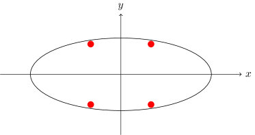
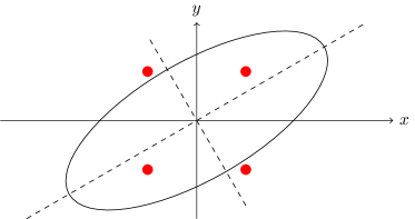
Figure 1: Illustration of feasible sets in (Left) the QCQP Class III and (Right) sequence design. Red dots represent the possible binary vectors. Black ellipses represent the bounds of inequality constraints.

In summary, binary sequences $\tilde{\mathbf{s}}$ resulting from $\widehat{\mathbf{S}}$ via randomized projection and binary quantization may not be feasible to the inequality constraint, i.e., $\left\|\mathcal{F}_{I}^{H}\tilde{\mathbf{s}}\right\|_{2}^{2}\geq\alpha$. Analyzing the performance of $\tilde{\mathbf{s}}$ consists of evaluating the feasibility probability and approximation ratio: the former describes how often $\tilde{\mathbf{s}}$ satisfies the inequality constraints and the latter measures how good $\tilde{\mathbf{s}}$ is provided that it is feasible.

Intuitively, the feasibility probability of $\tilde{\mathbf{s}}$ highly depends on $\alpha$ and the rank of $\mathcal{F}_{I}$, which is also the width of the interferer band. As can be seen in Figure 1, decreasing $\alpha$ shrinks the ellipsoid defined by the inequality constraints and therefore fewer binary sequences are contained in the ellipsoid, which causes a reduced feasibility probability. Furthermore, a wider interferer band put more strict constraints on the sequences, which makes it harder for the sequences to to be feasible. These can be shown in the following theorem, proven in Appendix A.

Theorem 1

Assume that $\widehat{\mathbf{S}}$ is a solution for the SDP relaxation (25) and $\tilde{\mathbf{s}}$ is a binary vector obtained via randomized projection and binary quantization from $\mathbf{S}$. Define the ratio

$$\beta=\frac{\operatorname{Trace}\left(\mathcal{F}_{I}\mathcal{F}_{I}^{H}\arcsin\widehat{\mathbf{S}}\right)}{\operatorname{Trace}\left(\mathcal{F}_{I}\mathcal{F}_{I}^{H}\widehat{\mathbf{S}}\right)}.$$ (26)

Then, we have

$$\mathbb{P}\left\{\|\mathcal{F}_{I}^{H}\tilde{\mathbf{s}}\|_{2}^{2}\geq\frac{1}{\pi}\left(\beta+1\right)\alpha\right\}\leq\exp\left(-C\frac{\alpha^{2}}{K^{2}}\right).$$ (27)

where $C$ is a constant and $K$ is the column number of $\mathcal{F}_{I}$.

It is worthing noting that the ratio $\beta$ depends on the particular solution $\widehat{\mathbf{S}}$. Furthermore, it is impossible to obtain a upper bound for $\beta$. To see this, consider the case when all columns of $\widehat{\mathbf{S}}$ lie in the null space of $\mathcal{F}_{I}$, which would cause $\operatorname{Trace}\left(\mathcal{F}_{I}^{H}\mathcal{F}_{I}\mathbf{S}\right)=0$. The ratio $\beta$ will be infinite even if $\operatorname{Trace}\left(\mathcal{F}_{I}^{H}\mathcal{F}_{I}\arcsin\widehat{\mathbf{S}}\right)$ is very small but not zero. We also evaluate this dependence numerically: Figure 2 shows the empirical probability of the ratio $\beta$ over randomly generated positive semidefinite matrices $\widehat{\mathbf{S}}$ for several choices of sequence design problems. Virtually all instances of the ratio $\beta$ are below $\pi-1\approx 2.14$. When this bound on $\beta$ holds, the result above is reduced to

$$\mathbb{P}\left\{\|\mathcal{F}_{I}^{H}\mathbf{s}\|_{2}^{2}\geq\alpha\right\}\leq\exp\left(-C\frac{\alpha^{2}}{K^{2}}\right).$$ (28)

Again, note that the reduction of the feasibility bound in (25) from $\alpha$ to $\alpha/2$ is necessary to obtain the result above, given the values of $\beta$ that are observed in practice.

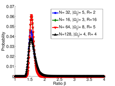
Figure 2: Empirical probability of the ratio $\beta$ between $\operatorname{Trace}\left(\mathcal{F}_{I}\mathcal{F}_{I}^{H}\arcsin\widehat{\mathbf{S}}\right)$ and $\operatorname{Trace}\left(\mathcal{F}_{I}\mathcal{F}_{I}^{H}\widehat{\mathbf{S}}\right)$ in different setting of sequence length $N$, interferer width $K$, and rank $R$ of $\widehat{\mathbf{S}}$.

Numerical simulations in the sequel serve as further validation of Theorem 1, and confirm the conclusion that the larger that $\alpha$ is, and the narrower that the interferer band is, the more likely that the sequence $\tilde{\mathbf{s}}$ will meet the interferer band power constraint. Additionally, Theorem 1 implies that it is necessary to generate a sufficiently large number of candidate sequences to meet the feasibility constraints, as described in Algorithm 1.

When $\tilde{\mathbf{s}}$ is feasible to all constraints, it is possible to calculate the approximation ratio. We claim the approximation ratio by the following conjecture. Such result matches the results of other QCQPs proved repeatedly in the literature, e.g., [40, Corollary 2.1] and [31, Proposition 1]. Though we have found a theoretical proof of the following statement elusive, we will verify the conjecture numerically in the sequel.

Conjecture 1

Consider a binary sequence $\tilde{\mathbf{s}}$ obtained via randomized projection and binary quantization from $\widehat{\mathbf{S}}$, which is the solution to (25). Given that $\tilde{\mathbf{s}}$ meets the inequality constraints, i.e., $\|\mathcal{F}_{I}\tilde{\mathbf{s}}\|_{2}^{2}\leq\alpha$, the approximation ratio

$$\gamma=\frac{\|\mathcal{F}_{M}\tilde{\mathbf{s}}\|_{2}^{2}}{\operatorname{Trace}\left(\mathcal{F}_{M}^{H}\mathcal{F}_{M}\widehat{\mathbf{S}}\right)}$$

satisfies $\gamma\geq\pi/2-1$.

Theorem 1 and Conjecture 1 together guarantee that it is possible to use the randomized projection and binary quantization to generate feasible binary sequences with high probability for which the message band power is no less than $\pi/2-1$ of the optimal power among arbitrary sequences. These two results are the theoretical foundation four our proposed binary sequence design method.

4.3 Sequence Selection

In Algorithm 1, the final sequence selection step not only excludes candidate sequences that fail the interferer constraints but also finds a sequence for which the value of the objective function is as close to the optimal sequence as possible. Intuitively, one would choose the feasible sequence that maximizes the objective function of (24), which corresponds to the sequence with maximal energy in the message band.

However, the sequence with the largest message power is not necessarily the best suited sequence for the problem of interest. As shown in Figure 3, the sequence selected according to the message band power maximization often has a large magnitude dynamic range (i.e., the ratio between the largest magnitude and smallest magnitude), in both the message band and the interferer band. Additionally, the sequence fails to attenuate the interferer with respect to the message since some magnitudes in the message band are smaller than some in the interferer band, which potentially does not allow for successful interference rejection.

To ensure the necessary attenuation, we propose the use of the interferer rejection ratio, which is defined as the ratio between the minimum magnitude of the spectrum in the message band and the maximum magnitude in the interferer band, i.e.,

$$\rho\left(\mathbf{s}\right):=\frac{\min\left|\mathcal{F}_{M}^{H}\mathbf{s}\right|}{\max\left|\mathcal{F}_{I}^{H}\mathbf{s}\right|},$$ (29)

where the absolute value is taken in an element-wise fashion and the minimum and maximum are evaluated over the entries of the corresponding vectors. We find that a sequence selection driven by this criterion provides more amenable spectra for the applications of interest, as shown in Figure 3. Furthermore, we also find in Figure 3 that the dynamic range of the spectra in the bands of interest is reduced as well.

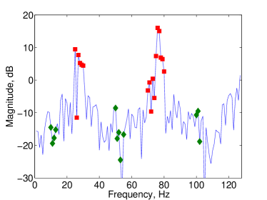
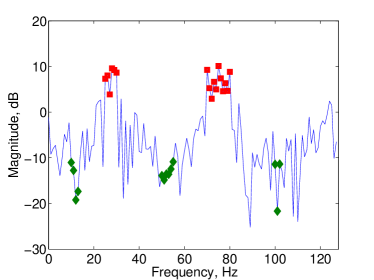
Figure 3: Spectra of example binary sequences that maximize (Left) the message power and (Right) the interferer rejection ratio (29). Green and red markers denote the interferer and message bands.

5 Numerical Experiments

To test our proposed binary sequence design algorithm, we present two groups of experiments: the first group provides experimental validation to the two theoretical results from Section 4; the second group studies the performance of the obtained sequences in comparison to existing approaches, including the modifications listed in Section 2 and the exhaustive search when feasible. In all experiments, the SDP optimization (24) is implemented using the CVX package [41, 42].

In the first experiment, we illustrate the probability that the candidate sequences $\tilde{\mathbf{s}}$, obtained according to Algorithm 1, satisfy the interferer constraint. We set the sequence length to $N=128$, and draw $L=10^{6}$ candidate sequences to evaluate the statistical behavior of the algorithm. Figure 4 shows the feasibility probability as a function of the interferer tolerance $\alpha\in[0.5,10]$ when the message and interferer bands include the frequencies $\Omega_{M}=\{25,26,\dots,30,40,41,\dots,45\}$ and $\Omega_{I}=\{10,11,\dots,15,50,51,\dots,55\}$, respectively, and the feasibility probability, when the message band is $\Omega_{M}=\{1,2,\dots,10,50,51,\dots,60\}$ and the interferer tolerance is $\alpha=3$, as a function of the interferer width $\left|\Omega_{I}\right|\in[1,20]$ such that the interferer band includes frequencies with indices $\Omega_{I}=\{20,21,\dots,20+\left|\Omega_{I}\right|\}$. Both validate the exponential relationships predicted by Theorem 1. The blue plots in the figures correspond to sequences drawn uniformly at random from ${\{-1,1\}}^{N}$. The random sequences have much lower probability to satisfy the interferer constraints than the candidate sequences. This indicates that it is beneficial to use the combination of an SDP relaxation and randomized projection to find the feasible sequence.

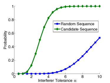
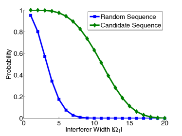
Figure 4: Probability of a candidate sequence satisfying the interferer constraint as a function of (Left) interferer tolerance and (Right) interferer bandwidth.

In the second experiment, we illustrate the distribution of the approximation ratio of the candidate sequence resulting from the randomized projection and binary quantization. The approximation ratio corresponds to the ratio of the values of the objective function $f(s)$ from (24) for the solution $\tilde{\mathbf{s}}$ obtained from Algorithm 1 to the objective function $f\left(S\right)$ from (25) for the solution $\widehat{\mathbf{S}}$. The setting is the same as in the previous experiments: $N=128$, $\Omega_{M}=\{25,26,\dots,30,40,41,\dots,45\}$, $\Omega_{I}=\{10,11,\dots,15,50,51,\dots,55\}$, $\alpha=5$ and $R=10^{6}$. We also compare to $R$ random binary sequences with entries drawn from a uniform Rademacher distribution. Figure 5 shows that all feasible sequences generated by Algorithm 1 have approximation ratio $\gamma\geq\pi/2-1$, which is marked by the red dotted line; the figure also shows that Algorithm 1 consistently outperforms random sequence designs, as expected from the spectral shaping. This numerically proves that the sequences obtained from Algorithm 1 meet the approximation ratio $\pi/2-1$, as proposed in Conjecture 1. Additionally, the results motivate the use of random projections rather than only eigendecomposition to obtain the candidate sequences, given that some feasible solutions are able to achieve a higher approximation ratio than the quantized principal eigenvector of $\widehat{\mathbf{S}}$, whose approximation ratio is marked by the black dashed line in Figure 5. These numerical results show that the candidate sequences obtained from Algorithm 1 have a high probability of satisfying the interferer constraints and large message band power, which we can interpret as successful spectrally shaped binary sequence design.

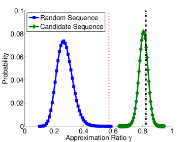
Figure 5: Distribution of approximation ratio $\gamma$ of candidate sequences that are feasible to the interferer constraints. The red dotted and black dashed lines represent the bound predicted by Conjecture 1 ($\gamma\geq\pi/2-1$) and the approximation ratio corresponding to the quantized principal eigenvector of $\widehat{\mathbf{S}}$, respectively.

In the third experiment, we compare the performance of the sequences obtained from Algorithm 1 versus the optimal sequences obtained by the exhaustive search in the term of message preservation and interferer rejection. By setting the sequence length $N=16$, we can feasibly perform an exhaustive search over all the $2^{16}=65536$ possible binary sequences. Both the message and interferer band contain only two frequency bins, and so there are $\binom{8}{2}\times\binom{6}{2}=420$ different choices to set the message and interferer band in the spectrum accordingly, given that message and interferer bands share no common frequency and the spectrum of a binary sequence is symmetric. Figure 6 shows the ratio of the performance metrics for the sequences obtained by Algorithm 1 over those for the optimal sequences from an exhaustive search as a function of the size of the random search size $R$ (i.e., the number of candidate sequences generated in Algorithm 1) after being normalized by the size of the exhaustive search space. We use three measures of performance averaged over all $420$ choices: the message band power, the interference rejection ratio (29) and the reciprocal message dynamic range, which is defined as

$$\chi(s)=\frac{\min\left|\mathcal{F}_{M}^{H}\mathbf{s}\right|}{\max\left|\mathcal{F}_{M}^{H}\mathbf{s}\right|},$$ (30)

to measure the dynamic range in message band. Noting that each of these metrics can be correspondingly used as the score function in the selection step of Algorithm 1. The message power of the sequences obtained from Algorithm 1 matches that obtained from exhaustive search, even if $R$, the random search size in Algorithm 1, is much smaller than the exhaustive search size. Though the proposed method could not find the sequence with largest interferer rejection ratio, it provides a good approximation with low complexity.

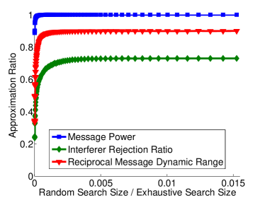
Figure 6: Average ratio of message power and interferer rejection ratio and reciprocal message dynamic range between the sequences obtained from Algorithm 1 and the optimal sequences from an exhaustive search.

In the fourth experiment, we compare the performance of the sequences obtained from Algorithm 1 versus both unimodular and binary sequences from SHAPE and LPNN algorithms (cf. Section 2) and versus the quantized principal eigenvector approach (cf. Section 3) over 100 randomly drawn message and interferer configurations. The sequence length and the message bandwidth are fixed to be $N=128$ with $|\Omega_{M}|=10$ and $|\Omega_{I}|$ varying between 1 and 10. The proposed algorithm chooses the best sequence from $R=10^{5}$ candidate sequences, while the maximum iteration for SHAPE and LPNN algorithms is $10000$. Figure 7 shows the average rejection ratio and computation time for all tested algorithms. Our proposed algorithm shows the ability to obtain a binary sequence with a clear distinction in the magnitude of the message and interferer bands. The performance of our proposed algorithm decreases as the interferer bandwidth becomes larger. Although it can be expected that the unimodular sequences obtained from both the SHAPE and the LPNN algorithms provide better interference rejection, surprisingly, our proposed method achieves performance similar to the unimodular sequences found by existing methods. Furthermore, our proposed method outperforms their binary-constrained versions, which is indicative of the difficulty of this more severely constrained problem. Note also that the quantized principal eigenvectors have much worse performance than the designed sequences, which is evidence of the benefit provided by the randomized projection search included in Algorithm 1.We finally note that the computation time for each algorithm is roughly constant over the interferer widths chosen: our proposed algorithm takes $356$ seconds on average while both versions of SHAPE take $0.5$ seconds on average, and the two versions of LPNN take $606$ and $181$ seconds on average, respectively.

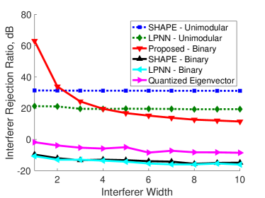
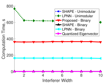
Figure 7: Average interferer rejection ratio (Left) and computation time (Right) of SHAPE and LPNN for unimodular sequence and binary sequence and Algorithm 1 for binary sequence.

6 Conclusion

In this paper, we propose an algorithm to design a spectrally shaped binary sequence that provides a passband and a notch for a pair of pre-determined message and interferer bands, respectively. We first pose the sequence design problem as a QCQP problem, and combine it with a randomized projection of the solution of an SDP relaxation (a common convex relaxation) to obtain an approximation to the optimal sequence in a statistical sense. The candidate sequences obtained by this method are shown to satisfy the interferer constraints with a probability that depends on the interferer tolerance and the interferer bandwidth. We numerically show that the candidate sequences are better approximations (in terms of the objective function value) than sequences obtained by quantizing the principal eigenvector and than randomly generated binary sequences. Our method also outperforms existing approaches for unimodular sequence design that are modified to meet the required binary quantization constraint. Our experiments show that for small sequence lengths the proposed method is able to obtain the same optimal sequences as the exhaustive search at a fraction of the search cost, which shows promise for the use of our randomized method in spectrally shaped binary sequence design featuring larger length.

Many questions remain open both on the analysis and possible refinements of our algorithm. For example, the binary constraint places a significant limitation on the sequence design space. More flexible quantization schemes that allow for multiple levels in the values of the sequence may improve the performance of our method while still allowing for a feasible implementation. Furthermore, one could consider changes to the objective function and the constraints (e.g., switching the two) and to the selection score function in order to make the sequences obtained more relevant to other types of applications. Possible examples include considering the dynamic range of the message and interferer spectra or the allocation of transmission power to different parts of the spectrum.

Appendix A Proof of Theorem 1

We will use the following results in our proof.

Theorem 2 (McDiarmid’s Inequality [43])

Let $X={[X_{1},X_{2},\dots,X_{N}]}^{T}$ be a family of random variables with $X_{i}$ taking values in a set $\Lambda_{i}$ for each $i\in\mathcal{I}=\{1,2,\dots,N\}$. Assume the function $g:\prod_{i\in\mathcal{I}}\Lambda_{i}\rightarrow\mathbb{R}$ satisfies $|g\left(\mathbf{x}\right)-g\left(\bar{\mathbf{x}}\right)|\leq c_{n}$ whenever $\mathbf{x},\bar{\mathbf{x}}\in\prod_{i\in\mathcal{I}}\Lambda_{i}$ differ only in their $n^{\textrm{th}}$ entries for some $n\in\mathcal{I}$. For any $\zeta>0$, we have

$$\mathbb{P}\left\{g(X)>\mathbb{E}\left(g(X)\right)+\zeta\right\}\leq\exp\left(-\frac{2\zeta^{2}}{\sum_{i\in\mathcal{I}}c_{i}^{2}}\right).$$ (31)

To use Theorem 2 to prove Theorem 1, we need to present some additional results.

Lemma 1 ([27, Lemma 3.2])

If $s$ is a binary vector obtained via randomized projection and binary quantization from $S$, then for any indices $i,j\in\mathcal{I}$,

$$\mathbb{P}\left\{s_{i}\neq s_{j}\right\}=\frac{1}{\pi}\arccos\left(\frac{S_{i,j}}{\sqrt{S_{i,i}S_{j,j}}}\right).$$ (32)

This lemma provides an important connection between the original binary sequence design and its SDP relaxation, and allows us to prove the following result, which we have found in the literature without proof.

Lemma 2

If $\mathbf{s}$ is a binary vector obtained via randomized projection and binary quantization from $\mathbf{S}$, then

$$\mathbb{E}\left(\mathbf{s}_{i}\mathbf{s}_{j}\right)=\frac{2}{\pi}\arcsin\mathbf{S}_{i,j},$$ (33)

for any indices $i,j\in\mathcal{I}$.

Proof. Since $\mathbf{S}$ is a solution for the SDP relaxation (25), $\mathbf{S}_{i,i}=1$ for each $i\in\mathcal{I}$, and so $\mathbb{E}\left(\mathbf{s}_{i}^{2}\right)=1=\frac{2}{\pi}\arcsin\mathbf{S}_{i,i}$. When $i\neq j$,

$$\mathbb{E}\left(\mathbf{s}_{i}\mathbf{s}_{j}\right) =1-2\mathbb{P}\left\{\mathbf{s}_{i}\neq\mathbf{s}_{j}\right\}=\frac{2}{\pi}\left(\frac{\pi}{2}-\arccos\mathbf{S}_{i,j}\right)=\frac{2}{\pi}\arcsin\mathbf{S}_{i,j},$$ (34)

where the second equality is due to Lemma 1 $\square$

To use McDiarmid’s Inequality, we need to prove the following conditions for binary sequences.

Lemma 3

If $\mathbf{s}$ is a binary vector obtained via randomized projection and binary quantization from $S$, then $\left|\left\|\mathcal{F}_{I}^{H}\mathbf{s}\right\|_{2}^{2}-\left\|\mathcal{F}_{I}^{H}\bar{\mathbf{s}}\right\|_{2}^{2}\right|\leq 4|\Omega_{I}|$ whenever $\mathbf{s},\bar{\mathbf{s}}\in{\{-1,1\}}^{N}$ differ only in the $n^{\mathrm{th}}$ entries for any $n\in\mathcal{I}$.

Proof. We can express the entries of $\mathcal{F}_{I}$ as $a_{k,i}=\frac{1}{\sqrt{N}}e^{\left(\jmath 2\pi(k-1)(i-1)/N\right)}$ ($k\in\Omega_{I}$, $i\in\mathcal{I}$). Since $\mathcal{F}_{I}$ is a submatrix of the Fourier orthonormal basis matrix, $\sum_{i\in\mathcal{I}}|a_{k,i}|^{2}=1$. Additionally,

$$\left\|\mathcal{F}_{I}^{H}\mathbf{s}\right\|_{2}^{2} =\operatorname{Trace}\left(\mathcal{F}_{I}\mathcal{F}_{I}^{H}\mathbf{s}\mathbf{s}^{T}\right)=\sum_{i\in\mathcal{I}}\sum_{j\in\mathcal{I}}\sum_{k\in\Omega_{I}}a_{k,i}^{*}a_{k,j}s_{i}s_{j}$$

$$=\sum_{i\neq n}\sum_{j\neq n}\sum_{k\in\Omega_{I}}a_{k,i}^{*}a_{k,j}s_{i}s_{j}+\sum_{i\neq n}\sum_{k\in\Omega_{I}}a_{k,i}^{*}a_{k,n}s_{i}s_{n}+\sum_{j\neq n}\sum_{k\in\Omega_{I}}a_{k,n}^{*}a_{k,j}s_{n}s_{j}+\sum_{k\in\Omega_{I}}a_{k,n}^{*}a_{k,n}s_{n}^{2}.$$ (35)

Since $\mathbf{s},\bar{\mathbf{s}}\in{\{-1,1\}}^{N}$ differ only in the $n^{\text{th}}$ entries, $s_{i}=\bar{s}_{i}$ if $i\neq n$ and $s_{n}^{2}=\bar{s}_{n}^{2}=1$. The first and fourth terms in the right hand side of (A) for $\left\|\mathcal{F}_{I}^{H}\mathbf{s}\right\|_{2}^{2}$ and $\left\|\mathcal{F}_{I}^{H}\bar{\mathbf{s}}\right\|_{2}^{2}$ are the same. Therefore,

$$\left|\left\|\mathcal{F}_{I}^{H}\mathbf{s}\right\|_{2}^{2}-\left\|\mathcal{F}_{I}^{H}\bar{\mathbf{s}}\right\|_{2}^{2}\right| =\left|\sum_{i\neq n}\sum_{k\in\Omega_{I}}a_{k,i}^{*}a_{k,n}s_{i}\left(s_{n}-\bar{s}_{n}\right)+\sum_{j\neq n}\sum_{k\in\Omega_{I}}a_{k,n}^{*}a_{k,j}s_{j}\left(s_{n}-\bar{s}_{n}\right)\right|$$

$$\leq 2\left|\sum_{i\neq n}\sum_{k\in\Omega_{I}}a_{k,i}^{*}a_{k,n}s_{i}\right|\left|s_{n}-\bar{s}_{n}\right|\leq 4\sqrt{\sum_{k\in\Omega_{I}}|a_{k,n}|^{2}\sum_{k\in\Omega_{I}}\left|\sum_{i\neq n}a_{k,i}^{*}s_{i}\right|^{2}}$$

$$\leq 4\sqrt{\sum_{k\in\Omega_{I}}|a_{k,n}|^{2}}\sqrt{\sum_{k\in\Omega_{I}}\sum_{i\neq n}|a_{k,i}|^{2}\sum_{i\neq n}s_{i}^{2}}\leq 4\sqrt{\frac{|\Omega_{I}|}{N}}\sqrt{|\Omega_{I}|\frac{N-1}{N}(N-1)}$$

$$\leq 4|\Omega_{I}|,$$ (36)

where the second and third inequalities result from Cauchy-Schwarz inequality. $\square$

Now, we are ready to prove Theorem 1. From (33), we have

$$\mathbb{E}\left(\left\|\mathcal{F}_{I}^{H}\mathbf{s}\right\|_{2}^{2}\right) =\mathbb{E}\left(\mathbf{s}^{T}\mathcal{F}_{I}\mathcal{F}_{I}^{H}\mathbf{s}\right)=\mathbb{E}\left(\operatorname{Trace}\left(\mathcal{F}_{I}\mathcal{F}_{I}^{H}\mathbf{s}\mathbf{s}^{T}\right)\right)=\operatorname{Trace}\left(\mathcal{F}_{I}\mathcal{F}_{I}\mathbb{E}\left(\mathbf{s}\mathbf{s}^{T}\right)\right)=\frac{2}{\pi}\operatorname{Trace}\left(\mathcal{F}_{I}^{H}\mathcal{F}_{I}\arcsin\mathbf{S}\right)$$

$$\leq\frac{1}{\pi}\beta\alpha,$$ (37)

where the last inequality results from (26) and the constraint in (25).

By picking $\zeta=\frac{1}{\pi}\alpha>0$ and applying McDiarmid’s inequality for $g(\mathbf{s})=\left\|\mathcal{F}_{I}\mathbf{s}\right\|_{2}^{2}$ with Lemma 3 and (37), we finally obtain

$$\mathbb{P}\left\{\left\|\mathcal{F}_{I}\mathbf{s}\right\|_{2}^{2}\geq\frac{1}{\pi}\left(\beta+1\right)\alpha\right\} =\mathbb{P}\left\{g(\mathbf{s})\geq\mathbb{E}\left(g(\mathbf{s})\right)+\frac{1}{\pi}\alpha\right\}\leq\exp\left(-\frac{2{\left(\frac{1}{\pi}\alpha\right)}^{2}}{N{\left(4|\Omega_{I}|\right)}^{2}}\right)\leq\exp\left(-\frac{1}{8N\pi^{2}}\frac{\alpha^{2}}{|\Omega_{I}|^{2}}\right).$$

This completes the proof of Theorem 1.

References

- [1] D. Mo and M. F. Duarte, “Design of spectrally shaped binary sequences via randomized convex relaxations,” in Asilomar Conf. Signals, Syst. and Comp., Pacific Grove, CA, Nov. 2015, pp. 164–168.
- [2] J. Salzman, D. Akamine, and R. Lefevre, “Optimal waveforms and processing for sparse frequency UWB operation,” in Proc. IEEE Radar Conf., Atlanta, GA, May 2001, pp. 105–110.
- [3] W. Rowe, P. Stoica, and J. Li, “Spectrally constrained waveform design,” IEEE Signal Process. Mag., vol. 31, no. 3, pp. 157–162, May 2014.
- [4] A. Aubry, A. D. Maio, M. Piezzo, and A. Farina, “Radar waveform design in a spectrally crowded environment via nonconvex quadratic optimization,” IEEE Trans. Aerosp. Electron. Syst., vol. 50, no. 2, pp. 1138–1152, Apr. 2014.
- [5] A. Aubry, A. D. Maio, Y. Huang, M. Piezzo, and A. Farina, “A new radar waveform design algorithm with improved feasibility for spectral coexistence,” IEEE Trans. Aerosp. Electron. Syst., vol. 51, no. 2, pp. 1029–1038, Apr. 2015.
- [6] J. N. Laska, S. Kirolos, M. F. Duarte, T. S. Ragheb, R. G. Baraniuk, and Y. Massoud, “Theory and implementation of an analog-to-information converter using random demodulation,” in IEEE Int. Symp. Circuits Syst. (ISCAS), New Orleans, LA, May 2007, pp. 1959–1962.
- [7] M. Mishali and Y. C. Eldar, “Blind multiband signal reconstruction: Compressed sensing for analog signals,” IEEE Trans. Signal Process., vol. 57, no. 3, pp. 993–1009, Mar. 2009.
- [8] J. A. Tropp, J. N. Laska, M. F. Duarte, J. K. Romberg, and R. G. Baraniuk, “Beyond Nyquist: Efficient sampling of sparse bandlimited signals,” IEEE Trans. Inf. Theory, vol. 56, no. 1, pp. 520–544, Jan 2010.
- [9] T. C. Clancy and D. Walker, “Spectrum shaping for interference management in cognitive radio networks,” in SDR Forum Tech. Conf., Denver, USA, Nov. 2006.
- [10] J. Li and P. Stoica, MIMO Radar Signal Processing. New York, NJ: Wiley-IEEE Press, Oct. 2008.
- [11] K. Zhao, J. Liang, J. Karlsson, and J. Li, “Enhanced multistatic active sonar signal processing,” in IEEE Int. Conf. Acoust, Speech and Signal Process. (ICASSP),, Vancouver, BC, Canada, May 2013, pp. 3861 – 3865.
- [12] J. Liang, L. Xu, J. Li, and P. Stoica, “On designing the transmission and reception of multistatic continuous active sonar systems,” IEEE Trans. Aerosp. Electron. Syst., vol. 50, no. 1, pp. 285–299, Jan. 2014.
- [13] H. He, J. Li, and P. Stoica, Waveform Design for Active Sensing Systems: A Computational Approach. Cambridge, UK: Cambridge University Press, Jun. 2012.
- [14] P. Stoica, H. He, and J. Li, “New algorithms for designing unimodular sequences with good correlation properties,” IEEE Trans. Signal Process., vol. 57, no. 4, pp. 1415–1425, Apr. 2009.
- [15] ——, “On designing sequences with impulse-like periodic correlation,” IEEE Signal Process. Lett., vol. 16, no. 8, pp. 703–706, Aug. 2009.
- [16] J. Song, P. Babu, and D. P. Palomar, “Optimization methods for designing sequences with low autocorrelation sidelobes,” IEEE Trans. Signal Process., vol. 63, no. 15, pp. 3998–4009, Aug. 2015.
- [17] ——, “Sequence design to minimize the weighted integrated and peak sidelobe levels,” IEEE Trans. Signal Proc., vol. 64, no. 8, pp. 2051–2064, April 2016.
- [18] M. A. Kerahroodi, A. Aubry, A. D. Maio, M. M. Naghsh, and M. Modarres-Hashemi, “A coordinate-descent framework to design low psl/isl sequences,” IEEE Trans. Signal Proc., vol. 65, no. 22, pp. 5942–5956, Nov. 2017.
- [19] L. Zhao, J. Song, P. Babu, and D. P. Palomar, “A unified framework for low autocorrelation sequence design via majorization–minimization,” IEEE Trans. Signal Proc., vol. 65, no. 2, pp. 438–453, Jan. 2017.
- [20] Y. Li and S. A. Vorobyov, “Fast algorithms for designing unimodular waveform(s) with good correlation properties,” IEEE Trans. Signal Proc., vol. 66, no. 5, pp. 1197–1212, March 2018.
- [21] J. Liang, H. C. So, J. Li, and A. Farina, “Unimodular sequence design based on alternating direction method of multipliers,” IEEE Trans. Signal Proc., vol. 64, no. 20, pp. 5367–5381, Oct. 2016.
- [22] J. Liang, H. C. So, C. S. Leung, J. Li, and A. Farina, “Waveform design with unit modulus and spectral shape constraints via lagrange programming neural network,” IEEE J. Sel. Topics Signal Process., vol. 9, no. 8, pp. 1377–1386, Dec. 2015.
- [23] S. Zhang and A. G. Constantinides, “Lagrange programming neural networks,” IEEE Trans. Circuits. Syst II, Analog Digit. Signal Process., vol. 39, no. 7, pp. 441–452, Jul. 1992.
- [24] Z.-Q. Luo, N. D. Sidiropoulos, P. Tseng, and S. Zhang, “Approximation bounds for quadratic optimization with homgeneous quadratic constraints,” SIAM J. Optim., vol. 18, no. 1, pp. 1–28, Feb. 2007.
- [25] N. Z. Shor, “Quadratic optimization problems,” Soviet J. Comput. Systems Sci., vol. 25, no. 6, pp. 1–11, 1987.
- [26] L. Lovász and A. Schrijver, “Cones of matrices and set-functions and 0-1 optimization,” SIAM J. Optim., vol. 1, no. 2, pp. 166–190, Oct. 1991.
- [27] M. X. Goemans and D. P. Williamson, “Improved approximation algorithms for maximum cut and satisfiability problems using semidefinite programming,” J. ACM, vol. 42, no. 6, pp. 1115–1145, Nov. 1995.
- [28] M. Fu, Z.-Q. Luo, and Y. Ye, “Approximation algorithms for quadratic programming,” J. Comb. Optim., vol. 2, no. 1, pp. 29–50, Mar. 1998.
- [29] Y. Nesterov, “Semidefinite relaxation and nonconvex quadratic optimization,” Optim. Methods and Softw., vol. 9, no. 1-3, pp. 141–160, 1998.
- [30] Y. Ye, “Approximating global quadratic optimization with convex quadratic constraints,” J. Global Optim., vol. 15, no. 1, pp. 1–17, Jan. 1999.
- [31] ——, “Approximating quadratic programming with bound and quadratic constrains,” Math. Program., vol. 84, no. 2, pp. 219–226, Feb. 1999.
- [32] A. Nemirovski, C. Roos, and T. Terlaky, “On maximization of quadratic form over intersection of ellipsoids with common center,” Math. Program., vol. 86, no. 3, pp. 463–473, 1999.
- [33] S. Zhang, “Quadratic maximization and semidefinite relaxation,” Math. Program., vol. 87, no. 3, pp. 453–465, May 2000.
- [34] A. D. Maio, S. D. Nicola, Y. Huang, S. Zhang, and A. Farina, “Code design to optimize radar detection performance under accuracy and similarity constraints,” IEEE Trans. Signal Proc., vol. 56, no. 11, pp. 5618–5629, Nov. 2008.
- [35] A. D. Maio, S. D. Nicola, Y. Huang, Z.-Q. Luo, and S. Zhang, “Design of phase codes for radar performance optimization with a similarity constraint,” IEEE Trans. Signal Proc., vol. 57, no. 2, pp. 610–621, Feb. 2009.
- [36] A. D. Maio, Y. Huang, M. Piezzo, S. Zhang, and A. Farina, “Design of optimized radar codes with a peak to average power ratio constraint,” IEEE Trans. Signal Proc., vol. 59, no. 6, pp. 2683–2697, Jun. 2011.
- [37] G. Cui, H. Li, and M. Rangaswamy, “MIMO radar waveform design with constant modulus and similarity constraints,” IEEE Trans. Signal Proc., vol. 62, no. 2, pp. 343–353, Jan. 2014.
- [38] A. Aubry, V. Carotenuto, and A. D. Maio, “Forcing multiple spectral compatibility constraints in radar waveforms,” IEEE Signal Process. Lett., vol. 23, no. 4, pp. 483–487, Apr. 2016.
- [39] F. A. Potra and S. J. Wright, “Interior-point methods,” J. Comput. Appl. Math., vol. 124, no. 1-2, pp. 281–302, Dec. 2000.
- [40] Y. Nesterov, “Global quadratic optimization via conic relaxation,” in Handbook of Semidefinite Programming, Theory, Algorithms, and Applications, H. Wolkowicz, R. Saigal, and L. Vandenberghe, Eds. Springer, Feb. 2000, ch. 13, pp. 363–387.
- [41] M. Grant and S. Boyd, “Graph implementations for nonsmooth convex programs,” in Recent Advances in Learning and Control, ser. Lecture Notes in Control and Information Sciences, V. Blondel, S. Boyd, and H. Kimura, Eds. London: Springer London, 2008, pp. 95–110.
- [42] ——, “CVX: Matlab software for disciplined convex programming, version 2.1,” Available at http://cvxr.com/cvx, Mar. 2014.
- [43] C. McDiarmid, “On the method of bounded differences,” in Surveys in Combinatorics, 1989: Invited Papers at the Twelfth British Combinatorial Conference, ser. London Mathematical Society Lecture Note Series, J. Siemons, Ed. Cambridge University Press, 1989, pp. 148–188.