Phase Spaces, Parity Operators, and the Born-Jordan Distribution

Abstract

Phase spaces as given by the Wigner distribution function provide a natural description of infinite-dimensional quantum systems. They are an important tool in quantum optics and have been widely applied in the context of time-frequency analysis and pseudo-differential operators. Phase-space distribution functions are usually specified via integral transformations or convolutions which can be averted and subsumed by (displaced) parity operators proposed in this work. Building on earlier work for Wigner distribution functions [A. Grossmann, Comm. Math. Phys. 48(3), 191 (1976)], parity operators give rise to a general class of distribution functions in the form of quantum-mechanical expectation values. This enables us to precisely characterize the mathematical existence of general phase-space distribution functions. We then relate these distribution functions to the so-called Cohen class [L. Cohen, J. Math. Phys. 7(5), 781 (1966)] and recover various quantization schemes and distribution functions from the literature. The parity-operator approach is also applied to the Born-Jordan distribution which originates from the Born-Jordan quantization [M. Born, P. Jordan, Z. Phys. 34(1), 858 (1925)]. The corresponding parity operator is written as a weighted average of both displacements and squeezing operators and we determine its generalized spectral decomposition. This leads to an efficient computation of the Born-Jordan parity operator in the number-state basis and example quantum states reveal unique features of the Born-Jordan distribution.

1 Introduction

There are at least three logically independent descriptions of quantum mechanics: the Hilbert-space formalism cohen1991quantum , the path-integral method feynman2005 , and the phase-space approach such as given by the Wigner function carruthers1983 ; hillery1997 ; kim1991 ; lee1995 ; gadella1995 ; zachos2005 ; schroeck2013 ; SchleichBook ; Curtright-review . The phase-space formulation of quantum mechanics was initiated by Wigner in his ground-breaking work wigner1932 from 1932, in which the Wigner function of a spinless non-relativistic quantum particle was introduced as a quasi-probability distribution. The Wigner function can be used to express quantum-mechanical expectation values as classical phase-space averages. More than a decade later, Groenewold Gro46 and Moyal Moy49 formulated quantum mechanics as a statistical theory on a classical phase by mapping a quantum state to its Wigner function and they interpreted this correspondence as the inverse of the Weyl quantization Wey27 ; Weyl31 ; Weyl50 .

Coherent states have become a natural way to extend phase spaces to more general physical systems 1bayen1978 ; 2bayen1978 ; berezin74 ; berezin75 ; brif98 ; perelomov2012 ; gazeau ; ali2000 ; BERGERON2013 . In this regard, a new focus on phase-space representations for coupled, finite-dimensional quantum systems (as spin systems) rundle2021overview ; thesis ; DROPS ; koczor2016 ; koczor2017 ; koczor2018 ; KdG10 ; tilma2016 ; RTD17 ; LZG18 ; koczor2021 ; koczor2020 and their tomographic reconstructions rundle2017 ; leiner17 ; Leiner18 ; koczor2017 has emerged recently. A spherical phase-space representation of a single, finite-dimensional quantum system has been used to naturally recover the infinite-dimensional phase space in the large-spin limit koczor2017 ; koczor2018 . These spherical phase spaces have been defined in terms of quantum-mechanical expectation values of rotated parity operators tilma2016 ; RTD17 ; LZG18 ; koczor2017 ; koczor2018 ; thesis (as discussed below) in analogy with displaced reflection operators in flat phase spaces. But in the current work, we exclusively focus on the (usual) infinite-dimensional case which has Heisenberg-Weyl symmetries brif98 ; perelomov2012 ; gazeau ; LI94 . This case has been playing a crucial role in characterizing the quantum theory of light glauber2006nobel via coherent states and displacement operators Cahill68 ; cahill1969 ; agarwal1970 ; Agarwal68 and has also been widely used in the context of time-frequency analysis and pseudo-differential operators cohen1966generalized ; Cohen95 ; boggiatto2010time ; boggiatto2010weighted ; boggiatto2013hudson ; bornjordan ; thewignertransform ; groechenig2001foundations . Many particular phase spaces have been unified under the concept of the so-called Cohen class cohen1966generalized ; Cohen95 ; thewignertransform (see Definition 2 below), i.e. all functions which are related to the Wigner function via a convolution with a distribution (which is also known as the Cohen kernel).

Phase-space distribution functions are mostly described by one of the following three forms: (a) convolved derivatives of the Wigner function bornjordan ; thewignertransform , (b) integral transformations of a pure state (i.e. a rapidly decaying, complex-valued function) wigner1932 ; cohen1966generalized ; Cohen95 ; boggiatto2010time ; boggiatto2010weighted ; boggiatto2013hudson ; bornjordan ; thewignertransform , or (c) as integral transformations of quantum-mechanical expectation values Cahill68 ; cahill1969 ; agarwal1970 ; Agarwal68 . Also, Wigner functions (and the corresponding Weyl quantization) are usually described by integral transformations. But the seminal work of Grossmann Grossmann1976 ; thewignertransform (refer also to Royer77 ) allowed for a direct interpretation of the Wigner function as a quantum-mechanical expectation value of a displaced parity operator $\mathrm{\Pi}$ (which reflects coordinates $\mathrm{\Pi}\,\psi(x)=\psi(-x)$ of a quantum state $\psi$). In particular, Grossmann Grossmann1976 showed that the Weyl quantization of the delta distribution determines the parity operator $\mathrm{\Pi}$. This approach has been widely adopted dahl1982group ; dahl1988morse ; LIParity ; bishop1994 ; gadella1995 ; Royer1989 ; Royer96 ; chountasis1999 .

However, parity operators similar to the one by Grossmann and Royer Grossmann1976 ; Royer77 ; thewignertransform have still been lacking for general phase-space distribution functions. (Note that such a form appeared implicitly for $s$-parametrized distribution functions in moya1993 ; cahill1969 .) In the current work, we generalize the previously discussed parity operator $\mathrm{\Pi}$ Grossmann1976 ; Royer77 ; thewignertransform for the Wigner function by introducing a family of parity operators $\mathrm{\Pi}_{\theta}$ (refer to Definition 3) which is parametrized by a function or distribution $\theta$. This enables us to specify general phase-space distribution functions in the form of quantum-mechanical expectation values (refer to Definition 4) as

$$F_{\rho}(\mathrm{\Omega},\theta):=(\pi\hbar)^{-1}\,\mathrm{Tr}\,[\,\rho\,\mathcal{D}(\mathrm{\Omega})\mathrm{\Pi}_{\theta}\mathcal{D}^{\dagger}(\mathrm{\Omega})].$$

We will refer to the above operator $\mathrm{\Pi}_{\theta}$ as a parity operator following the lead of Grossmann and Royer Grossmann1976 ; Royer77 and given its resemblance and close analogy to the reflection operator $\mathrm{\Pi}$ discussed in prior work bishop1994 ; tilma2016 ; RTD17 ; LZG18 ; koczor2017 ; koczor2018 ; thesis . Here, $\mathcal{D}(\mathrm{\Omega})$ denotes the displacement operator and $\Omega$ describes suitable phase-space coordinates (see Sec. 3.1). (Recall that $\hbar=h/(2\pi)$ is defined as the Planck constant $h$ divided by $2\pi$.) The quantum-mechanical expectation values in the preceding equation give rise to a rich family of phase-space distribution functions $F_{\rho}(\mathrm{\Omega},\theta)$ which represent arbitrary (mixed) quantum states as given by their density operator $\rho$. In particular, this family of phase-space representations contains all elements from the (above mentioned) Cohen class and naturally includes the pivotal Husimi Q and Born-Jordan distribution functions.

We would like to emphasize that our approach to phase-space representations averts the use of integral transformations, Fourier transforms, or convolutions as these are subsumed in the parity operator $\mathrm{\Pi}_{\theta}$ which is independent of the phase-space coordinate $\Omega$. Although our definition also relies on an integral transformation given by a Fourier transform, it is only applied once and is completely absorbed into the definition of a parity operator thereby avoiding redundant applications of Fourier transforms. This leads to significant advantages as compared to earlier approaches:

• conceptual advantages (see also moya1993 ; KdG10 ; tilma2016 ; koczor2017 ; RTD17 ):

  • The phase-space distribution function is given as a quantum-mechanical expectation value. And this form nicely fits with the experimental reconstruction of quantum states Banaszek99 ; heiss2000discrete ; Bertet02 ; deleglise2008 ; rundle2017 ; koczor2017 ; Lutterbach97 .

  • All the complexity from integral transformations (etc.) is condensed into the parity operator $\mathrm{\Pi}_{\theta}$.

  • The dependence on the distribution $\theta$ and the particular phase space is separated from the displacement $\mathcal{D}(\mathrm{\Omega})$.

• computational advantages:

  • The repeated and expensive computation of integral transformations (etc.) in earlier approaches is avoided as $\mathrm{\Pi}_{\theta}$ has to be determined only once. Also, the effect of the displacement $\mathcal{D}(\mathrm{\Omega})$ is relatively easy to calculate.

In this regard, the current work can also be seen as a continuation of koczor2017 where the parity-operator approach has been emphasized, but mostly for finite-dimensional quantum systems. Moreover, we connect results from quantum optics cahill1969 ; Cahill68 ; glauber2006nobel ; leonhardt97 , quantum-harmonic analysis werner1984 ; thewignertransform ; bornjordan ; daubechies1980distributions ; daubechies1980coherent ; daubechies1980I ; daubechies1983II ; keyl2016 ; cohen2012weyl , and group-theoretical approaches brif98 ; perelomov2012 ; gazeau ; LI94 . It is also our aim to narrow the gap between different communities where phase-space methods have been successfully applied.

On the other hand, a major contribution of our work is the analysis of existence properties of generalized phase-space distributions and their parity operators. While the Wigner function has been known to exist for the general class of tempered distributions (a class of generalized functions that includes the pivotal $L^{2}$ space), we further illuminate which classes of Cohen kernels yield well-defined generalized phase-space distribution functions. Such existence questions are fully absorbed into the parity operators and precise conditions are used to guarantee their mathematical existence.

Similarly as the parity operator $\mathrm{\Pi}$ (which is the Weyl quantization of the delta distribution), we show that its generalizations $\mathrm{\Pi}_{\theta}$ are Weyl quantizations of the corresponding Cohen kernel $\theta$ (refer to Sec. 4.3 for the precise definition of the Weyl quantization used in this work). We discuss how these general results reduce to well-known special cases and discuss properties of phase-space distributions in relation to their parity operators $\mathrm{\Pi}_{\theta}$. In particular, we consider the class of $s$-parametrized distribution functions glauber2006nobel ; cahill1969 ; Cahill68 ; moya1993 , which include the Wigner, Glauber P, and Husimi Q functions, as well as the $\tau$-parametrized family, which has been proposed in the context of time-frequency analysis and pseudo-differential operators bornjordan ; boggiatto2010time ; boggiatto2010weighted ; boggiatto2013hudson . We derive spectral decompositions of parity operators for all of these phase-space families, including the Born-Jordan distribution. Relations of the form $\mathrm{\Pi}_{\theta}=A_{\theta}\circ\mathrm{\Pi}$ motivate the name “parity operator” as they are in fact compositions of the usual parity operator $\mathrm{\Pi}$ followed by some operator $A_{\theta}$ that usually corresponds to a geometric or physical operation (which commutes with $\mathrm{\Pi}$). In particular, $A_{\theta}$ is a squeezing operator for the $\tau$-parametrized family and corresponds to photon loss for the $s$-parametrized family (assuming $s<0$). This structure of the parity operators $\mathrm{\Pi}_{\theta}$ connects phase spaces to elementary geometric and physical operations (such as reflection, squeezing operators, photon loss) and these concepts are central to applications: the squeezing operator models a non-linear optical process which generates non-classical states of light in quantum optics mandel1995 ; glauber2007 ; leonhardt97 . These squeezed states of light have been widely used in precision interferometry schnabel2017 ; Grangier87 ; Xiao87 ; McKenzie2002 or for enhancing the performance of imaging lugiato2002 ; treps2003 , and the gravitational-wave detector GEO600 has been operating with squeezed light since 2010 abadie2011 ; grote2013 .

The Born-Jordan distribution and its parity operator constitute a most peculiar instance among the phase-space approaches. This distribution function has convenient properties, e.g., it satisfies the marginal conditions and therefore allows for a probabilistic interpretation bornjordan . The Born-Jordan distribution is however difficult to compute. But most importantly, the Born-Jordan distribution and its corresponding quantization scheme have a fundamental importance in quantum mechanics. In particular, there have been several attempts in the literature to find the “right” quantization rule for observables using either algebraic or analytical techniques. In a recent paper FPBJ , one of us has analyzed the Heisenberg and Schrödinger pictures of quantum mechanics, and it is shown that the equivalence of both theories requires that one must use the Born–Jordan quantization rule (as proposed by Born and Jordan born25 )

$$\text{(BJ)}\quad x^{m}p^{\ell}\mapsto\frac{1}{m{+}1}\sum_{k=0}^{m}\hat{x}^{k}\hat{p}^{\ell}\hat{x}^{m-k},$$

instead of the Weyl rule

$$\text{(Weyl) }\quad x^{m}p^{\ell}\mapsto\frac{1}{2^{m}}\sum_{k=0}^{m}\binom{m}{k}\hat{x}^{k}\hat{p}^{\ell}\hat{x}^{m-k}$$

for monomial observables. The Born–Jordan and Weyl rules yield the same result only if $m<2$ or $\ell<2$; for instance in both cases the quantization of the product $xp$ is $\frac{1}{2}(\hat{x}\hat{p}+\hat{p}\hat{x})$. It is however easy to find physical examples which give different results. Consider for instance the square of the $z$ component of the angular momentum: it is given by

$$\ell_{z}^{2}=x^{2}p_{y}^{2}+y^{2}p_{x}^{2}-2xp_{x}yp_{y}$$

and its Weyl quantization is easily seen to be

$$\textup{Op}_{\textup{Weyl}}(\ell_{z}^{2})=\hat{x}_{x}^{2}\hat{p}_{y}^{2}+\hat{x}_{y}^{2}\hat{p}_{x}^{2}-\tfrac{1}{2}(\hat{x}_{x}\hat{p}_{x}{+}\hat{p}_{x}\hat{x}_{x})(\hat{x}_{y}\hat{p}_{y}{+}\hat{p}_{y}\hat{x}_{y})$$ (1)

while its Born–Jordan quantization is the different expression

$$\textup{Op}_{\textup{BJ}}(\ell_{z}^{2})=\hat{x}_{x}^{2}\hat{p}_{y}^{2}+\hat{x}_{y}^{2}\hat{p}_{x}^{2}-\tfrac{1}{2}(\hat{x}_{x}\hat{p}_{x}{+}\hat{p}_{x}\hat{x}_{x})(\hat{x}_{y}\hat{p}_{y}{+}\hat{p}_{y}\hat{x}_{y})-\tfrac{1}{6}\hbar^{2}.$$ (2)

(Recall that the operators $\hat{x}_{\eta}$ and $\hat{p}_{\kappa}$ satisfy the canonical commutation relations $[\hat{x}_{\eta},\hat{p}_{\kappa}]=i\hbar\delta_{\eta\kappa}$ using the spatial coordinates $\eta,\kappa\in\{x,y,z\}$ and the Kronecker delta $\delta_{\eta\kappa}$.) One of us has shown in dilemma that the use of (2) instead of (1) solves the so-called “angular momentum dilemma” dahl1 ; dahl2 . To a general observable $a(x,p)$, the Weyl rule associates the operator

$$\textup{Op}_{\textup{Weyl}}(a)=(2\pi\hbar)^{-1}\int\mathcal{F}_{\sigma}a(x,p)\mathcal{D}(x,p)\,\mathrm{d}x\,\mathrm{d}p$$

where $\mathcal{F}_{\sigma}a$ is the symplectic Fourier transform of $a$ and $\mathcal{D}(x,p)$ the displacement operator (see Sec. 3.1); in the Born–Jordan case this expression is replaced with

$$\textup{Op}_{\textup{BJ}}(a)=(2\pi\hbar)^{-1}\int\mathcal{F}_{\sigma}a(x,p)K_{\textup{BJ}}(x,p)\mathcal{D}(x,p)\,\mathrm{d}x\,\mathrm{d}p$$

where the filter function $K_{\textup{BJ}}(x,p)$ is given by

$$K_{\textup{BJ}}(x,p)=\mathrm{sinc}(\tfrac{px}{2\hbar})=\frac{\sin(\tfrac{px}{2\hbar})}{px/(2\hbar)}.$$

We obtain significant, new results for the case of Born-Jordan distributions and therefore substantially advance on previous characterizations. In particular, we derive its parity operator $\mathrm{\Pi}_{\textup{BJ}}$ in the form of a weighted average of geometric transformations

$$\mathrm{\Pi}_{\textup{BJ}}=\tfrac{1}{4\pi\hbar}\int\mathrm{sinc}(\tfrac{px}{2\hbar})\,\mathcal{D}(x,p)\,\mathrm{d}x\,\mathrm{d}p=[\,\tfrac{1}{4}\int_{-\infty}^{\infty}\,\mathrm{sech}(\tfrac{\xi}{2})S(\xi)\,\mathrm{d}\xi\,]\;\mathrm{\Pi},$$ (3)

where $\mathcal{D}(x,p)$ is the displacement operator and $S(\xi)$ is the squeezing operator (see Eq. (45) below) with a real squeezing parameter $\xi$. We have used the sinus cardinalis $\mathrm{sinc}(x):=\mathrm{sin}(x)/x$ and the hyperbolic secant $\mathrm{sech}(x):=1/\mathrm{cosh}(x)$ functions. The parity operator $\mathrm{\Pi}_{\textup{BJ}}$ in Eq. (3) decomposes into a product $\mathrm{\Pi}_{\theta}=A_{\theta}\circ\mathrm{\Pi}$ containing the usual reflection operator $\mathrm{\Pi}$. This is another example of the above-discussed motivation for our terminology of parity operators. We prove in Proposition 2 that $\mathrm{\Pi}_{\textup{BJ}}$ is a bounded operator on the Hilbert space of square-integrable functions and therefore gives rise to well-defined phase-space distribution functions of arbitrary quantum states. We derive a generalized spectral decomposition of this parity operator based on a continuous family of generalized eigenvectors that satisfy the following generalized eigenvalue equation for every real $E$ (see Theorem 5.3):

$$\mathrm{\Pi}_{\textup{BJ}}\,|\psi^{E}_{\pm}\rangle=\pm\pi/2\,\mathrm{sech}(\pi E)\,|\psi^{E}_{\pm}\rangle.$$

Facilitating a more efficient computation of the Born-Jordan distribution, we finally derive explicit matrix representations in the so-called Fock or number-state basis, which constitutes a natural representation for bosonic quantum systems such as in quantum optics mandel1995 ; glauber2007 ; leonhardt97 . Curiously, the parity operator $\mathrm{\Pi}_{\textup{BJ}}$ of the Born-Jordan distribution is not diagonal in the Fock basis as compared to the diagonal parity operators of $s$-parametrized phase spaces (cf.  koczor2017 ) that enable the experimental reconstruction of distribution functions from photon-count statistics deleglise2008 ; Lutterbach97 ; Bertet02 ; Banaszek99 in quantum optics. We calculate the matrix elements $[\mathrm{\Pi}_{\textup{BJ}}]_{mn}$ in the Fock or number-state basis and provide a convenient formula for a direct recursion, for which we conjecture that the matrix elements are completely determined by eight rational initial values. This recursion scheme has significant computational advantages for calculating Born-Jordan distribution functions as compared to previous approaches and allows for an efficient implementation. In particular, large matrix representations of the parity operator $\mathrm{\Pi}_{\textup{BJ}}$ can be well approximated using rank-9 matrices. We finally illustrate our results for simple quantum states by calculating their Born-Jordan distributions and comparing them to other phase-space representations. Let us summarize the main results of the current work:

• quantum-mechanical expectation values of the parity operators $\mathrm{\Pi}_{\theta}$ from Def. 3 define distribution functions (see Def. 4) and form the Cohen class (Theorem 4.1);

• existence properties of parity operators and generalized phase-space functions are clarified in Sec. 4 and we refer in particular to the crucial Lemma 2;

• the parity operators $\mathrm{\Pi}_{\theta}$ are Weyl quantizations of the corresponding Cohen convolution kernels $\theta$ (Sec. 4.3);

• parity operators for important distribution functions are summarized in Sec. 4.4 along with their operator norms (Theorem 4.2) and generalized spectral decompositions in Sec 5.2;

• the Born-Jordan parity operator is a weighted average of displacements (Theorem 5.1) or equivalently a weighted average of squeezing operators (Theorem 5.2), and it is bounded (Proposition 2);

• the Born-Jordan parity operator admits a generalized spectral decomposition (Theorem 5.3);

• its matrix representation is calculated in the number-state basis in Theorem 6.1; and an efficient, recursion-based computation scheme is proposed in Conjecture 1.

Our work has significant implications: General (infinite-dimensional) phase-space functions can now be conveniently and effectively described as natural expectation values. We provide a much more comprehensive understanding of Born-Jordan phase spaces and means for effectively computing the corresponding phase-space functions. Working in a rigorous mathematical framework, we also facilitate future discussions of phase spaces by connecting different communities in physics and mathematics.

We start by recalling precise definitions of distribution functions and quantum states for infinite-dimensional Hilbert spaces in Sec. 2. In Sec. 3, we discuss phase-space translations of quantum states using coherent states, state one known formulation of translated parity operators, and relate a general class of phase spaces to Wigner distribution functions and their properties. We note that an experienced reader can skip most of the introductory Sections 2 and 3 and jump directly to our results. These preparations will however guide our study of phase-space representations of quantum states as expectation values of displaced parity operators in Section 4. We present and discuss our results for the case of the Born-Jordan distribution and its parity operator in Section 5. Formulas for the matrix elements of the Born-Jordan parity operator are derived in Section 6. Explicit examples for simple quantum systems are discussed and visualized in Section 7, before we conclude. A larger part of the proofs have been relegated to Appendices.

2 Distributions and Quantum States

All of our discussion and results in this work will strongly rely on precise notions of distributions and related descriptions of quantum states in infinite-dimensional Hilbert spaces. Although most (or all) of this material is quite standard and well-known ReedSimon1 ; kanwal2012generalized ; thewignertransform ; hall2013quantum , we find it prudent to shortly summarize this background material in order to fix our notation and keep our presentation self-contained. This will also help to clarify differences and connections between divergent concepts and notations used in the literature. We hope this will also contribute to narrowing the gap between different physics communities that are interested in this topic.

2.1 Schwartz Space and Fourier Transforms

We will now summarize function spaces that are central to this work, refer also to (thewignertransform, , Ch. 1.1.3). The set of all smooth, complex-valued functions on $\mathbb{R}^{n}$ that decrease faster (together with all of their partial derivatives) than the reciprocal of any polynomial is called the Schwartz space and is usually denoted by $\mathcal{S}(\mathbb{R}^{n})$, refer to (ReedSimon1, , Ch. V.3) or (kanwal2012generalized, , Ch. 6). More precisely, a function $\psi:\mathbb{R}^{n}\to\mathbb{C}$ is called fast decreasing if the absolute values $|x^{\beta}\partial_{x}^{\alpha}\psi(x)|$ are bounded for each multi-index of natural numbers $\alpha:=(\alpha_{1},\dots,\alpha_{n})$ and $\beta:=(\beta_{1},\dots,\beta_{n})$, where by definition $x^{\beta}:=x_{1}^{\beta_{1}}\cdots x_{n}^{\beta_{n}}$ and $\partial_{x}^{\alpha}:=\partial_{x_{1}}^{\alpha_{1}}\cdots\partial_{x_{n}}^{\alpha_{n}}$, refer to (thewignertransform, , Ch. 1.1.3). This gives rise to a family of seminorms $\|\psi\|_{\alpha,\beta}:=\sup_{x\in\mathbb{R}^{n}}|x^{\beta}\partial_{x}^{\alpha}\psi(x)|$ which turn $\mathcal{S}(\mathbb{R}^{n})$ into a topological space which is even a Fréchet space (ReedSimon1, , Thm. V.9).

The topological dual space $\mathcal{S}^{\prime}(\mathbb{R}^{n})$ of $\mathcal{S}(\mathbb{R}^{n})$ is often referred to as the space of tempered distributions, and we will denote the distributional pairing for $\phi\in\mathcal{S}^{\prime}(\mathbb{R}^{n})$ and $\psi\in\mathcal{S}(\mathbb{R}^{n})$ as $\langle\phi,\psi\rangle:=\phi(\psi)\in\mathbb{C}$. In Sec. 2, we will consistently use the symbol $\phi$ to denote distributions and $\psi,\psi^{\prime}$ to denote Schwartz or square-integrable functions. Also note that $\mathcal{S}(\mathbb{R}^{n})$ is dense in $L^{2}(\mathbb{R}^{n})$ and tempered distributions naturally include the usual function spaces $\mathcal{S}(\mathbb{R}^{n})\subset L^{2}(\mathbb{R}^{n})\subset\mathcal{S}^{\prime}(\mathbb{R}^{n})$ via distributional pairings in the form of an integral $\langle\phi,\psi\rangle=\int_{\mathbb{R}^{n}}\phi^{*}(x)\psi(x)\,\mathrm{d}x$, where $\phi^{*}(x)$ is the complex conjugate of $\phi(x)\in L^{2}(\mathbb{R}^{n})$ or $\phi(x)\in\mathcal{S}(\mathbb{R}^{n})$. This inclusion is usually referred to as a rigged Hilbert space vilenkin1964generalized ; chruscinski2003 or the Gelfand triple. Recall that the Lebesgue spaces $L^{q}({\mathbb{R}^{n}})$ with $0<q<\infty$ are subspaces of equivalence classes of measurable functions $f:\mathbb{R}^{n}\to\mathbb{C}$ that differ only on a set of measure zero such that the $q$-th power of their absolute value is Lebesgue integrable, i.e. $\int_{\mathbb{R}^{n}}|f(x)|^{q}\,\mathrm{d}x<\infty$ ReedSimon1 .

Remarkably, every tempered distribution is the derivative of some polynomially bounded continuous function, that is, given $\phi\in\mathcal{S}^{\prime}(\mathbb{R}^{n})$ there exists $g:\mathbb{R}^{n}\to\mathbb{C}$ continuous such that $|g(x)|\leq C(1{+}x^{2})^{m}$ for some $C,m\geq 0$ and all $x\in\mathbb{R}^{n}$, as well as a multi-index $\alpha$ such that $\langle\phi,\psi\rangle=(-1)^{|\alpha|}\int_{\mathbb{R}^{n}}g^{*}(x)(\partial_{x}^{\alpha}\psi)(x)\,\mathrm{d}x$ for all $\psi\in\mathcal{S}(\mathbb{R}^{n})$—for short one can write $\phi=\partial_{x}^{\alpha}g$ (ReedSimon1, , Thm. V.10).

In particular one can construct tempered distributions by considering smooth functions $\phi$ that (together with all of their partial derivatives) grow slower than certain polynomials. More precisely, a smooth map $\phi:\mathbb{R}^{n}\to\mathbb{C}$ is said to be slowly increasing or of slow growth if there exist for every $\alpha=(\alpha_{1},\dots,\alpha_{n})$ constants $C$, $m$, and $A$ such that $|\partial_{x}^{\alpha}\phi(x)|\leq C\|x\|^{m}$ for all $\|x\|>A$, where $\|x\|$ is the Euclidean norm in $\mathbb{R}^{n}$, refer to (kanwal2012generalized, , Ch. 6.2). A classical example of such functions are polynomials. In particular, every slowly increasing function $\phi(x)$ generates a tempered distribution $\langle\phi,\psi\rangle=\int_{\mathbb{R}^{n}}\phi^{*}(x)\psi(x)\,\mathrm{d}x$ for all $\psi\in\mathcal{S}(\mathbb{R}^{n})$, and, therefore, such functions are usually denoted as $\phi(x)\in\mathcal{S}^{\prime}(\mathbb{R}^{n})$ (refer to (kanwal2012generalized, , Ch. 6.2)).

Example 1

This motivates the delta distribution $\langle\delta_{b},\psi\rangle:=\psi(b)$ which is in its integral representation commonly written as $\int_{\mathbb{R}^{n}}\delta(x{-}b)\psi(x)\,\mathrm{d}x=\psi(b)$. We emphasize that the notation $\delta(x)$ is however only formal, cf. (ReedSimon1, , Eq. (V.3)). Moreover this tempered distribution is generated by the second derivative of the polynomially bounded continuous function $g(x):=x{-}b$ for $x\geq b$ and zero otherwise, i.e. $\langle\delta_{b},\psi\rangle=\int_{\mathbb{R}}g(x)\psi^{\prime\prime}(x)\,\mathrm{d}x$ for all $\psi\in\mathcal{S}(\mathbb{R})$ (ReedSimon1, , Ch. V, Ex. 8). But this generating function is not unique as, for example, one also has $\delta_{b}=({d^{2}}/{\mathrm{d}x^{2}})|x{-}b|/2$.

For the rest of our work, we will restrict the general space of $\mathbb{R}^{n}$ with $n\geq 1$ to the case of $\mathbb{R}$ which is most relevant for the applications we highlight. This simplifies our notation, even though many statements could be generalized.

Recall that for all $a\in\mathcal{S}(\mathbb{R}^{2})$ the symplectic Fourier transform $[\mathcal{F}_{\sigma}a](x,p)$ (see App. B in thewignertransform ) is related to the usual Fourier transform

$$[\mathcal{F}a](x,p):=(2\pi\hbar)^{-1}\int e^{-\tfrac{i}{\hbar}(x^{\prime}x+p^{\prime}p)}a(x^{\prime},p^{\prime})\,\mathrm{d}x^{\prime}\,\mathrm{d}p^{\prime},$$

up to a coordinate transformation $[\mathcal{F}_{\sigma}a](x,p)=[\mathcal{F}a](p,-x)$ where

$$[\mathcal{F}_{\sigma}a](x,p):=(2\pi\hbar)^{-1}\int e^{-\tfrac{i}{\hbar}(x^{\prime}p-xp^{\prime})}a(x^{\prime},p^{\prime})\,\mathrm{d}x^{\prime}\,\mathrm{d}p^{\prime}.$$ (4)

Note that the square $[\mathcal{F}_{\sigma}\mathcal{F}_{\sigma}a](x,p)=a(x,p)$ is equal to the identity, and that the Fourier transform of every function in $\mathcal{S}(\mathbb{R}^{n})$ is also in $\mathcal{S}(\mathbb{R}^{n})$, cf. (ReedSimon1, , Ch. IX.1). The fact that $\mathcal{F}_{\sigma}$ is hermitian, i.e. $\langle\mathcal{F}_{\sigma}\phi,\psi\rangle_{L^{2}}=\langle\phi,\mathcal{F}_{\sigma}\psi\rangle_{L^{2}}$ for all $\phi,\psi\in\mathcal{S}(\mathbb{R}^{2})$ (see Sec. 2.2) motivates us to define the symplectic Fourier transform of tempered distributions via the distributional pairing $\langle\mathcal{F}_{\sigma}\phi,\psi\rangle:=\langle\phi,\mathcal{F}_{\sigma}\psi\rangle=\phi(\mathcal{F}_{\sigma}\psi)$ for $\phi\in S^{\prime}(\mathbb{R}^{2})$ and $\psi\in\mathcal{S}(\mathbb{R}^{2})$. Thus this is the extension of $\mathcal{F}_{\sigma}$ with respect to the distributional pairing in our sense, cf. also Appendix A. In particular the symplectic Fourier transform generalizes to phase-space distribution functions $a(x,p)$ without further adjustment and all the properties of $\mathcal{F}_{\sigma}$ on $\mathcal{S}(\mathbb{R}^{2})$ transfer to $\mathcal{S}^{\prime}(\mathbb{R}^{2})$.

Let us come back to our previous example: the delta distribution can be identified formally via the brackets $\langle\delta_{0},\mathcal{F}_{\sigma}\psi\rangle=[\mathcal{F}_{\sigma}\psi](0)=(2\pi\hbar)^{-1}\langle 1,\psi\rangle$ as the Fourier transform $\delta(x)=(2\pi\hbar)^{-1}\mathcal{F}_{\sigma}[1]$ of the constant function, refer to (kanwal2012generalized, , Ch. 6.4).

2.2 Quantum States and Expectation Values

Let us denote the abstract state vector of a quantum system by $|\psi\rangle$ which is an element of an abstract, infinite-dimensional, separable complex Hilbert space (here and henceforth denoted by) $\mathcal{H}$. The Hilbert space $\mathcal{H}$ is known as the state space and it is equipped with a scalar product $\langle\,\cdot\,|\,\cdot\,\rangle$ hall2013quantum . Considering projectors $\mathcal{P}_{\psi}:=|\psi\rangle\langle\psi|$ defined via the open scalar products $\mathcal{P}_{\psi}=\langle\psi|\,\cdot\,\rangle\,|\psi\rangle$, an orthonormal basis of $\mathcal{H}$ is given by $\{|\phi_{n}\rangle,n\in\mathbb{N}\}$ if $\langle\phi_{n}|\phi_{m}\rangle=\delta_{nm}$ for all $m,n\in\mathbb{N}$ and $\sum_{n=0}^{\infty}\mathcal{P}_{\phi_{n}}=\mathds{1}$ in the strong operator topology. For a broader introduction to this topic we refer to hall2013quantum .

Depending on the given quantum system, explicit representations of the state space can be obtained by specifying its Hilbert space gieres2000 . In the case of bosonic systems, the Fock (or number-state) representation is widely used. A quantum state $|\psi\rangle$ is an element of the Hilbert space $\ell^{2}$ of square-summable sequences of complex numbers hall2013quantum . It is characterized by its expansion $|\psi\rangle=\sum_{n=0}^{\infty}\psi_{n}|n\rangle$ into the orthonormal Fock basis $\{|n\rangle,n=0,1,\dots\}$ of number states using the expansion coefficients $\psi_{n}=\langle n|\psi\rangle\in\mathbb{C}$, refer to, e.g., Cahill68 and (hall2013quantum, , Ch. 11). The scalar product $\langle\psi|\psi^{\prime}\rangle$ then corresponds to the usual scalar product of vectors, i.e. to the absolutely convergent sum $\sum_{n=0}^{\infty}(\psi_{n})^{*}\psi^{\prime}_{n}=:\langle\psi|\psi^{\prime}\rangle_{\ell^{2}}$. The corresponding norm of vectors is then given by $\|\psi\|_{\ell^{2}}=\|(|\psi\rangle)\|_{\ell^{2}}=[\langle\psi|\psi\rangle_{\ell^{2}}]^{1/2}$.

For a quantum state $|\psi\rangle$, the coordinate representation $\psi(x)\in\mathcal{S}(\mathbb{R})$ and its Fourier transform (or momentum representation) $\psi(p)\in\mathcal{S}(\mathbb{R})$ are given by complex, square-integrable, and smooth functions that are also fast decreasing. The quantum state $|\psi\rangle=\int_{\mathbb{R}}\psi(x)|x\rangle\,\mathrm{d}x$ of $\psi(x)=\langle x|\psi\rangle$ is then defined via coordinate eigenstates $|x\rangle$. The coordinate representation of a coordinate eigenstate is given by the distribution $\delta(x^{\prime}{-}x)\in\mathcal{S}^{\prime}(\mathbb{R})$, refer to hall2013quantum ; gieres2000 . The scalar product $\langle\psi|\psi^{\prime}\rangle$ is then fixed by the usual $L^{2}$ scalar product, i.e. by the convergent integral $\int_{\mathbb{R}}\psi^{*}(x)\psi^{\prime}(x)\,\mathrm{d}x=:\langle\psi|\psi^{\prime}\rangle_{L^{2}}$. This integral induces the norm of square-integrable functions via $\|\psi(x)\|_{L^{2}}=[\langle\psi|\psi\rangle_{L^{2}}]^{1/2}$.

The above two examples are particular representations of the state space, which are convenient for particular physical systems, however these representations are equivalent via

$$\mathcal{H}\simeq\ell^{2}\simeq L^{2}(\mathbb{R},\mathrm{d}x)\simeq L^{2}(\mathbb{R},\mathrm{d}p),$$ (5)

refer to Theorem 2 in gieres2000 . In particular, any coordinate representation $\psi(x)\in\mathcal{S}(\mathbb{R})$ of a quantum state $|\psi\rangle$ can be expanded in the number-state basis into $\psi(x)=\sum_{n=1}^{\infty}\psi_{n}\,\psi^{\mathrm{Fock}}_{n}(x)$ via $\psi_{n}=\int_{\mathbb{R}}[\psi^{\mathrm{Fock}}_{n}(x)]^{*}(x)\psi(x)\,\mathrm{d}x$ where $\psi^{\mathrm{Fock}}_{n}(x)\in\mathcal{S}(\mathbb{R})$ are eigenfunctions of the quantum-harmonic oscillator. For any $\psi(x),\psi^{\prime}(x)\in\mathcal{S}(\mathbb{R})$, the $L^{2}$ scalar product is equivalent to the $\ell^{2}$ scalar product

$$\int_{\mathbb{R}}\psi^{*}(x)\psi^{\prime}(x)\,\mathrm{d}x=\sum_{n,m=1}^{\infty}\psi^{*}_{n}\psi^{\prime}_{m}\int_{\mathbb{R}}[\psi^{\mathrm{Fock}}_{n}(x)]^{*}\psi^{\mathrm{Fock}}_{m}(x)\,\mathrm{d}x=\sum_{n=1}^{\infty}\psi^{*}_{n}\psi^{\prime}_{n},$$ (6)

and it is invariant with respect to the choice of orthonormal basis, i.e. any two orthonormal bases are related via a unitary transformation. The Plancherel formula $\int_{\mathbb{R}}\psi^{*}(x)\psi^{\prime}(x)\,\mathrm{d}x=\int_{\mathbb{R}}\psi^{*}(p)\psi^{\prime}(p)\,\mathrm{d}p$ yields the equivalence $L^{2}(\mathbb{R},\mathrm{d}x)\simeq L^{2}(\mathbb{R},\mathrm{d}p)$.

In the following, we will consistently use the notation $\langle\,\cdot\,|\,\cdot\,\rangle$ for scalar products in Hilbert space, without specifying the type of representation. This is motivated by the invariance of the scalar product under the choice of representation. However, in order to avoid confusion with different types of operator or Euclidean norms, we will use in the following the explicit norms $\|\psi(x)\|_{L^{2}}$ and $\|\,|\psi\rangle\|_{\ell^{2}}$, despite their equivalence.

We will now shortly define the trace of operators on infinite-dimensional Hilbert spaces, refer to (ReedSimon1, , Ch.VI.6) for a comprehensive introduction. Recall that the trace of a positive semi-definite operator $A\in\mathcal{B}(\mathcal{H})$ is defined via $\mathrm{Tr}{(A)}=\sum_{n=1}^{\infty}\langle\psi_{n}|A\psi_{n}\rangle$, where the sum of non-negative numbers on the right-hand side is independent of the chosen orthonormal basis $\{|\psi_{n}\rangle\,,\,n\in\mathbb{N}\}$ of $\mathcal{H}$, but it does not necessarily converge. Moreover recall that the set of trace-class operators is given by

$$\mathcal{B}^{1}(\mathcal{H}):=\{A\in\mathcal{B}(\mathcal{H})\,,\mathrm{Tr}{(\sqrt{A^{\dagger}A})}<\infty\}\subseteq\mathcal{K}(\mathcal{H}),$$

where $\mathcal{K}(\mathcal{H})$ denotes the set of compact operators on $\mathcal{H}$ and $A^{\dagger}$ is the adjoint of $A$ (which is in finite dimensions given by the complex conjugated and transposed matrix). The expression $\mathrm{Tr}{(\sqrt{A^{\dagger}A})}=:\|A\|_{1}$ is called the trace norm on $\mathcal{B}^{1}(\mathcal{H})$ which turns the trace class into a Banach space. Every $A\in\mathcal{B}^{1}(\mathcal{H})$ has a finite trace via the absolutely convergent sum (of not necessarily positive numbers) $\mathrm{Tr}{(A)}:=\sum_{n=1}^{\infty}\langle\psi_{n}|A\psi_{n}\rangle.$ For $A\in\mathcal{B}^{1}(\mathcal{H})$, the mapping $A\mapsto\mathrm{Tr}{(A)}$ is linear, continuous with respect to the trace norm, and independent of the chosen orthonormal basis of $\mathcal{H}$. Trace-class operators $A\in\mathcal{B}^{1}(\mathcal{H})$ have the important property that their products with bounded operators $B\in\mathcal{B}(\mathcal{H})$ are also in the trace class, i.e. $AB,BA\in\mathcal{B}^{1}(\mathcal{H})$. Using this definition, one can calculate the trace independently from the choice of the orthonormal basis or representation that is used for evaluating scalar products.

A density operator or state $\rho\in\mathcal{B}^{1}(\mathcal{H})$ is defined to be positive semi-definite with $\mathrm{Tr}{(\rho)}=1$. It therefore admits a spectral decomposition (MeiseVogt, , Prop. 16.2), i.e. there exists an orthonormal system $\{|\psi_{n}\rangle,n\in\mathbb{N}\}$ in $\mathcal{H}$ such that

$$\rho=\sum_{n=1}^{\infty}\,p_{n}|\psi_{n}\rangle\langle\psi_{n}|.$$ (7)

The probabilities $\{p_{n},n\in\mathbb{N}\}$ satisfy $p_{1}\geq p_{2}\geq\ldots\geq 0$ and $\sum_{n=1}^{\infty}p_{n}=1$. Expectation values of observables are computed via the trace $\langle O\rangle_{\rho}=\mathrm{Tr}{(\rho\,O)}=\sum_{n=1}^{\infty}p_{n}\langle\psi_{n}|O\psi_{n}\rangle$ where $O\in\mathcal{B}(\mathcal{H})$ is self-adjoint. The following is a simple consequence of, e.g., (MeiseVogt, , Lemma 16.23).

Lemma 1

The expectation value of an observable $O$ in a mixed quantum state is upper bounded by the operator norm $|\mathrm{Tr}{(\rho\,O)}|\leq\|O\|_{\mathrm{sup}}$ for arbitrary density operators $\rho$, where we have used the definition $\|O\|_{\mathrm{sup}}:=\sup_{\|(|\psi\rangle)\|_{\ell^{2}}=1}\|O|\psi\rangle\|_{\ell^{2}}$ for the Hilbert space $\ell^{2}$. Equivalently, the definition $\|O\|_{\mathrm{sup}}:=\sup_{\|\psi(x)\|_{L^{2}}=1}\|O\psi(x)\|_{L^{2}}$ for square-integrable functions $\psi(x)$ can be used.

3 Coherent States, Phase Spaces, and Parity Operators

We continue to fix our notation by discussing an abstract definition of phase spaces that relies on displaced parity operators. This usually appears concretely in terms of coherent states brif98 ; perelomov2012 ; gazeau ; LI94 , for which we consider two equivalent but equally important parametrizations of the phase space using the coordinates $\alpha$ or $(x,p)$ (see below). This definition of phase spaces can be also related to convolutions of Wigner functions which is usually known as the Cohen class thewignertransform ; cohen1966generalized ; Cohen95 . We also recall important postulates for Wigner functions as given by Stratonovich stratonovich ; brif98 and these will be later considered in the context of general phase spaces.

3.1 Phase-Space Translations of Quantum States

We will now recall a definition of the phase space for quantum-mechanical systems via coherent states, refer to brif98 ; perelomov2012 ; gazeau ; LI94 . We consider a quantum system which has a specific dynamical symmetry group given by a Lie group $G$. The Lie group $G$ acts on the Hilbert space $\mathcal{H}$ using an irreducible unitary representation $\mathcal{D}$ of $G$. By choosing a fixed reference state as an element $|0\rangle\in\mathcal{H}$ of the Hilbert space, one can define a set of coherent states as $|g\rangle:=\mathcal{D}(g)|0\rangle$ where $g\in G$. Considering the subgroup $H\subseteq G$ of elements $h\in H$ that act on the reference state only by multiplication $\mathcal{D}(h)|0\rangle:=e^{i\phi}|0\rangle$ with a phase factor $e^{i\phi}$, any element $g\in G$ can be decomposed into $g=\mathrm{\Omega}h$ with $\mathrm{\Omega}\in G/H$. The phase space is then identified with the set of coherent states $|\mathrm{\Omega}\rangle:=\mathcal{D}(\mathrm{\Omega})|0\rangle$. In the following, we will consider the Heisenberg-Weyl group $H_{3}$, for which the phase space $\mathrm{\Omega}\in H_{3}/U(1)$ is a plane. We introduce the corresponding displacement operators that generate translations of the plane. Displacement operators are also known as Heisenberg-Weyl operators thewignertransform or, in the physics literature, simply as Weyl operators Davies76 ; AlickiLendi07 ; Holevo12 .

In particular, for harmonic oscillator systems, the phase space $\mathrm{\Omega}\equiv\alpha\in\mathbb{C}$ is usually parametrized by the complex eigenvalues $\alpha$ of the annihilation operator $\hat{a}$ and Glauber coherent states can be represented explicitly Cahill68 in the so-called Fock (or number-state) basis as

$$|\alpha\rangle=e^{-|\alpha|^{2}/2}\sum_{n=0}^{\infty}\tfrac{\alpha^{n}}{\sqrt{n!}}|n\rangle=e^{\alpha\hat{a}^{\dagger}-\alpha^{*}\hat{a}}|0\rangle=:\mathcal{D}(\alpha)|0\rangle.$$ (8)

Here, the second equality specifies the displacement operator $\mathcal{D}(\alpha)$ as a power series of the usual bosonic annihilation $\hat{a}$ and creation $\hat{a}^{\dagger}$ operators, which satisfy the commutation relation $[\hat{a},\hat{a}^{\dagger}]=1$, refer to Eq. (2.11) in Cahill68 . In particular, the number state representation of displacements is given by Cahill68

$$[\mathcal{D}(\alpha)]_{mn}:=\langle m|\mathcal{D}(\alpha)|n\rangle=(\tfrac{n!}{m!})^{1/2}\alpha^{m-n}e^{-|\alpha|^{2}/2}L_{n}^{(m-n)}(|\alpha|^{2}),$$ (9)

where $L_{n}^{(m-n)}(x)$ are generalized Laguerre polynomials. This is the usual formulation for bosonic systems (e.g., in quantum optics) leonhardt97 , where the optical phase space is the complex plane and the phase-space integration measure is given by $\mathrm{d}\mathrm{\Omega}=2\hbar\,\mathrm{d}^{2}\alpha=2\hbar\,\mathrm{d}\Re(\alpha)\,\mathrm{d}\Im(\alpha)$ (where one often sets $h=2\pi\hbar=1$, cf., Cahill68 ; cahill1969 ; brif98 ). The annihilation operator admits a simple decomposition

$$\hat{a}=2\hbar\,\int_{-\infty}^{\infty}\int_{-\infty}^{\infty}\alpha\,|\alpha\rangle\langle\alpha|\,\mathrm{d}\Re(\alpha)\,\mathrm{d}\Im(\alpha)$$

with respect to its eigenvectors, see, e.g., (Cahill68, , Eqs. (2.21)-(2.27)).

Let us now consider the coordinate representation $\psi(x)\in\mathcal{S}(\mathbb{R})$ of a quantum state. The phase space is parametrized by $\mathrm{\Omega}\equiv(x,p)\equiv z\in\mathbb{R}^{2}$ and the integration measure is $\mathrm{d}\mathrm{\Omega}=\mathrm{d}z=\mathrm{d}x\,\mathrm{d}p$. The displacement operator acts via (see also Wey27 ; Weyl31 ; Weyl50 )

$$\mathcal{D}(x_{0},p_{0})\psi(x):=e^{\tfrac{i}{\hbar}(p_{0}x-\tfrac{1}{2}p_{0}x_{0})}\psi(x{-}x_{0})=e^{-\tfrac{i}{\hbar}(x_{0}\hat{p}-p_{0}\hat{x})}\psi(x),$$ (10)

where $x,x_{0},p_{0}\in\mathbb{R}$. The right hand side of Eq. (10) specifies the displacement operator as a power series of the usual operators $\hat{x}$ and $\hat{p}$, which satisfy the commutation relation $[\hat{x},\hat{p}]=i\hbar$, refer to (thewignertransform, , Sec. 1.2.2., Def. 2).

The most common representations of these two unbounded operators are $\hat{x}\psi(x)=x\psi(x)$ and $\hat{p}\psi(x)=-i\hbar{\partial\psi(x)}/{\partial x}$. Displacements of tempered distributions $\phi(x)\in\mathcal{S}^{\prime}(\mathbb{R})$ are understood via the distribution pairings $(\mathcal{D}(\mathrm{\Omega})\phi)(\psi):=\phi(\mathcal{D}(-\Omega)\psi)$ where $-\Omega=(-x_{0},-p_{0})$. This definition guarantees that

$$\mathcal{D}(\Omega)[\langle\phi,\cdot\,\rangle](\psi)=\langle\mathcal{D}(\Omega)\phi,\psi\rangle$$

as integrals from Section 2.1 (cf. Example 3(2), Appendix A) for all $\phi:\mathbb{R}\to\mathbb{C}$ such that $\langle\phi,\cdot\,\rangle\in\mathcal{S}^{\prime}(\mathbb{R})$, and all $\psi\in\mathcal{S}(\mathbb{R})$, $\Omega\in\mathbb{R}^{2}$. In particular it does not matter whether $\mathcal{D}(\Omega)$ acts on a function $\phi:\mathbb{R}\to\mathbb{C}$ or on the induced functional $\psi\mapsto\langle\phi,\psi\rangle$.

The two (above mentioned) physically motivated examples are particular representations of the displacement operator for the Heisenberg-Weyl group in different Hilbert spaces while relying on different parametrizations of the phase space. Let us now highlight the equivalence of these two representations. In particular, we obtain the formulas $\hat{a}_{\lambda}=(\lambda\hat{x}+i\lambda^{-1}\hat{p})/\sqrt{2\hbar}$ and $\hat{a}^{\dagger}_{\lambda}=(\lambda\hat{x}-i\lambda^{-1}\hat{p})/\sqrt{2\hbar}$ for any non-zero real $\lambda$, refer to Eqs. (2.1-2.2) in Cahill68 . In the context of quantum optics, the operators $\hat{x}$ and $\hat{p}$ are the so-called optical quadratures leonhardt97 . The operators $\hat{a}_{\lambda}$ and $\hat{a}^{\dagger}_{\lambda}$ are now defined on the Hilbert space $L^{2}(\mathbb{R})$, whereas $\hat{a}$ and $\hat{a}^{\dagger}$ act on elements of the Hilbert space $\ell^{2}$. For any $\lambda\neq 0$ they reproduce the commutator $[\hat{a}_{\lambda},\hat{a}^{\dagger}_{\lambda}]=\operatorname{id}_{L^{2}}$, i.e. $[\hat{a}_{\lambda},\hat{a}^{\dagger}_{\lambda}]\,\psi(x)=\psi(x)$ for all $\psi(x)\in L^{2}(\mathbb{R})$, and they correspond to raising and lowering operators of the quantum harmonic-oscillator eigenfunctions $\psi^{\mathrm{Fock}}_{n}(x)$, refer to hall2013quantum . Substituting now $\hat{x}=\sqrt{\hbar/2}\lambda^{-1}(\hat{a}_{\lambda}{+}\hat{a}^{\dagger}_{\lambda})$ and $\hat{p}=-i\sqrt{\hbar/2}\lambda(\hat{a}_{\lambda}{-}\hat{a}^{\dagger}_{\lambda})$ into the exponent on the right-hand side of (10) yields

$$-\tfrac{i}{\hbar}(x_{0}\hat{p}-p_{0}\hat{x})=\hat{a}^{\dagger}_{\lambda}(x_{0}\lambda+i\lambda^{-1}p_{0})/\sqrt{2\hbar}-\hat{a}_{\lambda}(x_{0}\lambda-i\lambda^{-1}p_{0})/\sqrt{2\hbar}.$$

This then confirms the equivalence

$$\mathcal{D}(x_{0},p_{0})\psi(x)=e^{-\tfrac{i}{\hbar}(x_{0}\hat{p}-p_{0}\hat{x})}\psi(x)=e^{\hat{a}^{\dagger}_{\lambda}\alpha-\hat{a}_{\lambda}\alpha^{*}}\psi(x)=\mathcal{D}(\alpha)\psi(x),$$ (11)

where the phase-space coordinate $\alpha$ is defined by $\alpha:=(x_{0}\lambda+i\lambda^{-1}p_{0})/\sqrt{2\hbar}$. Note that the corresponding phase-space element is then $\mathrm{d}\mathrm{\Omega}=2\hbar\,\mathrm{d}\Re(\alpha)\,\mathrm{d}\Im(\alpha)=\mathrm{d}x\,\mathrm{d}p$ which is independent of the choice of $\lambda$. Let us also recall two properties of the displacement operator Wey27 ; Weyl31 ; Weyl50 (see, e.g., (thewignertransform, , p. 7)):

$$\mathcal{D}(x_{0},p_{0})\mathcal{D}(x_{1},p_{1}) =e^{\tfrac{i}{\hbar}(p_{0}x_{1}-p_{1}x_{0})}\mathcal{D}(x_{1},p_{1})\mathcal{D}(x_{0},p_{0})$$ (12)

$$\mathcal{D}(x_{0}{+}x_{1},p_{0}{+}p_{1}) =e^{-\tfrac{i}{2\hbar}(p_{0}x_{1}-p_{1}x_{0})}\mathcal{D}(x_{0},p_{0})\mathcal{D}(x_{1},p_{1}).$$ (13)

In the following, we will use both of the phase-space coordinates $\alpha$ and $(x,p)$ interchangeably. The displacement operator is obtained in both parametrizations, and they are equivalent via (11). Motivated by the group definition, we will also use the parametrization $\mathrm{\Omega}$ for the phase space via $\mathcal{D}(\mathrm{\Omega})$, where $\mathrm{\Omega}$ corresponds to any representation of the group, including the ones given by the coordinates $\alpha$ and $(x,p)$.

3.2 Phase-Space Reflections and the Grossmann-Royer Operator

Recall that the parity operator $\mathrm{\Pi}$ reflects wave functions via $\mathrm{\Pi}\psi(x):=\psi(-x)$ and $\mathrm{\Pi}\psi(p):=\psi(-p)$ for coordinate-momentum representations Grossmann1976 ; Royer77 ; thewignertransform ; bishop1994 ; LIParity , and $\mathrm{\Pi}|\mathrm{\Omega}\rangle:=|{-}\mathrm{\Omega}\rangle$ for phase-space coordinates of coherent states cahill1969 ; Royer77 ; bishop1994 ; LIParity . This parity operator is obtained as a phase-space average

$$\mathrm{\Pi}:=(4\pi\hbar)^{-1}\int\mathcal{D}(\mathrm{\Omega})\,\mathrm{d}\mathrm{\Omega}$$ (14)

of the displacement operator from (10). One finds for all $\psi\in\mathcal{S}(\mathbb{R})$, $x\in\mathbb{R}$ that

$$[\mathrm{\Pi}\psi](x) =(4\pi\hbar)^{-1}\int[\mathcal{D}(\mathrm{\Omega})\psi](x)\,\mathrm{d}\mathrm{\Omega}$$

$$=\tfrac{1}{2}\cdot(2\pi\hbar)^{-1}\int e^{-\frac{i}{\hbar}(xp^{\prime}-x^{\prime}p)}[\mathcal{D}(\mathrm{\Omega})\psi](x)\,\mathrm{d}\mathrm{\Omega}\;\Big{|}_{x^{\prime}=p^{\prime}=0}$$

$$=\tfrac{1}{2}\big{\{}\mathcal{F}_{\sigma}[\mathcal{D}\psi(x)](\mathrm{\Omega}^{\prime})\big{\}}\big{|}_{\mathrm{\Omega}^{\prime}=0},$$

or $\mathrm{\Pi}=\tfrac{1}{2}\{[\mathcal{F}_{\sigma}\mathcal{D}](\mathrm{\Omega}^{\prime})\}|_{\mathrm{\Omega}^{\prime}=0}$ for short. Thus the parity operator equals evaluating the symplectic Fourier transform of the displacement operator at the phase-space point $\mathrm{\Omega}^{\prime}=0$. This is related to the Grossmann-Royer operator

$$\tfrac{1}{2}[\mathcal{F}_{\sigma}\mathcal{D}](-\mathrm{\Omega})=\mathcal{D}(\mathrm{\Omega})\mathrm{\Pi}\mathcal{D}^{\dagger}(\mathrm{\Omega}),$$ (15)

which is the parity operator transformed by the displacement operator Grossmann1976 ; Royer77 ; thewignertransform ; LIParity ; bishop1994 . Here, we use in both (14) and (15) an abbreviated notation for formal integral transformations of the displacement operator.

Remark 1

This abbreviation in Eq. (15) is justified as the existence of the corresponding integral $(\mathrm{\Pi}\phi)(\psi)=(4\pi\hbar)^{-1}\int\phi(\mathcal{D}^{\dagger}(\mathrm{\Omega})\psi)\,\mathrm{d}\mathrm{\Omega}=(4\pi\hbar)^{-1}\int\phi(\mathcal{D}(\mathrm{\Omega})\psi)\,\mathrm{d}\mathrm{\Omega}$ is guaranteed by, e.g., (thewignertransform, , Sec. 1.3., Prop. 8) for all $\phi\in\mathcal{S}^{\prime}(\mathbb{R})$. In the following, we will use this abbreviated notation for formal integral transformations of the displacement operator, i.e. by dropping $\phi$. However, we might need to restrict the domain of more general parity operators to ensure the existence of the respective integrals.

3.3 Wigner Function and the Cohen class

The Wigner function $W_{\psi}(x,p)$ of a pure quantum state $|\psi\rangle$ was originally defined by Wigner in 1932 wigner1932 and it is (in modern terms) the integral transformation of a pure state $\psi\in L^{2}(\mathbb{R})$, i.e.

$$W_{\psi}(x,p)=(2\pi\hbar)^{-1}\int e^{-\tfrac{i}{\hbar}py}\psi^{*}(x{-}\tfrac{1}{2}y)\psi(x{+}\tfrac{1}{2}y)\,\mathrm{d}y$$

$$=(\pi\hbar)^{-1}\langle\psi,\,\mathcal{D}(x,p)\mathrm{\Pi}\mathcal{D}^{\dagger}(x,p)\psi\rangle=(\pi\hbar)^{-1}\,\mathrm{Tr}\,[\,(|\psi\rangle\langle\psi|)\,\mathcal{D}(\mathrm{\Omega})\mathrm{\Pi}\mathcal{D}^{\dagger}(\mathrm{\Omega})].$$

The second and third equalities specify the Wigner function using the Grossmann-Royer operator Grossmann1976 ; thewignertransform from (15), refer to (thewignertransform, , Sec. 2.1.1., Def. 12). We use this latter form to extend the definition of the Wigner function to mixed quantum states as in cahill1969 ; agarwal1970 ; Royer77 ; bishop1994 .

Definition 1

The Wigner function $W_{\rho}(\mathrm{\Omega})\in L^{2}(\mathbb{R}^{2})$ of an infinite-dimensional density operator (or quantum state) $\rho=\sum_{n}p_{n}|\psi_{n}\rangle\langle\psi_{n}|\in\mathcal{B}^{1}(\mathcal{H})$ is proportional to the quantum-mechanical expectation value

$$W_{\rho}(\mathrm{\Omega}):=(\pi\hbar)^{-1}\,\mathrm{Tr}\,[\,\rho\,\mathcal{D}(\mathrm{\Omega})\mathrm{\Pi}\mathcal{D}^{\dagger}(\mathrm{\Omega})]=\sum_{n}p_{n}W_{\psi_{n}}(\mathrm{\Omega})$$ (16)

of the Grossmann-Royer operator from (15), which is the parity operator $\mathrm{\Pi}$ transformed by the displacement operator $\mathcal{D}(\mathrm{\Omega})$, refer also to cahill1969 ; agarwal1970 ; Royer77 ; bishop1994 ; LIParity ; thewignertransform .

The square-integrable cross-Wigner transform $W_{\psi,\psi^{\prime}}(\mathrm{\Omega})\in L^{2}(\mathbb{R}^{2})$ of two functions $\psi,\psi^{\prime}\in L^{2}(\mathbb{R})$ used in time-frequency analysis thewignertransform ; bornjordan is obtained via the finite-rank operator $A=|\psi\rangle\langle\psi^{\prime}|$ in the form $W_{\psi,\psi^{\prime}}(\mathrm{\Omega}):=W_{A}(\mathrm{\Omega})$. Furthermore as $\{\mathcal{D}(\mathrm{\Omega}):\mathrm{\Omega}\in\mathbb{C}\}$ forms a subgroup of the unitary group on $\mathcal{H}$, the expression in Definition 1 is closely related to the $C$-numerical range of bounded operators dirr_ve , i.e. $\{W_{\rho}(\mathrm{\Omega}):\mathrm{\Omega}\in\mathbb{C}\}$ by (16) forms a subset of the $\rho$-numerical range of $(\pi\hbar)^{-1}\mathrm{\Pi}$.

The Wigner representation is in general a bijective, linear mapping between the set of density operators (or, more generally, the trace-class operators) and the phase-space distribution functions $W_{\rho}$ that satisfy the so-called Stratonovich postulates stratonovich ; brif98 :

$$\text{Postulate (i):}\;\text{ $\rho\mapsto W_{\rho}$ is one-to-one}\;\text{(linearity)},$$

$$\text{Postulate (ii):}\;W_{\rho^{\dagger}}=W_{\rho}^{*}\;\text{(reality)},$$

$$\text{Postulate (iiia):}\;\mathrm{Tr}(\rho)=\int W_{\rho}\,\mathrm{d}\mathrm{\Omega}\;\text{(normalization)},$$

$$\text{Postulate (iiib):}\;\mathrm{Tr}(A^{\dagger}\rho)=\int a^{*}\,W_{\rho}\,\mathrm{d}\mathrm{\Omega}\;\text{(traciality)},$$

$$\text{Postulate (iv):}\;\text{$W_{\mathcal{D}(\mathrm{\Omega}^{\prime})\rho}(\mathrm{\Omega})=W_{\rho}(\mathrm{\Omega}{-}\mathrm{\Omega}^{\prime})$}\;\text{(covariance)}.$$

The not necessarily bounded operator $A$ is the Weyl quantization of the phase-space function (or distribution) $a(\mathrm{\Omega})\in\mathcal{S}^{\prime}(\mathbb{R}^{2})$, refer to Sec. 4.3. Based on these postulates, the Wigner function was defined for phase-spaces of quantum systems with different dynamical symmetry groups via coherent states perelomov2012 ; gazeau ; brif98 ; tilma2016 ; koczor2016 ; koczor2017 .

Before finally presenting the definition of the Cohen class for density operators following (thewignertransform, , Sec. 8.1., Def. 93) or Cohen95 , let us first recall the concept of convolutions. Given Schwartz functions $a,\phi\in\mathcal{S}(\mathbb{R}^{2})$ one defines their convolution via

$$\phi\ast a:=2\pi\hbar\,\mathcal{F}_{\sigma}[(\mathcal{F}_{\sigma}\phi)\,(\mathcal{F}_{\sigma}a)]$$ (17)

which is again in $\mathcal{S}(\mathbb{R}^{2})$. In principle this formula extends to general functions, although convergence may become an issue. These extensions are used in Theorem 4.1 as well as Section 4.3. Now Eq. (17) as well as the fact that

$$(\phi\ast a)(\mathrm{\Omega})=\int\phi(\mathrm{\Omega}^{\prime})a(\mathrm{\Omega}{-}\mathrm{\Omega}^{\prime})\,\mathrm{d}\mathrm{\Omega}^{\prime}=\langle\phi^{*},[\mathcal{T}(\Omega)a]^{\vee}\rangle$$

are for example shown in (ReedSimon1, , Thm. IX.3), where $a^{\vee}(\Omega):=a(-\Omega)$ and $\mathcal{T}(\Omega)$ is the operator which translates a function by $\Omega$ [i.e. $\mathcal{T}(\Omega)a(\Omega^{\prime}):=a(\Omega^{\prime}{-}\Omega)$]. With this in mind one arrives at an extension of the convolution to tempered distributions (groechenig2001foundations, , Eq. (4.37) ff.): Given $\theta\in\mathcal{S}^{\prime}(\mathbb{R}^{2})$, $a\in\mathcal{S}(\mathbb{R}^{2})$ set

$$(\theta\ast a)(\mathrm{\Omega}):=\theta\big{(}[\mathcal{T}(\Omega)a]^{\vee}\big{)}$$ (18)

for all $\mathrm{\Omega}\in\mathbb{R}^{2}$. This definition extends in a natural way to general linear functionals $\theta:D_{\theta}\to\mathbb{C}$ on some subspace $D_{\theta}\subseteq(\mathbb{R}^{2}\to\mathbb{C})$, and general functions $a:\mathbb{R}^{2}\to\mathbb{C}$ as long as $[\mathcal{T}(\Omega)a]^{\vee}\in D_{\theta}$ for all $\Omega\in\mathbb{R}^{2}$.

Defining the convolution via Eq. (18) is consistent with the distributional pairing in the sense that $\langle\phi^{*}|\ast a\equiv\phi\ast a$, if $\langle\phi^{*}|(\psi):=\langle\phi^{*},\psi\rangle$ on $\mathcal{S}(\mathbb{R}^{2})$. Moreover one readily verifies the identity $\langle(\theta\ast a)^{*},\psi\rangle=\theta(a^{\vee}\ast\psi)$ for all $\theta\in\mathcal{S}^{\prime}(\mathbb{R}^{2})$, $a,\psi\in\mathcal{S}(\mathbb{R}^{2})$. This shows that Eq. (18) is equivalent to other extensions of convolutions commonly found in the literature, e.g., (ReedSimon1, , p. 324). Be aware that $\theta\ast a$ is always a function of slow growth, that is, $\langle(\theta\ast a)^{*},\cdot\rangle\in\mathcal{S}^{\prime}(\mathbb{R}^{2})$ for all $\theta\in\mathcal{S}^{\prime}(\mathbb{R}^{2})$, $a\in\mathcal{S}(\mathbb{R}^{2})$ (ReedSimon1, , Thm. IX.4).

Definition 2

The Cohen class is the set of all linear mappings from density operators to phase-space distributions that are related to the Wigner function via a convolution. More precisely a linear map $F:\mathcal{B}^{1}(L^{2}(\mathbb{R}))\to(\mathbb{R}^{2}\to\mathbb{C})$, $\rho\mapsto F_{\rho}$ maps to the phase-space distributions if $\langle F_{\rho},\cdot\,\rangle\in\mathcal{S}^{\prime}(\mathbb{R}^{2})$ for all $\rho\in\mathcal{B}^{1}(L^{2}(\mathbb{R}))$. Then $F$ belongs to the Cohen class if there exists $\theta\in\mathcal{S}^{\prime}(\mathbb{R}^{2})$ (called “Cohen kernel”) such that

$$F_{\rho}(\mathrm{\Omega})=[\theta\ast W_{\rho}](\mathrm{\Omega}).$$

This is a generalization of the definition commonly found in the literature (thewignertransform, , Def. 93): there one restricts the domain of $F$ from the full trace class to only rank-one operators $\rho=|\phi\rangle\langle\psi|$ for some $\phi,\psi\in L^{2}(\mathbb{R})$ or even $\in\mathcal{S}(\mathbb{R})$. As a simple example (thewignertransform, , p. 90) the Wigner function is in the Cohen class: To see this choose $\theta=\delta$ in the above definition: $[\delta\ast W_{\rho}](\mathrm{\Omega})=\delta([\mathcal{T}(\mathrm{\Omega})W_{\rho}]^{\vee})=W_{\rho}(\mathrm{\Omega}).$

Remark 2

Given some $\theta\in\mathcal{S}^{\prime}(\mathbb{R}^{2})$ associated to an element $F$ of the Cohen class, one formally obtains $\mathcal{F}_{\sigma}[F_{\rho}]=\mathcal{F}_{\sigma}[\theta\ast W_{\rho}]=K_{\theta}\mathcal{F}_{\sigma}[W_{\rho}]$ if the symplectic Fourier transform of $\theta$ is generated by a function $K_{\theta}:\mathbb{R}^{2}\to\mathbb{C}$ via the usual distributional pairing (we will call this “admissible” later, cf. Section 4.1). The reason we make this observation is that this object always exists: it is a product of two classical functions where $\mathcal{F}_{\sigma}[W_{\rho}]$ is a bounded and square-integrable function, i.e. $|\mathcal{F}_{\sigma}[W_{\rho}](\mathrm{\Omega})|=|\mathrm{Tr}[\mathcal{D}(\mathrm{\Omega})\rho]|\leq\|\mathcal{D}(\mathrm{\Omega})\|_{\mathrm{sup}}\|\rho\|_{1}=1$ due to unitarity of $\mathcal{D}(\mathrm{\Omega})$, and $W_{\rho}\in L^{2}(\mathbb{R}^{2})$ (thewignertransform, , Proposition 68) so the same holds true for its Fourier transform. Thus—while the expression $\theta\ast W_{\rho}$ may be ill-defined for certain $\theta\in\mathcal{S}^{\prime}(\mathbb{R}^{2})$, $\rho\in\mathcal{B}^{1}(L^{2}(\mathbb{R}))$—going to the Fourier domain yields a well-defined object which can be studied rather easily.

4 Theory of Parity Operators and Their Relation to Quantization

4.1 Phase-Space Distribution Functions via Parity Operators

We propose a definition for phase-space distributions and the Cohen class based on parity operators, the explicit form of which will be calculated in Section 4.4. A similar form has already appeared in quantum optics for the so-called $s$-parametrized distribution functions, see, e.g., cahill1969 ; moya1993 . In particular, an explicit form of a parity operator that requires no integral-transformation appeared in (6.22) of Cahill68 , including its eigenvalue decomposition which was later re-derived in the context of measurement probabilities in moya1993 , refer also to Royer77 ; LIParity . Apart from those results, mappings between density operators and their phase-space distribution functions have been established only in terms of integral transformations of expectation values, as in cahill1969 ; Agarwal68 ; agarwal1970 .

For a convolution kernel $\theta\in S^{\prime}(\mathbb{R}^{2})$, we introduce the corresponding filter kernel

$$K_{\theta}:=2\pi\hbar\,\mathcal{F}_{\sigma}(\theta)$$ (19)

where $\mathcal{F}_{\sigma}$ denotes the symplectic Fourier transform (see Section 2.1). Henceforth we say $\theta\in\mathcal{S}^{\prime}(\mathbb{R}^{2})$ is admissible if its filter kernel is generated by a function via the usual integral form of the distributional pairing $\langle\phi,\psi\rangle=\phi(\psi)\in\mathbb{C}$ for $\phi\in\mathcal{S}^{\prime}(\mathbb{R})$ and $\psi\in\mathcal{S}(\mathbb{R})$ (see Section 2.1): More precisely $\theta$ is admissible if there exists a function $K_{\theta}$ from $\mathbb{R}^{2}$ to $\mathbb{C}$ such that $2\pi\hbar\,\mathcal{F}_{\sigma}(\theta)(\psi)=\langle K_{\theta}^{*},\psi\rangle$ for $\psi\in\mathcal{S}(\mathbb{R})$. In this case we call $K_{\theta}$ the filter function associated with $\theta$.

Most importantly if the convolution kernel is admissible and itself is generated by a function, i.e. if we consider $\langle\theta^{*},\cdot\,\rangle\in S^{\prime}(\mathbb{R}^{2})$ admissible, then Eq. (19) simplifies to

$$K_{\theta}(\Omega)=2\pi\hbar\,[\mathcal{F}_{\sigma}\theta^{\vee}](\Omega)=2\pi\hbar\,[\mathcal{F}_{\sigma}\theta](-\Omega)$$ (20)

for all $\Omega\in\mathbb{R}^{2}$. As before $\theta^{\vee}(\Omega)=\theta(-\Omega)$. The technical condition of $\theta$ being admissible is always satisfied in practice (cf. Tables 2 and 3). The advantage of only considering admissible kernels is that the definition of the (generalized) parity operator makes for an obvious generalization of the parity operator from Section 3.2. For an even more general definition we refer to Remark 12 in Appendix A.

Definition 3

Given any admissible convolution kernel $\theta\in S^{\prime}(\mathbb{R}^{2})$ with associated filter function $K_{\theta}$ we define a parity operator $\mathrm{\Pi}_{\theta}$ on $\mathcal{S}(\mathbb{R})$ via

$$\mathrm{\Pi}_{\theta}:=(4\pi\hbar)^{-1}\int K_{\theta}(\mathrm{\Omega})\mathcal{D}(\mathrm{\Omega})\,\mathrm{d}\mathrm{\Omega},$$ (21)

that is, $[\mathrm{\Pi}_{\theta}\psi](x):=(4\pi\hbar)^{-1}\int K_{\theta}(\Omega)[\mathcal{D}(\Omega)\psi](x)\,\mathrm{d}\mathrm{\Omega}$ for all $\psi\in\mathcal{S}(\mathbb{R})$, $x\in\mathbb{R}$. This extends to a parity operator on the tempered distributions $\langle\Pi_{\theta}|:D_{\theta}\to\mathcal{S}^{\prime}(\mathbb{R})$ via

$$\langle\Pi_{\theta}|:=(4\pi\hbar)^{-1}\int K_{\theta}^{*}(\mathrm{\Omega})\mathcal{D}^{\dagger}(\mathrm{\Omega})\,\mathrm{d}\mathrm{\Omega}$$ (22)

(where the notation $\langle\Pi_{\theta}|$ is replaced below with $\Pi_{\theta}$) with domain

$$D_{\theta}:=\{\phi\in\mathcal{S}^{\prime}(\mathbb{R})\,\text{ s.t. }\,\int K_{\theta}^{*}(\mathrm{\Omega})\phi[\mathcal{D}(-\mathrm{\Omega})(\cdot)]\,\mathrm{d}\mathrm{\Omega}\in\mathcal{S}^{\prime}(\mathbb{R})\}.$$ (23)

The derivation of the extension (22) of $\Pi_{\theta}$ to tempered distributions is detailed in Appendix A. Displacements of tempered distributions $\phi\in\mathcal{S}^{\prime}(\mathbb{R})$ are understood via the distributional pairing $\langle\mathcal{D}(\mathrm{\Omega})\phi,\psi\rangle=\langle\phi,\mathcal{D}^{\dagger}(\mathrm{\Omega})\psi\rangle$ and (22) gives rise to a well-defined linear operator $\langle\Pi_{\theta}|$ from $D_{\theta}$ to $\mathcal{S}^{\prime}(\mathbb{R})$ acting on $\psi\in\mathcal{S}(\mathbb{R})$ via

$$(\langle\Pi_{\theta}|\phi)(\psi)=(4\pi\hbar)^{-1}\int K_{\theta}^{*}(\mathrm{\Omega})\langle\phi,\,e^{-\tfrac{i}{\hbar}(p_{0}x+\tfrac{1}{2}p_{0}x_{0})}\psi(x{+}x_{0})\rangle\,\mathrm{d}\mathrm{\Omega}.$$ (24)

The definition of $\Pi_{\theta}$ is independent of the object it acts on (see Appendix A): $\langle\Pi_{\theta}|\langle\phi,\cdot\,\rangle=\langle\Pi_{\theta}\phi,\cdot\,\rangle$ for all $\phi\in\mathcal{S}(\mathbb{R})$ where $\langle\phi,\cdot\,\rangle$ denotes the functional $\psi\mapsto\langle\phi,\psi\rangle\in\mathcal{S}^{\prime}(\mathbb{R})$. All filter functions used in practice (refer to Tables 2 and 3) obey $K_{\theta}^{*}(x_{0},p_{0})=K_{\theta}(x_{0},-p_{0})$ for all $x_{0},p_{0}\in\mathbb{R}$. In this case, $\langle\Pi_{\theta}|$ is not only compatible with the inner product on $L^{2}(\mathbb{R})$, but also with the embedding $\mathcal{S}(\mathbb{R})\hookrightarrow\mathcal{S}^{\prime}(\mathbb{R})$ usually employed in mathematical physics (see Lemma 3 in Appendix A). This motivates us to henceforth write $\Pi_{\theta}$ both in the case of (21) and instead of $\langle\Pi_{\theta}|$ in (22).

While our definition above is pleasantly intuitive, we have to explicitly consider the domain of the parity operator. For a general (admissible) kernel $\theta$, one needs to restrict the domain $D_{\theta}\subseteq\mathcal{S}^{\prime}(\mathbb{R})$ of $\mathrm{\Pi}_{\theta}$ to tempered distributions for which the integral in Eq. (21) exists, as done in Eq. (23) and already hinted at in Remark 1.

Example 2

Domain considerations are illustrated using the standard ordering with $K_{\theta}(\Omega_{0})=\exp[{ip_{0}x_{0}/(2\hbar)}]$ (see Table 2). Given any $\phi,\psi\in\mathcal{S}(\mathbb{R})$, we have

$$\langle\phi,\Pi_{\theta}\psi\rangle =(\Pi_{\theta}\langle\psi,\cdot\rangle)(\phi)^{*}=(4\pi\hbar)^{-1}\iiint\phi^{*}(x{+}x_{0})e^{\tfrac{i}{\hbar}p_{0}(x+x_{0})}\psi(x)\,\mathrm{d}x_{0}\,\mathrm{d}x\,\mathrm{d}p_{0}$$

$$=(8\pi\hbar)^{-1/2}\Big{(}\int[\mathcal{F}\phi](p_{0})\,\mathrm{d}p_{0}\Big{)}^{*}\Big{(}\int\psi(x)\,\mathrm{d}x\Big{)}$$

$$=\sqrt{\tfrac{\pi\hbar}{2}}\mathcal{F}[\mathcal{F}\phi]^{*}(\tilde{p})\big{|}_{\tilde{p}=0}[\mathcal{F}\psi](\tilde{x})\big{|}_{\tilde{x}=0}=\sqrt{\tfrac{\pi\hbar}{2}}\phi^{*}(0)[\mathcal{F}\psi](0).$$ (25)

This reproduces known properties as in Eq. (5.39) of cohen2012weyl (cf. Remark 3); however we emphasize that, although Eq. (25) exists for all functions $\phi,\psi$ as long as $[\mathcal{F}\psi](0)$ exists, this expression is only equal to $\langle\phi,\Pi_{\theta}\psi\rangle$ if in addition $\phi$ and $\mathcal{F}\phi$ are both in $L^{1}$ (else the Fourier inversion formula used in the last step cannot be applied). In other words a function $\phi:\mathbb{R}\to\mathbb{R}$ is in the domain $D_{\theta}$ of $\Pi_{\theta}$ if and only if its Fourier transform exists and is in $L^{1}(\mathbb{R})$ if and only if (25) (resp. Eq. (5.39) of cohen2012weyl ) equals $\langle\phi,\Pi_{\theta}\psi\rangle$ for all suitable $\psi$. In particular, $D_{\theta}$ contains all Schwartz functions showing that $\Pi_{\theta}$ is densely defined. However the functional $\langle\phi,\cdot\,\rangle\in\mathcal{S}^{\prime}(\mathbb{R})$ fails to be in $D_{\theta}$ for most functions $\phi:\mathbb{R}\to\mathbb{C}$ of slow growth including non-zero constant ones such as $\phi:=1\in\mathcal{S}^{\prime}(\mathbb{R})$. In particular, $\Pi_{\theta}$ does not extend to a well-defined operator on $L^{2}(\mathbb{R})$ as not all square-integrable functions will be contained in $D_{\theta}$.

Following this line of thought, we investigate the well-definedness and boundedness of $\Pi_{\theta}$ on the Hilbert space $L^{2}(\mathbb{R})$. As in Example 2, we observe that $\mathcal{S}(\mathbb{R})\subseteq D_{\theta}$ for all filter functions $K_{\theta}$ which is particularly relevant for applications. This follows by interpreting $\Pi_{\theta}$ as a Weyl quantization (cf. Section 4.3) whereby $\theta\mapsto\Pi_{\theta}$ is specified as a map from $\mathcal{S}^{\prime}(\mathbb{R}^{2})$ to the linear maps between $\mathcal{S}(\mathbb{R})$ and $\mathcal{S}^{\prime}(\mathbb{R})$ (cf. Chapter 6.3 in bornjordan or Lemma 14.3.1 in groechenig2001foundations ). Consequently, every parity operator has a well-defined matrix representation in the number-state basis (which is a subset of $\mathcal{S}(\mathbb{R})$, cf. Section 2.2). The following stronger statement is shown in Appendix B.1:

Lemma 2

Given any convolution kernel $\theta\in\mathcal{S}^{\prime}(\mathbb{R}^{2})$ the following are equivalent:
(i,a) $\Pi_{\theta}:L^{2}(\mathbb{R})\to L^{2}(\mathbb{R})$ is a well-defined linear operator, that is, the mapping $x\mapsto\frac{1}{2}\theta(\mathcal{F}_{\sigma}[\mathcal{D}\psi(x)])$ (cf. Remark 12, Appendix A) is in $L^{2}(\mathbb{R})$ for all $\psi\in L^{2}(\mathbb{R})$.
(i,b) $[\theta\ast W_{\psi}](0,0)$ exists for all $\psi\in L^{2}(\mathbb{R})$, i.e. $[\theta\ast W_{\psi}](0,0)<\infty$.

Also the following statements are equivalent:
(ii,a) $\sup_{\psi,\phi\in L^{2}(\mathbb{R}),\|\psi\|=\|\phi\|=1}|[\theta\ast W_{\phi,\psi}](0,0)|<\infty$.
(ii,b) $(\phi,\psi)\mapsto\theta\ast W_{\phi,\psi}$ is weakly continuous on $L^{2}(\mathbb{R})$ in the sense that there exists $C>0$ such that $|[\theta\ast W_{\phi,\psi}](0,0)|\leq C\|\phi\|\|\psi\|$ for all $\phi,\psi\in L^{2}(\mathbb{R})$.
(ii,c) $\Pi_{\theta}\in\mathcal{B}(L^{2}(\mathbb{R}))$.
Moreover if $\theta$ is admissible, then (i,a), (i,b) and (ii,a), (ii,b), (ii,c) are all equivalent.

Recalling from Section 3.3, $W_{\phi,\psi}$ is the usual cross-Wigner transform given by

$$W_{\phi,\psi}(x,p) =(\pi\hbar)^{-1}\langle\psi,\mathcal{D}(x,p)\Pi\mathcal{D}^{\dagger}(x,p)\phi\rangle$$

$$=(2\pi\hbar)^{-1}\int_{-\infty}^{\infty}e^{-\tfrac{i}{\hbar}py}\psi^{*}(x{-}\tfrac{y}{2})\phi(x{+}\tfrac{y}{2})\,dy.$$

Let us highlight that condition (ii,b) in Lemma 2 is a known sufficient condition from time-frequency analysis to ensure that a tempered distribution $\theta$ is an element of the Cohen class, cf. Theorem 4.5.1 in groechenig2001foundations . Now the almost magical result of Lemma 2 is that $\Pi_{\theta}$ being well defined on $L^{2}(\mathbb{R})$ automatically implies boundedness as long as $\theta$ is admissible. This can also be attributed to the folklore that unbounded operators “cannot be written down explicitly”: As the operator $\Pi_{\theta}$ for admissible kernels is defined via an explicit integral, one gets the boundedness of $\Pi_{\theta}$ “for free.” Indeed the proof that all five statements from the above lemma are equivalent breaks down if one considers not only admissible but arbitrary kernels.

We define a general class of phase-space distribution functions $F_{\rho}(\mathrm{\Omega},\theta)$ via the (formal) expression $(\pi\hbar)^{-1}\,\mathrm{Tr}\,[\,\rho\,\mathcal{D}(\mathrm{\Omega})\mathrm{\Pi}_{\theta}\mathcal{D}^{\dagger}(\mathrm{\Omega})]$. For general $\theta$, however, this only makes sense if all displaced quantum states $\mathcal{D}^{\dagger}(\mathrm{\Omega})\rho\mathcal{D}(\mathrm{\Omega})$ are supported on $D_{\theta}$. We avoid these technicalities by restricting the definition to those filter functions which give rise to operators $\Pi_{\theta}$ that are bounded on $L^{2}(\mathbb{R})$ and thereby allow for general $\rho$.

Definition 4

Given any $\theta\in\mathcal{S}^{\prime}(\mathbb{R}^{2})$ such that $\Pi_{\theta}\in\mathcal{B}(L^{2}(\mathbb{R}))$ we define a linear mapping $F_{\rho}(\cdot,\theta)$ on the density operators $\rho\in\mathcal{B}^{1}(L^{2}(\mathbb{R}))$ in the form of the quantum-mechanical expectation value

$$F_{\rho}(\mathrm{\Omega},\theta):=(\pi\hbar)^{-1}\,\mathrm{Tr}\,[\,\rho\,\mathcal{D}(\mathrm{\Omega})\mathrm{\Pi}_{\theta}\mathcal{D}^{\dagger}(\mathrm{\Omega})].$$ (26)

While our definition considers the practically most important case of bounded parity operators, we give a detailed account in Appendix C of the extension of $F_{\rho}(\mathrm{\Omega},\theta)$ to arbitrary $\theta\in\mathcal{S}^{\prime}(\mathbb{R}^{2})$ whereby the associated parity operators may be unbounded. This is of importance for, e.g., the standard and antistandard orderings as shown in Example 2. The prototypical case where these extensions may not apply due to $\theta\notin\mathcal{S}^{\prime}(\mathbb{R}^{2})$ is the case of the Glauber P function which is well known to be singular except for classical thermal states. However, most other convolution kernels appearing in practice are induced by a tempered distribution and thus fit into the framework of either Definition 4 or its extension in Appendix C.

Either way Definition 4 has many conceptual and computational advantages as we have detailed in the introduction. To further clarify the scope of said definition we now—similarly to the proof of Lemma 2—relate the distribution functions $F_{\rho}(\mathrm{\Omega},\theta)$ from Eq. (26) to the Cohen class (see Definition 2 and (thewignertransform, , Ch. 8)) by considering the filter function associated with any admissible kernel.

Theorem 4.1

Given any $\theta\in S^{\prime}(\mathbb{R}^{2})$ such that $\Pi_{\theta}\in\mathcal{B}(L^{2}(\mathbb{R}))$, the corresponding phase-space distribution function $F_{\rho}(\mathrm{\Omega},\theta)\in\mathcal{S}^{\prime}(\mathbb{R}^{2})$ as defined in Eq. (26) is an element of the Cohen class. In particular, $F_{\rho}(\mathrm{\Omega},\theta)$ is related to the Wigner function $W_{\rho}(\mathrm{\Omega})$ via the convolution

$$F_{\rho}(\mathrm{\Omega},\theta)=[\theta\ast W_{\rho}](\mathrm{\Omega}).$$ (27)

If the convolution kernel $\theta\in\mathcal{S}^{\prime}(\mathbb{R}^{2})$ is additionally admissible—meaning it is the reflected symplectic Fourier transform $\theta=(2\pi\hbar)^{-1}\langle\mathcal{F}_{\sigma}K_{\theta}^{*}|$ of its filter function $K_{\theta}$—then in analogy to (15) one finds

$$\mathcal{D}(\mathrm{\Omega})\mathrm{\Pi}_{\theta}\mathcal{D}^{\dagger}(\mathrm{\Omega})=\tfrac{1}{2}\mathcal{F}_{\sigma}[K_{\theta}(\cdot)\mathcal{D}(\cdot)](-\mathrm{\Omega}).$$ (28)

The proof of Theorem 4.1 is given in Appendix B.2. The construction of a particular class of phase-space distribution functions was detailed in agarwal1970 , where the term “filter function” also appeared in the context of mapping operators. However, these filter functions were restricted to non-zero, analytic functions. Definition 4 extends these cases to the Cohen class via Theorem 4.1 which allows for more general phase spaces. For example, the filter function of the Born-Jordan distribution has zeros (see Theorem 5.1 below), and is therefore not covered by agarwal1970 . Most of the well-known distribution functions are elements of the Cohen class. We calculate important special cases in Sec. 4.4. The Born-Jordan distribution and its parity operator are detailed in Sec. 5.

Our approach to define phase-space distribution functions using displaced parity operators also nicely fits with the characteristic cahill1969 ; Cohen95 ; leonhardt97 or ambiguity (thewignertransform, , Sec. 7.1.2, Prop. 5) function $\chi(\Omega)\in L^{2}(\mathbb{R}^{2})$ of a quantum state that is defined as the expectation value $\chi(\Omega):=\mathrm{Tr}[\rho\mathcal{D}(\mathrm{\Omega})]=[\mathcal{F}_{\sigma}W_{\rho}](\Omega)$ or, equivalently, as the symplectic Fourier transform of the Wigner function $W_{\rho}(\Omega)$. By multiplying the characteristic function $\chi(\Omega)$ with a suitable filter function $K_{\theta}(\Omega)$ and applying the symplectic Fourier transform, one obtains the Cohen class of phase-space distribution functions.

Remark 3

Definitions 3 and 4 for the parity operator and the phase-space function can be compared to prior work where special cases or similar parity operators have implicitly appeared and where similar restrictions on their existence must be observed. For example, the integral definition cohen1966generalized of phase-space functions

$$F_{|\phi\rangle\langle\phi|}(x,p,\theta)$$

$$=(4\pi^{2}\hbar^{2})^{-1}\iiint\phi^{*}(x^{\prime}{-}\tfrac{y}{2})\phi(x^{\prime}{+}\tfrac{y}{2})K_{\theta}(-y,p^{\prime})e^{-\tfrac{i}{\hbar}(xp^{\prime}+yp-x^{\prime}p^{\prime})}\,\mathrm{d}x^{\prime}\,\mathrm{d}y\,\mathrm{d}p^{\prime}$$ (29)

$$=(\pi\hbar)^{-1}\langle\phi,\mathcal{D}(x,p)\Pi_{\theta}\mathcal{D}^{\dagger}(x,p)\phi\rangle.$$ (30)

as given in Eq. (5.2) of cohen2012weyl translates into the definition (30) with the parity operator. Both Eqs. (29) and (30) need to respect domain restrictions as discussed in Example 2 and neither equation is well defined for tempered distributions in $S^{\prime}(\mathbb{R})$ or square-integrable functions in $L^{2}(\mathbb{R})$ that are not contained in the domain $D_{\theta}$.

4.2 Common Properties of Phase-Space Distribution Functions

We detail now important properties of $F_{\rho}(\mathrm{\Omega},\theta)$ and their relation to properties of $K_{\theta}(\mathrm{\Omega})$ and $\mathrm{\Pi}_{\theta}$. These properties will guide our discussion of parity operators and this allows us to compare the Born-Jordan distribution to other phase spaces. Table 1 provides a summary of these properties and the proofs have been deferred to Appendix D. Recall that we are dealing exclusively with convolution kernels $\theta\in\mathcal{S}^{\prime}(\mathbb{R}^{2})$ which give rise to bounded operators $\Pi_{\theta}$ so the induced phase-space distribution $F_{\rho}(\mathrm{\Omega},\theta)$ is well defined everywhere.

Property 1

Boundedness of phase-space functions $F_{\rho}(\mathrm{\Omega},\theta)$: The phase-space distribution function $F_{\rho}(\mathrm{\Omega},\theta)$ is bounded in its absolute value, i.e. $\pi\hbar\,|F_{\rho}(\mathrm{\Omega},\theta)|\leq\|\mathrm{\Pi}_{\theta}\|_{\mathrm{sup}}$ for all quantum states $\rho$, refer to Lemma 1. In particular then $F_{\rho}(\Omega,\theta)\in\mathcal{S}^{\prime}(\mathbb{R}^{2})$. Moreover one finds that square-integrable filter functions give rise to bounded parity operators due to $\|\mathrm{\Pi}_{\theta}\|_{\mathrm{sup}}\leq\|K_{\theta}\|_{L^{2}}/\sqrt{8\pi\hbar}$. The proof of Property 1 in Appendix D implies the even stronger statement that $\mathrm{\Pi}_{\theta}$ is a Hilbert-Schmidt operator if and only if $K_{\theta}$ is square integrable.

Property 2

Square integrability: The phase-space distribution function $F_{\rho}(\mathrm{\Omega},\theta)$ is square integrable [i.e. $F_{\rho}(\mathrm{\Omega},\theta)\in L^{2}(\mathbb{R}^{2})$] for all $\rho\in\mathcal{B}^{1}(\mathcal{H})$ if the absolute value of the filter function is bounded [i.e. $K_{\theta}(\mathrm{\Omega})\in L^{\infty}(\mathbb{R}^{2})$]. In particular this implies $F_{\rho}(\Omega,\theta)\in\mathcal{S}^{\prime}(\mathbb{R}^{2})$.

Property 3

Postulate (iv): The phase-space distribution function $F_{\rho}(\mathrm{\Omega},\theta)$ satisfies by definition the covariance property. In particular, a displaced density operator $\rho^{\prime}:=\mathcal{D}(\mathrm{\Omega}^{\prime})\rho\mathcal{D}^{\dagger}(\mathrm{\Omega}^{\prime})$ is mapped to the inversely displaced distribution function $F_{\rho^{\prime}}(\mathrm{\Omega},\theta)=F_{\rho}(\mathrm{\Omega}{-}\mathrm{\Omega}^{\prime},\theta)$.

Property 4

Rotational covariance: Let us denote a rotated density operator $\rho^{\phi}=U_{\phi}\rho U^{\dagger}_{\phi}$, where the phase-space rotation operator is given by $U_{\phi}:=\exp{(-i\phi\hat{a}^{\dagger}\hat{a})}$ in terms of creation and annihilation operators. The phase-space distribution function is covariant under phase-space rotations, i.e. $F_{\rho^{\phi}}(\mathrm{\Omega},\theta)=F_{\rho}(\mathrm{\Omega}^{-\phi},\theta)$, if the filter function $K_{\theta}(\mathrm{\Omega})$ (or equivalently the parity operator $\mathrm{\Pi}_{\theta}$) is invariant under rotations. Here, $\mathrm{\Omega}^{-\phi}$ is the inversely rotated phase-space coordinate, e.g., $\alpha^{-\phi}=\exp{(i\phi)}\alpha$. As a consequence of this symmetry, the corresponding parity operators are diagonal in the number-state representation, i.e. $\langle n|\mathrm{\Pi}_{\theta}|m\rangle\propto\delta_{nm}$.

Property of $F_{\rho}(\mathrm{\Omega},\theta)$	Description	Requirement
Boundedness	$|F_{\rho}(\mathrm{\Omega},\theta)|$ is bounded	$\|\mathrm{\Pi}_{\theta}\|_{\mathrm{sup}}$ is bounded
Square integrability	$F_{\rho}(\mathrm{\Omega},\theta)\in L^{2}(\mathbb{R}^{2})$	$|K_{\theta}(\mathrm{\Omega})|$ is bounded
Linearity	$\rho\mapsto F_{\rho}(\mathrm{\Omega},\theta)$ is linear	by definition
Covariance	$\mathcal{D}(\mathrm{\Omega}^{\prime})\rho\mathcal{D}^{\dagger}(\mathrm{\Omega}^{\prime})\mapsto F_{\rho}(\mathrm{\Omega}{-}\mathrm{\Omega}^{\prime},\theta)$	by definition
Rotations	covariance under rotations	$K_{\theta}$ is invariant under rotations
Reality	$\rho^{\dagger}\mapsto F^{*}_{\rho}(\mathrm{\Omega},\theta)$	Symmetry $K_{\theta}^{*}(-\mathrm{\Omega})=K_{\theta}(\mathrm{\Omega})$
Traciality	$\mathrm{Tr}\,[\rho]\mapsto\int F_{\rho}(\mathrm{\Omega},\theta)\,\mathrm{d}\mathrm{\Omega}$	$[K_{\theta}(\mathrm{\Omega})]|_{\mathrm{\Omega}=0}=1$
Marginal condition	$|\psi(x)|^{2}$ and $|\psi(p)|^{2}$ are recovered	$[K_{\theta}(x,p)]|_{p=0}$
		$=[K_{\theta}(x,p)]|_{x=0}=1$

Table 1: Properties of phase-space distribution functions from Definition 4.

Property 5

Postulate (ii): The phase-space distribution function $F_{\rho}(\mathrm{\Omega},\theta)$ is real if $\mathrm{\Pi}_{\theta}$ is self-adjoint. This condition translates to the symmetry $K^{*}_{\theta}(-\mathrm{\Omega})=K_{\theta}(\mathrm{\Omega})$ of the filter function.

Property 6

Postulate (iiia): The trace of a trace-class operator $\mathrm{Tr}\,[\rho]$ is mapped to the phase-space integral $\int F_{\rho}(\mathrm{\Omega},\theta)\,\mathrm{d}\mathrm{\Omega}$ if the corresponding filter function satisfies $K_{\theta}(0)=1$. Note that this property also implies that the trace exists, i.e. $\mathrm{Tr}(\mathrm{\Pi}_{\theta})=K_{\theta}(0)/2$, in some particular basis, even though $\mathrm{\Pi}_{\theta}$ might not be of trace class.

Property 7

Marginals: An even more restrictive subclass of the Cohen class satisfies the marginal properties $\int F_{\rho}(x,p,\theta)\,\mathrm{d}x=|\psi(p)|^{2}$ and $\int F_{\rho}(x,p,\theta)\,\mathrm{d}p=|\psi(x)|^{2}$ if and only if $[K_{\theta}(x,p)]|_{p=0}=1$ and $[K_{\theta}(x,p)]|_{x=0}=1$. This follows, e.g., directly from Proposition 14 in Sec. 7.2.2 of bornjordan .

4.3 Relation to Quantization

The Weyl quantization of a tempered distribution $\mathfrak{a}\in\mathcal{S}^{\prime}(\mathbb{R}^{2})$ is obtained from the Grossmann-Royer operator in Eq. (15) (cf. (bornjordan, , Sec. 6.3., Def. 7 and Prop. 9)), i.e.

$$\textup{Op}_{\textup{Weyl}}(\mathfrak{a})=(\pi\hbar)^{-1}\mathfrak{a}(\mathcal{D}\Pi\mathcal{D}^{\dagger}).$$ (31)

More precisely $\textup{Op}_{\textup{Weyl}}(\mathfrak{a}):\mathcal{S}(\mathbb{R})\to\mathcal{S}^{\prime}(\mathbb{R})$ is the well-defined linear map

$$[\textup{Op}_{\textup{Weyl}}(\mathfrak{a})\psi](x)=(\pi\hbar)^{-1}\mathfrak{a}[(\mathcal{D}\Pi\mathcal{D}^{\dagger}\psi)(x)]$$ (32)

for all $\psi\in\mathcal{S}(\mathbb{R})$, $x\in\mathbb{R}$, where the argument of $\mathfrak{a}$ is the Schwartz function $\mathrm{\Omega}\mapsto(\mathcal{D}(\mathrm{\Omega})\Pi\mathcal{D}^{\dagger}(\mathrm{\Omega})\psi)(x)$ on $\mathbb{R}^{2}$ (bornjordan, , Sec. 6.3., Prop. 13). If $\mathfrak{a}$ is generated by a phase-space function $a:\mathbb{R}^{2}\to\mathbb{C}$, i.e. $\mathfrak{a}\equiv\langle a^{*},\cdot\rangle$, then

$$\textup{Op}_{\textup{Weyl}}(\mathfrak{a})=(\pi\hbar)^{-1}\int a(\mathrm{\Omega})\,\mathcal{D}(\mathrm{\Omega})\mathrm{\Pi}\mathcal{D}^{\dagger}(\mathrm{\Omega})\,\mathrm{d}\mathrm{\Omega}=(2\pi\hbar)^{-1}\int a_{\sigma}(\mathrm{\Omega})\,\mathcal{D}(\mathrm{\Omega})\,\mathrm{d}\mathrm{\Omega},$$ (33)

where the symplectic Fourier transform $a_{\sigma}(\mathrm{\Omega})=[\mathcal{F}_{\sigma}a(\cdot)](\mathrm{\Omega})$ is used for the second equality. Thus $\textup{Op}_{\textup{Weyl}}$ is similar to the generalized parity operator in the sense that it maps a function (or tempered distribution) to a linear operator which acts on real-valued functions. This is not by chance as these two objects are very much related to each other: recall that quantizations associated with the Cohen class $\textup{Op}_{\theta}(\mathfrak{a})$ are essentially Weyl quantizations of convolved phase-space functions up to coordinate reflection: $\textup{Op}_{\theta}(\mathfrak{a}):=\textup{Op}_{\textup{Weyl}}(\theta^{\vee}\ast a)$ where $\theta^{\vee}(\psi):=\theta(\psi^{\vee})$ for all $\psi\in\mathcal{S}(\mathbb{R}^{2})$. If $\theta$ is an admissible kernel in the sense of Section 4.1, then formally

$$\textup{Op}_{\theta}(\mathfrak{a}) =(\pi\hbar)^{-1}\int(\theta^{\vee}\ast a)(\mathrm{\Omega})\,\mathcal{D}(\mathrm{\Omega})\mathrm{\Pi}\mathcal{D}^{\dagger}(\mathrm{\Omega})\,\mathrm{d}\mathrm{\Omega}$$ (34)

$$=(2\pi\hbar)^{-1}\int a_{\sigma}(\mathrm{\Omega})K_{\theta}(\mathrm{\Omega})\,\mathcal{D}(\mathrm{\Omega})\,\mathrm{d}\mathrm{\Omega},$$ (35)

cf. (bornjordan, , Sec. 7.2.4, Prop. 17). The symplectic Fourier transform $[\mathcal{F}_{\sigma}(\theta^{\vee}\ast a)](\mathrm{\Omega})=a_{\sigma}(\mathrm{\Omega})K_{\theta}(\mathrm{\Omega})$ (as functionals on $\mathcal{S}(\mathbb{R}^{2})$ so in particular $\langle\theta^{\vee}\ast a,\cdot\rangle\in\mathcal{S}^{\prime}(\mathbb{R}^{2})$) from Theorem 4.1 is used for the second equality, refer to §7.2.4 in bornjordan .

Proposition 1

Let $\theta,\mathfrak{a}\in\mathcal{S}^{\prime}(\mathbb{R}^{2})$ be given such that $\theta$ is admissible and the parity operator $\Pi_{\theta}$ from Definition 3 is in $\mathcal{B}(L^{2}(\mathbb{R}))$. If $\mathfrak{a}$ is generated by a phase-space function $a:\mathbb{R}^{2}\to\mathbb{C}$ (i.e. $\mathfrak{a}\equiv\langle a^{*},\cdot\rangle$) and if $\langle\theta^{\vee}\ast a,\cdot\rangle\in\mathcal{S}^{\prime}(\mathbb{R}^{2})$, then

$$\textup{Op}_{\theta}(\mathfrak{a})=(\pi\hbar)^{-1}\int a(\mathrm{\Omega})\,\mathcal{D}(\mathrm{\Omega})\mathrm{\Pi}_{\theta}\mathcal{D}^{\dagger}(\mathrm{\Omega})\,\mathrm{d}\mathrm{\Omega}$$

in analogy to (33) as quadratic forms on $\mathcal{S}(\mathbb{R})$.

Proof

The Plancherel formula $\int a(\mathrm{\Omega})b(\mathrm{\Omega})\,\mathrm{d}\mathrm{\Omega}=\int a_{\sigma}(\mathrm{\Omega})b_{\sigma}(-\mathrm{\Omega})\,\mathrm{d}\mathrm{\Omega}$ implies that

$$\textup{Op}_{\theta}(\mathfrak{a}) =(2\pi\hbar)^{-1}\int a_{\sigma}(\mathrm{\Omega})K_{\theta}(\mathrm{\Omega})\,\mathcal{D}(\mathrm{\Omega})\,\mathrm{d}\mathrm{\Omega}$$

$$=(2\pi\hbar)^{-1}\int\mathcal{F}_{\sigma}[a_{\sigma}(\cdot)](\mathrm{\Omega})\,\mathcal{F}_{\sigma}[K_{\theta}(\cdot)\,\mathcal{D}(\cdot)](-\mathrm{\Omega})\,\mathrm{d}\mathrm{\Omega},$$

where the equality $\mathcal{D}(\mathrm{\Omega})\mathrm{\Pi}_{\theta}\mathcal{D}^{\dagger}(\mathrm{\Omega})=\tfrac{1}{2}\mathcal{F}_{\sigma}[K(\cdot)\mathcal{D}(\cdot)](-\mathrm{\Omega})$ follows from (28) (Theorem 4.1) and $\mathcal{F}_{\sigma}[a_{\sigma}(\cdot)](\mathrm{\Omega})=a(\mathrm{\Omega})$ is applied.∎

This result motivates the following extension of Eq. (31):

Definition 5

The quantization $\textup{Op}_{\theta}(\mathfrak{a})$ of any $\mathfrak{a}\in\mathcal{S}^{\prime}(\mathbb{R}^{2})$ is defined to be

$$\textup{Op}_{\theta}(\mathfrak{a})=(\pi\hbar)^{-1}\mathfrak{a}(\mathcal{D}\Pi_{\theta}\mathcal{D}^{\dagger})\$$

in the sense of Eq. (32).

One can consider single Fourier components $e^{i(p_{0}x-x_{0}p)/\hbar}=:f_{\mathrm{\Omega}_{0}}(\mathrm{\Omega})$, for which the Weyl quantization yields the displacement operator $\textup{Op}_{\textup{Weyl}}(f_{\mathrm{\Omega}_{0}})=\mathcal{D}(\mathrm{\Omega}_{0})$ from Sec. 3.1, refer to Proposition 51 in thewignertransform or Proposition 11 in Sec. 6.3.2 of bornjordan . Let us now consider the $\theta$-type quantization of a single Fourier component, which results in the displacement operator being multiplied by the corresponding filter function via (34)-(35). Substituting $a_{\sigma}(\mathrm{\Omega})=\mathcal{F}_{\sigma}[f_{\mathrm{\Omega}_{0}}](\mathrm{\Omega})$ into (34), one obtains

$$\textup{Op}_{\theta}(f_{\mathrm{\Omega}_{0}})=K_{\theta}(\mathrm{\Omega}_{0})\mathcal{D}(\mathrm{\Omega}_{0})\quad\text{and}\quad\mathrm{\Pi}_{\theta}=(4\pi\hbar)^{-1}\int\textup{Op}_{\theta}(f_{\mathrm{\Omega}_{0}})\,\mathrm{d}\mathrm{\Omega}_{0}.$$

The second equality follows from (21) and it specifies the parity operator as a phase-space average of quantizations of single Fourier components.

But it is even more instructive to consider the case of the delta distribution $\delta^{(2)}$, the Weyl quantization of which yields the Grossmann-Royer parity operator $\textup{Op}_{\textup{Weyl}}(\delta^{(2)})=\pi\hbar\,\mathrm{\Pi}$ (as obtained in Grossmann1976 ). Applying (34), the Cohen quantization of the delta distribution yields the parity operator from (21). In particular, the operator $\mathrm{\Pi}_{\theta}$ from Definition 3 is a $\theta$-type quantization of the delta distribution as

$$\mathrm{\Pi}_{\theta}=(\pi\hbar)^{-1}\,\textup{Op}_{\theta}(\delta^{(2)})=(\pi\hbar)^{-1}\,\textup{Op}_{\textup{Weyl}}(\theta^{\vee}),$$ (36)

or equivalently, the Weyl quantization of the Cohen kernel, up to coordinate reflection. Since $\mathrm{\Pi}_{\theta}$ is the Weyl quantization of the tempered distribution $\theta^{\vee}\in\mathcal{S}^{\prime}(\mathbb{R}^{2})$, one can adapt results contained in daubechies1980distributions to precisely state conditions on $\theta$, for which bounded operators $\mathrm{\Pi}_{\theta}$ are obtained via their Weyl quantizations, refer also to Property 1. For example, square-integrable $\theta\in L^{2}(\mathbb{R}^{2})$ result in Hilbert-Schmidt operators $\mathrm{\Pi}_{\theta}$, absolutely integrable $\theta\in L^{1}(\mathbb{R}^{2})$ result in compact operators $\mathrm{\Pi}_{\theta}$, and Schwartz functions $\theta\in\mathcal{S}(\mathbb{R}^{2})$ result in trace-class operators $\mathrm{\Pi}_{\theta}$, refer to daubechies1980distributions .

We consider now a class of explicit quantization schemes along the lines of Cahill68 ; cahill1969 ; Agarwal68 ; bornjordan and they are motivated by different $(\tau,s)$-orderings of non-commuting operators $\hat{x}$ and $\hat{p}$ or $\hat{a}$ and $\hat{a}^{\dagger}$ ($-1\leq s\leq 1$ and $0\leq\tau\leq 1$). This class is obtained via the $(\tau,s)$-parametrized filter function (where the relation $\alpha=(\lambda x+ip/\lambda)/\sqrt{2\hbar}$ from Section 3.1 is used)

$$K_{\tau s}(\mathrm{\Omega}):=\exp{[\tfrac{2\tau-1}{4}(\alpha^{2}{-}(\alpha^{*})^{2})+\tfrac{s}{2}|\alpha|^{2}]}=\exp{[\tfrac{i(2\tau-1)px}{2\hbar}+\tfrac{s(\lambda^{2}x^{2}+\lambda^{-2}p^{2})}{4\hbar}]},$$ (37)

which admits the symmetries $K_{\tau s}(\mathrm{\Omega})=K_{\tau s}(-\mathrm{\Omega})$ and $K_{\tau s}^{*}(x,p)=K_{\tau s}(x,-p)$. The corresponding $(\tau,s)$-parametrized quantizations of a single Fourier component are given by the operators $\textup{Op}_{\tau{}s}(f_{\mathrm{\Omega}_{0}}):=K_{\tau{}s}(\mathrm{\Omega})\mathcal{D}(\mathrm{\Omega})$, which are central in ordered expansions into non-commuting operators. Also note that for $s\leq 0$, the resulting parity operators are bounded as is readily verified; hence the corresponding distribution functions are in the Cohen class with $K_{\tau s}(\mathrm{\Omega})\in\mathcal{S}^{\prime}(\mathbb{R}^{2})$ due to Theorem 4.1. Important, well-known special cases are summarized in Table 2, refer also to cahill1969 ; agarwal1970 ; Agarwal68 ; bornjordan .

Ordering	$(\tau,s)$	$K_{\tau{}s}(\mathrm{\Omega}_{0})$	$\textup{Op}_{\tau{}s}(f_{\mathrm{\Omega}_{0}})$
Normal	$(\tfrac{1}{2},1)$	$e^{|\alpha_{0}|^{2}/2}$	$e^{\alpha_{0}\hat{a}^{\dagger}}e^{-\alpha_{0}^{*}\hat{a}}$
Antinormal	$(\tfrac{1}{2},-1)$	$e^{-|\alpha_{0}|^{2}/2}$	$e^{-\alpha_{0}^{*}\hat{a}}e^{\alpha_{0}\hat{a}^{\dagger}}$
Weyl	$(\tfrac{1}{2},0)$	1	$e^{\alpha_{0}\hat{a}^{\dagger}-\alpha_{0}^{*}\hat{a}}=e^{\tfrac{i}{\hbar}p_{0}\hat{x}-\tfrac{i}{\hbar}x_{0}\hat{p}}$
Standard	$(1,0)$	$e^{\tfrac{i}{2\hbar}p_{0}x_{0}}$	$e^{\tfrac{i}{\hbar}p_{0}\hat{x}}e^{-\tfrac{i}{\hbar}x_{0}\hat{p}}$
Antistandard	$(0,0)$	$e^{-\tfrac{i}{2\hbar}p_{0}x_{0}}$	$e^{-\tfrac{i}{\hbar}x_{0}\hat{p}}e^{\tfrac{i}{\hbar}p_{0}\hat{x}}$
Born-Jordan	$\int_{0}^{1}(\tau,0)\,\mathrm{d}\tau$	$\mathrm{sinc}(p_{0}x_{0}/2)$	refer to Sec. 5

Table 2: Common operator orderings, their defining filter functions $K_{\tau s}(\mathrm{\Omega}_{0})$, and the corresponding single Fourier component quantizations $\textup{Op}_{\tau{}s}(f_{\mathrm{\Omega}_{0}})$ as displacement operators with $e^{i(p_{0}x-x_{0}p)/\hbar}=:f_{\mathrm{\Omega}_{0}}(\mathrm{\Omega})$, refer to, e.g., cahill1969 ; Royer77 ; agarwal1970 ; Agarwal68 ; bornjordan . Coordinates $\mathrm{\Omega}_{0}\simeq\alpha_{0}\simeq(x_{0},p_{0})$ with subindex $0$ are used for clarity.

4.4 Explicit Form of Parity Operators

Expectation values of displaced parity operators

$$\mathrm{\Pi}_{\tau s}=(4\pi\hbar)^{-1}\int K_{\tau s}(\mathrm{\Omega})\mathcal{D}(\mathrm{\Omega})\,\mathrm{d}\mathrm{\Omega}=(4\pi\hbar)^{-1}\int\textup{Op}_{\tau s}(f_{\mathrm{\Omega}_{0}})\,\mathrm{d}\mathrm{\Omega}$$ (38)

are obtained via the kernel function in (37) and recover well-known phase-space distribution functions for particular cases of $\tau$ or $s$, which are motivated by the ordering schemes $\textup{Op}_{\tau s}(f_{\mathrm{\Omega}_{0}})$ from Table 2. Important special cases of these distribution functions and their corresponding filter functions and Cohen kernels are summarized in Table 3.

In particular, the parameters $\tau=1/2$ and $s=0$ identify the Wigner function with $K_{1/2,0}(\mathrm{\Omega})\equiv 1$ and (38) reduces to (14). Note that the corresponding Cohen kernel $\theta$ from Theorem 4.1 is the $2$-dimensional delta distribution $\delta^{(2)}(\mathrm{\Omega})$ and that convolving with $\delta^{(2)}(\mathrm{\Omega})$ is the identity operation, i.e. $\delta^{(2)}\ast W_{\rho}=W_{\rho}$ [see (27)].

Name	$(\tau,s)$	$K_{\tau s}(\mathrm{\Omega})$	$\theta_{\tau s}(\mathrm{\Omega})$
Wigner function	$(1/2,0)$	1	$\delta^{(2)}(\mathrm{\Omega})$
$s$-parametrized	$(1/2,s)$	$\exp{[\tfrac{s}{2}|\alpha|^{2}]}$	$-\tfrac{1}{\pi s}\exp{[\tfrac{2}{s}|\alpha|^{2}]}$
Husimi Q function	$(1/2,-1)$	$\exp{[-\tfrac{1}{2}|\alpha|^{2}]}$	$\tfrac{1}{\pi}\exp{[-2|\alpha|^{2}]}$
Glauber P function	$(1/2,1)$	$\exp{[\tfrac{1}{2}|\alpha|^{2}]}$	$-\tfrac{1}{\pi}\exp{[2|\alpha|^{2}]}$
Shubin’s $\tau$-distribution	$(\tau,0)$	$\exp{[\tfrac{i}{\hbar}\tfrac{2\tau-1}{2}px]}$	$\tfrac{1}{\hbar\pi|2\tau-1|}\exp{[\tfrac{2i}{\hbar(2\tau-1)}px]}$
Born-Jordan distribution	$\int_{0}^{1}(\tau,0)\,\mathrm{d}\tau$	$\mathrm{sinc}[px/(2\hbar)]$	$\mathcal{F}_{\sigma}\{\mathrm{sinc}[px/(2\hbar)]\}/(2\pi\hbar)$

Table 3: Well-known phase-space distribution functions and their corresponding Cohen kernels recovered for particular values of $\tau$ or $s$ via expectation values of displaced parity operators from (38).

The filter function $K_{\tau s}$ from (37) results for a fixed parameter of $\tau=1/2$ in the Gaussian $K_{s}(\mathrm{\Omega}):=K_{1/2,s}(\mathrm{\Omega})=\exp{[\tfrac{s}{2}|\alpha|^{2}]}$. The corresponding parity operators are diagonal in the number-state representation (refer to Property 4), and they can be specified for $-1\leq s<1$ in terms of number-state projectors cahill1969 ; moya1993 ; Royer77 as

$$\mathrm{\Pi}_{s}:=\mathrm{\Pi}_{1/2,s}=(4\pi\hbar)^{-1}\int e^{s|\alpha|^{2}/2}\,\mathcal{D}(\mathrm{\Omega})\,\mathrm{d}\mathrm{\Omega}=\sum_{n=0}^{\infty}(-1)^{n}\frac{(1{+}s)^{n}}{(1{-}s)^{n+1}}|n\rangle\langle n|,$$ (39)

where the second equality specifies $\mathrm{\Pi}_{s}$ in the form of a spectral decomposition. This form has implicitly appeared in, e.g., cahill1969 ; moya1993 ; Royer77 . We provide a more compact proof in Appendix E. Equation (39) readily implies $\|\mathrm{\Pi}_{s}\|_{\mathrm{sup}}=(1{-}s)^{-1}$ for $s\leq 0$, and for $s<0$ one even finds that $\mathrm{\Pi}_{s}$ are trace-class operators due to

$$\|\mathrm{\Pi}_{s}\|_{1}=\sum_{n=0}^{\infty}\frac{(1{+}s)^{n}}{(1{-}s)^{n+1}}=\frac{1}{(1{-}s)-(1{+}s)}=(2|s|)^{-1}.$$

Note that for $s>0$ the corresponding filter functions lie outside of our framework as then $K_{s}\not\in\mathcal{S}^{\prime}(\mathbb{R}^{2})$ due to its superexponential growth. While one can still formally write down their distribution functions, one runs into convergence problems resulting in singularities. However, their symplectic Fourier transform always exists and it is related to the Wigner function via $K_{s}(\mathrm{\Omega})\mathcal{F}_{\sigma}[W_{\rho}](\mathrm{\Omega})$ by multiplying with the filter function $K_{s}(\mathrm{\Omega})$ (cf. Remark 2). This class of $s$-parametrized phase-space representations has gained widespread applications in quantum optics and beyond mandel1995 ; glauber2007 ; zachos2005 ; schroeck2013 ; Curtright-review , and they correspond to Gaussian convolved Wigner functions

$$F_{\rho}(\mathrm{\Omega},s)=F_{|0\rangle}(\mathrm{\Omega},s{+}1)\ast W_{\rho}(\mathrm{\Omega}),$$

for $s<0$ such as the Husimi Q function for $s=-1$. Note that the Cohen kernel $\theta_{s}$ via Theorem 4.1 corresponds to the vacuum state $F_{|0\rangle}(\mathrm{\Omega},s{+}1)$ of a quantum harmonic oscillator cahill1969 . Gaussian deconvolutions of the Wigner function are formally obtained for $s>0$, which includes the Glauber P function for $s=1$ cahill1969 . Due to the rotational symmetry of its filter function $K_{s}(\mathrm{\Omega})$, the $s$-parametrized distribution functions are covariant under phase-space rotations, refer to Property 4.

Another important special case is obtained for a fixed parameter of $s=0$, which results in Shubin’s $\tau$-distribution, refer to bornjordan ; boggiatto2010time ; boggiatto2010weighted ; boggiatto2013hudson . Its filter function from (37) reduces to the chirp function $K_{\tau{}0}(\mathrm{\Omega})=:K_{\tau}(\mathrm{\Omega})=\exp{[i(2\tau{-}1)px/(2\hbar)]}$ while relying on the parametrization with $x$ and $p$. The resulting distribution functions $F_{\rho}(\mathrm{\Omega},\tau)$ are in the Cohen class due to Theorem 4.1 and they are square integrable following Property 2 as the absolute value of $K_{\tau}(\mathrm{\Omega})$ is bounded. We calculate the explicit action of the corresponding parity operator $\mathrm{\Pi}_{\tau}$.

Theorem 4.2

The action of the $\tau$-parametrized parity operator $\mathrm{\Pi}_{\tau}:=\mathrm{\Pi}_{\tau{}0}$ on some coordinate representation $\psi(x)\in L^{2}(\mathbb{R})$ is explicitly given for any $\tau\neq 1$ by

$$\mathrm{\Pi}_{\tau}\psi(x)=\frac{1}{2|\tau{-}1|}\psi(\tfrac{\tau x}{\tau{-}1}),$$ (40)

which for the special case $\tau=1/2$ reduces (as expected) to the usual parity operator $\mathrm{\Pi}$. It follows that $\mathrm{\Pi}_{\tau}$ is bounded for every $0<\tau<1$ (or in general for every real $\tau$ that is not equal to $0$ or $1$) and its operator norm is given by $\|\mathrm{\Pi}_{\tau}\|_{\mathrm{sup}}=1/\sqrt{4(\tau{-}\tau^{2})}$.

Proof

By (38), the parity operator $\mathrm{\Pi}_{\tau}$ acts on the coordinate representation $\psi(x)$ via

$$\mathrm{\Pi}_{\tau}\psi(x)=(4\pi\hbar)^{-1}\int K_{\tau{}0}(\mathrm{\Omega})\,\mathcal{D}(\mathrm{\Omega})\psi(x)\,\mathrm{d}\mathrm{\Omega}.$$

This integral can be evaluated using the explicit form of $K_{\tau{}0}(\mathrm{\Omega})$ form (37) and the action of $\mathcal{D}$ on coordinate representations $\psi(x)$ from (10) yields

$$\int K_{\tau{}0}(\mathrm{\Omega})\,\mathcal{D}(\mathrm{\Omega})\psi(x)\,\mathrm{d}\mathrm{\Omega} =\int e^{\tfrac{i}{2\hbar}(2\tau-1)p_{0}x_{0}}e^{\tfrac{i}{\hbar}(p_{0}x-\tfrac{1}{2}p_{0}x_{0})}\psi(x{-}x_{0})\,\mathrm{d}x_{0}\,\mathrm{d}p_{0}$$

$$=\int\left[\int e^{\tfrac{i}{\hbar}p_{0}(x+(\tau-1)x_{0})}\,\mathrm{d}p_{0}\right]\psi(x{-}x_{0})\,\mathrm{d}x_{0}$$

$$=\frac{1}{|\tau{-}1|}\int\left[\int e^{\tfrac{i}{\hbar}p_{0}y}\,\mathrm{d}p_{0}\right]\psi(\tfrac{\tau x{-}y}{\tau{-}1})\,\mathrm{d}y,$$

where the change of variables $y=x+(\tau{-}1)x_{0}$ with $x_{0}=(y{-}x)/(\tau{-}1)$ and $\mathrm{d}y=|\tau{-}1|\,\mathrm{d}x_{0}$ was used. Therefore, the right-hand side is

$$\frac{2\pi\hbar}{|\tau{-}1|}\int\delta(y)\,\psi(\tfrac{\tau x{-}y}{\tau{-}1})\,\mathrm{d}y=\frac{2\pi\hbar}{|\tau{-}1|}\psi(\tfrac{\tau x}{\tau{-}1}).$$

Now let $\tau\in(0,1)$. The operator norm is calculated via

$$\|\mathrm{\Pi}_{\tau}\|_{\mathrm{sup}}=\mathrm{sup}_{\|\phi(x)\|_{L^{2}}=1}\|\mathrm{\Pi}_{\tau}\phi(x)\|_{L^{2}}.$$

For an arbitrary square-integrable $\phi(x)$ with $L^{2}$ norm $\|\phi(x)\|_{L^{2}}=1$ one obtains

$$\|\mathrm{\Pi}_{\tau}\phi\|^{2}_{L^{2}} =\langle\mathrm{\Pi}_{\tau}\phi|\mathrm{\Pi}_{\tau}\phi\rangle=(2|\tau{-}1|)^{-2}\int_{\mathbb{R}}\phi^{*}(\tfrac{\tau x}{\tau-1})\phi(\tfrac{\tau x}{\tau-1})\,\mathrm{d}x$$

$$=(2|\tau{-}1|)^{-2}\tfrac{|\tau-1|}{|\tau|}\|\phi(x)\|_{L^{2}}=\tfrac{1}{4|\tau-1||\tau|}=\tfrac{1}{4(\tau-\tau^{2})}$$

by applying a change of variables, which results in $\|\mathrm{\Pi}_{\tau}\|_{\mathrm{sup}}=[4(\tau{-}\tau^{2})]^{-1/2}$.∎

This parity operator is bounded for every $0<\tau<1$, and its expectation value gives rise to well-defined distribution functions (Property 1), which are also integrable as $K_{\tau}(0)=1$ (Property 6). Note that this family of distribution functions $F_{\rho}(\mathrm{\Omega},\tau,0)$ for $\tau\neq 1/2$ does not satisfy Property 5, i.e. self-adjoint operators $\rho$ are mapped to complex functions. In particular, the symmetry $K^{*}_{\tau}(\mathrm{\Omega})=K_{1-\tau}(\mathrm{\Omega})$ implies that

$$F_{\rho^{\dagger}}(\mathrm{\Omega},\tau)=F^{*}_{\rho}(\mathrm{\Omega},1{-}\tau).$$

In the following, we will rely on this $\tau$-parametrized family to construct and analyze the parity operator of the Born-Jordan distribution.

5 The Born-Jordan Distribution

5.1 Parity-Operator Description of the Born-Jordan Distribution

The Born-Jordan distribution $F_{\rho}(\mathrm{\Omega},\textup{BJ})$ is an element of the Cohen class cohen1966generalized ; bornjordan ; boggiatto2010time and is obtained by averaging over the $\tau$-distributions $F_{\rho}(\mathrm{\Omega},\tau)\in L^{2}(\mathbb{R}^{2})$:

$$F_{\rho}(\mathrm{\Omega},\textup{BJ}):=\int_{0}^{1}F_{\rho}(\mathrm{\Omega},\tau)\,\mathrm{d}\tau.$$ (41)

As in Definition 4, this distribution function is also obtained via the expectation value of a parity operator.

Theorem 5.1

The Born-Jordan distribution $F_{\rho}(\mathrm{\Omega},\textup{BJ})$ of a density operator $\rho\in\mathcal{B}^{1}(\mathcal{H})$ is an element of the Cohen class, and it is obtained as the expectation value

$$F_{\rho}(\mathrm{\Omega},\textup{BJ})=(\pi\hbar)^{-1}\,\mathrm{Tr}\,[\,\rho\,\mathcal{D}(\mathrm{\Omega})\mathrm{\Pi}_{\textup{BJ}}\mathcal{D}^{\dagger}(\mathrm{\Omega})]$$ (42)

of the (displaced) parity operator $\mathrm{\Pi}_{\textup{BJ}}$ that is defined by the relation

$$\mathrm{\Pi}_{\textup{BJ}}:=(4\pi\hbar)^{-1}\int K_{\textup{BJ}}(\mathrm{\Omega})\mathcal{D}(\mathrm{\Omega})\,\mathrm{d}\mathrm{\Omega},$$ (43)

where $K_{\textup{BJ}}(\mathrm{\Omega})=\mathrm{sinc}(a)=\sin(a)/a$ is the cardinal sine function with the argument $a=(2\hbar)^{-1}\,px=i[(\alpha^{*})^{2}{-}\alpha^{2}]/4$. Here one applies the substitution $\alpha=(\lambda x+ip/\lambda)/\sqrt{2\hbar}$ from Sec. 3.1 and the expression for $a$ is independent of $\lambda$.

Proof

Combining Eqs. (41) and (26), the Born-Jordan distribution is the expectation value

$$F_{\rho}(\mathrm{\Omega},\textup{BJ})=(\pi\hbar)^{-1}\,\mathrm{Tr}\,[\,\rho\,\mathcal{D}(\mathrm{\Omega})(\int_{0}^{1}\mathrm{\Pi}_{\tau{}0}\,\mathrm{d}\tau)\mathcal{D}^{\dagger}(\mathrm{\Omega})],$$

and the corresponding parity operator can be expanded as

$$\mathrm{\Pi}_{\textup{BJ}}=(4\pi\hbar)^{-1}\int\left[\int_{0}^{1}K_{\tau{}0}(\mathrm{\Omega})\,\mathrm{d}\tau\right]\mathcal{D}(\mathrm{\Omega})\,\mathrm{d}\mathrm{\Omega}.$$

Using the explicit form of $K_{\tau{}0}(\mathrm{\Omega})$ from (37), the evaluation of the integral

$$\int_{0}^{1}K_{\tau{}0}(\mathrm{\Omega})\,\mathrm{d}\tau=\int_{0}^{1}\exp{[\tfrac{i}{2\hbar}(2\tau{-}1)px]}\,\mathrm{d}\tau=\mathrm{sinc}[(2\hbar)^{-1}\,px]$$

over $\tau$ concludes the proof. ∎

This confirms that the Born-Jordan distribution $F_{\rho}(\mathrm{\Omega},\textup{BJ})\in L^{2}(\mathbb{R}^{2})$ is square integrable following Property 2 as the absolute value of its filter function is bounded, i.e., $|\mathrm{sinc}[(2\hbar)^{-1}\,px]\,|\leq 1$ for all $(x,p)\in\mathbb{R}^{2}$. The filter function $K_{\textup{BJ}}$ satisfies $K_{\textup{BJ}}(x,0)=K_{\textup{BJ}}(0,p)=1$, and the Born-Jordan distribution therefore gives rise to the correct marginals as quantum-mechanical probabilities (Property 7). In particular, integrating over the Born-Jordan distribution reproduces the quantum-mechanical probability densities, i.e. $\int F_{\rho}(x,p,\textup{BJ})\,\mathrm{d}x=|\psi(p)|^{2}$ and $\int F_{\rho}(x,p,\textup{BJ})\,\mathrm{d}p=|\psi(x)|^{2}$.

Most importantly the operator $\mathrm{\Pi}_{\textup{BJ}}$ is bounded, meaning Born-Jordan distributions are well defined and bounded for all quantum states, refer to Property 1. Also, the largest (generalized) eigenvalue of $\mathrm{\Pi}_{\textup{BJ}}$ is exactly $\pi/2$ as shown in Theorem 5.3 below.

Proposition 2

The Born-Jordan parity operator $\mathrm{\Pi}_{\textup{BJ}}$ is bounded as an upper bound of its operator norm is given by $\|\mathrm{\Pi}_{\textup{BJ}}\|_{\mathrm{sup}}\leq\pi/2$.

Proof

Using the $\mathrm{\Pi}_{\tau}$-representation of $\mathrm{\Pi}_{\textup{BJ}}$ we compute

$$\|\mathrm{\Pi}_{\textup{BJ}}\psi(x)\|_{L^{2}}=\big{\|}\int_{0}^{1}\mathrm{\Pi}_{\tau}\psi(x)\,\mathrm{d}\tau\big{\|}_{L^{2}} \leq\int_{0}^{1}\|\mathrm{\Pi}_{\tau}\psi(x)\|_{L^{2}}\,\mathrm{d}\tau$$

$$\leq\int_{0}^{1}\frac{1}{\sqrt{4(\tau{-}\tau^{2})}}\,\mathrm{d}\tau\,\|\psi(x)\|_{L^{2}}=\frac{\pi}{2}\|\psi(x)\|_{L^{2}}$$

for arbitrary $\psi(x)\in L^{2}(\mathbb{R})$ where in the second-to-last step we used Theorem 4.2.∎

It is well-known that the Born-Jordan distribution is related to the Wigner function via a convolution with the Cohen kernel $\theta_{\textup{BJ}}$, refer to bornjordan ; thewignertransform . However, calculating this kernel, or the corresponding parity operator directly might prove difficult. In the following, we establish a more convenient representation of the Born-Jordan parity operator which is an “average” of $\mathrm{\Pi}_{\tau}$ from Theorem 4.2 via the formal integral transformation

$$\mathrm{\Pi}_{\textup{BJ}}=\int_{0}^{1}\mathrm{\Pi}_{\tau}\,\mathrm{d}\tau,$$ (44)

which—as in Sect. 3.2—is interpreted as $\mathrm{\Pi}_{\textup{BJ}}\psi(x)=\int_{0}^{1}\mathrm{\Pi}_{\tau}\psi(x)\,\mathrm{d}\tau$ for all $\psi(x)\in L^{2}(\mathbb{R})$. Recall that the parity operator $\mathrm{\Pi}_{\tau}$ is well defined and bounded for every $0<\tau<1$.

Remark 4

Note that evaluating $\mathrm{\Pi}_{\textup{BJ}}\psi(x)$ at $x=0$ for some $\psi(x)\in L^{2}(\mathbb{R})$ with $\psi(0)\neq 0$ leads to a divergent integral in (44). This comes from the singularity at $\tau=1$ in (40). However, we will later see that this is harmless as it only happens on a set of measure zero (so one can define $\mathrm{\Pi}_{\textup{BJ}}\psi(x)|_{x=0}$ to be $0$ or $\psi(0)$ or arbitrary) and, more importantly, that $\psi(x)\in L^{2}(\mathbb{R})$ implies $\mathrm{\Pi}_{\textup{BJ}}\psi(x)\in L^{2}(\mathbb{R})$ (Proposition 2).

Let us explicitly specify the squeezing operator

$$S(\xi):=\exp[\tfrac{i\xi}{2}(\hat{p}\hat{x}{+}\hat{x}\hat{p})]=\exp[\tfrac{i\xi}{2}(\hat{a}^{2}{-}(\hat{a}^{\dagger})^{2})]$$ (45)

while following chruscinski2004 and Chapter 2.3 in leonhardt97 . It acts on a coordinate representation $\psi(x)$ via $S(\xi)\psi(x)=e^{\xi/2}\psi(e^{\xi}x)$.

Theorem 5.2

Let us consider the squeezing operator $S(\xi)$ which depends on the real squeezing parameter $\xi\in\mathds{R}$. The Born-Jordan parity operator

$$\mathrm{\Pi}_{\textup{BJ}}=[\,\tfrac{1}{4}\int_{-\infty}^{\infty}\,\mathrm{sech}(\xi/2)S(\xi)\,\mathrm{d}\xi\,]\;\mathrm{\Pi}$$ (46)

is a composition of the reflection operator $\mathrm{\Pi}$ followed by a squeezing operator (and the two operations commute), and this expression is integrated with respect to a well-behaved weight function $\mathrm{sech}(\xi/2)=2/(e^{\xi/2}{+}e^{-\xi/2})$. Note that the function $\mathrm{sech}(\xi/2)\in\mathcal{S}(\mathbb{R})$ is fast decreasing and invariant under the Fourier transform (e.g., as Hermite polynomials).

Proof

The explicit action of $\mathrm{\Pi}_{\textup{BJ}}$ on a coordinate representation $\psi(x)\in L^{2}(\mathbb{R})$ is given by (see Theorem 4.2)

$$\mathrm{\Pi}_{\textup{BJ}}\psi(x)=\int_{0}^{1}\mathrm{\Pi}_{\tau}\psi(x)\,\mathrm{d}\tau=\int_{0}^{1}\frac{1}{2|\tau{-}1|}\psi(\tfrac{\tau x}{\tau-1})\,\mathrm{d}\tau.$$

Applying a change of variables $e^{\xi}=\tau/(1{-}\tau)$ with $\xi\in\mathbb{R}$ yields the substitutions $\tau=1/(1{+}e^{-\xi})$, ${1}/(2|\tau{-}1|)=(1{+}e^{\xi})/2$. and $\mathrm{d}\tau=e^{\xi}/(1{+}e^{\xi})^{2}\,\mathrm{d}\xi$. One obtains

$$\mathrm{\Pi}_{\textup{BJ}}\psi(x)=\int_{-\infty}^{\infty}\frac{e^{\xi}}{2(1{+}e^{\xi})}\psi(-e^{\xi}x)\,\mathrm{d}\xi.$$

Let us recognize that $\psi(-e^{\xi}x)=e^{-\xi/2}S(\xi)\,\mathrm{\Pi}\,\psi(x)$ is the composition of a coordinate reflection and a squeezing of the pure state $\psi(x)$; also the two operations commute. This results in the explicit action

$$\mathrm{\Pi}_{\textup{BJ}}\psi(x)=\int_{-\infty}^{\infty}\frac{e^{\xi/2}}{2(1{+}e^{\xi})}S(\xi)\,\mathrm{\Pi}\,\psi(x)\,\mathrm{d}\xi,$$

where $e^{\xi/2}/[2(1{+}e^{\xi})]=[2(e^{-\xi/2}{+}e^{\xi/2})]^{-1}$ concludes the proof.∎

The expression for the parity operator in Theorem 5.2 is very instructive when compared to Theorem 5.1, and this confirms that the parity operator $\mathrm{\Pi}_{\textup{BJ}}$ decomposes into the usual parity operator $\mathrm{\Pi}$ followed by a geometric transformation, refer also to Section 5.3. In the case of the Born-Jordan parity operator this geometric transformation is an average of squeezing operators.

Remark 5

The Born-Jordan distribution is covariant under squeezing, which means that the squeezed density operator $\rho^{\prime}=S(\xi)\rho S^{\dagger}(\xi)$ is mapped to the inversely squeezed phase-space representation $F_{\rho^{\prime}}(x,p,\textup{BJ})=F_{\rho}(e^{-\xi}x,e^{\xi}p,\textup{BJ})$.

The form of $\mathrm{\Pi}_{\textup{BJ}}$ given in (46) allows for an alternative proof of Proposition 2:

Remark 6

Recalling $\|\mathrm{\Pi}_{\textup{BJ}}\|_{\mathrm{sup}}=\sup_{\|\phi(x)\|_{L^{2}}=1}\|\mathrm{\Pi}_{\textup{BJ}}\phi(x)\|_{L^{2}},$ the norm of the function $\mathrm{\Pi}_{\textup{BJ}}\phi(x)$ for any $\phi(x)$ with $\|\phi(x)\|_{L^{2}}=1$ can be expressed as

$$\|\mathrm{\Pi}_{\textup{BJ}}\phi(x)\|_{L^{2}}^{2} =\langle\phi|\mathrm{\Pi}_{\textup{BJ}}^{\dagger}\mathrm{\Pi}^{\phantom{\dagger}}_{\textup{BJ}}|\phi\rangle$$

$$=\tfrac{1}{16}\iint\mathrm{sech}(\xi/2)\mathrm{sech}(\xi^{\prime}/2)\langle\phi|S(\xi^{\prime}{-}\xi)|\phi\rangle\,\mathrm{d}\xi\,\mathrm{d}\xi^{\prime}$$

$$\leq\tfrac{1}{16}\iint\mathrm{sech}(\xi/2)\mathrm{sech}(\xi^{\prime}/2)|\langle\phi|S(\xi^{\prime}{-}\xi)|\phi\rangle|\,\mathrm{d}\xi\,\mathrm{d}\xi^{\prime},$$

and it was used that $\mathrm{\Pi}^{\dagger}\mathrm{\Pi}=\mathrm{\Pi}^{2}=1$ and $S^{\dagger}(\xi)S(\xi^{\prime})=S(\xi^{\prime}{-}\xi)$. Since $S(\xi^{\prime}{-}\xi)$ is unitary, one obtains that $|\langle\phi|S(\xi^{\prime}{-}\xi)\phi\rangle|\leq 1$. Finally,

$$\quad\|\mathrm{\Pi}_{\textup{BJ}}\phi\|_{L^{2}}^{2}\leq\tfrac{1}{16}\iint\mathrm{sech}(\xi/2)\mathrm{sech}(\xi^{\prime}/2)\,\mathrm{d}\xi\,\mathrm{d}\xi^{\prime}=\pi^{2}/4.$$

5.2 Spectral Decomposition of the Born-Jordan Parity Operator

We will now adapt results for generalized spectral decompositions, refer to chruscinski2003 ; chruscinski2004 ; mauringeneral ; vilenkin1964generalized . This will allow us to solve the generalized eigenvalue equation for parity operators and to determine their spectral decompositions.

Recall the distributional pairing for smooth, well-behaved functions $\psi(x)\in\mathcal{S}(\mathbb{R})$ in Section 2.1 with respect to tempered distributions $a\in\mathcal{S}^{\prime}(\mathbb{R})$ (such as functions of slow growth $a(x)$). We will use this distributional pairing to construct $L^{2}$ scalar products of the form $\langle a,\psi\rangle=\int_{\mathbb{R}}a^{*}(x)\psi(x)\,\mathrm{d}x$, which corresponds to a rigged Hilbert space vilenkin1964generalized ; chruscinski2003 or the Gelfand triple $\mathcal{S}(\mathbb{R})\subset L^{2}(\mathbb{R})\subset\mathcal{S}^{\prime}(\mathbb{R})$. This rigged Hilbert space allows us to specify the generalized spectral decomposition of the Born-Jordan parity operator with generalized eigenvectors in $\mathcal{S}^{\prime}(\mathbb{R})$ as functions of slow growth.

It was shown in the previous section that the Born-Jordan parity operator $\mathrm{\Pi}_{\textup{BJ}}$ is a composition of a coordinate reflection and a squeezing operator. We now recapitulate results on the spectral decomposition of the squeezing operator from chruscinski2003 ; chruscinski2004 ; bollini1993shannon , up to minor modifications. Recall that the squeezing operator forms a unitary, strongly continuous one-parameter group $S(\xi)=e^{-i\xi{H}}$ with $\xi\in\mathbb{R}$ that is generated by the (unbounded) self-adjoint Hamiltonian

$${H}:=-\tfrac{1}{2}(\hat{x}\hat{p}{+}\hat{p}\hat{x})=-\tfrac{1}{2}[\hat{a}^{2}{-}(\hat{a}^{\dagger})^{2}].$$

This Hamiltonian admits a purely continuous spectrum $E\in\mathbb{R}$, and satisfies generalized eigenvalue equations

$$\langle H\psi|\psi^{E}_{\pm}\rangle=\langle\psi|H\psi^{E}_{\pm}\rangle=E\langle\psi|\psi^{E}_{\pm}\rangle$$

for every $\psi\in\mathcal{S}(\mathbb{R})$, where the last equation is equivalent to $H|\psi^{E}_{\pm}\rangle=E|\psi^{E}_{\pm}\rangle$. The Gelfand-Maurin spectral theorem mauringeneral ; vilenkin1964generalized ; chruscinski2003 results in a spectral resolution of

$$H=\int_{-\infty}^{\infty}E\,|\psi^{E}_{\pm}\rangle\langle\psi^{E}_{\pm}|\,\mathrm{d}E.$$

Here the generalized eigenvectors are specified in terms of their coordinate representations as slowly increasing functions, i.e. $\psi_{\pm}^{E}(x):=\langle x|\psi^{E}_{\pm}\rangle\in{S}^{\prime}(\mathbb{R})$ with

$$\psi_{+}^{E}(x)=\tfrac{1}{2\sqrt{\pi}}|x|^{-(iE+\tfrac{1}{2})}\;\text{ and }\;\psi_{-}^{E}(x)=\tfrac{1}{2\sqrt{\pi}}\mathrm{sgn}(x)|x|^{-(iE+\tfrac{1}{2})},$$ (47)

refer to chruscinski2003 ; chruscinski2004 ; mauringeneral ; vilenkin1964generalized and Appendix F for more details. Note that $\psi_{\pm}^{E}(x)$ are generalized eigenfunctions: they are not square integrable, but the integral $\int_{\mathbb{R}}[\psi_{\pm}^{E}(x)]^{*}\phi(x)\,\mathrm{d}x$ exists as a distributional pairing for every $\phi\in\mathcal{S}(\mathbb{R})$. Also note that these generalized eigenvectors can be decomposed into the number-state basis with finite expansion coefficients that decrease to zero for large $n$, refer to Appendix F. The spectral decomposition of the squeezing operator is then given by

$$S(\xi)=\int_{-\infty}^{\infty}e^{-iE\xi}[\,|\psi^{E}_{+}\rangle\langle\psi^{E}_{+}|+|\psi^{E}_{-}\rangle\langle\psi^{E}_{-}|\,]\,\mathrm{d}E,$$

refer to Eq. 6.12 in chruscinski2003 and Eq. 2.14 in chruscinski2004 . Note that these eigenvectors are also invariant under the Fourier transform (e.g., as Hermite polynomials).

It immediately follows that the squeezing operator satisfies the generalized eigenvalue equation

$$S(\xi)|\psi^{E}_{\pm}\rangle=e^{-i\xi E}\,|\psi^{E}_{\pm}\rangle,$$ (48)

which can be easily verified using the explicit action $S(\xi)\psi_{\pm}^{E}(x)=e^{\xi/2}\psi_{\pm}^{E}(e^{\xi}x)=e^{-iE\xi}\psi_{\pm}^{E}(x)$. One can now specify the Born-Jordan parity operator using its spectral decomposition.

Theorem 5.3

Generalized eigenvectors $|\psi^{E}_{\pm}\rangle$ of the squeezing operator from (47) are also generalized eigenvectors of the Born-Jordan parity operator which satisfy

$$\mathrm{\Pi}_{\textup{BJ}}\,|\psi^{E}_{\pm}\rangle=\pm\tfrac{\pi}{2}\,\mathrm{sech}(\pi E)\,|\psi^{E}_{\pm}\rangle$$

for all $E\in\mathbb{R}$. The parity operator $\mathrm{\Pi}_{\textup{BJ}}$ therefore admits the spectral decomposition

$$\mathrm{\Pi}_{\textup{BJ}}=\tfrac{\pi}{2}\,\int_{-\infty}^{\infty}\mathrm{sech}(\pi E)\,[\,|\psi^{E}_{+}\rangle\langle\psi^{E}_{+}|-|\psi^{E}_{-}\rangle\langle\psi^{E}_{-}|\,]\,\mathrm{d}E,$$

where $\langle\psi^{E}_{\pm}|\mathrm{\Pi}=\pm\langle\psi^{E}_{\pm}|$ has been used.

Proof

The generalized eigenvalues can be computed via

$$\mathrm{\Pi}_{\textup{BJ}}\,|\psi^{E}_{\pm}\rangle=\tfrac{1}{4}\int_{-\infty}^{\infty}\,\mathrm{sech}(\xi/2)S(\xi)\,\mathrm{d}\xi\;\mathrm{\Pi}\,|\psi^{E}_{\pm}\rangle,$$

where $\mathrm{\Pi}\,|\psi^{E}_{\pm}\rangle=\pm|\psi^{E}_{\pm}\rangle$. Using (48), one obtains

$$\quad\mathrm{\Pi}_{\textup{BJ}}\,|\psi^{E}_{\pm}\rangle=\pm\tfrac{1}{4}\int_{-\infty}^{\infty}\,\mathrm{sech}(\xi/2)e^{-iE\xi}\,\mathrm{d}\xi\;|\psi^{E}_{\pm}\rangle=\pm\tfrac{\pi}{2}\,\mathrm{sech}(\pi E)\,|\psi^{E}_{\pm}\rangle.$$ ∎

Remark 7

Recall that $\mathrm{\Pi}_{\textup{BJ}}$ is a bounded (by Proposition 2) and self-adjoint operator. Consequently, the usual spectral theorem in multiplication operator form (hall2013quantum, , Thm. 7.20) yields a $\sigma$-finite measure space $(X,\mu)$, a bounded, measurable, real-valued function $h$ on $X$, and unitary $U:L^{2}(\mathbb{R})\to L^{2}(X,\mu)$ such that

$$[U\mathrm{\Pi}_{\textup{BJ}}U^{-1}(\psi)](\lambda)=h(\lambda)\psi(\lambda)$$

for all $\psi\in L^{2}(X,\mu)$ and $\lambda\in X$. While this undoubtedly is a nice representation, the spectral decomposition in Theorem 5.3 is more readily determined with the help of the Gelfand-Maurin spectral theorem mauringeneral ; vilenkin1964generalized ; chruscinski2003 . In particular, said theorem lets us directly work with the generalized eigenfunctions in Eq. (47), even though they are not square integrable.

5.3 Geometric Interpretation of Parity Operators

While above we have comprehensively explored analytic properties of the Born-Jordan and other practically important parity operators, here we relate these mathematical objects to geometric transformations. Even the rather complex Born-Jordan parity operator admits a surprisingly simple decomposition into two elementary geometric transformations. Equation (46) decomposes the Born-Jordan parity operator into an ordinary reflection of the wave function’s coordinate followed by a weighted average of squeezing operations as

$$\mathrm{\Pi}_{\textup{BJ}}=[\,\tfrac{1}{4}\int_{-\infty}^{\infty}\,\mathrm{sech}(\xi/2)S(\xi)\,\mathrm{d}\xi\,]\,\mathrm{\Pi}.$$

As such, the action on any wave function $\psi(x)\in L^{2}(\mathbb{R})$ can be summarized as the reflected, squeezed function $S(\xi)\mathrm{\Pi}\,\psi(x)=e^{\xi/2}\psi(-e^{\xi}x)$ averaged over all parameters $\xi\in(-\infty,\infty)$ with respect to the rapidly decaying weight function $\mathrm{sech}(\xi/2)$.

It is not only the Born-Jordan parity operator that admits a simple geometric interpretation, but it rather seems to hint at a universal property, at least in the classes of practically important phase-space representations. In particular, we now state that both $\mathrm{\Pi}_{\tau}$ and the pivotal parity operator $\mathrm{\Pi}_{s}$, which contains the most popular variants of Wigner, Husimi and Glauber P phase-space functions as special cases, can be decomposed into elementary geometric transformations.

Remark 8

Applying the substitution $e^{\xi}:=\tau/(1{-}\tau)$, the parity operator $\mathrm{\Pi}_{\tau}$ from (40) can be decomposed for $0<\tau<1$ into

$$\mathrm{\Pi}_{\tau}=\cosh(\xi/2)S(\xi)\,\mathrm{\Pi}$$

which consists of a coordinate reflection and a squeezing.

Consequently, the parity operator $\mathrm{\Pi}_{\tau}$ admits a spectral decomposition

$$\mathrm{\Pi}_{\tau}=\cosh(\xi/2)\,\int e^{-iE\xi}[\,|\psi^{E}_{+}\rangle\langle\psi^{E}_{+}|-|\psi^{E}_{-}\rangle\langle\psi^{E}_{-}|\,]\,\mathrm{d}E,$$

where $\langle\psi^{E}_{\pm}|\mathrm{\Pi}=\pm\langle\psi^{E}_{\pm}|$ has been used.

Remark 9

The parity operator with $\kappa_{s}:=\ln[(1{+}s)/(1{-}s)]$ and $-1<s<1$ is the composition

$$\mathrm{\Pi}_{s}=(1{-}s)^{-1}e^{\kappa_{s}\hat{a}^{\dagger}\hat{a}}\,\mathrm{\Pi}$$

from (39) of the usual coordinate reflection $\mathrm{\Pi}$ followed by a positive semi-definite operator. In particular, $\mathrm{\Pi}_{-1}=\tfrac{1}{2}\,|0\rangle\langle 0|\,\mathrm{\Pi}$. Note that the positive semi-definite operator $e^{\kappa_{s}\hat{a}^{\dagger}\hat{a}}$ describes the effective phenomenon of photon loss for $s<0$, refer to Leonhardt93 . Of course domain restrictions might need to be considered for $s>0$ as discussed earlier.

6 Explicit Matrix Representation of the Born-Jordan Parity Operator

Recall that the $s$-parametrized parity operators $\mathrm{\Pi}_{s}$ are diagonal in the Fock basis and their diagonal entries can be computed using the simple expression in (39). This enables the experimental reconstruction of distribution functions from photon-count statistics deleglise2008 ; Lutterbach97 ; Bertet02 ; Banaszek99 in quantum optics.

Remark 10

The Born-Jordan parity operator $\mathrm{\Pi}_{\textup{BJ}}$ is not diagonal in the number-state basis, as its filter function $K_{\textup{BJ}}(\mathrm{\Omega})$ is not invariant under arbitrary phase-space rotations, refer to Property 4. The filter function $K_{\textup{BJ}}(\mathrm{\Omega})$ is, however, invariant under $\pi/2$ rotations in phase space, and therefore only every fourth off-diagonal is non-zero.

We now discuss the number-state representation of the parity operator $\mathrm{\Pi}_{\textup{BJ}}$, which provides a convenient way to calculate (or, more precisely, approximate) Born-Jordan distributions.

Theorem 6.1

The matrix elements $[\mathrm{\Pi}_{\textup{BJ}}]_{mn}:=\langle m|\mathrm{\Pi}_{\textup{BJ}}\,n\rangle$ of the Born-Jordan parity operator in the Fock basis can be calculated in the form of a finite sum

$$[\mathrm{\Pi}_{\textup{BJ}}]_{mn}=\sum_{k=0}^{n}\sum_{\begin{subarray}{c}\ell=0\\ \textrm{$\ell$ even}\end{subarray}}^{m-n}d_{mn}^{k\ell}\;\mathrm{\Phi}_{(m-n-\ell)/2,\ell/2}^{k}\,,$$ (49)

for $m\in\{n,n+4,n+8,\dots\}$ and $[\mathrm{\Pi}_{\textup{BJ}}]_{mn}=[\mathrm{\Pi}_{\textup{BJ}}]_{nm}$ with the coefficients

$$d_{mn}^{k\ell} :=(-1)^{(\ell+m-n)/2}\sqrt{\frac{n!}{m!}}2^{(2k+m-n)/2}\binom{m}{n{-}k}\binom{m{-}n}{\ell}/k!,$$ (50)

$$\mathrm{\Phi}_{ab}^{k} :=[\partial^{k}_{\mu}[\partial^{a}_{\lambda}\partial^{b}_{\mu}f(\lambda,\mu)]|_{\lambda=\mu}]|_{\mu=1}.$$ (51)

Here, $\mathrm{\Phi}_{ab}^{k}$ denotes the $a$th and $b$th partial derivatives of the function $f(\lambda,\mu)=\mathrm{arcsinh}[1/\sqrt{\lambda\mu}]$ with respect to its variables $\lambda$ and $\mu$, respectively, evaluated at $\lambda=\mu$, then differentiated again $k$ times and finally its variable is set to $\mu=1$.

Refer to Appendix G for a proof. The derivatives in (51) can be calculated in the form of a finite sum

$$\mathrm{\Phi}_{ab}^{k}=\sqrt{2}(-1)^{a+b}\,2^{-2a-2b-k}\sum_{j=0}^{a+b+k-1}\xi_{j}^{a{}b{}k},$$ (52)

where $a+b+k\geq 1$ and $\xi_{j}^{a{}b{}k}$ are recursively defined integers, refer to (67) in Appendix H. Substituting $\ell$ for $2\ell$ in (49), the matrix elements $[\mathrm{\Pi}_{\textup{BJ}}]_{mn}$ then depend only on these integers $\xi_{j}^{a{}b{}k}$ via the finite sum

$$[\mathrm{\Pi}_{\textup{BJ}}]_{mn}=\gamma_{mn}\sum_{k=0}^{n}\sum_{\ell=0}^{(m-n)/2}[\sum_{j}\xi_{j}^{a{}\ell{}k}]\,(-1)^{\ell+m-n}\binom{m}{n{-}k}\binom{m{-}n}{2\ell}/k!,$$

where $\gamma_{mn}:=2^{[-(m-n)+1]/2}\sqrt{{n!}/{m!}}$ for $m\in\{n,n{+}4,n{+}8,\dots\}$ and $a=(m{-}n{-}2\ell)/2$.

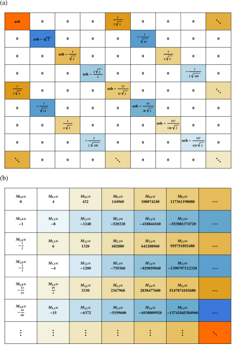
Figure 1: (a) The first $8\times 8$ matrix elements of the Born-Jordan parity operator from Eq. (49) where $\mathrm{ash}$ denotes $\mathrm{arcsinh}(1)$. (b) The first $6\times 6$ elements of the recursive sequence that defines the Born-Jordan parity operator via Eq. (54). Orange and blue colors represent positive and negative values, respectively, while the color intensity reflects the absolute value of the corresponding numbers.

Figure 1(a) shows the first $8\times 8$ entries of $[\mathrm{\Pi}_{\textup{BJ}}]$. One observes the following structure: only every fourth off-diagonal is non-zero, the matrix is real and symmetric, and the entries along every diagonal and off-diagonal decrease in their absolute value. In particular, the diagonal elements of $\mathrm{\Pi}_{\textup{BJ}}$ admit the following special property.

Proposition 3

For every $n\in\{0,1,2,\ldots\}$, the diagonal entries of $\mathrm{\Pi}_{\textup{BJ}}$ in the Fock basis are

$$[\mathrm{\Pi}_{\textup{BJ}}]_{nn}=\operatorname{arcsinh}(1)-\sqrt{2}\sum_{k=0}^{n-1}\frac{(-1)^{k}}{k{+}1}\sum_{m=0}^{\lfloor\frac{k}{2}\rfloor}\binom{2m}{m}\Big{(}\frac{-1}{4}\Big{)}^{m}.$$ (53)

In particular, $[\mathrm{\Pi}_{\textup{BJ}}]_{nn}\to 0$ as $n\to\infty$. For a proof we refer to Appendix I.

Also note that the sum of these decreasing diagonal entries results in a trace $\mathrm{Tr}[\mathrm{\Pi}_{\textup{BJ}}]=1/2$ (Property 6) in the number-state basis. However, this trace does not necessarily exist in an arbitrary basis, as $\mathrm{\Pi}_{\textup{BJ}}$ is not a trace-class operator.

Remark 11

Let us emphasize that the boundedness of $\mathrm{\Pi}_{\textup{BJ}}$ (Proposition 2) guarantees that using a (large enough) finite block of $\mathrm{\Pi}_{\textup{BJ}}$ for computations yields a good approximation. The reason for this is that such a block does not differ too much (in trace norm) from the full operator, which readily transfers to the phase-space distribution function. Details can be found at the end of Appendix C.

In the following, we specify a more convenient form for the calculation of these matrix elements, i.e. a direct recursion without summation, which is based on the following conjecture (see Appendix J).

Conjecture 1

The non-zero matrix elements

$$[\mathrm{\Pi}_{\textup{BJ}}]_{k+4\ell,k}=[\mathrm{\Pi}_{\textup{BJ}}]_{k,k+4\ell}=\Gamma_{k\ell}\,[M_{k\ell}+\delta_{\ell 0}\,\mathrm{arcsh}(1)/\sqrt{2}],$$ (54)

of the Born-Jordan parity operator are determined by a set of rational numbers $M_{k\ell}$ where $\Gamma_{k\ell}=2^{-2\ell+{1}/{2}}\sqrt{{k!}/{(k{+}4\ell)!}}$ and $k,\ell\in\{0,1,2,\dots\}$. The indexing is specified relative to the diagonal (where $\ell=0$) and $\delta_{\ell{}m}$ is the Kronecker delta. The rational numbers $M_{k\ell}$ can be calculated recursively using only 8 numbers as initial conditions, refer to Appendix J for details. This form does not require a summation.

Figure 1(b) shows the first $6\times 6$ elements of the recursive sequence of rational numbers $M_{k\ell}$. The first column of $M_{k0}$ corresponds to the diagonal of the matrix $[\mathrm{\Pi}_{\textup{BJ}}]_{mn}$ from Figure 1(a). For example, for $k=5$ one obtains $M_{5,0}=-{43}/{60}$, which corresponds to $[\mathrm{\Pi}_{\textup{BJ}}]_{5,5}=\Gamma_{5,0}[M_{5,0}+\delta_{0,0}\,\mathrm{arcsh}(1)/\sqrt{2}]$ and $\Gamma_{5,0}=\sqrt{2}$, and therefore $[\mathrm{\Pi}_{\textup{BJ}}]_{5,5}=-{43\sqrt{2}}/{60}+\mathrm{arcsh}(1)$ as detailed in Figure 1(a).

The direct recursion in Conjecture 1 enables us to conveniently and efficiently calculate the matrix elements $[\mathrm{\Pi}_{\textup{BJ}}]_{mn}$ and we have verified the correctness of this approach for up to $6400$ matrix elements, i.e. by calculating a matrix representation of size $80\times 80$. This facilitates an efficient calculation and plotting of Born-Jordan distributions for harmonic oscillator systems, such as in quantum optics mandel1995 ; glauber2007 ; leonhardt97 . Note that a recursively calculated $80\times 80$ matrix representation, which we have verified with exact calculations, is sufficient for most physical applications, i.e. Figures 2 and 3 (below) were calculated using $30\times 30$ matrix representations. However, a matrix representation of size $2000\times 2000$ can be easily calculated on a current notebook computer using the recursive method. Numerical evidence shows that the matrix representation of $\mathrm{\Pi}_{\textup{BJ}}$ can be well-approximated by a low-rank matrix, i.e, diagonalizing the matrix $\mathrm{\Pi}_{\textup{BJ}}$ reveals only very few significant eigenvalues. In particular, the sum of squares of the first $9$ eigenvalues corresponds to approximately $99.97\%$ of the sum of squares of all the eigenvalues of a $2000\times 2000$ matrix representation.

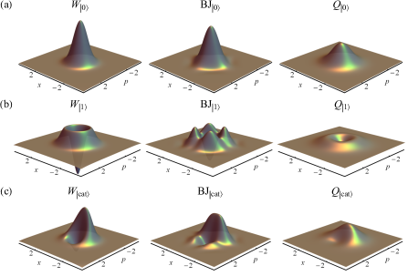
Figure 2: (a) and (b) Wigner, Born-Jordan, and Husimi Q phase-space plots of the number states $|0\rangle$ and $|1\rangle$ (which are eigenstates of the quantum harmonic oscillator). (c) Corresponding phase-space plots of the Schrödinger cat state $|\textup{cat}\rangle=(|0\rangle{+}|1\rangle)/\sqrt{2}$ (which is a superposition of the previous states).

7 Example Quantum States

Matrix representations of parity operators are used to conveniently calculate phase-space representations for bosonic quantum states via their associated Laguerre polynomial decompositions. The $s$-parametrized distribution functions of Fock states $|n\rangle$ are sums

$$F_{|n\rangle}(\mathrm{\Omega},s)=\sum_{\mu=0}|[\mathcal{D}(\mathrm{\Omega})]_{n\mu}|^{2}\,[\mathrm{\Pi}_{s}]_{\mu\mu}$$

of the associated Laguerre polynomials from (9), which are weighted by their parity operator elements. The corresponding phase-space functions are radially symmetric as $|[\mathcal{D}(\mathrm{\Omega})]_{n\mu}|^{2}$ depends only on the radial distance $x^{2}+p^{2}$. The Wigner functions in Fig. 2(a)-(b) are radially symmetric and show strong oscillations, which are sometimes regarded as a quantum-mechanical feature leonhardt97 .

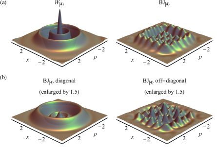
Figure 3: (a) Wigner and Born-Jordan phase-space plots of the number state $|4\rangle$. (b) The Born-Jordan distribution is decomposed into functions that correspond to diagonal and off-diagonal entries of the parity operator matrix.

In contrast, the Born-Jordan parity operator is not diagonal in the number state representation and it can be written in terms of projectors as $\mathrm{\Pi}_{\textup{BJ}}=\sum_{\mu=0}[\mathrm{\Pi}_{\textup{BJ}}]_{\mu\mu}|\mu\rangle\langle\mu|+\sum_{\mu=0}\sum_{\nu=1}[\mathrm{\Pi}_{\textup{BJ}}]_{\mu,4\nu}\,(|\mu{+}4\nu\rangle\langle\mu|+|\mu\rangle\langle\mu{+}4\nu|),$ and the Born-Jordan distribution of number states $|n\rangle$ is given by

$$F_{|n\rangle}(\mathrm{\Omega},\textup{BJ}) =\sum_{\mu=0}|[\mathcal{D}]_{n\mu}|^{2}\,[\mathrm{\Pi}_{\textup{BJ}}]_{\mu\mu}$$ (55)

$$+\sum_{\mu=0}\sum_{\nu=1}2\,\Re([\mathcal{D}]_{n\mu}([\mathcal{D}]_{n,\mu+4\nu})^{*})[\mathrm{\Pi}_{\textup{BJ}}]_{\mu,\mu+4\nu}.$$ (56)

The Born-Jordan distribution of coherent states, i.e. the displaced vacuum states, closely matches the Wigner functions, see Fig. 2(a). The first part in Eq. (55) contains the diagonal elements of the parity operator which correspond to the radially symmetric part of $F_{|n\rangle}(\mathrm{\Omega},\textup{BJ})$, see Fig. 3(b) (left). The second part in Eq. (56) results in a radially non-symmetric function, see Fig. 3(b) (right). The radially symmetric parts are quite similar to the Wigner function and have $n+1$ wave fronts enclosed by the Bohr-Sommerfeld band leonhardt97 ; dowling1991 , i.e. the ring with radius $\sqrt{2n{+}1}$. The radially non-symmetric functions have $n+1$ local maxima along the outer squares, i.e. along phase-space cuts at the Bohr-Sommerfeld distance $x,p\propto\sqrt{2n{+}1}$. The sum of these two contributions is the Born-Jordan distribution and it is not radially symmetric for number states, see Fig. 3(a).

8 Conclusion

We have introduced parity operators $\mathrm{\Pi}_{\theta}$ which give rise to a rich family of phase-space distribution functions of quantum states. These phase-space functions have been previously defined in terms of convolutions, integral transformations, or Fourier transformations. Our approach using parity operators is both conceptually and computationally advantageous and now allows for a direct calculation of phase-space functions as quantum-mechanical expectation values. This approach therefore averts the necessity for the repeated and expensive computation of Fourier transformations. We motivate the name “parity operator” by the fact that parity operators $\mathrm{\Pi}_{\theta}=A_{\theta}\circ\mathrm{\Pi}$ are composed of the usual parity operator and some specific geometric or physical transformation. We detailed the explicit form of parity operators for various phase spaces and, in particular, for the Born-Jordan distribution. We have also obtained a generalized spectral decomposition of the Born-Jordan parity operator, proved its boundedness, and explicitly calculated its matrix representation in the number-state basis. We conjecture that these matrix elements are determined by a proposed recursive scheme which allows for an efficient computation of Born-Jordan distribution functions. Moreover, large matrix representations of the Born-Jordan parity operator can be well approximated using rank-9 matrices. All this will be useful to connect our results with applications in (e.g.) quantum optics, where techniques such as squeezing operators and the number-state representation are widely used.

Appendix A Extension of Operators from Schwartz Functions to Distributions

Assume we have a linear operator $T:\mathcal{S}(\mathbb{R})\to\mathcal{S}(\mathbb{R})$ or, more generally, $T:\mathcal{S}(\mathbb{R})\to(\mathbb{R}\to\mathbb{C})$ and we want to extend its action to tempered distributions. Usually this is done by introducing some operator $\hat{T}:\mathcal{S}(\mathbb{R})\to(\mathbb{R}\to\mathbb{C})$ (which can—but does not have to—be the same as $T$) such that

$$(T\phi)(\psi):=\phi(\hat{T}\psi)$$ (57)

for all $\phi\in D_{T}:=\{\phi\in\mathcal{S}^{\prime}(\mathbb{R}):\phi\circ\hat{T}\in\mathcal{S}^{\prime}(\mathbb{R})\}$ and all $\psi\in\mathcal{S}(\mathbb{R})$. Usually $\hat{T}$ is chosen such that (57) is consistent with the action of $T$ on those distributions which are generated by Schwartz functions. More precisely one fixes some injective, usually linear or antilinear map $e:\mathcal{S}(\mathbb{R})\to\mathcal{S}^{\prime}(\mathbb{R})$ and requires that $\hat{T}$ is chosen such that $[T,e]\equiv 0$, i.e.

$$e(\phi)(\hat{T}\psi)=\big{(}T(e(\phi))\big{)}(\psi)=\big{(}(T\circ e)(\phi)\big{)}(\psi)=\big{(}(e\circ T)(\phi)\big{)}(\psi)=e(T\phi)(\psi)$$

for all $\phi,\psi\in\mathcal{S}(\mathbb{R})$ with $e(\phi)\in D_{T}$. Thus by identifying functions $\phi\in\mathcal{S}(\mathbb{R})$ with the tempered distribution $e(\phi)\in\mathcal{S}^{\prime}(\mathbb{R})$ an extension is defined such that there is only a “formal” difference between the action of $T$ on $\phi$ compared to the action of $T$ on $e(\phi)$. Let us illustrate this by means of a simple example:

Example 3

Consider the displacement operator from Eq. (10) which acts on any function $\psi:\mathbb{R}\to\mathbb{C}$—so in particular on any Schwartz function—via $[\mathcal{D}(x_{0},p_{0})\psi](x)=\exp[{{i}p_{0}(x{-}x_{0}/2)/\hbar}]\psi(x{-}x_{0})$ for all $x,x_{0},p_{0}\in\mathbb{R}$. Depending on how one defines the distributional pairing of two classical functions there are two ways to extend $\mathcal{D}$ to $\mathcal{S}^{\prime}(\mathbb{R})$:

(1) The usual way of embedding $\mathcal{S}(\mathbb{R})\hookrightarrow\mathcal{S}^{\prime}(\mathbb{R})$ is done via the linear map $\iota(\psi):=\int\psi(x)(\cdot)(x)\,\mathrm{d}x$. Then for all $\phi,\psi\in\mathcal{S}(\mathbb{R})$ and all $\mathrm{\Omega}\in\mathbb{R}^{2}$ one finds (thewignertransform, , Eq. (1.11))

$$\iota(\phi)\big{(}\mathcal{D}(\Omega)\psi\big{)}=\iota\big{(}\mathcal{D}^{\wedge x}(\mathrm{\Omega})\phi\big{)}\psi\qquad\text{ or, equivalently }\qquad\iota\big{(}\mathcal{D}(\mathrm{\Omega})\phi\big{)}\psi=\iota(\phi)\big{(}\mathcal{D}^{\wedge x}(\Omega)\psi\big{)}$$

where $\mathcal{D}^{\wedge x}(x_{0},p_{0}):=\mathcal{D}(-x_{0},p_{0})$ for all $x_{0},p_{0}\in\mathbb{R}$. This suggests setting $\hat{T}:=\mathcal{D}^{\wedge x}$ in (57) because this way one has $[\mathcal{D}(\mathrm{\Omega}),\iota]\equiv 0$, that is, $\mathcal{D}(\mathrm{\Omega})(\iota(\phi))\equiv\iota(\mathcal{D}(\mathrm{\Omega})\phi)$ for all $\mathrm{\Omega}\in\mathbb{R}^{2}$ and all $\phi:\mathbb{R}\to\mathbb{C}$ such that $\int\phi(x)(\cdot)(x)\,\mathrm{d}x\in\mathcal{S}^{\prime}(\mathbb{R})$. In other words this extension of the displacement operator is consistent with its action on $\mathcal{S}(\mathbb{R})$ by means of the embedding $\iota$.

(2) One may also consider the canonical (antilinear, bijective) map from $L^{2}(\mathbb{R})$ to its dual space $(L^{2}(\mathbb{R}))^{*}$ from the Riesz representation theorem which acts via $\langle\,\cdot\,|\;(\psi):=\langle\psi|\,\cdot\,\rangle:=\int\psi(x)^{*}(\cdot)(x)\,\mathrm{d}x$. One readily verifies that $\langle\phi|\mathcal{D}(\mathrm{\Omega})\psi\rangle=\langle\mathcal{D}(-\mathrm{\Omega})\phi|\psi\rangle$ for all $\phi,\psi\in L^{2}(\mathbb{R})$, i.e. $D(\mathrm{\Omega})^{\dagger}=\mathcal{D}(-\mathrm{\Omega})$ for all $\mathrm{\Omega}\in\mathbb{R}^{2}$. Setting $\hat{T}:=\mathcal{D}(\mathrm{\Omega})^{\dagger}$ in (57) thus yields an extension of $\mathcal{D}$ which is consistent with respect to $\langle\,\cdot\,|\;$: one finds $[\mathcal{D}(\mathrm{\Omega})\langle\,\cdot\,|\;]\equiv 0$, that is, for all $\phi,\psi\in\mathcal{S}(\mathbb{R})$

$$\mathcal{D}(\mathrm{\Omega})(\langle\phi,\cdot\,\rangle)(\psi)\overset{\eqref{eq:extension_def}}{=}\langle\phi,\mathcal{D}(-\mathrm{\Omega})\psi\rangle=\langle\mathcal{D}(\mathrm{\Omega})\phi,\psi\rangle=\langle\mathcal{D}(\mathrm{\Omega})\phi,\cdot\,\rangle(\psi).$$

Having introduced the concept of operator extensions we may apply it to generalized parity operators. But first let us generalize Definition 3 to arbitrary tempered distributions $\theta$, even though this is beyond what we need in the main sections of this article.

Remark 12

Formally (21) can be rewritten as $\Pi_{\theta}=(4\pi\hbar)^{-1}\langle K_{\theta}^{*},\mathcal{D}\rangle$. Because admissible kernels by definition satisfy $\langle K_{\theta}^{*},\psi\rangle=2\pi\hbar[\mathcal{F}_{\sigma}(\theta)]\psi$ for $\psi\in\mathcal{S}(\mathbb{R})$ this leads to an extension of Definition 3 to arbitrary $\theta\in\mathcal{S}^{\prime}(\mathbb{R}^{2})$ via the linear operator $\Pi_{\theta}:\mathcal{S}(\mathbb{R})\to(\mathbb{R}\to\mathbb{C})$, $\Pi_{\theta}:=\frac{1}{2}[\mathcal{F}_{\sigma}(\theta)\circ\mathcal{D}]$, i.e.

$$(\Pi_{\theta}\psi)(x)=\tfrac{1}{2}\mathcal{F}_{\sigma}(\theta)(\mathcal{D}\psi(x))=\tfrac{1}{2}\theta\big{(}\mathcal{F}_{\sigma}(\mathcal{D}\psi(x))\big{)}$$

for all $\psi\in\mathcal{S}(\mathbb{R})$, $x\in\mathbb{R}$. Here $\mathcal{D}\psi(x)\in\mathcal{S}(\mathbb{R}^{2})$ defined via $\Omega\mapsto(\mathcal{D}(\Omega)\psi)(x)$ is the displacement of $\psi$ at $x$ as a function of $\Omega$. One readily verifies that for admissible kernels this definition reproduces (24) as well as the definition of the parity operator in (14).

Similar to Example 3(1), let us extend $\Pi_{\theta}$ with respect to the embedding $\iota:\mathcal{S}(\mathbb{R})\hookrightarrow\mathcal{S}^{\prime}(\mathbb{R})$, that is, we have to find an operator $\tilde{\Pi}_{\theta}:\mathcal{S}(\mathbb{R})\to(\mathbb{R}\to\mathbb{C})$ such that $\iota(\phi)(\tilde{\Pi}_{\theta}\psi)=\iota(\Pi_{\theta}\phi)(\psi)$ for all $\psi,\phi\in\mathcal{S}(\mathbb{R})$. We claim that

$$\tilde{\Pi}_{\theta}:=\tfrac{1}{2}[\mathcal{F}_{\sigma}(\theta^{\wedge p})\circ\mathcal{D}]$$ (58)

does the job where $\theta^{\wedge p}(a):=\theta(a^{\wedge p})$ and $a^{\wedge p}(x_{0},p_{0}):=a(x_{0},-p_{0})$ for all $a\in\mathcal{S}(\mathbb{R}^{2})$, $x_{0},p_{0}\in\mathbb{R}$. Before we verify this we will first show $\iota(\phi)\big{(}\mathcal{F}_{\sigma}[\mathcal{D}\psi](x_{0},-p_{0})\big{)}=\iota\big{(}\mathcal{F}_{\sigma}[\mathcal{D}\phi](x_{0},p_{0})\big{)}(\psi)$ for all $\phi,\psi\in\mathcal{S}(\mathbb{R})$, $x_{0},p_{0}\in\mathbb{R}$ as an intermediate result. One computes

$$\iota(\phi)\big{(}\mathcal{F}_{\sigma}[\mathcal{D}\psi](x_{0},-p_{0})\big{)}=(2\pi\hbar)^{-1}\int\phi(x)\int e^{-\frac{i}{\hbar}(x^{\prime}(-p_{0})-x_{0}p^{\prime})}\big{(}\mathcal{D}(x^{\prime},p^{\prime})\psi\big{)}(x)\,\mathrm{d}x^{\prime}\,\mathrm{d}p^{\prime}\,\mathrm{d}x$$

$$=(2\pi\hbar)^{-1}\int\phi(x)\int e^{-\frac{i}{\hbar}(x^{\prime}(-p_{0})-x_{0}p^{\prime})}e^{\frac{i}{\hbar}p^{\prime}(x-\frac{1}{2}x^{\prime})}\psi(x{-}x^{\prime})\,\mathrm{d}x^{\prime}\,\mathrm{d}p^{\prime}\,\mathrm{d}x$$

$$=(2\pi\hbar)^{-1}\int\phi(x{+}x^{\prime})\int e^{-\frac{i}{\hbar}((-x^{\prime})p_{0}-x_{0}p^{\prime})}e^{\frac{i}{\hbar}p^{\prime}(x+\frac{1}{2}x^{\prime})}\psi(x)\,\mathrm{d}x^{\prime}\,\mathrm{d}p^{\prime}\,\mathrm{d}x$$

$$=\int\Big{(}(2\pi\hbar)^{-1}\int e^{-\frac{i}{\hbar}(\tilde{x}p_{0}-x_{0}p^{\prime})}e^{\frac{i}{\hbar}p^{\prime}(x-\frac{1}{2}\tilde{x})}\phi(x{-}\tilde{x})\,\mathrm{d}\tilde{x}\,\mathrm{d}p^{\prime}\Big{)}\psi(x)\,\mathrm{d}x$$

$$=\int\mathcal{F}_{\sigma}[\mathcal{D}\phi(x)](x_{0},p_{0})\psi(x)\,\mathrm{d}x=\iota\big{(}\mathcal{F}_{\sigma}[\mathcal{D}\phi](x_{0},p_{0})\big{)}(\psi).$$

Together with the linearity of the integral as well as the linearity and continuity of $\theta$ this implies

$$\iota(\phi)(\tfrac{1}{2}[\mathcal{F}_{\sigma}(\theta^{\wedge p})\circ\mathcal{D}]\psi)=\tfrac{1}{2}\int\phi(x)\theta\big{(}\big{(}\mathcal{F}_{\sigma}(\mathcal{D}\psi(x))\big{)}^{\wedge p}\big{)}\,\mathrm{d}x$$

$$=\tfrac{1}{2}\theta\Big{(}\int\phi(x)\big{(}\mathcal{F}_{\sigma}(\mathcal{D}\psi(x))\big{)}^{\wedge p}\,\mathrm{d}x\Big{)}=\tfrac{1}{2}\theta\Big{(}\int\mathcal{F}_{\sigma}(\mathcal{D}\phi(x))\psi(x)\,\mathrm{d}x\Big{)}$$

$$=\tfrac{1}{2}\int\theta\big{(}\mathcal{F}_{\sigma}(\mathcal{D}\phi(x))\big{)}\psi(x)\,\mathrm{d}x=\iota\big{(}\tfrac{1}{2}[\mathcal{F}_{\sigma}(\theta)\circ\mathcal{D}]\phi\big{)}(\psi)$$

for all $\phi,\psi\in\mathcal{S}(\mathbb{R})$. Thus by setting $T=\Pi_{\theta}$ and $\hat{T}=\tilde{\Pi}_{\theta}$ in (57) with $\tilde{\Pi}_{\theta}$ from (58), that is,

$$(\Pi_{\theta}\phi)(\psi):=\tfrac{1}{2}\phi\big{[}\theta\big{(}\big{(}\mathcal{F}_{\sigma}[\mathcal{D}\psi]\big{)}^{\wedge p}\big{)}\big{]}$$

for all $\psi\in\mathcal{S}(\mathbb{R})$, $\phi\in D_{\theta}:=\{\phi\in\mathcal{S}^{\prime}(\mathbb{R}):\phi\big{[}\theta\big{(}\big{(}\mathcal{F}_{\sigma}(\mathcal{D}(\cdot))\big{)}^{\wedge p}\big{)}\big{]}\in\mathcal{S}^{\prime}(\mathbb{R})\}$ we get an extension of $\Pi_{\theta}$ which is compatible with the integral pairing $\iota$ in the sense that $[\Pi_{\theta},\iota]\equiv 0$.

Now as in Example 3(2), let us extend $\Pi_{\theta}$ with respect to $\langle\,\cdot\,|:L^{2}(\mathbb{R})\to(L^{2}(\mathbb{R}))^{*}$. We claim that

$$\tilde{\Pi}_{\theta}:=\tfrac{1}{2}[\mathcal{F}_{\sigma}(\;{}^{*}\circ\theta\circ{}^{*}\;)\circ\mathcal{D}]$$ (59)

satisfies $\langle\phi,\tilde{\Pi}_{\theta}\psi\rangle=\langle\Pi_{\theta}\phi,\psi\rangle$ for all $\psi,\phi\in\mathcal{S}(\mathbb{R})$, where ^∗ is the usual complex conjugate. Similar as before, one first shows

$$\int\big{(}\mathcal{F}_{\sigma}[\mathcal{D}\psi(x)](x_{0},p_{0})\big{)}^{*}\phi(x)\,\mathrm{d}x=\int\psi(x)^{*}\mathcal{F}_{\sigma}[\mathcal{D}\phi(x)](x_{0},p_{0})\,\mathrm{d}x$$

via direct calculation in order to conclude that

$$\langle\phi,\tilde{\Pi}_{\theta}\psi\rangle =\tfrac{1}{2}\int\phi(x)^{*}\big{(}\theta\big{[}(\mathcal{F}_{\sigma}(\mathcal{D}\psi(x)))^{*}\big{]}\big{)}^{*}\,\mathrm{d}x=\tfrac{1}{2}\Big{(}\int\phi(x)\theta\big{[}(\mathcal{F}_{\sigma}(\mathcal{D}\psi(x)))^{*}\big{]}\,\mathrm{d}x\Big{)}^{*}$$

$$=\tfrac{1}{2}\Big{(}\theta\Big{[}\int\big{(}\mathcal{F}_{\sigma}(\mathcal{D}\psi(x))\big{)}^{*}\phi(x)\,\mathrm{d}x\Big{]}\Big{)}^{*}=\tfrac{1}{2}\Big{(}\theta\Big{[}\int\psi(x)^{*}\mathcal{F}_{\sigma}(\mathcal{D}\phi(x))\,\mathrm{d}x\Big{]}\Big{)}^{*}$$

$$=\tfrac{1}{2}\int\big{(}\theta\big{[}\mathcal{F}_{\sigma}(\mathcal{D}\phi(x))\big{]}\big{)}^{*}\psi(x)\,\mathrm{d}x=\langle\Pi_{\theta}\phi,\psi\rangle$$

for all $\phi,\psi\in\mathcal{S}(\mathbb{R})$. Hence $\tilde{\Pi}_{\theta}=\tfrac{1}{2}[\mathcal{F}_{\sigma}(\;{}^{*}\circ\theta\circ{}^{*}\;)\circ\mathcal{D}]$ is indeed the extension of $\Pi_{\theta}$ with respect to $\langle\,\cdot\,|$ which we were looking for.

In general these two extensions will be different so one has to be careful about which framework one uses. However from the explicit form of $\tilde{\Pi}_{\theta}$ one knows that for any $\theta\in\mathcal{S}^{\prime}(\mathbb{R}^{2})$ these extensions coincide if and only if $\theta^{\wedge p}\equiv{}^{*}\circ\theta\circ{}^{*}\,$. This translates to filter functions as follows:

Lemma 3

Consider any admissible $\theta\in\mathcal{S}^{\prime}(\mathbb{R}^{2})$ with associated filter function $K_{\theta}:\mathbb{R}^{2}\to\mathbb{C}$. The extension of $\Pi_{\theta}$ with respect to $\iota$ coincides with the extension of $\Pi_{\theta}$ with respect to $\langle\,\cdot\,|\;$ if and only if $K_{\theta}^{*}\equiv K_{\theta}^{\wedge p}$. In this case (57) becomes

$$(\Pi_{\theta}\phi)(\psi) =(4\pi\hbar)^{-1}\int K_{\theta}^{*}(\Omega)\phi\big{(}\mathcal{D}(-\Omega)\psi\big{)}\,\mathrm{d}\mathrm{\Omega}$$

$$=(4\pi\hbar)^{-1}\int K_{\theta}(x_{0},p_{0})\phi\big{(}\mathcal{D}(-x_{0},p_{0})\psi\big{)}\,\mathrm{d}x_{0}\mathrm{d}p_{0}$$

for all $\phi\in\mathcal{S}^{\prime}(\mathbb{R})$ such that $\int K_{\theta}^{*}(\Omega)\phi\big{[}\mathcal{D}(-\Omega)(\cdot)\big{]}\,\mathrm{d}\mathrm{\Omega}\in\mathcal{S}^{\prime}(\mathbb{R})$, and all $\psi\in\mathcal{S}(\mathbb{R})$.

Proof

Because $\theta$ is admissible (i.e. $\theta=(2\pi\hbar)^{-1}\langle K_{\theta}^{*},\mathcal{F}_{\sigma}(\cdot)\,\rangle$ for some $K_{\theta}:\mathbb{R}^{2}\to\mathbb{C}$) we compute

$$\mathcal{F}_{\sigma}({}^{*}\circ\theta\circ{}^{*})(a)=\big{(}\theta\big{[}\mathcal{F}_{\sigma}(a)^{*}\big{]}\big{)}^{*}=(2\pi\hbar)^{-1}\Big{(}\int K_{\theta}(\mathrm{\Omega})\mathcal{F}_{\sigma}\big{[}\mathcal{F}_{\sigma}(a)^{*}\big{]}(\mathrm{\Omega})\,\mathrm{d}\mathrm{\Omega}\Big{)}^{*}$$

$$=(2\pi\hbar)^{-1}\Big{(}\int K_{\theta}(\mathrm{\Omega})\mathcal{F}_{\sigma}\big{[}\mathcal{F}_{\sigma}(a)\big{]}^{*}(-\mathrm{\Omega})\,\mathrm{d}\mathrm{\Omega}\Big{)}^{*}=(2\pi\hbar)^{-1}\int K_{\theta}^{*}(\mathrm{\Omega})a(-\mathrm{\Omega})\,\mathrm{d}\mathrm{\Omega}$$

for all $a\in\mathcal{S}(\mathbb{R}^{2})$. Here we used $\mathcal{F}_{\sigma}^{2}=\operatorname{id}$ as well as the readily verified identity $\mathcal{F}_{\sigma}[a^{*}](\Omega)=\mathcal{F}_{\sigma}[a]^{*}(-\Omega)$. If we denote the extension of $\Pi_{\theta}$ with respect to $\langle\,\cdot\,|$ by $\Pi_{\theta,L^{2}}$ this implies

$$(\Pi_{\theta,L^{2}}\phi)(\psi)=\tfrac{1}{2}\phi\big{(}\mathcal{F}_{\sigma}(\;{}^{*}\circ\theta\circ{}^{*}\;)[\mathcal{D}\psi]\big{)}=(4\pi\hbar)^{-1}\int K_{\theta}^{*}(\mathrm{\Omega})\phi\big{(}\mathcal{D}(-\mathrm{\Omega})\psi\big{)}\,\mathrm{d}\mathrm{\Omega}.$$

On the other hand the symplectic nature of $\mathcal{F}_{\sigma}$ yields $\mathcal{F}_{\sigma}(a^{\wedge p})=(\mathcal{F}_{\sigma}(a))^{\wedge x}$ for all $a\in\mathcal{S}(\mathbb{R}^{2})$ (where $a^{\wedge x}(x_{0},p_{0}):=a(-x_{0},p_{0})$). Similarly let $\Pi_{\theta,\iota}$ denote the extension of $\Pi_{\theta}$ with respect to $\iota$; this lets us compute

$$(\Pi_{\theta,\iota}\phi)(\psi)=(4\pi\hbar)^{-1}\int K_{\theta}(\mathrm{\Omega})\phi\Big{(}\mathcal{F}_{\sigma}\big{[}\big{(}\mathcal{F}_{\sigma}[\mathcal{D}\psi]\big{)}^{\wedge p}\big{]}(\mathrm{\Omega})\Big{)}\,\mathrm{d}\mathrm{\Omega}$$

$$=(4\pi\hbar)^{-1}\int K_{\theta}(\mathrm{\Omega})\phi\Big{(}\mathcal{F}_{\sigma}\big{[}\big{(}\mathcal{F}_{\sigma}[\mathcal{D}\psi]\big{)}\big{]}^{\wedge x}(\mathrm{\Omega})\Big{)}\,\mathrm{d}\mathrm{\Omega}$$

$$=(4\pi\hbar)^{-1}\int K_{\theta}(x_{0},p_{0})\phi\big{(}\mathcal{D}(-x_{0},p_{0})\psi\big{)}\,\mathrm{d}x_{0}\mathrm{d}p_{0}$$

$$=(4\pi\hbar)^{-1}\int K_{\theta}(x_{0},-p_{0})\phi\big{(}\mathcal{D}(-x_{0},-p_{0})\psi\big{)}\,\mathrm{d}x_{0}\mathrm{d}p_{0}.$$

Thus $\Pi_{\theta,\iota}\equiv\Pi_{\theta,L^{2}}$ is equivalent to $K_{\theta}^{*}\equiv K_{\theta}^{\wedge p}$ as claimed.∎

We emphasize that all filter functions used in practice satisfy $K_{\theta}^{*}\equiv K_{\theta}^{\wedge p}$ (cf. Tables 2 and 3), so it does not matter for applications whether one extends $\Pi_{\theta}$ with respect to $\iota$ or $\langle\,\cdot\,|$.

Appendix B Proofs of Lemma 2 and Theorem 4.1

Before we dive into the proofs of the results in question we first need a lemma which relates convolutions of the cross-Wigner transform with matrix elements of the generalized Grossmann-Royer operator.

Lemma 4

Given any $\theta\in\mathcal{S}^{\prime}(\mathbb{R}^{2})$ one finds

$$\langle\phi,\mathcal{D}(\mathrm{\Omega})\Pi_{\theta}\mathcal{D}^{\dagger}(\mathrm{\Omega})\psi\rangle=\pi\hbar[\theta\ast W_{\phi,\psi}](\mathrm{\Omega})$$ (60)

for all $\phi,\psi\in\mathcal{S}(\mathbb{R})$ and all $\mathrm{\Omega}\in\mathbb{R}^{2}$. If $\Pi_{\theta}\in\mathcal{B}(L^{2}(\mathbb{R}))$ then Eq. (60) even holds for all $\phi,\psi\in L^{2}(\mathbb{R})$.

Proof

Sums in the argument of the displacement operator decompose as (see Eq. (13) and (thewignertransform, , Eq. (1.10))):

$$\mathcal{D}(\mathrm{\Omega}{-}\mathrm{\Omega}^{\prime})=e^{-\frac{i}{2\hbar}(xp^{\prime}-x^{\prime}p)}\mathcal{D}(\mathrm{\Omega})\mathcal{D}(-\mathrm{\Omega}^{\prime}).$$

This lets us connect the r.h.s. of (60) with the Grossmann-Royer operator (15):

$$\langle\phi,[\mathcal{T}(\mathrm{\Omega})\mathcal{D}]^{\dagger}(\mathrm{\Omega}^{\prime})\Pi[\mathcal{T}(\mathrm{\Omega})\mathcal{D}](\mathrm{\Omega}^{\prime})\psi\rangle=\langle\phi,\mathcal{D}(\mathrm{\Omega}{-}\mathrm{\Omega}^{\prime})\Pi\mathcal{D}^{\dagger}(\mathrm{\Omega}{-}\mathrm{\Omega}^{\prime})\psi\rangle$$

$$=\langle\phi,\mathcal{D}(\mathrm{\Omega})\mathcal{D}(-\mathrm{\Omega}^{\prime})\Pi\mathcal{D}^{\dagger}(-\mathrm{\Omega}^{\prime})\mathcal{D}^{\dagger}(\mathrm{\Omega})\psi\rangle=\langle\mathcal{D}(-\mathrm{\Omega})\phi,\tfrac{1}{2}\mathcal{F}_{\sigma}[\mathcal{D}(\cdot)\mathcal{D}(-\mathrm{\Omega})\psi](\mathrm{\Omega}^{\prime})\rangle$$

Together with linearity and continuity of $\theta$ this implies

$$\pi\hbar[\theta\ast W_{\phi,\psi}](\mathrm{\Omega})=\theta\big{(}\langle\phi,[\mathcal{T}(\mathrm{\Omega})\mathcal{D}]^{\dagger}(\cdot)\Pi[\mathcal{T}(\mathrm{\Omega})\mathcal{D}](\cdot)\psi\rangle\big{)}$$

$$=\theta\big{(}\langle\mathcal{D}(-\mathrm{\Omega})\phi,\tfrac{1}{2}\mathcal{F}_{\sigma}[\mathcal{D}(\cdot)\mathcal{D}(-\mathrm{\Omega})\psi]\rangle\big{)}=\langle\phi,\mathcal{D}(\mathrm{\Omega})\tfrac{1}{2}\theta\big{[}\mathcal{F}_{\sigma}\big{(}(\mathcal{D}(\cdot)\mathcal{D}(-\mathrm{\Omega})\psi)\big{)}\big{]}\rangle$$

$$=\langle\phi,\mathcal{D}(\mathrm{\Omega})\Pi_{\theta}\mathcal{D}(-\mathrm{\Omega})\psi\rangle=\langle\phi,\mathcal{D}(\mathrm{\Omega})\Pi_{\theta}\mathcal{D}^{\dagger}(\mathrm{\Omega})\psi\rangle.$$

In the second-to-last step we used the general definition of $\Pi_{\theta}$ from Remark 12. Now if $\Pi_{\theta}$ is bounded then the l.h.s. of (60) extends to all square-integrable functions by density of $\mathcal{S}(\mathbb{R})$ in $L^{2}(\mathbb{R})$.∎

Thus we have the (formal) equality $\langle\phi,\Pi_{\theta}\psi\rangle=\pi\hbar[\theta\ast W_{\phi,\psi}](0,0)$ for all $\phi,\psi:\mathbb{R}\to\mathbb{C}$ where this expression is well-defined. Using this we are ready to prove Lemma 2, in particular the equivalence of (i,a), (i,b) and (ii,a), (ii,b), (ii,c) for general $\theta\in\mathcal{S}^{\prime}(\mathbb{R}^{2})$.

B.1 Proof of Lemma 2

Proof (Lemma 2)

“(i,a) $\Rightarrow$ (i,b)”: Because $\Pi_{\theta}$ is well defined, $\psi\mapsto[\theta\ast W_{\psi}](0,0)=(\pi\hbar)^{-1}\langle\psi|\Pi_{\theta}\psi\rangle$ is well defined on $L^{2}(\mathbb{R})$ as well. “(i,b) $\Rightarrow$ (i,a)”: Assume that $\psi\mapsto[\theta\ast W_{\psi}](0,0)$ is well defined on $L^{2}(\mathbb{R})$. Then $\langle\psi|\Pi_{\theta}\psi\rangle=\pi\hbar[\theta\ast W_{\psi,\psi}](0,0)=\pi\hbar[\theta\ast W_{\psi}](0,0)$ exists for all $\psi\in L^{2}(\mathbb{R})$ and the same is true for $\langle\psi|\Pi_{\theta}\phi\rangle$ using the parallelogram law $4\langle\psi|\Pi_{\theta}\phi\rangle=\langle\psi{+}\phi|\Pi_{\theta}(\psi{+}\phi)\rangle-\langle\psi{-}\phi|\Pi_{\theta}(\psi{-}\phi)\rangle+i\langle\psi{-}i\phi|\Pi_{\theta}(\psi{-}i\phi)\rangle-i\langle\psi{+}i\phi|\Pi_{\theta}(\psi{+}i\phi)\rangle$. Hence $\tilde{\phi}\mapsto\int\tilde{\phi}(x)(\Pi_{\theta}\phi)(x)\,\mathrm{d}x$ is a well-defined linear functional on $L^{2}(\mathbb{R})$ meaning—because it is a functional “of integral pairing form”—it is automatically continuous as we prove now: If $\langle f,\cdot\,\rangle:L^{2}(\mathbb{R})\to\mathbb{C}$, $g\mapsto\int f(x)g(x)\,\mathrm{d}x$ is well defined for some $f:\mathbb{R}\to\mathbb{C}$, then $(\Re(fg))_{\pm}$, $(\Im(fg))_{\pm}$ are integrable by definition of the Lebesgue integral, where $f_{+}(x):=\max(f(x),0)$ and $f_{-}:=-\min(f(x),0)$. But these can be expanded into $(\Re(f))_{\pm}(\Re(g))_{\pm}$, $(\Re(f))_{\pm}(\Im(g))_{\pm}$, $(\Im(f))_{\pm}(\Re(g))_{\pm}$, $(\Im(f))_{\pm}(\Im(g))_{\pm}$ meaning the linear functionals $g\mapsto\int(\Re(f))_{\pm}g$ and $g\mapsto\int(\Im(f))_{\pm}g$ are also well defined on $L^{2}(\mathbb{R})$. Now each of these is a positive functional on $L^{2}(\mathbb{R})$ which is well known to be continuous (one can prove this similar to (Davies76, , Ch. 2, Lemma 2.1)). Therefore $\langle f,\cdot\,\rangle$ is continuous as it is the linear combination of four continuous functionals.

Then the Riesz representation theorem (cf., e.g., (ReedSimon1, , Supplementary Material, Thm. S.4)) yields $f\in L^{2}(\mathbb{R})$ such that $f^{*}(x)=(\Pi_{\theta}\phi)(x)$ for almost all $x\in\mathbb{R}$; in particular $\Pi_{\theta}\phi\in L^{2}(\mathbb{R})$. But $\phi\in L^{2}(\mathbb{R})$ was chosen arbitrarily meaning $\Pi_{\theta}$ is a well-defined linear operator on $L^{2}(\mathbb{R})$. The equivalence “(ii,a) $\Leftrightarrow$ (ii,b)” is obvious and “(ii,a) $\Leftrightarrow$ (ii,c)” follows at once from (60) together with

$$\sup_{\|\psi\|,\|\phi\|=1}|[\theta\ast W_{\phi,\psi}](0,0)|=\sup_{\|\psi\|,\|\phi\|=1}|\langle\phi|\Pi_{\theta}\psi\rangle|=\sup_{\|\phi\|=1}\|\Pi_{\theta}\phi\|_{L^{2}}=\|\Pi_{\theta}\|_{\mathrm{sup}}.$$

Now assume that $\theta$ is admissible. Because “(ii,c) $\Rightarrow$ (i,a)” is trivial, all that remains to show is “(i,a) $\Rightarrow$ (ii,c)”: Our idea is to show that $\theta$ being admissible implies that $\Pi_{\theta}$ can be written as the linear combination of two well-defined symmetric operators on $L^{2}(\mathbb{R})$. This would conclude the proof because every symmetric operator is bounded by the Hellinger-Toeplitz theorem (ReedSimon1, , p. 84), hence $\Pi_{\theta}$ is bounded as well. Set $K_{\theta^{*}}(\Omega):=K_{\theta}^{*}(-\Omega)$ and define $\Pi_{\theta^{*}}$ to be the parity operator generated by $K_{\theta^{*}}$. First we have to see whether $\Pi_{\theta}$ being well defined on $L^{2}(\mathbb{R})$ implies that the same holds for $\Pi_{\theta^{*}}$. Given $\psi,\phi\in L^{2}(\mathbb{R})$ we formally compute

$$\langle\psi|\mathrm{\Pi}_{\theta^{*}}\phi\rangle =(4\pi\hbar)^{-1}\int K_{\theta}^{*}(-\Omega)\langle\psi|\mathcal{D}(\Omega)\phi\rangle\,\mathrm{d}\Omega=(4\pi\hbar)^{-1}\int K_{\theta}^{*}(\tilde{\Omega})\langle\psi|\mathcal{D}^{\dagger}(\tilde{\Omega})\phi\rangle\,d\tilde{\Omega}$$

$$=(4\pi\hbar)^{-1}\int K_{\theta}^{*}(\tilde{\Omega})\big{(}\langle\phi|\mathcal{D}(\tilde{\Omega})\psi\rangle\big{)}^{*}\,d\tilde{\Omega}=(\langle\phi|\Pi_{\theta}\psi\rangle)^{*}.$$

Thus $\langle\psi|\mathrm{\Pi}_{\theta^{*}}\phi\rangle$ exists for all $\psi,\phi\in L^{2}(\mathbb{R})$ so by the same argument we used above, $\Pi_{\theta^{*}}$ is well defined on $L^{2}(\mathbb{R})$. This yields the decomposition $\Pi_{\theta}=(\Pi_{\theta}{+}\Pi_{\theta^{*}})/2+i\cdot(\Pi_{\theta}{-}\Pi_{\theta^{*}})/(2i)$ meaning all that is left to show is that $\Pi_{\theta}{+}\Pi_{\theta^{*}}$, $i(\Pi_{\theta}{-}\Pi_{\theta^{*}})$ are symmetric operators: indeed given $\psi,\phi\in L^{2}(\mathbb{R})$ one computes

$$\langle\psi|(\Pi_{\theta}{+}\Pi_{\theta^{*}})\phi\rangle=\langle\psi|\Pi_{\theta}\phi\rangle+\big{(}\langle\phi|\Pi_{\theta}\psi\rangle\big{)}^{*}=\big{(}\langle\phi|\Pi_{\theta^{*}}\psi\rangle+\langle\phi|\Pi_{\theta}\psi\rangle\big{)}^{*}=\langle(\Pi_{\theta}{+}\Pi_{\theta^{*}})\psi|\phi\rangle$$

and analogously for $i(\Pi_{\theta}{-}\Pi_{\theta^{*}})$. As stated above $\Pi_{\theta}{+}\Pi_{\theta^{*}}$, $i(\Pi_{\theta}{-}\Pi_{\theta^{*}})\in\mathcal{B}(L^{2}(\mathbb{R}))$ by the Hellinger-Toeplitz theorem so $\Pi_{\theta}\in\mathcal{B}(L^{2}(\mathbb{R}))$ as well.∎

B.2 Proof of Theorem 4.1

Moreover Lemma 4 enables a simple proof of Theorem 4.1:

Proof (Theorem 4.1)

Using the spectral decomposition $\rho=\sum_{n=1}^{\infty}\,p_{n}|\psi_{n}\rangle\langle\psi_{n}|$ as well as Definition 1, we compute for equation (27) that

$$F_{\rho}(\mathrm{\Omega},\theta) =(\pi\hbar)^{-1}\,\mathrm{Tr}\,[\,\rho\,\mathcal{D}(\mathrm{\Omega})\mathrm{\Pi}_{\theta}\mathcal{D}^{\dagger}(\mathrm{\Omega})]=\sum_{n=1}^{\infty}p_{n}(\pi\hbar)^{-1}\langle\psi_{n}|\mathcal{D}(\mathrm{\Omega})\mathrm{\Pi}_{\theta}\mathcal{D}^{\dagger}(\mathrm{\Omega})|\psi_{n}\rangle$$

$$=\sum_{n=1}^{\infty}p_{n}[\theta\ast W_{\psi_{n}}](\mathrm{\Omega})=\Big{[}\theta\ast\sum_{n=1}^{\infty}p_{n}W_{\psi_{n}}\Big{]}(\mathrm{\Omega})=[\theta\ast W_{\rho}](\mathrm{\Omega}).$$

Now for Equation (28): if $\theta$ is admissible, i.e. $\theta=(2\pi\hbar)^{-1}\langle K_{\theta}^{*},\mathcal{F}_{\sigma}(\cdot)\rangle=(2\pi\hbar)^{-1}\langle(\mathcal{F}_{\sigma}K_{\theta}^{\vee})^{*}|$, then Lemma 4 verifies the desired equality of quadratic forms as

$$\mathcal{D}(\mathrm{\Omega})\Pi_{\theta}\mathcal{D}^{\dagger}(\mathrm{\Omega})=[\theta\ast\mathcal{D}(\cdot)\Pi\mathcal{D}^{\dagger}(\cdot)](\mathrm{\Omega})$$

$$\overset{\hphantom{\eqref{defgr}}}{=}(2\pi\hbar)^{-1}[\langle(\mathcal{F}_{\sigma}K_{\theta}^{\vee})^{*}|\ast\mathcal{D}(\cdot)\Pi\mathcal{D}^{\dagger}(\cdot)](\mathrm{\Omega})=(2\pi\hbar)^{-1}[\mathcal{F}_{\sigma}K_{\theta}^{\vee}\ast\mathcal{D}(\cdot)\Pi\mathcal{D}^{\dagger}(\cdot)](\mathrm{\Omega})$$

$$\overset{\hphantom{\eqref{defgr}}}{=}\mathcal{F}_{\sigma}[K_{\theta}^{\vee}\cdot\mathcal{F}_{\sigma}(\mathcal{D}(\cdot)\Pi\mathcal{D}^{\dagger}(\cdot))](\mathrm{\Omega})$$

$$\overset{\eqref{defgr}}{=}\tfrac{1}{2}\mathcal{F}_{\sigma}[K_{\theta}^{\vee}\cdot\mathcal{D}^{\dagger}](\mathrm{\Omega})=\tfrac{1}{2}\mathcal{F}_{\sigma}[K_{\theta}\cdot\mathcal{D}]^{\vee}(\mathrm{\Omega})=\tfrac{1}{2}\mathcal{F}_{\sigma}[K_{\theta}\cdot\mathcal{D}](-\mathrm{\Omega}).$$ ∎

Appendix C Phase-Space Distributions for Arbitrary Convolution Kernels

Given arbitrary $\theta\in\mathcal{S}^{\prime}(\mathbb{R}^{2})$ one can make sense of the phase-space distribution function by restricting the domain of $\rho\mapsto F_{\rho}(\mathrm{\Omega},\theta)$ to quantum states $\rho$ which, e.g., have a finite representation in the number state basis. Indeed let $\rho\in\mathcal{B}^{1}(L^{2}(\mathbb{R}))$ be given such that $\rho=\sum_{m,n=1}^{N}\langle m|\rho n\rangle|m\rangle\langle n|$ for some $N\in\mathbb{N}_{0}$. Then (26) becomes

$$F_{\rho}(\mathrm{\Omega},\theta)=\sum_{m,n=0}^{N}(\pi\hbar)^{-1}\langle m\rho|n\rangle\langle\mathcal{D}^{\dagger}(\mathrm{\Omega})n|\Pi_{\theta}D^{\dagger}(\mathrm{\Omega})m\rangle,$$ (61)

which is a well-defined expression regardless of the chosen $\theta\in\mathcal{S}^{\prime}(\mathbb{R}^{2})$, cf. the paragraph right before Lemma 2 together with the simple fact that $\mathcal{D}$ is an automorphism on $\mathcal{S}(\mathbb{R})$. To see that (61) generalizes Definition 4 note that if $\Pi_{\theta}\in\mathcal{B}(L^{2}(\mathbb{R}))$, then $\lim_{N\to\infty}F_{\rho_{N}}(\mathrm{\Omega},\theta)=F_{\rho}(\mathrm{\Omega},\theta)$ uniformly in $\mathrm{\Omega}\in\mathbb{R}^{2}$ for all states $\rho$, where $\rho_{N}:=\sum_{m,n=1}^{N}\langle m|\rho n\rangle|m\rangle\langle n|$ is just the “upper left $N\times N$ block” of $\rho$. One sees this using Prop. 16.6.6 from MeiseVogt as

$$|F_{\rho_{N}}(\mathrm{\Omega},\theta)-F_{\rho}(\mathrm{\Omega},\theta)|\leq\|\rho-\rho_{N}\|_{1}\|\mathcal{D}(\mathrm{\Omega})\mathrm{\Pi}_{\theta}\mathcal{D}^{\dagger}(\mathrm{\Omega})\|_{\mathrm{sup}}\leq\|\rho{-}\rho_{N}\|_{1}\|\mathrm{\Pi}_{\theta}\|_{\mathrm{sup}}\to 0.$$

Here we used that $\mathcal{D}(\mathrm{\Omega})$ is unitary so it has operator norm one, together with the fact that $\|\rho{-}\rho_{N}\|_{1}\to 0$ as $N\to\infty$ which is a simple consequence of Prop. 2.1 in Widom76 . This motivates the general definition

$$F(\mathrm{\Omega},\theta):D_{F} \to(\mathbb{R}^{2}\to\mathbb{C})$$

$$\rho \mapsto F_{\rho}(\mathrm{\Omega},\theta):=\sum_{m,n=0}^{\infty}(\pi\hbar)^{-1}\langle m\rho|n\rangle\langle\mathcal{D}^{\dagger}(\mathrm{\Omega})n|\Pi_{\theta}D^{\dagger}(\mathrm{\Omega})m\rangle$$

with domain

$$D_{F}:=\Big{\{}\,\rho\in\mathcal{B}^{1}(L^{2}(\mathbb{R}))\,\text{ s.t. }\,\Big{(}\sum_{m,n=0}^{N}(\pi\hbar)^{-1}\langle m\rho|n\rangle\langle\mathcal{D}^{\dagger}(\mathrm{\Omega})n|\Pi_{\theta}D^{\dagger}(\mathrm{\Omega})m\rangle\Big{)}_{N\in\mathbb{N}}\text{ converges }\Big{\}}.$$

In particular Equation (61) shows that for all $\theta\in S^{\prime}(\mathbb{R}^{2})$ the domain $D_{F}$ is a dense in the full trace class. However, unlike in the bounded case, it may happen that $\mathrm{\Omega}\mapsto F_{\rho}(\mathrm{\Omega},\theta)$ is not a function of slow growth so $F(\mathrm{\Omega},\theta)$ may not map to the phase-space distributions.

Appendix D Proofs of the Properties from Section 4.2

D.1 Proof of Property 1

Recall that the Hilbert-Schmidt norm of an operator $A$ is defined as $\|A\|^{2}_{\mathrm{HS}}:=\mathrm{Tr}(A^{\dagger}A)$. One obtains

$$\|\mathrm{\Pi}_{\theta}\|^{2}_{\mathrm{HS}}=\mathrm{Tr}(\mathrm{\Pi}_{\theta}^{\dagger}\mathrm{\Pi}_{\theta})=(4\pi\hbar)^{-2}\iint K_{\theta}^{*}(\mathrm{\Omega})K_{\theta}(\mathrm{\Omega}^{\prime})\,\mathrm{Tr}[\mathcal{D}^{\dagger}(\mathrm{\Omega})\mathcal{D}(\mathrm{\Omega}^{\prime})]\,\mathrm{d}\mathrm{\Omega}\,\mathrm{d}\mathrm{\Omega}^{\prime}$$

by substituting $\mathrm{\Pi}_{\theta}$ with its definition from (21). We formally replace the trace $\mathrm{Tr}[\mathcal{D}^{\dagger}(\mathrm{\Omega})\mathcal{D}(\mathrm{\Omega}^{\prime})]$ with $2\pi\hbar\,\delta(\mathrm{\Omega}{-}\mathrm{\Omega}^{\prime})$ Cahill68 and it follows that

$$\|\mathrm{\Pi}_{\theta}\|^{2}_{\mathrm{HS}}=(8\pi\hbar)^{-1}\int K_{\theta}^{*}(\mathrm{\Omega})K_{\theta}(\mathrm{\Omega})\,\mathrm{d}\mathrm{\Omega}=(8\pi\hbar)^{-1}\|K_{\theta}(\mathrm{\Omega})\|^{2}_{L^{2}}.$$

The inequality $\|\mathrm{\Pi}_{\theta}\|_{\mathrm{sup}}\leq\|\mathrm{\Pi}_{\theta}\|_{\mathrm{HS}}=\|K_{\theta}(\mathrm{\Omega})\|_{L^{2}}/\sqrt{8\pi\hbar}$ (ReedSimon1, , Thm. VI.22.(d)) concludes the proof.

D.2 Proof of Property 2

Recall that the Wigner function is square integrable as $\mathrm{Tr}(\rho_{1}^{\dagger}\,\rho_{2})=\int W_{\rho_{1}}^{*}\,W_{\rho_{2}}\,\mathrm{d}\mathrm{\Omega}$ and $|\langle W_{\rho_{1}}|W_{\rho_{2}}\rangle|\leq 1$ hold. Similarly, one obtains for elements $F_{\rho}(\mathrm{\Omega},\theta)=\theta(\mathrm{\Omega})\ast W_{\rho}(\mathrm{\Omega})$ of the Cohen class the scalar products

$$\int F_{\rho_{1}}^{*}(\mathrm{\Omega},\theta)\,F_{\rho_{2}}(\mathrm{\Omega},\theta)\,\mathrm{d}\mathrm{\Omega} =\int[\theta(\mathrm{\Omega})\ast W_{\rho_{1}}(\mathrm{\Omega})]^{*}[\theta(\mathrm{\Omega})\ast W_{\rho_{2}}(\mathrm{\Omega})]\,\mathrm{d}\mathrm{\Omega}$$

$$=\int\mathcal{F}_{\sigma}[\theta(\cdot)\ast W_{\rho_{1}}(\cdot)]^{*}(\mathrm{\Omega})\,\mathcal{F}_{\sigma}[\theta(\cdot)\ast W_{\rho_{2}}(\cdot)](\mathrm{\Omega})\,\mathrm{d}\mathrm{\Omega}$$

using the Plancherel formula $\int a(\mathrm{\Omega})b^{*}(\mathrm{\Omega})\,\mathrm{d}\mathrm{\Omega}=\int a_{\sigma}(\mathrm{\Omega})b^{*}_{\sigma}(\mathrm{\Omega})\,\mathrm{d}\mathrm{\Omega}$. One can simplify the integrands to

$$\mathcal{F}_{\sigma}[\theta(\cdot)\ast W_{\rho_{2}}(\cdot)](\mathrm{\Omega})=2\pi\hbar\mathcal{F}_{\sigma}[\theta(\cdot)](\mathrm{\Omega})\,\mathcal{F}_{\sigma}[W_{\rho_{2}}(\cdot)](\mathrm{\Omega})$$

by applying the convolution formula from (17). Theorem 4.1 implies $K_{\theta}(\mathrm{\Omega})=2\pi\hbar[\mathcal{F}_{\sigma}\theta(\cdot)](-\mathrm{\Omega})$ which yields the simplified integral

$$\int F_{\rho_{1}}^{*}(\mathrm{\Omega},\theta)\,F_{\rho_{2}}(\mathrm{\Omega},\theta)\,\mathrm{d}\mathrm{\Omega}=\int|K_{\theta}(-\mathrm{\Omega})|^{2}\,\mathcal{F}_{\sigma}[W_{\rho_{1}}(\cdot)]^{*}(\mathrm{\Omega})\,\mathcal{F}_{\sigma}[W_{\rho_{2}}(\cdot)](\mathrm{\Omega})\,\mathrm{d}\mathrm{\Omega}.$$ (62)

By assumption, $K_{\theta}(\mathrm{\Omega})\in L^{\infty}(\mathbb{R}^{2})$, i.e, there exists a constant $C\in\mathbb{R}$ such that $|K_{\theta}(\mathrm{\Omega})|\leq C$ holds almost everywhere. Applying this bound to Eq. (62) after setting $\rho_{1}=\rho_{2}=:\rho$ yields

$$\int|K_{\theta}(-\mathrm{\Omega})|^{2}\,|\mathcal{F}_{\sigma}[W_{\rho}(\cdot)](\mathrm{\Omega})|^{2}\,\mathrm{d}\mathrm{\Omega}\leq C^{2}\int\,|\mathcal{F}_{\sigma}[W_{\rho}(\cdot)](\mathrm{\Omega})|^{2}\,\mathrm{d}\mathrm{\Omega}=C^{2}\int\,|W_{\rho}(\mathrm{\Omega})\,|^{2}\,\mathrm{d}\mathrm{\Omega}$$

with the help of the Plancherel formula. The above mentioned result for the Wigner function implies the square integrability of $F_{\rho}(\mathrm{\Omega},\theta)$, which concludes the proof.

D.3 Proof of Property 3

As in (7), one considers the density operators $\rho=\sum_{n}\,p_{n}|\psi_{n}\rangle\langle\psi_{n}|$ and $\rho^{\prime}=\sum_{n}\,p_{n}|\phi_{n}\rangle\langle\phi_{n}|$. The orthonormality of $|\phi_{n}\rangle=\mathcal{D}(\mathrm{\Omega}^{\prime})|\psi_{n}\rangle$ is used to evaluate the trace and this yields

$$\mathrm{Tr}\,[\,\rho^{\prime}\,\mathcal{D}(\mathrm{\Omega})\mathrm{\Pi}_{\theta}\mathcal{D}^{\dagger}(\mathrm{\Omega})] =\sum_{n}p_{n}\langle\phi_{n}|\mathcal{D}(\mathrm{\Omega})\mathrm{\Pi}_{\theta}\mathcal{D}^{\dagger}(\mathrm{\Omega})\,\phi_{n}\rangle$$

$$=\sum_{n}p_{n}\langle\psi_{n}|\mathcal{D}^{\dagger}(\mathrm{\Omega}^{\prime})\mathcal{D}(\mathrm{\Omega})\mathrm{\Pi}_{\theta}\mathcal{D}^{\dagger}(\mathrm{\Omega})\mathcal{D}(\mathrm{\Omega}^{\prime})\,\psi_{n}\rangle.$$

Computing the addition of products $\mathcal{D}(\mathrm{\Omega})\mathcal{D}(\mathrm{\Omega}^{\prime})$ of displacement operators (thewignertransform, , Eq. (1.10)) concludes the proof by using $\mathcal{D}^{\dagger}(\mathrm{\Omega}^{\prime})=\mathcal{D}(-\mathrm{\Omega}^{\prime})$ and $\mathrm{Tr}\,[\,\rho^{\prime}\,\mathcal{D}(\mathrm{\Omega})\mathrm{\Pi}_{\theta}\mathcal{D}^{\dagger}(\mathrm{\Omega})]=\mathrm{Tr}\,[\,\rho\,\mathcal{D}(\mathrm{\Omega}{-}\mathrm{\Omega}^{\prime})\mathrm{\Pi}_{\theta}\mathcal{D}^{\dagger}(\mathrm{\Omega}{-}\mathrm{\Omega}^{\prime})]$.

D.4 Proof of Property 4

First, we prove that the displacement operator is covariant under rotations, i.e. $U^{\dagger}_{\phi}\mathcal{D}(\mathrm{\Omega})U_{\phi}=\mathcal{D}(\mathrm{\Omega}^{-\phi})$. This is conveniently shown in the coherent-state representation as detailed in Eq. (8). Note that

$$U^{\dagger}_{\phi}\mathcal{D}(\mathrm{\Omega})U_{\phi}|0\rangle=e^{-|\alpha|^{2}/2}\,\sum_{n=0}^{\infty}\tfrac{\alpha^{n}}{\sqrt{n!}}U^{\dagger}_{\phi}|n\rangle=e^{-|\alpha|^{2}/2}\,\sum_{n=0}^{\infty}\tfrac{[\exp{(i\phi)}\alpha]^{n}}{\sqrt{n!}}|n\rangle=\mathcal{D}(\mathrm{\Omega}^{-\phi})|0\rangle,$$

where the eigenvalue equation $U^{\dagger}_{\phi}|n\rangle=\exp{(in\phi)}|n\rangle$ was used together with its special case $U_{\phi}|0\rangle=|0\rangle$. It follows from (21) that

$$U_{\phi}\mathrm{\Pi}_{\theta}U^{\dagger}_{\phi}=(4\pi\hbar)^{-1}\int K_{\theta}(\mathrm{\Omega})U_{\phi}\mathcal{D}(\mathrm{\Omega})U^{\dagger}_{\phi}\,\mathrm{d}\mathrm{\Omega}=(4\pi\hbar)^{-1}\int K_{\theta}(\mathrm{\Omega})\mathcal{D}(\mathrm{\Omega}^{\phi})\,\mathrm{d}\mathrm{\Omega}=\mathrm{\Pi}_{\theta}$$

and the last equation is a consequence of the invariance $K_{\theta}(\mathrm{\Omega})=K_{\theta}(\mathrm{\Omega}^{\phi})$. Now, considering the density operators $\rho$ and $\rho^{\phi}=U_{\phi}\rho U^{\dagger}_{\phi}$, the traces can be evaluated as

$$\mathrm{Tr}[\rho^{\phi}\mathcal{D}(\mathrm{\Omega})\mathrm{\Pi}_{\theta}\mathcal{D}^{\dagger}(\mathrm{\Omega})]=\mathrm{Tr}[\rho^{\phi}\mathcal{D}(\mathrm{\Omega})U_{\phi}\mathrm{\Pi}_{\theta}U^{\dagger}_{\phi}\mathcal{D}^{\dagger}(\mathrm{\Omega})]=\mathrm{Tr}[U_{\phi}\rho U^{\dagger}_{\phi}\mathcal{D}(\mathrm{\Omega})U_{\phi}\mathrm{\Pi}_{\theta}U^{\dagger}_{\phi}\mathcal{D}^{\dagger}(\mathrm{\Omega})]$$

$$=\mathrm{Tr}[\rho U^{\dagger}_{\phi}\mathcal{D}(\mathrm{\Omega})U_{\phi}\mathrm{\Pi}_{\theta}\,(U^{\dagger}_{\phi}\mathcal{D}(\mathrm{\Omega})U_{\phi})^{\dagger}]=\mathrm{Tr}[\rho\mathcal{D}(\mathrm{\Omega}^{-\phi})\mathrm{\Pi}_{\theta}\mathcal{D}^{\dagger}(\mathrm{\Omega}^{-\phi})],$$

which verifies that the displacement operator is covariant under rotations. The diagonality of $\mathrm{\Pi}_{\theta}$ in the Fock basis can be shown as follows: If $K_{\theta}(\mathrm{\Omega})$ is invariant under rotations it must be a function of the polar radius in the phase space, i.e. $K_{\theta}(\mathrm{\Omega})=K_{\theta}(|\alpha|^{2})$. The matrix elements can be calculated via (9) as

$$\langle n|\mathrm{\Pi}_{\theta}\,m\rangle=(4\pi\hbar)^{-1}\int K_{\theta}(|\alpha|^{2})\,[\mathcal{D}(\alpha)]_{nm}\,\mathrm{d}\mathrm{\Omega}\propto\int\alpha^{m-n}f(|\alpha|^{2})\,\mathrm{d}\mathrm{\Omega}\propto\delta_{nm}$$

with $f(|\alpha|^{2})=K_{\theta}(|\alpha|^{2})e^{-|\alpha|^{2}/2}L_{n}^{(m-n)}(|\alpha|^{2})$, so the integral vanishes unless $n=m$.

D.5 Proof of Property 5

The expectation value $\langle\psi_{n}|\mathcal{D}(\mathrm{\Omega})\mathrm{\Pi}_{\theta}\mathcal{D}^{\dagger}(\mathrm{\Omega})\,\psi_{n}\rangle=\langle\phi_{n}|\mathrm{\Pi}_{\theta}\,\phi_{n}\rangle$ is real if $\mathrm{\Pi}_{\theta}$ is self-adjoint, where the orthonormal bases $\{|\psi_{n}\rangle\}_{n=0,1,\ldots}$ and $\{|\phi_{n}\rangle\}_{n=0,1,\ldots}$ of the considered Hilbert space have been applied. Assuming $K^{*}_{\theta}(-\mathrm{\Omega})=K_{\theta}(\mathrm{\Omega})$, this translates to

$$\mathrm{\Pi}^{\dagger}_{\theta}=\tfrac{1}{4\pi\hbar}\int K^{*}_{\theta}(\mathrm{\Omega})\mathcal{D}^{\dagger}(\mathrm{\Omega})\,\mathrm{d}\mathrm{\Omega}=\tfrac{1}{4\pi\hbar}\int K^{*}_{\theta}(\mathrm{\Omega})\mathcal{D}(-\mathrm{\Omega})\,\mathrm{d}\mathrm{\Omega}=\tfrac{1}{4\pi\hbar}\int K_{\theta}(\mathrm{\Omega})\mathcal{D}(\mathrm{\Omega})\,\mathrm{d}\mathrm{\Omega}=\mathrm{\Pi}_{\theta}.$$

D.6 Proof of Property 6

The phase-space integral

$$\int F_{\rho}(\mathrm{\Omega},\theta)\,\mathrm{d}\mathrm{\Omega} =(\pi\hbar)^{-1}\mathrm{Tr}\,[\,\rho\,\int\mathcal{D}(\mathrm{\Omega})\mathrm{\Pi}_{\theta}\mathcal{D}^{\dagger}(\mathrm{\Omega})\,\mathrm{d}\mathrm{\Omega}]$$

$$=2\,\mathrm{Tr}\{\,\rho\,\mathcal{F}_{\sigma}[\mathcal{D}(\cdot)\mathrm{\Pi}_{\theta}\mathcal{D}^{\dagger}(\cdot)](\mathrm{\Omega})|_{\mathrm{\Omega}=0}\}=\mathrm{Tr}\,[\,\rho\,\mathcal{D}(0)K_{\theta}(0)]=K_{\theta}(0)\mathrm{Tr}(\rho)$$

is mapped to the trace of $\rho$ if $K_{\theta}(0)=1$. The second equality applies the symplectic Fourier transform of Eq. (28) at the point $\mathrm{\Omega}=0$. Formally the trace of $\mathrm{\Pi}_{\theta}$ is given by

$$\mathrm{Tr}[\mathrm{\Pi}_{\theta}]=(4\pi\hbar)^{-1}\int K_{\theta}(\mathrm{\Omega})\mathrm{Tr}[\mathcal{D}(\mathrm{\Omega})]\,\mathrm{d}\mathrm{\Omega}=(2)^{-1}\int K_{\theta}(\mathrm{\Omega})\delta(\mathrm{\Omega})\,\mathrm{d}\mathrm{\Omega},$$

where we used $\mathrm{Tr}[\mathcal{D}^{\dagger}(\mathrm{\Omega})\mathcal{D}(\mathrm{\Omega}^{\prime})]=2\pi\hbar\,\delta(\mathrm{\Omega}{-}\mathrm{\Omega}^{\prime})$ Cahill68 . Alternatively, this also follows from (36) by formally computing the trace

$$\mathrm{Tr}[\mathrm{\Pi}_{\theta}]=(\pi\hbar)^{-1}\mathrm{Tr}[\textup{Op}_{\textup{Weyl}}(\theta)]=(\pi\hbar)^{-2}\int\theta(\mathrm{\Omega})\,\mathrm{Tr}[\mathcal{D}(\mathrm{\Omega})\mathrm{\Pi}\mathcal{D}^{\dagger}(\mathrm{\Omega})]\,\mathrm{d}\mathrm{\Omega},$$

where the trace of the Grossmann-Royer operator from (15) evaluates to $\mathrm{Tr}[\mathcal{D}(\mathrm{\Omega})\mathrm{\Pi}\mathcal{D}^{\dagger}(\mathrm{\Omega})]=\mathrm{Tr}[\mathrm{\Pi}]=1/2$, refer to (6.38) and the following text in Cahill68 . Substituting its definition from (21), the trace of $\mathrm{\Pi}_{\theta}$ is computed as $\mathrm{Tr}[\mathrm{\Pi}_{\theta}]=(2\pi^{2}\hbar^{2})^{-1}\int\theta(\mathrm{\Omega})\,\mathrm{d}\mathrm{\Omega}=(\pi\hbar)^{-1}\mathcal{F}_{\sigma}[\theta(\cdot)]|_{\mathrm{\Omega}=0}=K(0)/2$.

Appendix E Proof of (39)

Due to Property 4, the parity operator is diagonal in the number-state representation $\langle m|\mathrm{\Pi}_{s}|n\rangle\propto\delta_{nm}$. Its diagonal elements can be calculated

$$[\mathrm{\Pi}_{s}]_{nn}=(4\pi\hbar)^{-1}\int e^{s|\alpha|^{2}/2}\,[\mathcal{D}(\mathrm{\Omega})]_{nn}\,\mathrm{d}\mathrm{\Omega}=(4\pi\hbar)^{-1}\int e^{s|\alpha|^{2}/2}\,e^{-|\alpha|^{2}/2}L_{n}(|\alpha|^{2})\,\mathrm{d}\mathrm{\Omega}$$

where (9) was used for $[\mathcal{D}(\mathrm{\Omega})]_{nn}$. One applies the polar parametrization of the complex plane via $\mathrm{\Omega}=\alpha=r\exp{(i\phi)}$ so that $\mathrm{d}\mathrm{\Omega}=2\hbar\,\mathrm{d}\Re(\alpha)\,\mathrm{d}\Im(\alpha)=2\hbar\,r\,\mathrm{d}r\,\mathrm{d}\phi$. Then

$$[\mathrm{\Pi}_{s}]_{nn} =(2\pi)^{-1}\int_{0}^{2\pi}\,\mathrm{d}\phi\int_{0}^{\infty}e^{sr^{2}/2}\,e^{-r^{2}/2}L_{n}(r^{2})\,r\,\mathrm{d}r$$

$$=\tfrac{1}{2}\int_{0}^{\infty}e^{y(s-1)/2}L_{n}(y)\,\mathrm{d}y=\tfrac{1}{2}\int_{0}^{\infty}e^{-y}e^{y(s+1)/2}L_{n}(y)\,\mathrm{d}y,$$

where the second equality is due to $r\,\mathrm{d}r=\mathrm{d}y/2$ with $y=r^{2}$ and the integral with respect to $\phi$ results in the multiplication by $2\pi$. The Laguerre polynomial decomposition of the exponential function $e^{-\gamma x}=\sum_{m=0}^{\infty}[\gamma^{m}/(1{+}\gamma)^{m+1}]L_{m}(x)$ with $\gamma=-(s{+}1)/2$ (lebedev1972special, , p. 90) and the orthogonality relation $\int_{0}^{\infty}e^{-x}L_{n}(x)L_{m}(x)\,\mathrm{d}x=\delta_{nm}$ finally yields $[\mathrm{\Pi}_{s}]_{nn}=\gamma^{n}/[2(1{+}\gamma)^{n+1}]=(-1)^{n}{(s{+}1)^{n}}/{(1{-}s)^{n+1}}$, which concludes the proof.

Appendix F Spectral Decomposition of the Squeezing Operator

The eigenvectors from (47) are orthogonal and normalized in terms of the delta function $\delta$ as detailed by

$$\langle\psi^{E_{1}}_{\pm}|\psi^{E_{2}}_{\pm}\rangle=\int[\psi^{E_{1}}_{\pm}(x)]^{*}\,\psi^{E_{2}}_{\pm}(x)\,\mathrm{d}x=\delta(E_{1}{-}E_{2}).$$

The integral can be calculated using a change of variables $\mathrm{d}x=e^{v}\,\mathrm{d}v$ with $v=\ln(|x|)$. One obtains a complete basis

$$\int[\psi^{E}_{\pm}(x)]^{*}\,\psi^{E}_{\pm}(x^{\prime})\,\mathrm{d}E=\delta(x{-}x^{\prime}),$$

by applying an integral of two different Fourier components indexed by $x$ and $x^{\prime}$, refer to chruscinski2003 ; chruscinski2004 for more details. The eigenfunctions $\psi_{\pm}^{E}(x)$ are not square integrable, but they can be decomposed into the number-state basis with finite coefficients. The coefficients shrink to zero, but are not square summable. The resulting integrals $\langle n|\psi_{\pm}^{E}\rangle$ can be specified in terms of a finite sum. In particular, $\psi_{+}^{0}=|x|^{-1/2}/({2\sqrt{\pi}})$ has the largest eigenvalue. Its number-state representation is given by

$$\langle n|\psi_{+}^{0}\rangle=\tfrac{1}{2\sqrt{\pi}}\sum_{k=0}^{n/2}\frac{\pi 2^{-3k+n+\frac{1}{4}}\sqrt{n!}}{k!(n{-}2k)!\,\Gamma(k-\frac{n}{2}+\frac{3}{4})}\;\text{ if }\;n\bmod{4}=0,$$

where every fourth entry is non-zero and the entries decrease to zero for large $n$.

Appendix G Matrix Representation of the Born-Jordan Parity Operator

The matrix elements of the parity operator can be computed via Theorem 5.1 as

$$[\mathrm{\Pi}_{\textup{BJ}}]_{mn}=(4\pi\hbar)^{-1}\int K_{\textup{BJ}}(\mathrm{\Omega})\,[\mathcal{D}(\mathrm{\Omega})]_{mn}\,\mathrm{d}\mathrm{\Omega}=(4\pi\hbar)^{-1}\int\mathrm{sinc}(\tfrac{px}{2\hbar})\,[\mathcal{D}(\alpha)]_{mn}\,\mathrm{d}x\,\mathrm{d}p.$$

It was discussed in Section 3.1 that one can substitute $\alpha=(\lambda x+i\lambda^{-1}p)/\sqrt{2\hbar}$, which results in the integral

$$[\mathrm{\Pi}_{\textup{BJ}}]_{mn}=(4\pi\hbar)^{-1}\int\mathrm{sinc}(\tfrac{px}{2\hbar})\,\{\mathcal{D}[(\lambda x+i\lambda^{-1}p)/\sqrt{2\hbar}]\}_{mn}\,\mathrm{d}x\,\mathrm{d}p.$$

Let us now apply a change of variables $x\mapsto\lambda^{-1}\sqrt{\hbar}x$ and $p\mapsto\lambda\sqrt{\hbar}p$ which yields $\mathrm{d}x\,\mathrm{d}p\mapsto\hbar\mathrm{d}x\,\mathrm{d}p$ and the integral

$$[\mathrm{\Pi}_{\textup{BJ}}]_{mn}=(4\pi)^{-1}\int\mathrm{sinc}(\tfrac{px}{2})\,\{\mathcal{D}[(x{+}ip)/\sqrt{2}]\}_{mn}\,\mathrm{d}x\,\mathrm{d}p.$$

We now substitute the explicit form of $[\mathcal{D}(\alpha)]_{mn}$ with $\{\mathcal{D}[(x{+}ip)/\sqrt{2}]\}_{mn}$ from (9) and obtain

$$[\mathrm{\Pi}_{\textup{BJ}}]_{mn}=(4\pi)^{-1}\sum_{k=0}^{n}c^{k}_{mn}\int\mathrm{sinc}(\tfrac{px}{2})\,[\tfrac{x+ip}{\sqrt{2}}]^{m-n}e^{-(x^{2}{+}p^{2})/4}(x^{2}{+}p^{2})^{k}\,\mathrm{d}x\,\mathrm{d}p,$$ (63)

where the Laguerre polynomials are expanded using the new coefficients

$$c^{k}_{mn}:=\sqrt{\tfrac{n!}{m!}}(-1)^{k}2^{-k}\binom{m}{n{-}k}/k!.$$

One applies the expansion

$$[\tfrac{x+ip}{\sqrt{2}}]^{m-n}=2^{-(m-n)/2}\sum_{\ell=0}^{m-n}\binom{m{-}n}{\ell}x^{m-n-\ell}\,(ip)^{\ell}.$$

and the integral in (63) vanishes for odd powers of $x$ and $p$ due to symmetry of the integrand. Therefore, all non-vanishing matrix elements have even $m-n$ values and the summations can be restricted to $\ell\in\{0,2,4,\dots,m{-}n\}$. The integral is also invariant under a permutation of $x$ and $p$ and certain terms in the sum cancel each other out: every term $x^{m-n-\ell}\,(ip)^{\ell}$ in the sum has a counterpart $(ip)^{m-n-\ell}\,x^{\ell}$ which results in the same integral and these two terms therefore cancel each other out after the integration if the condition $(i)^{\ell}=-(i)^{m-n-\ell}$ holds (which occurs unless $m-n$ is a multiple of four). This elementary argument shows that only matrix elements $[\mathrm{\Pi}_{\textup{BJ}}]_{mn}$ with $m-n$ multiples of four are non-zero. Recall that we have been using an indexing scheme with $m\geq n$ on account of the Laguerre polynomials in (9), but matrix elements with $m<n$ are trivially obtained as $[\mathrm{\Pi}_{\textup{BJ}}]_{mn}=[\mathrm{\Pi}_{\textup{BJ}}]_{nm}$. Introducing the coefficient [with $i^{\ell}=(-1)^{\ell/2}$]

$$w^{k}_{mn\ell}:=(-1)^{\ell/2}2^{-(m-n)/2}\binom{m{-}n}{\ell}c^{k}_{mn}$$

and denoting $a=(m-n-\ell)/2$ and $b=\ell/2$, one obtains

$$[\mathrm{\Pi}_{\textup{BJ}}]_{mn}=(4\pi)^{-1}\sum_{k=0}^{n}\sum_{\begin{subarray}{c}\ell=0\\ \textrm{$\ell$ even}\end{subarray}}^{m-n}w^{k}_{mn\ell}\int\mathrm{sinc}(\tfrac{px}{2})\,x^{2a}\,p^{2b}\,(x^{2}{+}p^{2})^{k}\,e^{-(x^{2}+p^{2})/4}\,\mathrm{d}x\,\mathrm{d}p.$$ (64)

The integral in (64) is simplified using new variables $\lambda,\mu\in[1-\varepsilon,1+\varepsilon]$ for some $\varepsilon\in(0,1/2)$ as

$$(\partial^{k}_{\mu}[\partial^{a}_{\lambda}\partial^{b}_{\mu}e^{-(\lambda x^{2}+\mu p^{2})/4}]|_{\lambda=\mu})]|_{\mu=1}=(-1)^{a+b+k}4^{-(a+b+k)}x^{2a}\,p^{2b}\,(x^{2}{+}p^{2})^{k}\,e^{-(x^{2}+p^{2})/4}$$

for all $a,b,k\in\mathbb{N}_{0}:=\{0,1,\ldots\}$ and $x,p\in{\mathbb{R}}$. Considering the mapping

$$g:\mathbb{R}^{2}\times[1-\varepsilon,1+\varepsilon]^{2}\to\mathbb{R},\,(x,p,\lambda,\mu)\mapsto\mathrm{sinc}(\tfrac{px}{2})\,e^{-(\lambda x^{2}+\mu p^{2})/4},$$

the corresponding partial derivatives can be bounded by

$$|\mathrm{sinc}(\tfrac{px}{2})\,x^{2a}\,p^{2b}\,(x^{2}{+}p^{2})^{k}\,e^{-(\lambda x^{2}+\mu p^{2})/4}|\leq x^{2a}\,p^{2b}\,(x^{2}{+}p^{2})^{k}\,e^{-(x^{2}+p^{2})/8}$$

where the upper bound is independent of $\lambda,\mu$ and integrable as $e^{-(x^{2}+p^{2})/8}\in\mathcal{S}(\mathbb{R}^{2})$. We now may interchange the partial derivatives by a version of Lebesgue’s dominated convergence theorem (FollandAnalysis, , Thm. 2.27.b). The integral in (64) is then given by

$$(4\pi)^{-1}\int\mathrm{sinc}(\tfrac{px}{2})\,x^{2a}\,p^{2b}\,(x^{2}{+}p^{2})^{k}\,e^{-(x^{2}{+}p^{2})/4}\,\mathrm{d}x\,\mathrm{d}p$$

$$=(-1)^{a+b+k}4^{a+b+k}[(\partial^{k}_{\mu}[\partial^{a}_{\lambda}\partial^{b}_{\mu}f(\lambda,\mu)]|_{\lambda=\mu})]|_{\mu=1},$$

where

$$f(\lambda,\mu)=(4\pi)^{-1}\int\mathrm{sinc}(\tfrac{px}{2})\,e^{-(\lambda x^{2}+\mu p^{2})/4}\,\mathrm{d}x\,\mathrm{d}p=\mathrm{arcsinh}[(\lambda\mu)^{-1/2}].$$

Note that $\lambda$ now denotes the variable of the function $f(\lambda,\mu)$ and should not be confused with the scaling parameter $\alpha=(\lambda x+i\lambda^{-1}p)/\sqrt{2\hbar}$ from Section 3.1, which has also been used in the beginning of this section. This finally results in

$$[\mathrm{\Pi}_{\textup{BJ}}]_{mn}=\sum_{k=0}^{n}\sum_{\begin{subarray}{c}\ell=0\\ \textrm{$\ell$ even}\end{subarray}}^{m-n}w^{k}_{mn\ell}(-1)^{k+(m-n)/2}4^{k+(m-n)/2}(\partial^{k}_{\mu}\{[\partial^{a}_{\lambda}\partial^{b}_{\mu}f(\lambda,\mu)]|_{\lambda=\mu}\})|_{\mu=1}.$$

Appendix H Calculating Derivatives for the Sum in Theorem 6.1

The derivatives $\mathrm{\Phi}_{ab}^{k}=[\partial^{k}_{\mu}[\partial^{a}_{\lambda}\partial^{b}_{\mu}f(\lambda,\mu)]|_{\lambda=\mu}]|_{\mu=1}$ of the function (cf. (51))

$$f:(0,\infty)\times(0,\infty)\to\mathbb{R},(\lambda,\mu)\mapsto\mathrm{arcsinh}[1/\sqrt{\lambda\mu}]$$

can be computed recursively. Note that, obviously, $f$ is smooth. The inner derivatives of $\mathrm{\Phi}_{ab}^{k}$ gives rise to the following lemma.

Lemma 5

Let any $a,b\in\mathbb{N}_{0}:=\{0,1,\ldots\}$ with $a+b\geq 1$ (else we are not taking any derivative). Then

$$\partial_{\lambda}^{a}\partial_{\mu}^{b}f(\lambda,\mu)=\frac{\sum_{j=0}^{a+b-1}c_{j}^{a{}b}\lambda^{j-b}\mu^{j-a}}{(-2)^{a+b}(\sqrt{\lambda\mu{+}1})^{2(a+b)-1}}$$ (65)

where the coefficients $c_{j}^{a{}b}$ are defined recursively by

$$c_{j}^{a{}b}=\begin{cases}c_{j}^{a{}b}=0\;\text{ if }\;j<0\;\text{ or }\;j\geq a+b\\ c_{0}^{1\,0}=1\\ c_{j}^{a+1,b}=c_{j-1}^{a{}b}(4a+2b+1-2j)-2\,c_{j}^{a{}b}(j{-}a)\end{cases}$$

and have the symmetry $c_{j}^{a{}b}=c_{j}^{b{}a}$.

Proof

Note that the symmetry of the $c_{j}^{a{}b}$ holds due to Schwarz’s theorem (rudin1976principles, , pp. 235-236) as $f$ is smooth. Then this statement is readily verified via induction over $n=a+b$. First, $n=1$ corresponds to $a=1,b=0$ so $\partial_{\mu}\mathrm{arcsinh}[(\lambda\mu)^{-1/2}]=1/(-2\mu\sqrt{\lambda\mu{+}1})$ which reproduces (65). For $n\mapsto n+1$ it is enough to consider $(a,b)\mapsto(a{+}1,b)$ due to the stated symmetry. The key result here is that

$$\partial_{\mu}\frac{\mu^{j-a}}{(\sqrt{\lambda\mu{+}1})^{2(a+b)-1}}=\frac{\mu^{j-a-1}}{2(\sqrt{\lambda\mu{+}1})^{2(a+b)+1}}[\lambda\mu(2j-4a-2b+1)+2(j{-}a)]$$

which is readily verified. Straightforward calculations conclude the proof.∎

For $a+b\geq 1$, the above result immediately yields

$$\mathrm{\Phi}_{ab}^{k}=\partial^{k}_{\mu}[\,\frac{\sum_{j=0}^{a+b-1}c_{j}^{a{}b}\mu^{2j-b-a}}{(-2)^{a+b}(\sqrt{\mu^{2}{+}1})^{2(a+b)-1}}\,]|_{\mu=1}.$$

Now the $c_{j}^{a{}b}$ are used to initialize the recursion of the coefficients $\xi_{j}^{a{}b{}k}$ for $a+b\geq 1$, the sum of which determines the resulting derivatives as we will see now.

Lemma 6

Let any $a,b,k\in\mathbb{N}_{0}$ with $a+b+k\geq 1$. Then

$$\partial^{k}_{\mu}[\partial^{a}_{\lambda}\partial^{b}_{\mu}f(\lambda,\mu)]|_{\lambda=\mu}]=\frac{\sum_{j=0}^{a+b+k-1}\xi_{j}^{a{}b{}k}\mu^{2j}}{(-2)^{a+b}\mu^{a+b+k}(\sqrt{\mu^{2}{+}1})^{2(a+b+k)-1}}$$ (66)

where the coefficients $\xi_{j}^{a{}b{}k}$ have the symmetry $\xi_{j}^{a{}b{}k}=\xi_{j}^{b{}a{}k}$ and are defined by

$$\xi_{j}^{a{}b{}k}=\begin{cases}\xi_{j}^{a{}b{}k}=0\;\text{ if }\;j<0\;\text{ or }\;j\geq a+b+k\\ \xi_{0}^{0\,0\,1}=-1\\ \xi_{j}^{a{}b\,0}=c_{j}^{a{}b}\;\text{ if }\;a+b\geq 1\\ \xi_{j}^{a{}b,k+1}=\xi_{j-1}^{a{}b{}k}(2j-1-3a-3b-3k)+\xi_{j}^{a{}b{}k}(2j-a-b-k).\end{cases}$$ (67)

Proof

The key result here is

$$\partial_{\mu}\frac{\mu^{2j-\beta}}{(\sqrt{1{+}\mu^{2}})^{2\beta-1}}=\frac{\mu^{2j-\beta-1}}{(\sqrt{1{+}\mu^{2}})^{2\beta+1}}[\mu^{2}(2j-3\beta+1)+(2j{-}\beta)]$$ (68)

for any $\beta,j\in\mathbb{N}$ which can be easily seen. We have to distinguish the cases $a+b=0$ and $a+b\geq 1$. First, let $a+b=0$ so $a=0,b=0$ and the expression in question boils down to

$$\partial_{\mu}^{k}f(\mu,\mu)=\partial_{\mu}^{k}\mathrm{arcsinh}[\mu^{-1}]=\frac{\sum_{j=0}^{k-1}\xi_{j}^{0{}0{}k}\mu^{2j-k}}{(\sqrt{1{+}\mu^{2}})^{2k-1}}$$

as can be shown via induction over $k\in\mathbb{N}$. Here, setting $\beta=k$ in (68) yields

$$\xi_{j}^{0{}0,k+1}=\xi_{j-1}^{0{}0{}k}(2j-1-3k)+\xi_{j}^{0{}0{}k}(2j{-}k)$$

which recovers the recursion formula of $\xi_{j}^{a{}b{}k}$ for $a=0$ and $b=0$. Now assume $a+b\geq 1$ such that we can carry out the proof via induction over $k\in\mathbb{N}_{0}$ (where $k=0$ is obvious as it is simply Lemma 5). Using (68) in the inductive step for $\beta=a+b+k$ recovers the recursion formula of the $\xi_{j}^{a{}b{}k}$ by straightforward computations.∎

Finally, evaluating (66) at $\mu=1$ for any $a,b,k\in\mathbb{N}_{0}$ with $a+b+k\geq 1$ readily implies Eq. (52).

Appendix I Proof of Proposition 3

The proof which is given below was informed by a discussion on MathOverflowMO295019 and its idea was provided GH and M. Alekseyev. We consider the generating function of the entries $[\mathrm{\Pi}_{\textup{BJ}}]_{nn}$.

Lemma 7

For all $|t|<1$ one has

$$\sum_{n=0}^{\infty}[\mathrm{\Pi}_{\textup{BJ}}]_{nn}t^{n}=\frac{1}{1-t}\operatorname{arcsinh}\Big{(}\frac{1{-}t}{1{+}t}\Big{)}$$

where

$$[\mathrm{\Pi}_{\textup{BJ}}]_{nn}=\sum_{k=0}^{n}\binom{n}{k}\frac{2^{k}c_{k}}{k!}\;\text{ and }\;c_{n}=\frac{d^{n}}{\mathrm{d}x^{n}}\operatorname{arcsinh}\Big{(}\frac{1}{x}\Big{)}\Big{|}_{x=1}$$

for all $n\in\mathbb{N}_{0}$.

Proof

Obviously, $\operatorname{arcsinh}({1}/{w})=\sum_{n=0}^{\infty}({c_{k}}/{k!})(w{-}1)^{k}$ for all $|w{-}1|<1$, so changing $w$ to $1+2w$ yields

$$\operatorname{arcsinh}\Big{(}\frac{1}{1{+}2w}\Big{)}=\sum_{n=0}^{\infty}\frac{2^{k}c_{k}}{k!}w^{k}$$ (69)

for all $|w|<1/2$. By the generalized Leibniz rule,

$$[w^{n}](1{+}w)^{n}\operatorname{arcsinh}\Big{(}\frac{1}{1{+}2w}\Big{)}=\frac{1}{n!}\frac{d^{n}}{dw^{n}}(1{+}w)^{n}\operatorname{arcsinh}\Big{(}\frac{1}{1{+}2w}\Big{)}\Big{|}_{w=0}$$

$$=\frac{1}{n!}\sum_{k=0}^{n}\binom{n}{k}\underbrace{\frac{d^{k}}{dw^{k}}\operatorname{arcsinh}\Big{(}\frac{1}{1{+}2w}\Big{)}\Big{|}_{w=0}}_{=2^{k}c_{k}\text{ by }\eqref{eq_arcsinh_1}}\underbrace{\frac{d^{n-k}}{dw^{n-k}}(1{+}w)^{n}\Big{|}_{w=0}}_{=n!/k!}=\sum_{k=0}^{n}\binom{n}{k}\frac{2^{k}c_{k}}{k!}=[\mathrm{\Pi}_{\textup{BJ}}]_{nn}$$ (70)

for all $n\in\mathbb{N}_{0}$. Here, $[t^{n}]g(t)={g^{(n)}(0)}/{n!}$ denotes the $n$th coefficient in the Taylor series of $g(t)$ around $0$. Now we apply the Lagrange–Bürmann formula (abramowitz1965handbook, , 3.6.6) to $\phi(w)=1+w$ [so $w/\phi(w)=t$ for $|t|<1$ has the unique solution $w={t}/(1{-}t)$] and $H(w)=(1{+}w)\operatorname{arcsinh}[{1}/(1{+}2w)]$ which concludes the proof via

$$[t^{n}]\frac{1}{1{-}t}\operatorname{arcsinh}\Big{(}\frac{1{-}t}{1{+}t}\Big{)}=[t^{n}]H\Big{(}\frac{t}{1{-}t}\Big{)} =[w^{n}]H(w)\phi(w)^{n-1}[\phi(w)-w\phi^{\prime}(w)]$$

$$=[w^{n}](1{+}w)^{n}\operatorname{arcsinh}\Big{(}\frac{1}{1{+}2w}\Big{)}\overset{\eqref{eq_arcsinh_2}}{=}[\mathrm{\Pi}_{\textup{BJ}}]_{nn}.$$ ∎

Lemma 8

The following sum converges:

$$\sum_{k=0}^{\infty}\frac{(-1)^{k}}{k{+}1}\sum_{m=0}^{\lfloor\frac{k}{2}\rfloor}\binom{2m}{m}\Big{(}\frac{-1}{4}\Big{)}^{m}$$ (71)

Proof

For arbitrary $k\in\{0,1,2,\ldots\}$ we define

$$b_{k}:=(-1)^{k}\sum_{m=0}^{\lfloor\frac{k}{2}\rfloor}\binom{2m}{m}\Big{(}\frac{-1}{4}\Big{)}^{m}.$$

Due to the summation limit $\lfloor\frac{k}{2}\rfloor$, one has $b_{2k}=-b_{2k+1}$ for all $k\in\{0,1,2,\ldots\}$ and thus

$$\Big{(}\sum_{k=0}^{n}b_{k}\Big{)}_{n=0,1,2,\ldots}=(b_{0},0,b_{2},0,b_{4},0,\ldots).$$

Therefore $(\sum_{k=0}^{n}b_{k})_{n=0,1,2,\ldots}$ consists of the null sequence and $(b_{2n})_{n=0,1,2,\ldots}$, so it is bounded due to

$$\lim_{n\to\infty}b_{2n}=\sum_{m=0}^{\infty}\binom{2m}{m}(-1/4)^{m}={1}/{\sqrt{2}}.$$

In total, (71) then converges due to Dirichlet’s test (hardy2015course, , p. 328).∎

With these intermediate results we can finally prove the proposition in question.

Proof

Again using the generalized Leibniz rule, Lemma 7 yields that

$$[\mathrm{\Pi}_{\textup{BJ}}]_{nn}=[t^{n}]\frac{1}{1{-}t}\operatorname{arcsinh}\Big{(}\frac{1{-}t}{1{+}t}\Big{)}=\frac{1}{n!}\frac{d^{n}}{dt^{n}}\frac{1}{1{-}t}\operatorname{arcsinh}\Big{(}\frac{1{-}t}{1{+}t}\Big{)}\Big{|}_{t=0}$$

$$=\frac{1}{n!}\sum_{k=0}^{n}\binom{n}{k}\frac{d^{k}}{dt^{k}}\operatorname{arcsinh}\Big{(}\frac{1{-}t}{1{+}t}\Big{)}\Big{|}_{t=0}\underbrace{\frac{d^{n-k}}{dt^{n-k}}\frac{1}{1{-}t}\Big{|}_{t=0}}_{=(n-k)!}=\operatorname{arcsinh}(1)+\sum_{k=1}^{n}\frac{1}{k!}\frac{d^{k}}{dt^{k}}\operatorname{arcsinh}\Big{(}\frac{1{-}t}{1{+}t}\Big{)}\Big{|}_{t=0}$$

holds for any $n\in{\mathbb{N}}_{0}$. It follows that

$$\frac{d}{dt}\operatorname{arcsinh}\Big{(}\frac{1{-}t}{1{+}t}\Big{)}=\frac{-\sqrt{2}}{(1{+}t)\sqrt{1{+}t^{2}}}=-\sqrt{2}\Big{[}\sum_{m=0}^{\infty}(-t)^{m}\Big{]}\Big{[}\sum_{m=0}^{\infty}\underbrace{\binom{-1/2}{m}}_{=\big{(}\frac{-1}{4}\big{)}^{m}\big{(}\begin{subarray}{c}2m\\ m\end{subarray}\big{)}}t^{2m}\Big{]}$$

$$=-\sqrt{2}\sum_{m=0}^{\infty}\Big{[}\sum_{n=0}^{m}(-t)^{m-n}\binom{2n}{n}\Big{(}\frac{-1}{4}\Big{)}^{n}t^{2n}\Big{]}=-\sqrt{2}\sum_{m=0}^{\infty}(-1)^{m}t^{m}\sum_{n=0}^{m}\binom{2n}{n}\Big{(}\frac{t}{4}\Big{)}^{n}$$

for any $|t|<1$ by taking the Cauchy product. Thus the $k$th derivative of $\operatorname{arcsinh}[(1{-}t)/(1{+}t)]$ at $t=0$ only consists of the coefficients with exponent $n+m=k-1$ of $t$. Explicitly,

$$\frac{d^{k}}{dt^{k}}\operatorname{arcsinh}\Big{(}\frac{1{-}t}{1{+}t}\Big{)}\Big{|}_{t=0} =-\sqrt{2}\underbrace{\frac{d^{k-1}}{dt^{k-1}}t^{k-1}\Big{|}_{t=0}}_{=(k-1)!}\sum_{\begin{subarray}{c}m=0\\ 0\leq k-m-1\leq m\end{subarray}}^{\infty}(-1)^{m}\begin{pmatrix}2k-2m-2\\ {k-m-1}\end{pmatrix}\Big{(}\frac{1}{4}\Big{)}^{k-m-1}$$

for all $k\in\mathbb{N}$ as $n\in\{0,\ldots,m\}$. The condition $0\leq k-m-1\leq m$ translates to $m\leq k-1\leq 2m$, so $(k{-}1)/2\leq m\leq k-1$ and thus

$$\frac{d^{k}}{dt^{k}}\operatorname{arcsinh}\Big{(}\frac{1{-}t}{1{+}t}\Big{)}\Big{|}_{t=0} =-\sqrt{2}(k{-}1)!\sum_{m=\lceil\frac{1}{2}(k{-}1)\rceil}^{k-1}(-1)^{m}\binom{2{k-2m-2}}{k-m-1}\Big{(}\frac{1}{4}\Big{)}^{k-m-1}$$

$$=\sqrt{2}(-1)^{k}(k{-}1)!\sum_{m=0}^{\lfloor\frac{1}{2}(k-1)\rfloor}(-1)^{m}\binom{2m}{m}\Big{(}\frac{1}{4}\Big{)}^{m},$$

where the second equality follows by substituting $m$ with $k-1-m$. One then obtains

$$[\mathrm{\Pi}_{\textup{BJ}}]_{nn} =\operatorname{arcsinh}(1)+\sum_{k=1}^{n}\frac{1}{k!}\frac{d^{k}}{dt^{k}}\operatorname{arcsinh}\Big{(}\frac{1{-}t}{1{+}t}\Big{)}\Big{|}_{t=0}$$

$$=\operatorname{arcsinh}(1)+\sqrt{2}\sum_{k=1}^{n}\frac{(-1)^{k}}{k}\sum_{m=0}^{\lfloor\frac{1}{2}(k-1)\rfloor}\binom{2m}{m}\Big{(}\frac{-1}{4}\Big{)}^{m}.$$

To get (53) we shift $k$ to $k+1$. Due to (53) and Lemma 8, the limit $\lim_{n\to\infty}[\mathrm{\Pi}_{\textup{BJ}}]_{nn}$ exists. Now consider $\operatorname{arcsinh}[(1{-}t)/(1{+}t)]$ and its Taylor series $\sum_{k=0}^{\infty}a_{k}t^{k}$ around $t_{0}=0$ for any $|t|<1$. By Lemma 7,

$$\sum_{k=0}^{\infty}a_{k}t^{k}=\operatorname{arcsinh}\Big{(}\frac{1{-}t}{1{+}t}\Big{)} =(1{-}t)\frac{1}{1{-}t}\operatorname{arcsinh}\Big{(}\frac{1{-}t}{1{+}t}\Big{)}=\sum_{n=0}^{\infty}[\mathrm{\Pi}_{\textup{BJ}}]_{nn}(1{-}t)t^{n}$$

$$=[\mathrm{\Pi}_{\textup{BJ}}]_{00}+\sum_{n=1}^{\infty}([\mathrm{\Pi}_{\textup{BJ}}]_{nn}-[\mathrm{\Pi}_{\textup{BJ}}]_{(n-1)(n-1)})t^{n},$$

thus $\sum_{k=0}^{n}a_{k}=[\mathrm{\Pi}_{\textup{BJ}}]_{nn}$ for any $n\in\mathbb{N}_{0}$. By Lemma 8, $\sum_{k=0}^{\infty}a_{k}=\lim_{n\to\infty}[\mathrm{\Pi}_{\textup{BJ}}]_{nn}$ exists so Abel’s theorem (hardy2015course, , Th. 8.2) yields $\lim_{n\to\infty}[\mathrm{\Pi}_{\textup{BJ}}]_{nn}=\sum_{k=0}^{\infty}a_{k}=\lim_{t\to 1^{-}}\operatorname{arcsinh}[(1{-}t)/(1{+}t)]=\operatorname{arcsinh}(0)=0$ as claimed.∎

Appendix J Direct Recursive Calculation of the Matrix Elements

The non-zero matrix elements are defined by a set of rational numbers

$$M_{k\ell}:=[\mathrm{\Pi}_{\textup{BJ}}]_{k+4\ell,k}/(\Gamma_{k\ell})-\delta_{\ell 0}\mathrm{arcsh}(1)/\sqrt{2},$$ (72)

where the indexing $k,\ell\in\{0,1,2,\dots\}$ is now relative to the diagonal (where $\ell=0$) and $\Gamma_{k\ell}:=\gamma_{k+4\ell,k}=2^{-2\ell+{1}/{2}}\sqrt{{k!}/{(k{+}4\ell)!}}$. Here, $\delta_{nm}$ is the Kronecker delta and note the symmetry $[\mathrm{\Pi}_{\textup{BJ}}]_{k,k+4\ell}=[\mathrm{\Pi}_{\textup{BJ}}]_{k+4\ell,k}$. For example, the values $M_{k0}$ define the diagonal of the Born-Jordan parity operator $[\mathrm{\Pi}_{\textup{BJ}}]_{kk}$ up to the constants $\Gamma_{k0}=\sqrt{2}$ and $\mathrm{arcsh}(1)/\sqrt{2}$, compare to Fig. 1. These rational numbers appear to satisfy the following recursive relations

$$M_{k{+}4,\ell}=\tfrac{1}{k+4}M_{k{+}3,\ell}+\tfrac{4\ell+2k+5}{(k+3)(k+4)}M_{k{+}2,\ell}+\tfrac{4\ell+k+2}{(k+3)(k+4)}M_{k{+}1,\ell}+\tfrac{(4\ell+k+1)(4\ell+k+2)}{(k+3)(k+4)}M_{k\ell},$$

i.e. each element in a column is determined by the previous four values. Calculating a column requires, however, the first four elements $M_{0\ell},M_{1\ell},M_{2\ell},M_{3\ell}$ as initial conditions. Surprisingly, the first four rows appear to satisfy the following recursive relations

$$M_{0,\ell+2} =4[(27+56\ell+32\ell^{2})M_{0,\ell+1}-16\ell(1{+}4\ell)(2{+}4\ell)(3{+}4\ell)M_{0\ell}]$$

$$M_{1,\ell+2} =4[(39+72\ell+32\ell^{2})M_{1,\ell+1}-16\ell(2{+}4\ell)(3{+}4\ell)(5{+}4\ell)M_{1\ell}]$$

$$M_{2,\ell+2} =4[(55+88\ell+32\ell^{2})M_{2,\ell+1}-16\ell(3{+}4\ell)(5{+}4\ell)(6{+}4\ell)M_{2\ell}]$$

$$M_{3,\ell+2} =4[(75+104\ell+32\ell^{2})M_{3,\ell+1}-16\ell(5{+}4\ell)(6{+}4\ell)(7{+}4\ell)M_{3\ell}].$$

Ultimately, eight initial values $M_{0,0}=0$, $M_{0,1}=4$, $M_{1,0}=-1$, $M_{1,1}=-8$, $M_{2,0}=-1/2$, $M_{2,1}=6$, $M_{3,0}=-2/3$, and $M_{3,1}=-4$ appear to determine the Born-Jordan parity operator via the above recursion relations for the elements $M_{k\ell}$.

References

- (1) Abadie, J., Abbott, B., Abbott, R., Abbott, T., Abernathy, M., Adams, C., Adhikari, R., Affeldt, C., Allen, B., Allen, G., et al.: A gravitational wave observatory operating beyond the quantum shot-noise limit. Nat. Phys. 7(12), 962 (2011). DOI 10.1038/nphys2083
- (2) Abramowitz, M., Stegun, I.A.: Handbook of Mathematical Functions: with Formulas, Graphs, and Mathematical Tables. Dover, New York (1965)
- (3) Agarwal, G.S., Wolf, E.: Quantum Dynamics in Phase Space. Phys. Rev. Lett. 21(3), 180–183 (1968). DOI 10.1103/PhysRevLett.21.180
- (4) Agarwal, G.S., Wolf, E.: Calculus for functions of noncommuting operators and general phase-space methods in quantum mechanics. I. Mapping theorems and ordering of functions of noncommuting operators. Phys. Rev. D 2(10), 2161–2186 (1970). DOI 10.1103/PhysRevD.2.2161
- (5) Ali, S.T., Antoine, J.P., Gazeau, J.P., et al.: Coherent states, wavelets and their generalizations. Springer, New York (2000)
- (6) Alicki, R., Lendi, K.: Quantum Dynamical Semigroups and Applications, 2 edn. Springer, Berlin (2007). DOI 10.1007/3-540-70861-8
- (7) Banaszek, K., Radzewicz, C., Wódkiewicz, K., Krasiński, J.S.: Direct measurement of the Wigner function by photon counting. Phys. Rev. A 60(1), 674–677 (1999). DOI 10.1103/PhysRevA.60.674
- (8) Bayen, F., Flato, M., Fronsdal, C., Lichnerowicz, A., Sternheimer, D.: Deformation theory and quantization. I. Deformations of symplectic structures. Ann. Phys. 111(1), 61–110 (1978). DOI 10.1016/0003-4916(78)90224-5
- (9) Bayen, F., Flato, M., Fronsdal, C., Lichnerowicz, A., Sternheimer, D.: Deformation theory and quantization. II. Physical applications. Ann. Phys. 111(1), 111–151 (1978). DOI 10.1016/0003-4916(78)90225-7
- (10) Berezin, F.A.: Quantization. Mathematics of the USSR-Izvestiya 8(5), 1109–1165 (1974). DOI 10.1070/IM1974v008n05ABEH002140
- (11) Berezin, F.A.: General concept of quantization. Comm. Math. Phys. 40(2), 153–174 (1975). DOI 10.1007/BF01609397
- (12) Bergeron, H., Gazeau, J., Youssef, A.: Are the Weyl and coherent state descriptions physically equivalent? Phys. Lett. A 377(8), 598 – 605 (2013). DOI 10.1016/j.physleta.2012.12.036
- (13) Bertet, P., Auffeves, A., Maioli, P., Osnaghi, S., Meunier, T., Brune, M., Raimond, J.M., Haroche, S.: Direct Measurement of the Wigner Function of a One-Photon Fock State in a Cavity. Phys. Rev. Lett. 89(20), 200402 (2002). DOI 10.1103/PhysRevLett.89.200402
- (14) Bishop, R.F., Vourdas, A.: Displaced and squeezed parity operator: its role in classical mappings of quantum theories. Phys. Rev. A 50(6), 4488 (1994). DOI 10.1103/PhysRevA.50.4488
- (15) Boggiatto, P., Cuong, B.K., De Donno, G., Oliaro, A.: Weighted integrals of Wigner representations. J. Pseudo-Differ. Oper. Appl. 1(4), 401–415 (2010). DOI 10.1007/s11868-010-0018-x
- (16) Boggiatto, P., De Donno, G., Oliaro, A.: Time-frequency representations of Wigner type and pseudo-differential operators. Trans. Amer. Math. Soc. 362(9), 4955–4981 (2010). DOI 10.1016/S0022-1236(03)00166-6
- (17) Boggiatto, P., De Donno, G., Oliaro, A.: Hudson’s theorem for -Wigner transforms. B. Lond. Math. Soc. 45(6), 1131–1147 (2013). DOI 10.1112/blms/bdt038
- (18) Bollini, C.G., Oxman, L.E.: Shannon entropy and the eigenstates of the single-mode squeeze operator. Phys. Rev. A 47(3), 2339–2343 (1993). DOI 10.1103/PhysRevA.47.2339
- (19) Born, M., Jordan, P.: Zur Quantenmechanik. Z. Phys. 34(1), 858–888 (1925). DOI 10.1007/BF01328531
- (20) Brif, C., Mann, A.: Phase-space formulation of quantum mechanics and quantum-state reconstruction for physical systems with Lie-group symmetries. Phys. Rev. A 59(2), 971–987 (1999). DOI 10.1103/PhysRevA.59.971
- (21) Cahill, K.E., Glauber, R.J.: Density Operators and Quasiprobability Distributions. Phys. Rev. 177(5), 1882–1902 (1969). DOI 10.1103/PhysRev.177.1882
- (22) Cahill, K.E., Glauber, R.J.: Ordered Expansions in Boson Amplitude Operators. Phys. Rev. 177(5), 1857–1881 (1969). DOI 10.1103/PhysRev.177.1857
- (23) Carruthers, P., Zachariasen, F.: Quantum collision theory with phase-space distributions. Rev. Mod. Phys. 55(1), 245–285 (1983). DOI 10.1103/RevModPhys.55.245
- (24) Chountasis, S., Vourdas, A., Bendjaballah, C.: Fractional Fourier operators and generalized Wigner functions. Physical Review A 60(5), 3467 (1999). DOI 10.1103/PhysRevA.60.3467
- (25) Chruściński, D.: Quantum mechanics of damped systems. J. Math. Phys. 44(9), 3718–3733 (2003). DOI 10.1063/1.1599074
- (26) Chruściński, D.: Spectral properties of the squeeze operator. Phys. Lett. A 327(4), 290–295 (2004). DOI 10.1016/j.physleta.2004.05.046
- (27) Cohen, L.: Generalized phase-space distribution functions. J. Math. Phys. 7(5), 781–786 (1966). DOI 10.1063/1.1931206
- (28) Cohen, L.: Time-Frequency Analysis. Prentice-Hall, Englewood Cliffs, NJ (1995)
- (29) Cohen, L.: The Weyl operator and its generalization. Springer, New York (2012)
- (30) Cohen-Tannoudji, C., Diu, B., Laloe, F.: Quantum Mechanics, Vol. 1. Wiley, New York (1991)
- (31) Curtright, T.L., Fairlie, D.B., Zachos, C.K.: A Concise Treatise on Quantum Mechanics in Phase Space. World Scientific, Singapore (2014)
- (32) Dahl, J.P.: On the group of translations and inversions of phase space and the Wigner functions. Phys. Script. 25(4), 499 (1982). DOI 10.1088/0031-8949/25/4/001
- (33) Dahl, J.P., Schleich, W.P.: Concepts of radial and angular kinetic energies. Phys. Rev. A 65(2), 022109 (2002). DOI 10.1103/PhysRevA.65.022109
- (34) Dahl, J.P., Springborg, M.: Wigner’s phase space function and atomic structure: I. The hydrogen atom ground state. Mol. Phys. 47(5), 1001–1019 (1982). DOI 10.1080/00268978200100752
- (35) Dahl, J.P., Springborg, M.: The Morse oscillator in position space, momentum space, and phase space. J. Chem. Phys. 88(7), 4535–4547 (1988). DOI doi.org/10.1063/1.453761
- (36) Daubechies, I.: Coherent states and projective representation of the linear canonical transformations. J. Math. Phys. 21(6), 1377–1389 (1980). DOI 10.1063/1.524562
- (37) Daubechies, I.: On the distributions corresponding to bounded operators in the Weyl quantization. Comm. Math. Phys. 75(3), 229–238 (1980). DOI 10.1007/BF01212710
- (38) Daubechies, I., Grossmann, A.: An integral transform related to quantization. J. Math. Phys. 21(8), 2080–2090 (1980). DOI 10.1063/1.524702
- (39) Daubechies, I., Grossmann, A., Reignier, J.: An integral transform related to quantization. II. Some mathematical properties. J. Math. Phys. 24(2), 239–254 (1983). DOI 10.1063/1.525699
- (40) Davies, E.: Quantum Theory of Open Systems. Academic Press, London (1976)
- (41) Deleglise, S., Dotsenko, I., Sayrin, C., Bernu, J., Brune, M., Raimond, J.M., Haroche, S.: Reconstruction of non-classical cavity field states with snapshots of their decoherence. Nature 455, 510–514 (2008). DOI 10.1038/nature07288
- (42) Dirr, G., vom Ende, F.: The -Numerical Range in Infinite Dimensions. Lin. Multilin. Alg. (2018). DOI 10.1080/03081087.2018.1515884
- (43) Dowling, J., Schleich, W., Wheeler, J.: Interference in phase space. Ann. Phys. (Berl.) 503(7), 423–478 (1991). DOI 10.1002/andp.19915030702
- (44) vom Ende, F.: Closed, sum-free form for the -th derivative of in . MathOverflow. https://mathoverflow.net/q/295019 (2018-03-12)
- (45) Feynman, R.P., Hibbs: Quantum Mechanics and Path Integrals. McGraw-Hill, New York (1965)
- (46) Folland, G.B.: Real Analysis: Modern Techniques and their Applications. Wiley, New York (1999)
- (47) Gadella, M.: Moyal formulation of quantum mechanics. Fortschr. Phys. 43(3), 229–264 (1995). DOI 10.1002/prop.2190430304
- (48) Garon, A., Zeier, R., Glaser, S.J.: Visualizing operators of coupled spin systems. Phys. Rev. A 91(4), 042122 (2015). DOI 10.1103/PhysRevA.91.042122
- (49) Gazeau, J.P.: Coherent States in Quantum Physics. Wiley-VCH, Weinheim (2009)
- (50) Gelfand, I.M., Vilenkin, N.Y.: Generalized Functions, Vol. IV. Academic Press, New York (1964)
- (51) Gieres, F.: Mathematical surprises and Dirac’s formalism in quantum mechanics. Rep. Prog. Phys. 63(12), 1893–1931 (2000). DOI 10.1088/0034-4885/63/12/201
- (52) Glauber, R.J.: Nobel lecture: One hundred years of light quanta. Rev. Mod. Phys. 78(4), 1267–1278 (2006). DOI 10.1103/RevModPhys.78.1267
- (53) Glauber, R.J.: Quantum theory of optical coherence: selected papers and lectures. John Wiley & Sons, Weinheim (2007)
- (54) de Gosson, M.: The Wigner Transform. World Scientific, London (2017)
- (55) de Gosson, M.A.: Born–Jordan quantization and the equivalence of the Schrödinger and Heisenberg pictures. Found. Phys. 44(10), 1096–1106 (2014). DOI 10.1007/s1070
- (56) de Gosson, M.A.: Born–Jordan Quantization. Springer, Switzerland (2016)
- (57) de Gosson, M.A.: The Angular Momentum Dilemma and Born–Jordan Quantization. Found. Phys. 47(1), 61–70 (2017). DOI 10.1007/s10701-016-0041-8
- (58) Grangier, P., Slusher, R.E., Yurke, B., LaPorta, A.: Squeezed-light–enhanced polarization interferometer. Phys. Rev. Lett. 59(19), 2153–2156 (1987). DOI 10.1103/PhysRevLett.59.2153
- (59) Gröchenig, K.: Foundations of Time-Frequency Analysis. Birkhäuser, Boston (2001)
- (60) Groenewold, H.: On the principles of elementary quantum mechanics. Physica 12, 405–460 (1946). DOI 10.1016/S0031-8914(46)80059-4
- (61) Grossmann, A.: Parity operator and quantization of -functions. Comm. Math. Phys. 48(3), 191–194 (1976). DOI 10.1007/BF01617867
- (62) Grote, H., Danzmann, K., Dooley, K.L., Schnabel, R., Slutsky, J., Vahlbruch, H.: First long-term application of squeezed states of light in a gravitational-wave observatory. Phys. Rev. Lett. 110(18), 181101 (2013). DOI 10.1103/PhysRevLett.110.181101
- (63) Hall, B.C.: Quantum theory for mathematicians. Springer, New York (2013)
- (64) Hardy, G.H.: Course of Pure Mathematics. Cambridge University Press, Cambridge (2015)
- (65) Heiss, S., Weigert, S.: Discrete moyal-type representations for a spin. Phys. Rev. A 63(1), 012105 (2000). DOI 10.1103/PhysRevA.63.012105
- (66) Hillery, M., O’Connell, R.F., Scully, M.O., Wigner, E.P.: Distribution functions in physics: fundamentals. Phys. Rep. 106(3), 121–167 (1984). DOI 10.1016/0370-1573(84)90160-1
- (67) Holevo, A.: Quantum Systems, Channels, Information: A Mathematical Introduction. DeGruyter, Berlin (2012). DOI 10.1515/9783110273403
- (68) Kanwal, R.P.: Generalized functions: Theory and Technique. Springer, Boston (2012)
- (69) Keyl, M., Kiukas, J., Werner, R.F.: Schwartz operators. Rev. Math. Phys. 28(03), 1630001 (2016). DOI 10.1142/S0129055X16300016
- (70) Kim, Y.S., Noz, M.E.: Phase Space Picture of Quantum Mechanics: Group Theoretical Approach. World Scientific, Singapore (1991)
- (71) Klimov, A.B., de Guise, H.: General approach to quasi-distribution functions. J. Phys. A 43, 402001 (2010). DOI 10.1088/1751-8113/43/40/402001
- (72) Koczor, B.: On phase-space representations of spin systems and their relations to infinite-dimensional quantum states. Dissertation, Technische Universität München, Munich (2019). URL http://mediatum.ub.tum.de?id=1463517
- (73) Koczor, B., Endo, S., Jones, T., Matsuzaki, Y., Benjamin, S.C.: Variational-state quantum metrology. New J. Phys 22(8), 083038 (2020). DOI 10.1088/1367-2630/ab965e
- (74) Koczor, B., Zeier, R., Glaser, S.J.: Continuous phase spaces and the time evolution of spins: star products and spin-weighted spherical harmonics. J. Phys. A 52(5), 055302 (2019). DOI 10.1088/1751-8121/aaf302
- (75) Koczor, B., Zeier, R., Glaser, S.J.: Time evolution of spin systems in a generalized Wigner representation. Ann. Phys. 408, 1–50 (2019). DOI 10.1016/j.aop.2018.11.020
- (76) Koczor, B., Zeier, R., Glaser, S.J.: Continuous phase-space representations for finite-dimensional quantum states and their tomography. Phys. Rev. A 101(2), 022318 (2020). DOI 10.1103/PhysRevA.101.022318
- (77) Koczor, B., Zeier, R., Glaser, S.J.: Fast computation of spherical phase-space functions of quantum many-body states. Phys. Rev. A 102(6), 062421 (2020). DOI 10.1103/PhysRevA.102.062421
- (78) Lebedev, N.N., Silverman, R.A.: Special Functions and Their Applications. Dover, New York (1972)
- (79) Lee, H.W.: Theory and application of the quantum phase-space distribution functions. Phys. Rep. 259(3), 147–211 (1995). DOI 10.1016/0370-1573(95)00007-4
- (80) Leiner, D., Glaser, S.J.: Wigner process tomography and visualization of spin propagators and their spinor properties. Phys. Rev. A 96(6), 063413 (2018). DOI 10.1103/PhysRevA.96.063413
- (81) Leiner, D., Zeier, R., Glaser, S.J.: Wigner tomography of multispin quantum states. Phys. Rev. A 96(6), 063413 (2017). DOI 10.1103/PhysRevA.96.063413
- (82) Leiner, D., Zeier, R., Glaser, S.J.: Symmetry-adapted decomposition of tensor operators and the visualization of coupled spin systems. J. Phys. A 53(49), 495301 (2020). DOI 10.1088/1751-8121/ab93ff
- (83) Leonhardt, U.: Measuring the Quantum State of Light. Cambridge University Press, Cambridge (1997)
- (84) Leonhardt, U., Paul, H.: Realistic optical homodyne measurements and quasiprobability distributions. Phys. Rev. A 48(6), 4598–4604 (1993). DOI 10.1103/PhysRevA.48.4598
- (85) Li, H.: Group-theoretical derivation of the Wigner distribution function. Phys. Lett. A 188(2), 107 – 109 (1994). DOI 10.1016/0375-9601(84)90001-X
- (86) Li, H.: Wigner function and the parity operator. Phys. Lett. A 190(5), 370 – 372 (1994). DOI 10.1016/0375-9601(94)90716-1
- (87) Lugiato, L., Gatti, A., Brambilla, E.: Quantum imaging. J. Opt. B. 4(3), S176 (2002)
- (88) Lutterbach, L.G., Davidovich, L.: Method for Direct Measurement of the Wigner Function in Cavity QED and Ion Traps. Phys. Rev. Lett. 78(13), 2547–2550 (1997). DOI 10.1103/PhysRevLett.78.2547
- (89) Mandel, L., Wolf, E.: Optical coherence and quantum optics. Cambridge University Press, Cambridge (1995)
- (90) Maurin, K.: General Eigenfunction Expansions and Unitary Representations of Topological Groups. PWN-Polish Scientific Publishers, Warsaw (1968)
- (91) McKenzie, K., Shaddock, D.A., McClelland, D.E., Buchler, B.C., Lam, P.K.: Experimental Demonstration of a Squeezing-Enhanced Power-Recycled Michelson Interferometer for Gravitational Wave Detection. Phys. Rev. Lett. 88(23), 231102 (2002). DOI 10.1103/PhysRevLett.88.231102
- (92) Meise, R., Vogt, D.: Introduction to Functional Analysis. Oxford University Press, Oxford (1997)
- (93) Moya-Cessa, H., Knight, P.L.: Series representation of quantum-field quasiprobabilities. Phys. Rev. A 48(3), 2479–2481 (1993). DOI 10.1103/PhysRevA.48.2479
- (94) Moyal, J.E.: Quantum mechanics as a statistical theory. Proc. Camb. Phil. Soc. 45, 99–124 (1949). DOI 10.1017/S0305004100000487
- (95) Perelomov, A.: Generalized Coherent States and Their Applications. Springer, Berlin (2012)
- (96) Reed, M., Simon, B.: Methods of Modern Mathematical Physics I: Functional Analysis. Academic Press, San Diego (1980)
- (97) Royer, A.: Wigner function as the expectation value of a parity operator. Phys. Rev. A 15(2), 449–450 (1977). DOI 10.1103/PhysRevA.15.449
- (98) Royer, A.: Measurement of quantum states and the Wigner function. Found. Phys. 19(1), 3–32 (1989). DOI 10.1007/BF00737764
- (99) Royer, A.: Phase states and phase operators for the quantum harmonic oscillator. Phys. Rev. A 53(1), 70–108 (1996). DOI 10.1103/PhysRevA.53.70
- (100) Rudin, W.: Principles of Mathematical Analysis. McGraw-Hill, New York (1976)
- (101) Rundle, R.P., Everitt, M.J.: Overview of the phase space formulation of quantum mechanics with application to quantum technologies. Adv. Quant. Techn. 4(6), 2100016 (2021). DOI 10.1002/qute.202100016
- (102) Rundle, R.P., Mills, P.W., Tilma, T., Samson, J.H., Everitt, M.J.: Simple procedure for phase-space measurement and entanglement validation. Phys. Rev. A 96(2), 022117 (2017). DOI 10.1103/PhysRevA.96.022117
- (103) Rundle, R.P., Tilma, T., Samson, J.H., Dwyer, V.M., Bishop, R.F., Everitt, M.J.: General approach to quantum mechanics as a statistical theory. Phys. Rev. A 99(1), 012115 (2019). DOI 10.1103/PhysRevA.99.012115
- (104) Schleich, W.P.: Quantum Optics in Phase Space. Wiley-VCH, Berlin (2001)
- (105) Schnabel, R.: Squeezed states of light and their applications in laser interferometers. Phys. Rep. 684, 1–51 (2017). DOI 10.1016/j.physrep.2017.04.001
- (106) Schroeck Jr, F.E.: Quantum Mechanics on Phase Space. Springer, Dordrecht (2013)
- (107) Stratonovich, R.L.: On distributions in representation space. Sov. Phys. JETP 4(6), 891–898 (1957)
- (108) Tilma, T., Everitt, M.J., Samson, J.H., Munro, W.J., Nemoto, K.: Wigner functions for arbitrary quantum systems. Phys. Rev. Lett. 117(18), 180401 (2016). DOI 10.1103/PhysRevLett.117.180401
- (109) Treps, N., Grosse, N., Bowen, W.P., Fabre, C., Bachor, H.A., Lam, P.K.: A quantum laser pointer. Science 301(5635), 940–943 (2003). DOI 10.1126/science.1086489
- (110) Werner, R.: Quantum harmonic analysis on phase space. J. Math. Phys. 25(5), 1404–1411 (1984). DOI 10.1063/1.526310
- (111) Weyl, H.: Quantenmechanik und Gruppentheorie. Z. Phys. 46, 1–33 (1927). DOI 10.1007/BF02055756
- (112) Weyl, H.: Gruppentheorie und Quantenmechanik, 2nd edn. Hirzel, Leipzig (1931). English translation in Weyl50
- (113) Weyl, H.: The Theory of Groups & Quantum Mechanics, 2nd edn. Dover, New York (1950)
- (114) Widom, H.: Asymptotic Behavior of Block Toeplitz Matrices and Determinants. II. Adv. Math. 21(1), 1–29 (1976). DOI 10.1016/0001-8708(76)90113-4
- (115) Wigner, E.: On the quantum correction for thermodynamic equilibrium. Phys. Rev. 40(5), 749–759 (1932). DOI 10.1103/PhysRev.40.749
- (116) Xiao, M., Wu, L.A., Kimble, H.J.: Precision measurement beyond the shot-noise limit. Phys. Rev. Lett. 59(3), 278–281 (1987). DOI 10.1103/PhysRevLett.59.278
- (117) Zachos, C.K., Fairlie, D.B., Curtright, T.L.: Quantum Mechanics in Phase Space: An Overview with Selected Papers. World Scientific, Singapore (2005)