Semi-dual Regularized Optimal Transport

Abstract

Variational problems that involve Wasserstein distances and more generally optimal transport (OT) theory are playing an increasingly important role in data sciences. Such problems can be used to form an examplar measure out of various probability measures, as in the Wasserstein barycenter problem, or to carry out parametric inference and density fitting, where the loss is measured in terms of an optimal transport cost to the measure of observations. Despite being conceptually simple, such problems are computationally challenging because they involve minimizing over quantities (Wasserstein distances) that are themselves hard to compute. Entropic regularization has recently emerged as an efficient tool to approximate the solution of such variational Wasserstein problems. In this paper, we give a thorough duality tour of these regularization techniques. In particular, we show how important concepts from classical OT such as $c$-transforms and semi-discrete approaches translate into similar ideas in a regularized setting. These dual formulations lead to smooth variational problems, which can be solved using smooth, differentiable and convex optimization problems that are simpler to implement and numerically more stable that their un-regularized counterparts. We illustrate the versatility of this approach by applying it to the computation of Wasserstein barycenters and gradient flows of spatial regularization functionals.

1 Introduction

To compare two probability vectors (or histograms) in the probability simplex, information divergences—the Hellinger and $\chi_{2}$ distances, the Kullback–Leibler and Jensen-Shannon divergences—proceed by comparing them elementwise. Although this feature is attractive from a computational point-of-view, one of its drawbacks in high-dimensional regimes is that histograms tend to be sparse and share little common overlap when considered in pairs, making information divergences less informative. Optimal transport distances [61, section 7]—a.k.a. Wasserstein or earth mover’s distances [51]—are usually seen as a remedy to this issue. This is because they can incorporate a substitution cost between the bins of these histograms to account for the lack of overlap in their support: Intuitively, it does not matter that two histograms carry mass on differing bins, as long as those bins are similar, i.e. have low substitution cost. Because of this flexibility, Wasserstein distances have found popular applications in data sciences, such as for instance image retrieval [51; 47], image interpolation [12], computational geometry [41], color image processing [13; 62], image registration [40], or machine learning [25].

The versatility of optimal transport distances comes, however, at a price: evaluating the OT distance between two histograms requires computing an optimal coupling, that is a matrix with as many lines and columns than those histograms which is well aligned with the substitution cost matrix. Finding that optimal coupling is typically done by solving a network flow problem, whose cost scales supercubicly with the dimension of the considered histograms. That cost becomes even more of a drawback if one attempts to study so called ”variational Wasserstein problems” that consists in minimizing an objective function which defined through various OT distances between several histograms.

1.1 Variational Wasserstein problems

Many learning tasks on probability vectors, such as averaging or clustering, can be framed as variational problems that involve distances between pairs of measures. These problems are easily solved when such divergences are Bregman divergences [35; 7; 44], but they are far more challenging when considering instead Wasserstein distances. Agueh and Carlier [2] studied the first problem of this type, the Wasserstein barycenter problem (WBP), and showed that it is related to the multi-marginal optimal transport problem. More recently, [56] proposed the Wasserstein propagation-on-graphs framework, showing that it can be solved through a large linear program. Other recent developments include clustering with weight constraints [27], statistics to develop population estimators [11] or merge probabilities in a Bayesian setting [43], computer graphics to perform image modification [62; 13; 57], computer vision [63] to summarize complex visual signals.

Another important example of Wasserstein variational problems is the approximation of gradient flows. As initially shown by [33], it is indeed possible to approximate solutions of a large family of partial differential equations by iteratively minimizing some energy functional plus a Wasserstein distance to the previous iterate. We refer to section 4.6 for more details and references about these schemes.

Beside the computation of barycenters, it is also possible to integrate Wasserstein distances into more general variational problems. For instance, optimal transport distances are used as a data fidelity to perform image denoising [16; 36], image segmentation [50; 60; 54] and Radon transform reconstruction [1; 10].

Our aim in this paper is to propose a computational framework that is both scalable and flexible enough to minimize energies that involve not only Wasserstein distances but also more general functions such as regularization terms [20]. To do so, we exploit regularization, Legendre duality, and the usual toolbox of convex optimization.

1.2 Previous works

Duality and Semi-discrete OT

Duality plays a key role in both the theoretical analysis and the numerical resolution of optimal transport. Indeed, most standard solvers, such as minimum cost network flows or auction algorithms (see [48, §3] for a review), build upon duality. The idea of duality finds a particularly powerful formulation when solving the OT problem not only between histograms or discrete measures, but more generally between a continuous measure and a discrete one. This problem is known as the “semi-discrete” OT problem, which was first investigated by [45] and later refined in [6]. They use the machinery of $c$-transforms to convert the resolution of the OT between a continuous density and a discrete measure by turning it into a convex finite dimensional optimization problem. The recent revival of this method is due to [42] who proposed a quasi-Newton solver and clarified the link with concepts from computational geometry. We refer to [39] for a recent overview. The use of a Newton solver which is applied to sampling in computer graphics is proposed in [29], see also [38] for applications to 3-D volume and surface processing. A similar “semi-dual” formulation was used in [18] to tackle the Wasserstein barycenter problem. One of the goals of our paper is to extend this formulation to include an entropic regularization and thus obtain a smooth optimization problem. As shown in [31], another interest of this semi-dual formulation is that it enables the use of stochastic optimization methods, to tackle “black box” settings where the continuous density can only be accessed through i.i.d. sampling. This idea has been extended in [22] for the computation of barycenters.

Entropic regularization

Despite being an old idea (for instance it is related to Schrödinger’s problem [37]), the use of an entropic regularization to approximate the solution of OT-related problem has recently gained a lot of momentum in the imaging and machine learning community [26]. This regularization can be solved using Sinkhorn’s algorihtm [55], which leads to a parallelizable numerical scheme which streams well on modern GPUs’ architectures. Beside its cheap computational cost, the chief advantage of entropic regularized OT is that it leads to a smooth transportation cost. It thus enables the use of simple optimization schemes for various Wasserstein variational problems, such as gradient descent in [27] to solve the WBP; a more elaborate generalization of Sinkhorn’s iterations in [10] tailored for the WBP, see also [58; 14] for applications in image processing and computer graphics; Wasserstein gradient flows [49].

One of the goal of this paper is to bridge the gap between entropic regularization and semi-discrete methods, and to combine the strength of both approaches: smooth convex optimization schemes that can be applied with full generality, without having to resort to Sinkhorn iterations (either as an inner approximation loop or as a generalized projection [10]).

1.3 Contributions

The main contribution of this paper is the extension of the classical “semi-discrete” formulation of OT to the setting of entropic regularization, to yield an OT problem that we call a “semi-dual” approach. The content proposed here is a revised and extended version of the original paper [28]. We first detail in Section 2 the semi-dual formulation in the simple case of two input measures. As a by-product, we give formula for the Legendre transform of the regularized OT cost together with their gradient and Hessian, which is crucial to use efficient (quasi)-Newton solvers. We show how this semi-dual formulation can be applied to various variational problems including the computation of barycenters in Section 3 and more advanced problems (barycenters with extra regularity constraints and gradient flows) in Section 4. Another illustration of the usefulness of this semi-dual approach is the application to image segmentation developed in [50].

The source code to reproduce the numerical illustrations of this article can be found online.

1.4 Notation

When used on matrices, functions such as $\log$ or $\exp$ are always applied elementwise. For two matrices (or vectors) $\mathbf{A},\mathbf{B}$ of the same size, $\mathbf{A}\circ\mathbf{B}$ (resp., $\mathbf{A}/\mathbf{B}$) stands for the elementwise product (resp., division) of $\mathbf{A}$ by $\mathbf{B}$. If $\mathbf{u}$ is a vector, $\mathop{\operator@font diag}\nolimits(\mathbf{u})$ is the diagonal matrix with diagonal $\mathbf{u}$. $\mathds{1}_{n}\in\mathbb{R}^{n}$ is the (column) vector of ones. Given an integer $n\geqslant 1$, we write $\Sigma_{n}$ for the discrete probability simplex

$$\Sigma_{n}\operatorname{\overset{\operatorname{def}}{=}}\left\{\mathrm{\textbf{a}}\in\mathbb{R}_{+}^{n}\;;\;\sum_{i}\mathrm{\textbf{a}}_{i}=1\right\}.$$

The discrete entropy of a matrix P is defined as

$$\mathrm{\textbf{H}}(\mathrm{\textbf{P}})\stackrel{{\scriptstyle\mbox{\tiny def.}}}{{=}}-\sum_{i,j}\mathrm{\textbf{P}}_{i,j}(\log(\mathrm{\textbf{P}}_{i,j})-1),$$ (1)

with the convention $0\log(0)=0$, and $\mathrm{\textbf{H}}(\mathrm{\textbf{P}})=-\infty$ if one of the entries $\mathrm{\textbf{P}}_{i,j}$ is negative.

2 Duals of Regularized Optimal Transport

We introduce in this section the entropic regularization of the OT problem, study several dual formulations as well as their associated Legendre transforms, to show that they admit a simple closed form.

2.1 Regularized Optimal Transport

We consider in what follows two histograms $(\mathrm{\textbf{a}},\mathrm{\textbf{b}})\in\Sigma_{n}\times\Sigma_{m}$. These histograms account for the weights of two probability measures supported on two discrete sets of respective sizes $n,m$. This notation is slightly more general than the one used in [28], since it allows us to consider measures which are not necessarily supported on the same points/bins.

The set of couplings linking a pair of histograms $(\mathrm{\textbf{a}},\mathrm{\textbf{b}})$ is defined as

$$\mathrm{\textbf{U}}(\mathrm{\textbf{a}},\mathrm{\textbf{b}})\operatorname{\overset{\operatorname{def}}{=}}\left\{\mathrm{\textbf{P}}\in\mathbb{R}_{+}^{n\times m}\;;\;\mathrm{\textbf{P}}\mathds{1}_{m}=\mathrm{\textbf{a}},\mathrm{\textbf{P}}^{\top}\mathds{1}_{n}=\mathrm{\textbf{b}}\right\}.$$

Here $\mathrm{\textbf{P}}_{i,j}$ represent the amount of mass transferred from bin $i$ to bin $j$, and the constraints account for the conservation of mass. The set $\mathrm{\textbf{U}}(\mathrm{\textbf{a}},\mathrm{\textbf{b}})$ is bounded in $\mathbb{R}^{n\times m}$, defined by linear equalities and non-negativity constraints, and is therefore a convex polytope.

To define optimal transport, we consider a cost matrix $\mathrm{\textbf{C}}\in\mathbb{R}^{n\times m}$. Each element $\mathrm{\textbf{C}}_{i,j}$ accounts for a substitution cost between $i$ and $j$, or equivalently as a (ground) cost required to move a unit of mass from bin $i$ to bin $j$. The entropic regularization of the Kantorovitch formulation of OT mentioned first in Section 1.2 reads

$$\mathrm{L}_{\mathrm{\textbf{C}}}^{\varepsilon}(\mathrm{\textbf{a}},\mathrm{\textbf{b}})\stackrel{{\scriptstyle\mbox{\tiny def.}}}{{=}}\underset{\mathrm{\textbf{P}}\in\mathrm{\textbf{U}}(\mathrm{\textbf{a}},\mathrm{\textbf{b}})}{\min}\;\langle\mathrm{\textbf{P}},\,\mathrm{\textbf{C}}\rangle-\varepsilon\mathrm{\textbf{H}}(\mathrm{\textbf{P}}),$$ (2)

where $\varepsilon\geqslant 0$, and where the inner product is defined as

$$\langle\mathrm{\textbf{C}},\,\mathrm{\textbf{P}}\rangle\operatorname{\overset{\operatorname{def}}{=}}\sum_{i,j}\mathrm{\textbf{C}}_{i,j}\mathrm{\textbf{P}}_{i,j}.$$

The case $\varepsilon=0$ corresponds to the usual (linear) optimal transport problem. For $\varepsilon>0$, Problem (2) has an $\varepsilon$-strongly convex objective and admits therefore a unique optimal solution $\mathrm{\textbf{P}}_{\varepsilon}^{\star}$. While $\mathrm{\textbf{P}}_{\varepsilon}^{\star}$ is not necessarily unique for $\varepsilon=0$, we show in the following proposition that in the small $\varepsilon$ limit, the regularization aims for the coupling, among those that are optimal for the linear problem, that has the highest entropy.

Proposition 1 (Convergence with $\varepsilon$).

The unique solution $\mathrm{\textbf{P}}_{\varepsilon}$ of (2) converges to the optimal solution with maximal entropy within the set of all optimal solutions of the Kantorovich problem, namely

$$\mathrm{\textbf{P}}_{\varepsilon}\overset{\varepsilon\rightarrow 0}{\longrightarrow}\underset{\mathrm{\textbf{P}}}{\operatorname{argmin}}\;\left\{-\mathrm{\textbf{H}}(\mathrm{\textbf{P}})\;;\;\mathrm{\textbf{P}}\in\mathrm{\textbf{U}}(\mathrm{\textbf{a}},\mathrm{\textbf{b}}),\langle\mathrm{\textbf{P}},\,\mathrm{\textbf{C}}\rangle=\mathrm{L}_{\mathrm{\textbf{C}}}^{0}(\mathrm{\textbf{a}},\mathrm{\textbf{b}})\right\}$$ (3)

so that in particular $\mathrm{L}_{\mathrm{\textbf{C}}}^{\varepsilon}(\mathrm{\textbf{a}},\mathrm{\textbf{b}})\overset{\varepsilon\rightarrow 0}{\longrightarrow}\mathrm{L}_{\mathrm{\textbf{C}}}^{0}(\mathrm{\textbf{a}},\mathrm{\textbf{b}})$. One also has

$$\mathrm{\textbf{P}}_{\varepsilon}\overset{\varepsilon\rightarrow\infty}{\longrightarrow}\mathrm{\textbf{a}}{\mathrm{\textbf{b}}}^{\mathrm{T}}=(\mathrm{\textbf{a}}_{i}\mathrm{\textbf{b}}_{j})_{i,j}.$$ (4)

Proof.

We consider a sequence $(\varepsilon_{\ell})_{\ell}$ such that $\varepsilon_{\ell}\rightarrow 0$ and $\varepsilon_{\ell}>0$. We denote $\mathrm{\textbf{P}}_{\ell}=\mathrm{\textbf{P}}^{\star}_{\varepsilon_{\ell}}$. Since $\mathrm{\textbf{U}}(\mathrm{\textbf{a}},\mathrm{\textbf{b}})$ is bounded, we can extract a sequence (that we do not relabel for sake of simplicity) such that $\mathrm{\textbf{P}}_{\ell}\rightarrow\mathrm{\textbf{P}}^{\star}$. Since $\mathrm{\textbf{U}}(\mathrm{\textbf{a}},\mathrm{\textbf{b}})$ is closed, $\mathrm{\textbf{P}}^{\star}\in\mathrm{\textbf{U}}(\mathrm{\textbf{a}},\mathrm{\textbf{b}})$. We consider any P such that $\langle\mathrm{\textbf{C}},\,\mathrm{\textbf{P}}\rangle=W_{0}(\mathrm{\textbf{a}},\mathrm{\textbf{b}})$. By optimality of P and $\mathrm{\textbf{P}}_{\ell}$ for their respective optimization problems (for $\varepsilon=0$ and $\varepsilon=\varepsilon_{\ell}$), one has

$$0\leqslant\langle\mathrm{\textbf{C}},\,\mathrm{\textbf{P}}_{\ell}\rangle-\langle\mathrm{\textbf{C}},\,\mathrm{\textbf{P}}\rangle\leqslant\varepsilon_{\ell}(\mathrm{\textbf{H}}(\mathrm{\textbf{P}}_{\ell})-\mathrm{\textbf{H}}(\mathrm{\textbf{P}})).$$ (5)

Since H is continuous, taking the limit $\ell\rightarrow+\infty$ in this expression shows that $\langle\mathrm{\textbf{C}},\,\mathrm{\textbf{P}}^{\star}\rangle=\langle\mathrm{\textbf{C}},\,\mathrm{\textbf{P}}\rangle$ so that $\mathrm{\textbf{P}}^{\star}$ is a feasible point of the right hand side appearing in (3). Furthermore, dividing by $\varepsilon_{\ell}$ in (5) and taking the limit shows that $\mathrm{\textbf{H}}(\mathrm{\textbf{P}})\leqslant\mathrm{\textbf{H}}(\mathrm{\textbf{P}}^{\star})$, which shows that $\mathrm{\textbf{P}}^{\star}$ is a solution of (3). Since the solution $\mathrm{\textbf{P}}_{0}^{\star}$ to this program is unique by strict convexity of $-\mathrm{\textbf{H}}$, one has $\mathrm{\textbf{P}}^{\star}=\mathrm{\textbf{P}}_{0}^{\star}$, and the whole sequence is converging.  ∎

A detailed analysis of the convergence with $\varepsilon$ (in particular a first order expansion of the trajectory $\varepsilon\mapsto\mathrm{\textbf{P}}_{\varepsilon}$) can be found in [24].

2.2 Duals and Semi-duals

Duality plays a crucial role in the theoretical analysis of optimal transport, notably when studying a continuous formulation of the OT problem (2) that involves Radon measures. In that context, duality can be used to prove existence of solutions, and most importantly to show that in some cases optimal couplings are degenerate and correspond to so-called Monge transportation maps [52, §1.1]. These theoretical considerations aside, duality is also pivotal to derive efficient primal-dual linear solvers. It is therefore not surprising that these considerations extend to the regularized problem (2) when $\varepsilon>0$.

Dual with respect to both inputs

We first detail below two dual formulations: the first one (6) extends the classical OT dual to the regularized setting, while the second one (7) was suggested to us by Francis Bach.

Proposition 1.

One has that for $\varepsilon\geqslant 0$ the two equivalent formulations

$$\mathrm{L}_{\mathrm{\textbf{C}}}^{\varepsilon}(\mathrm{\textbf{a}},\mathrm{\textbf{b}}) =\underset{\mathrm{\textbf{f}}\in\mathbb{R}^{n},\mathrm{\textbf{g}}\in\mathbb{R}^{m}}{\max}\;\langle\mathrm{\textbf{f}},\,\mathrm{\textbf{a}}\rangle+\langle\mathrm{\textbf{g}},\,\mathrm{\textbf{b}}\rangle+B_{\varepsilon}(\mathrm{\textbf{C}}-\mathrm{\textbf{f}}\oplus\mathrm{\textbf{g}})$$ (6)

$$=\underset{\mathrm{\textbf{f}}\in\mathbb{R}^{n},\mathrm{\textbf{g}}\in\mathbb{R}^{m}}{\max}\;\langle\mathrm{\textbf{f}},\,\mathrm{\textbf{a}}\rangle+\langle\mathrm{\textbf{g}},\,\mathrm{\textbf{b}}\rangle+{\min}_{\varepsilon}(\mathrm{\textbf{C}}-\mathrm{\textbf{f}}\oplus\mathrm{\textbf{g}})$$ (7)

Here we denoted for $\mathrm{\textbf{S}}\in\mathbb{R}^{n\times m}$

$$B_{0}(\mathrm{\textbf{S}}) \stackrel{{\scriptstyle\mbox{\tiny def.}}}{{=}}-\iota_{\mathbb{R}_{+}^{n\times m}}(\mathrm{\textbf{S}})\quad\text{and}\quad{\min}_{0}(\mathrm{\textbf{S}})\stackrel{{\scriptstyle\mbox{\tiny def.}}}{{=}}\min_{i,j}\mathrm{\textbf{S}}_{i,j},$$

$$\forall\,\varepsilon>0,\quad B_{\varepsilon}(\mathrm{\textbf{S}}) \stackrel{{\scriptstyle\mbox{\tiny def.}}}{{=}}-\varepsilon\sum_{i,j}e^{-\mathrm{\textbf{S}}_{i,j}/\varepsilon}\quad\text{and}\quad{\min}_{\varepsilon}(\mathrm{\textbf{S}})\stackrel{{\scriptstyle\mbox{\tiny def.}}}{{=}}-\varepsilon\log\sum_{i,j}e^{-\mathrm{\textbf{S}}_{i,j}/\varepsilon}.$$

Proof.

Formula (6) follows from the usual derivation, introducing dual variables $(\mathrm{\textbf{f}},\mathrm{\textbf{g}})$ associated to the constraints $(\mathrm{\textbf{P}}\mathds{1}_{m},\mathrm{\textbf{P}}^{\top}\mathds{1}_{n})=(\mathrm{\textbf{a}},\mathrm{\textbf{b}})$. Formula (7) is obtained by introducing the redundant constraint $\sum_{i,j}\mathrm{\textbf{P}}_{i,j}=1$, and thus an extra dual variable associated to this constraint. ∎

These formulas show that $\mathrm{L}_{\mathrm{\textbf{C}}}^{\varepsilon}(\mathrm{\textbf{a}},\mathrm{\textbf{b}})$ is a convex function of $(\mathrm{\textbf{a}},\mathrm{\textbf{b}})$ (as a maximum of affine functions). An advantage of (7) over (6) is that it corresponds to the minimization of a uniformly Lipschitz function that is unconstrained even when $\varepsilon=0$. As we detail in Corollary 1 below, in the case $\varepsilon>0$, this alternative dual is also better because it has a bounded Hessian, and can thus be minimized by efficient solvers.

As detailed in the following proposition, the second dual formula (7) can equivalently be stated as the explicit expression of the Fenchel–Legendre transform of the optimal transportation cost, defined as:

$$\forall\,(\mathrm{\textbf{f}},\mathrm{\textbf{g}})\in\mathbb{R}^{n}\times\mathbb{R}^{m},\quad\mathrm{L}_{\mathrm{\textbf{C}}}^{\varepsilon,*}(\mathrm{\textbf{f}},\mathrm{\textbf{g}})\operatorname{\overset{\operatorname{def}}{=}}\underset{(\mathrm{\textbf{a}},\mathrm{\textbf{b}})\in\Sigma_{n}\times\Sigma_{m}}{\max}\;\langle\mathrm{\textbf{f}},\,\mathrm{\textbf{a}}\rangle+\langle\mathrm{\textbf{g}},\,\mathrm{\textbf{b}}\rangle-\mathrm{L}_{\mathrm{\textbf{C}}}^{\varepsilon}(\mathrm{\textbf{a}},\mathrm{\textbf{b}}).$$ (8)

It is important to note that for the transform (8), we restrict $\mathrm{L}_{\mathrm{\textbf{C}}}^{\varepsilon}$ to be defined on probability histograms in $\Sigma_{n}\times\Sigma_{m}$. One can also consider $\mathrm{L}_{\mathrm{\textbf{C}}}^{\varepsilon}$ as being defined on $\mathbb{R}_{+}^{n}\times\mathbb{R}_{+}^{m}$ with the additional constraint that both masses are equal $\sum_{i}\mathrm{\textbf{a}}_{i}=\sum_{j}\mathrm{\textbf{b}}_{j}$. In this case, one needs to consider the “classical” dual (6) in place of (7).

Corollary 1.

One has for $\varepsilon\geqslant 0$

$$\forall\,(\mathrm{\textbf{f}},\mathrm{\textbf{g}})\in\mathbb{R}^{n}\times\mathbb{R}^{m},\quad\mathrm{L}_{\mathrm{\textbf{C}}}^{\varepsilon,*}(\mathrm{\textbf{f}},\mathrm{\textbf{g}})=-{\min}_{\varepsilon}(\mathrm{\textbf{C}}-\mathrm{\textbf{f}}\oplus\mathrm{\textbf{g}}).$$ (9)

For $\varepsilon>0$, $\mathrm{L}_{\mathrm{\textbf{C}}}^{\varepsilon,*}$ is $C^{\infty}$ and its gradient function $\nabla\mathrm{L}_{\mathrm{\textbf{C}}}^{\varepsilon,*}(\cdot)$ is $2/\varepsilon$ Lipschitz.

$c$-transforms and Sinkhorn

A useful generalization of convexity used in optimal transport theory comes from so-called $c$-transforms [52, §1.2]. $c$-transforms arise naturally when minimizing explicitly the dual OT problem with respect to only one of its two variables, while keeping the other fixed. That tool is important from a theoretical perspective to prove the regularity of the dual variables for generic measures (see Section 2.3) and also to define so-called semi-discrete numerical solver, as briefly discussed in Section 1.2.

$c$-transforms can be generalized to the regularized case $\varepsilon\geqslant 0$ by defining

$$\forall\,\mathrm{\textbf{g}}\in\mathbb{R}^{m},\;\forall\,i\in\llbracket n\rrbracket,\quad\mathrm{\textbf{g}}^{\bar{c},\varepsilon}_{i} \stackrel{{\scriptstyle\mbox{\tiny def.}}}{{=}}\varepsilon\log(\mathrm{\textbf{a}}_{i})+{\min}_{\varepsilon}(\mathrm{\textbf{C}}_{i,\cdot}-\mathrm{\textbf{g}}),$$ (10)

$$\forall\,\mathrm{\textbf{f}}\in\mathbb{R}^{n},\;\forall\,j\in\llbracket m\rrbracket,\quad\mathrm{\textbf{f}}^{\,c,\varepsilon}_{j} \stackrel{{\scriptstyle\mbox{\tiny def.}}}{{=}}\varepsilon\log(\mathrm{\textbf{b}}_{j})+{\min}_{\varepsilon}(\mathrm{\textbf{C}}_{\cdot,j}-\mathrm{\textbf{f}}),$$ (11)

where we denoted $\min_{0}=\min$ the usual minimum of a vector and for $\varepsilon>0$, the soft-minimum is defined as

$${\min}_{\varepsilon}\mathbf{u}\stackrel{{\scriptstyle\mbox{\tiny def.}}}{{=}}-\varepsilon\log\sum_{i}e^{-\mathbf{u}_{i}/\varepsilon}.$$

One can check that for a fixed f (resp. a fixed g) $\mathrm{\textbf{g}}=\mathrm{\textbf{f}}^{\,c,\varepsilon}$ (resp. $\mathrm{\textbf{f}}=\mathrm{\textbf{g}}^{\bar{c},\varepsilon}$) minimizes (6) with respect to g (resp. with respect to f).

The widely used Sinkhorn algorithm to solve the regularized OT problem can be simply interpreted as a block-coordinate ascent method, where, starting from some initialization $\mathrm{\textbf{f}}^{(0)}\in\mathbb{R}^{n}$, one defines, for $\ell\geqslant 0$

$$\mathrm{\textbf{g}}^{(\ell)}\stackrel{{\scriptstyle\mbox{\tiny def.}}}{{=}}(\mathrm{\textbf{f}}^{(\ell)})^{c,\varepsilon}\quad\text{and}\quad\mathrm{\textbf{f}}^{(\ell+1)}\stackrel{{\scriptstyle\mbox{\tiny def.}}}{{=}}(\mathrm{\textbf{g}}^{(\ell)})^{\bar{c},\varepsilon}.$$

For $\varepsilon=0$, alternating these $c$-transforms does not converge because the dual problem is not smooth, and one immediately reaches a stationary point $(\mathrm{\textbf{f}}^{(\ell+1)},\mathrm{\textbf{g}}^{(\ell+1)})=(\mathrm{\textbf{f}}^{(\ell)},\mathrm{\textbf{g}}^{(\ell)})$ for $\ell=2$. In sharp contrast, for $\varepsilon>0$, these iterations are known to convergence at linear speed, with a dependence given by $\varepsilon$ and the values of $c$, see [30].

Semi-dual

Explicitly minimizing with respect to one of the two variables appearing in (6) defines a new dual optimization problem, that we coin “semi-dual” because it underlies all semi-discrete OT methods in the case $\varepsilon=0$.

Proposition 2.

One has for $\varepsilon\geqslant 0$

$$\mathrm{L}_{\mathrm{\textbf{C}}}^{\varepsilon}(\mathrm{\textbf{a}},\mathrm{\textbf{b}})=\underset{\mathrm{\textbf{f}}\in\mathbb{R}^{n}}{\max}\;\langle\mathrm{\textbf{f}},\,\mathrm{\textbf{a}}\rangle+\langle\mathrm{\textbf{f}}^{\,c,\varepsilon},\,\mathrm{\textbf{b}}\rangle-\varepsilon=\underset{\mathrm{\textbf{g}}\in\mathbb{R}^{m}}{\max}\;\langle\mathrm{\textbf{g}}^{\bar{c},\varepsilon},\,\mathrm{\textbf{a}}\rangle+\langle\mathrm{\textbf{g}},\,\mathrm{\textbf{b}}\rangle-\varepsilon.$$ (12)

In the following, we denote

$$\mathrm{F}_{\mathrm{\textbf{b}}}(\mathrm{\textbf{a}})\stackrel{{\scriptstyle\mbox{\tiny def.}}}{{=}}\mathrm{F}_{\mathrm{\textbf{a}}}(\mathrm{\textbf{b}})\stackrel{{\scriptstyle\mbox{\tiny def.}}}{{=}}\mathrm{L}_{\mathrm{\textbf{C}}}^{\varepsilon}(\mathrm{\textbf{a}},\mathrm{\textbf{b}}).$$

Formula (12) equivalently reads as an explicit formula for the Fenchel–Legendre transform:

$$\forall\,\mathrm{\textbf{f}}\in\mathbb{R}^{n},\quad\mathrm{F}_{\mathrm{\textbf{b}}}^{*}(\mathrm{\textbf{f}})\stackrel{{\scriptstyle\mbox{\tiny def.}}}{{=}}\underset{\mathrm{\textbf{a}}\in\Sigma_{n}}{\max}\;\langle\mathrm{\textbf{f}},\,\mathrm{\textbf{a}}\rangle-\mathrm{F}_{\mathrm{\textbf{b}}}(\mathrm{\textbf{a}}),$$

as detailed in the following Corollary.

Corollary 2.

One has for $\varepsilon\geqslant 0$,

$$\mathrm{F}_{\mathrm{\textbf{b}}}^{*}(\mathrm{\textbf{f}})=-\langle\mathrm{\textbf{f}}^{\,c,\varepsilon},\,\mathrm{\textbf{b}}\rangle+\varepsilon\quad\text{and}\quad\mathrm{F}_{\mathrm{\textbf{a}}}^{*}(\mathrm{\textbf{g}})=-\langle\mathrm{\textbf{g}}^{\bar{c},\varepsilon},\,\mathrm{\textbf{a}}\rangle+\varepsilon.$$ (13)

For $\varepsilon>0$, $\mathrm{F}_{\mathrm{\textbf{b}}}^{*}$ is $C^{\infty}$. Its gradient function $\nabla\mathrm{F}_{\mathrm{\textbf{b}}}^{*}(\cdot)$ is $1/\varepsilon$ Lipschitz. Its value, gradient, and Hessian at $\mathrm{\textbf{f}}\in\mathbb{R}^{n}$ are, writing $\mathrm{\textbf{u}}\stackrel{{\scriptstyle\mbox{\tiny def.}}}{{=}}e^{\mathrm{\textbf{f}}/\varepsilon}$, $\mathrm{\textbf{K}}\stackrel{{\scriptstyle\mbox{\tiny def.}}}{{=}}e^{-\mathrm{\textbf{C}}/\varepsilon}$, $\mathrm{\textbf{v}}\stackrel{{\scriptstyle\mbox{\tiny def.}}}{{=}}\frac{\mathrm{\textbf{b}}}{\mathrm{\textbf{K}}^{\top}\mathrm{\textbf{u}}}$ and $\mathrm{\textbf{P}}\stackrel{{\scriptstyle\mbox{\tiny def.}}}{{=}}\mathop{\operator@font diag}\nolimits(\mathrm{\textbf{u}})\mathrm{\textbf{K}}\mathop{\operator@font diag}\nolimits(\mathrm{\textbf{v}})$,

$$\mathrm{F}_{\mathrm{\textbf{b}}}^{*}(\mathrm{\textbf{f}}) =\varepsilon\left(\mathrm{\textbf{H}}(\mathrm{\textbf{b}})+\langle\mathrm{\textbf{b}},\,\log\mathrm{\textbf{K}}^{\top}\mathrm{\textbf{u}}\rangle\right),\,\nabla\mathrm{F}_{\mathrm{\textbf{b}}}^{*}(\mathrm{\textbf{f}})=\mathrm{\textbf{u}}\circ(\mathrm{\textbf{K}}\mathrm{\textbf{v}})\in\Sigma_{n},$$ (14)

$$\nabla^{2}\mathrm{F}_{\mathrm{\textbf{b}}}^{*}(\mathrm{\textbf{f}}) =\frac{1}{\varepsilon}\mathop{\operator@font diag}\nolimits(\mathrm{\textbf{u}}\circ\mathrm{\textbf{K}}\mathrm{\textbf{v}})-\frac{1}{\varepsilon}\mathrm{\textbf{P}}\mathop{\operator@font diag}\nolimits(\mathrm{\textbf{b}})^{-1}\mathrm{\textbf{P}}^{\top}.$$

Proof.

We refer to [28] for a proof of these formula. ∎

2.3 Generalization to Arbitrary Measures

An important feature of OT is that it works in a seamless way for discrete measure and continuous density of mass, using convex optimization over the space of Radon measures. We consider two metric spaces $(\mathcal{X},\mathcal{Y})$, and Radon measures on these spaces, as the dual space of continuous functions $(\mathcal{C}(\mathcal{X}),\mathcal{C}(\mathcal{Y}))$. We denote $(\alpha,\beta)\in\mathcal{M}_{+}^{1}(\mathcal{X})\times\mathcal{M}_{+}^{1}(\mathcal{Y})$ the set of positive probability measures, so that $\alpha(\mathcal{X})=\beta(\mathcal{Y})=1$. The discrete setting of the previous section is recovered by restricting measures $\alpha,\beta$ to be weighted sums of Dirac masses

$$\alpha=\sum_{i}\mathrm{\textbf{a}}_{i}\delta_{x_{i}}\quad\text{and}\quad\beta=\sum_{j}\mathrm{\textbf{b}}_{j}\delta_{y_{j}}.$$

Regularization using relative entropy

One can consider arbitrary measures by replacing the discrete entropy by the relative entropy with respect to the product measure $\mathrm{d}(\alpha\otimes\beta)(x,y)\stackrel{{\scriptstyle\mbox{\tiny def.}}}{{=}}\mathrm{d}\alpha(x)\mathrm{d}\beta(y)$, and propose a regularized counterpart to (2) using

$$\mathcal{L}_{c}^{\varepsilon}(\alpha,\beta)\stackrel{{\scriptstyle\mbox{\tiny def.}}}{{=}}\underset{\pi\in\mathcal{U}(\alpha,\beta)}{\min}\;\int_{\mathcal{X}\times\mathcal{Y}}c(x,y)\mathrm{d}\pi(x,y)+\varepsilon\operatorname{KL}(\pi|\alpha\otimes\beta)$$ (15)

where the relative entropy is a generalization of the discrete Kullback-Leibler divergence

$$\operatorname{KL}(\pi|\xi)\stackrel{{\scriptstyle\mbox{\tiny def.}}}{{=}}\int_{\mathcal{X}\times\mathcal{Y}}\log\Big{(}\frac{\mathrm{d}\pi}{\mathrm{d}\xi}(x,y)\Big{)}\mathrm{d}\pi(x,y)+\int_{\mathcal{X}\times\mathcal{Y}}(\mathrm{d}\xi(x,y)-\mathrm{d}\pi(x,y)),$$ (16)

and by convention $\operatorname{KL}(\pi|\xi)=+\infty$ if $\pi$ does not have a density $\frac{\mathrm{d}\pi}{\mathrm{d}\xi}$ with respect to $\xi$. Formulation (15) was initially proposed in [31].

For generic and not necessarily discrete input measures $(\alpha,\beta)$, the dual problem (6) reads

$$\mathcal{L}_{c}^{\varepsilon}(\alpha,\beta) =\underset{(f,g)\in\mathcal{C}(\mathcal{X})\times\mathcal{C}(\mathcal{Y})}{\sup}\;\int_{\mathcal{X}}f\mathrm{d}\alpha+\int_{\mathcal{Y}}g\mathrm{d}\beta+B_{\varepsilon}(c-f\oplus g),$$

$$=\underset{(f,g)\in\mathcal{C}(\mathcal{X})\times\mathcal{C}(\mathcal{Y})}{\sup}\;\int_{\mathcal{X}}f\mathrm{d}\alpha+\int_{\mathcal{Y}}g\mathrm{d}\beta+{\min}_{\varepsilon}(c-f\oplus g),$$

where $B_{0}\stackrel{{\scriptstyle\mbox{\tiny def.}}}{{=}}-\iota_{\mathcal{C}}$ where $\mathcal{C}=\left\{S\in\mathcal{C}(\mathcal{X}\times\mathcal{Y})\;;\;\forall(x,y),S(x,y)\geqslant 0\right\}$, and for $\varepsilon>0$

$$B_{\varepsilon}(S)=-\varepsilon\int_{\mathcal{X}\times\mathcal{Y}}e^{\frac{-S(x,y)}{\varepsilon}}\mathrm{d}\alpha(x)\mathrm{d}\beta(y)$$

The definition (10) of the discrete $c$-transforms now becomes in the general setting

$$\forall\,y\in\mathcal{Y},\quad f^{c,\varepsilon}(y) \stackrel{{\scriptstyle\mbox{\tiny def.}}}{{=}}{\inf}_{\varepsilon,\alpha}c(\cdot,y)-f,$$ (17)

$$\forall\,x\in\mathcal{X},\quad g^{\bar{c},\varepsilon}(x) \stackrel{{\scriptstyle\mbox{\tiny def.}}}{{=}}{\inf}_{\varepsilon,\beta}c(x,\cdot)-g,$$ (18)

where we denoted $\bar{c}(y,x)\stackrel{{\scriptstyle\mbox{\tiny def.}}}{{=}}c(x,y)$. For $\varepsilon=0$, ${\inf}_{0,\alpha}=\inf$ is the usual infimum, while for $\varepsilon>0$

$$\forall\,h\in\mathcal{C}(\mathcal{X}),\quad{\inf}_{\varepsilon,\alpha}h=-\varepsilon\log\int_{\mathcal{X}}e^{h(x)/\varepsilon}\mathrm{d}\alpha(x)$$

and similarly for ${\inf}_{\varepsilon,\beta}$. Figure 1 displays the influence of $\varepsilon$ on these $c$-transforms. The semi-dual formulation (12) then reads for general measures

$$\mathcal{L}_{c}^{\varepsilon}(\alpha,\beta) =\underset{f\in\mathcal{C}(\mathcal{X})}{\max}\;\int_{\mathcal{X}}f(x)\mathrm{d}\alpha(x)+\int_{\mathcal{Y}}f^{c,\varepsilon}(y)\mathrm{d}\beta(y)$$ (19)

$$=\underset{g\in\mathcal{C}(\mathcal{Y})}{\max}\;\int_{\mathcal{X}}g^{\bar{c},\varepsilon}(x)\mathrm{d}\alpha(x)+\int_{\mathcal{Y}}g(y)\mathrm{d}\beta(y).$$

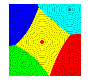
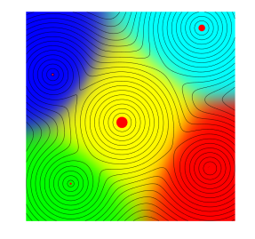
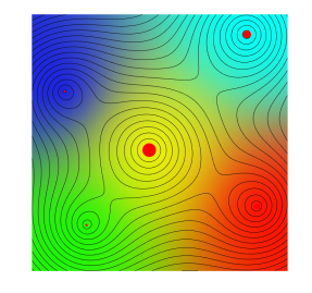
$\varepsilon=0$	$\varepsilon=0.01$	$\varepsilon=0.1$	$\varepsilon=0.3$

Fig. 1: Examples of entropic semi-discrete $\bar{c}$-transforms $\mathrm{\textbf{g}}^{\bar{c},\varepsilon}$ in 2-D, for ground cost $c(x,y)=|\!|x-y|\!|$ for varying $\varepsilon$. The black curves are the level sets of the function $\mathrm{\textbf{g}}^{\bar{c},\varepsilon}$, while the colors indicate the smoothed indicator function of the Laguerre cells $\chi_{j}^{\varepsilon}$. The red points are at locations $y_{j}\in\mathbb{R}^{2}$, and their size is proportional to $\mathrm{\textbf{g}}_{j}$.

Semi-discrete solvers

The semi-discrete case, where $\alpha$ has a density (with respect to Lebesgue measure) while $\beta=\sum_{j=1}^{m}\mathrm{\textbf{b}}_{j}\delta_{y_{j}}$ is discrete, is interesting from a computational point of view. In this setting, one can solve the problem through the lens of a variable $\mathrm{\textbf{g}}=(g(y_{j}))_{j=1}^{m}\in\mathbb{R}^{m}$, by imposing $f=g^{\bar{c},\varepsilon}$ where

$$\mathrm{\textbf{g}}^{\bar{c},\varepsilon}(x)\stackrel{{\scriptstyle\mbox{\tiny def.}}}{{=}}\left\{\begin{array}[]{l}-\varepsilon\log\sum_{j}e^{-\frac{c(x,y_{j})-\mathrm{\textbf{g}}_{j}}{\varepsilon}}\quad\text{for}\quad\varepsilon>0,\\ \min_{j}c(x,y_{j})-\mathrm{\textbf{g}}_{j}\quad\text{if}\quad\varepsilon=0.\end{array}\right.$$

The semi-dual problem then read in this semi-discrete case

$$\mathcal{L}_{c}^{\varepsilon}(\alpha,\beta)=\underset{\mathrm{\textbf{g}}\in\mathbb{R}^{m}}{\max}\;\mathcal{E}^{\varepsilon}(\mathrm{\textbf{g}})\stackrel{{\scriptstyle\mbox{\tiny def.}}}{{=}}\int_{\mathcal{X}}\mathrm{\textbf{g}}^{\bar{c},\varepsilon}(x)\mathrm{d}\alpha(x)+\sum_{j}\mathrm{\textbf{g}}_{j}\mathrm{\textbf{b}}_{j}.$$ (20)

This optimization problem is attractive because the objective function is written as an integral against measure $\alpha$, so it can be solved using stochastic gradient descent as detailed in [31]. The gradient of this functional, for any $\varepsilon\geqslant 0$ reads

$$\forall\,j\in\llbracket m\rrbracket,\quad\nabla\mathcal{E}^{\varepsilon}(\mathrm{\textbf{g}})_{j}=-\int_{\mathcal{X}}\chi_{j}^{\varepsilon}(x)\mathrm{d}\alpha(x)+\mathrm{\textbf{b}}_{j},$$ (21)

where $\chi_{j}^{\varepsilon}$ is a smoothed version of the indicator $\chi_{j}^{0}$ of the Laguerre cell $\mathbb{L}_{j}(\mathrm{\textbf{g}})$

$$\chi_{j}^{\varepsilon}(x)=\frac{e^{\frac{-c(x,y_{j})+\mathrm{\textbf{g}}_{j}}{\varepsilon}}}{\sum_{\ell}e^{\frac{-c(x,y_{\ell})+\mathrm{\textbf{g}}_{\ell}}{\varepsilon}}}.$$ (22)

In the case $\varepsilon=0$, one can introduce the Laguerre cells

$$\mathbb{L}_{j}(\mathrm{\textbf{g}})\stackrel{{\scriptstyle\mbox{\tiny def.}}}{{=}}\left\{x\in\mathcal{X}\;;\;\forall\,j^{\prime}\neq j,c(x,y_{j})-\mathrm{\textbf{g}}_{j}\leqslant c(x,y_{j^{\prime}})-\mathrm{\textbf{g}}_{j^{\prime}}\right\}$$

which induce a disjoint decomposition of $\mathcal{X}=\bigcup_{j}\mathbb{L}_{j}(\mathrm{\textbf{g}})$. When g is constant, the Laguerre cells decomposition corresponds to the Voronoi diagram partition of the space. Note that $\chi_{j}^{0}$ defined in (22) (i.e. for $\varepsilon=0$) is the indicator function of the Laguerre cell $\mathbb{L}_{j}(\mathrm{\textbf{g}})$. A simple algorithm to solve (20) is a gradient descent

$$\mathrm{\textbf{g}}^{(\ell+1)}\stackrel{{\scriptstyle\mbox{\tiny def.}}}{{=}}(1-\tau_{\ell})\mathrm{\textbf{g}}^{(\ell)}+\tau_{\ell}\int_{\mathbb{L}_{j}(\mathrm{\textbf{g}})}\mathrm{d}\alpha(x)$$ (23)

for some step size $\tau_{\ell}>0$, which only requires the computation of the Laguerre cells. In the special case $c(x,y)=|\!|x-y|\!|^{2}$, the decomposition in Laguerre cells is also known as a “power diagram”. The cells are polyhedral and can be computed efficiently using computational geometry algorithms, see [5]. The most widely used algorithm relies on the fact that the power diagram of points in $\mathbb{R}^{d}$ is equal to the projection on $\mathbb{R}^{d}$ of the convex hull of the set of points $((y_{j},|\!|y_{j}|\!|^{2}-\mathrm{\textbf{g}}_{j}))_{j=1}^{m}\subset\mathbb{R}^{d+1}$. There are numerous algorithms to compute convex hulls, for instance that of [21] in 2-D and 3-D has complexity $O(m\log(Q))$ where $Q$ is the number of vertices of the convex hull.

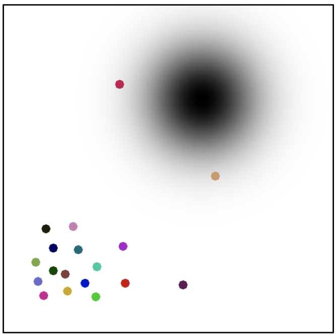
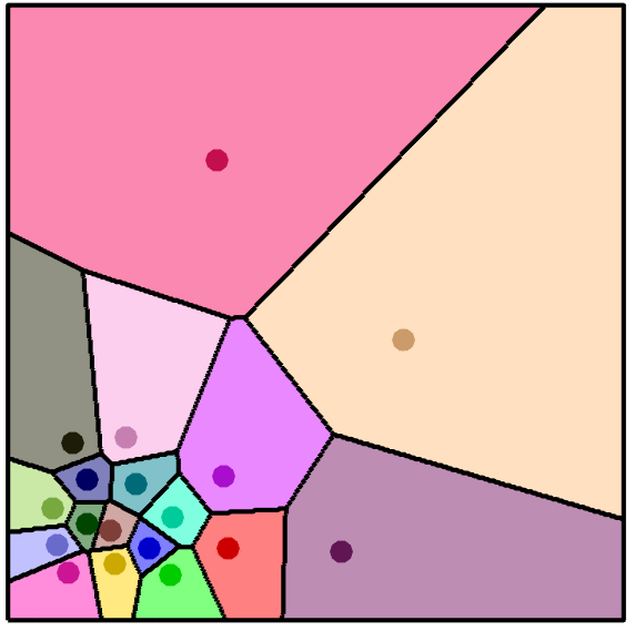
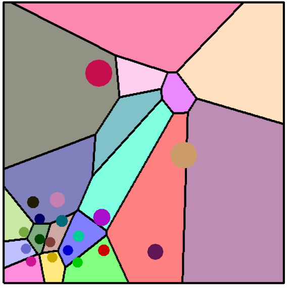
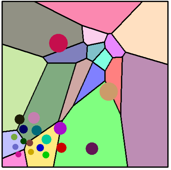
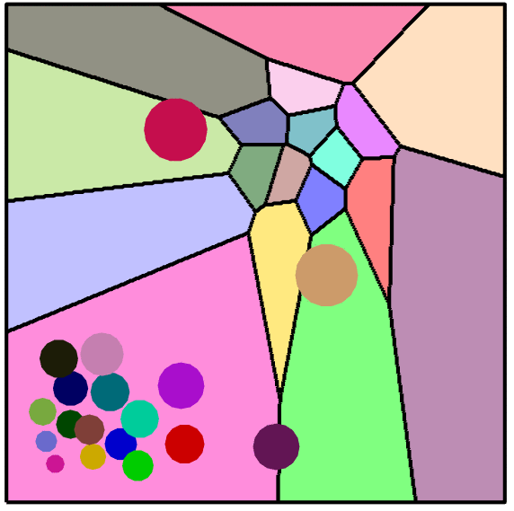
$\alpha$ and $\beta$	$\ell=1$	$\ell=20$	$\ell=40$	$\ell=100$

Fig. 2: Iterations of the gradient descent (23) to solve the semi-discrete OT (when $\varepsilon=0$). The support $(y_{j})_{j}$ of the discrete measure $\beta$ is indicated by the colored points, while the continuous measure $\alpha$ is the uniform measure on a square. The colored cells display the Laguerre partition $(\mathbb{L}_{j}(\mathrm{\textbf{g}}^{(\ell)}))_{j}$ where $\mathrm{\textbf{g}}^{(\ell)}$ is the discrete dual potential computed at iteration $\ell$.

The entropic-regularized semi-discrete formulation (20), for $\varepsilon>0$, corresponds to the minimization of a smooth functional. Indeed, one can generalize Corollary 1 to arbitrary measures (see [31]) and in particular the Hessian is upper-bounded by $1/\varepsilon$, paving the way for the use of off-the-shelf first and second order optimization methods. In practice, similarly to [42] in the un-regularized case, we advocate for the use of a quasi-Newton (L-BFGS) solver. We refer to Section 3.2 for a more detailed discussion in the case of barycenters. Note that other methods exploiting second order schemes with some regularization have been studied by [34; 59; 23; 3].

3 Smooth dual algorithms for the WBP

We now use the semi-dual formulation the Wasserstein distance detailed in Section 2.2 to solve the Wasserstein Barycenter Problem (WBP). In this section, histograms correspond to measures defined on the same space $\mathcal{X}=\mathcal{Y}$, and thus in the discrete setting, we impose $n=m$. The usual way to proceed is to take $\mathrm{\textbf{C}}_{i,j}=d(x_{i},x_{j})^{\rho}$ where $\rho\geqslant 1$ is some exponent, and $d$ is a distance on the underlying space. Then $(\mathrm{L}_{\mathrm{\textbf{C}}}^{0})^{1/\rho}$ defines the so-called (discrete) Wasserstein distance on the simplex $\Sigma_{n}$, and $(\mathcal{L}_{c}^{0})^{1/\rho}$ metrizes the weak-* convergence of measures (which corresponds to the convergence in law of random variables).

3.1 Smooth dual formulation of the WBP

Following the introduction of the WBP by [2], [27] introduced the smoothed WBP with $\varepsilon$-entropic regularization ($\varepsilon$-WBP) as

$$\underset{\mathrm{\textbf{a}}\in\Sigma_{n}}{\min}\;\sum_{k=1}^{N}w_{k}\mathrm{L}_{\mathrm{\textbf{C}}}^{\varepsilon}(\mathrm{\textbf{a}},\mathrm{\textbf{b}}_{k})=\sum_{k=1}^{N}w_{k}\mathrm{F}_{\mathrm{\textbf{b}}_{k}}(\mathrm{\textbf{a}}),$$ (24)

where $(\mathrm{\textbf{b}}_{1},\ldots,\mathrm{\textbf{b}}_{N})$ is a family of histograms in $\Sigma_{n}$ and $w\in\Sigma_{N}$ is a set of weights. When $\varepsilon=0$, the $\varepsilon$-WBP is exactly the WBP. In that case, problem (24) is in fact a linear program, as discussed later in Section 3.3. When $\varepsilon>0$ the $\varepsilon$-WBP is a strictly convex optimization problem that admits a unique solution, which can be solved with a simple gradient descent as advocated by [27]. They show that the $N$ gradients $\left[\nabla\mathrm{F}_{\mathrm{\textbf{b}}_{k}}(\mathrm{\textbf{a}})\right]_{k\leqslant N}$ can be computed at each iteration by solving $N$ Sinkhorn matrix-scaling problems. Because these gradients are themselves the result of a numerical optimization procedure, the problem of choosing a thresholds to obtain sufficient accuracy on these gradients arises. We take here a different route to solve the $\varepsilon$-WBP, which can be interpreted either as a smooth alternative to the dual WBP studied by [18] or the dual counterpart to the smoothed WBP of [27].

Theorem 2.

The barycenter $\mathrm{\textbf{a}}^{\star}$ solving (24) satisfies

$$\forall\,k=1,\ldots,N,\quad\mathrm{\textbf{a}}^{\star}=\nabla\mathrm{F}_{\mathrm{\textbf{b}}_{k}}^{*}(\mathrm{\textbf{f}}_{k}^{\star}),$$ (25)

where $(\mathrm{\textbf{f}}_{k}^{\star})_{k}$ are any solution of the smoothed dual WBP:

$$\underset{\mathrm{\textbf{f}}_{1},\ldots,\mathrm{\textbf{f}}_{N}\in\mathbb{R}^{n}}{\min}\;\sum_{k}w_{k}\mathrm{F}_{\mathrm{\textbf{b}}_{k}}^{*}(\mathrm{\textbf{f}}_{k})\quad\text{s.t.}\quad\sum_{k}w_{k}\mathrm{\textbf{f}}_{k}=0.$$ (26)

Proof.

We rewrite the barycenter problem

$$\underset{\mathrm{\textbf{a}}_{1},\ldots,\mathrm{\textbf{a}}_{N}}{\min}\;\sum_{k}w_{k}\mathrm{F}_{\mathrm{\textbf{b}}_{k}}(\mathrm{\textbf{a}}_{k})\quad\text{s.t.}\quad\mathrm{\textbf{a}}_{1}=\cdots=\mathrm{\textbf{a}}_{N}$$

whose Fenchel–Rockafelar dual reads

$$\underset{\tilde{\mathrm{\textbf{f}}}_{1},\ldots,\tilde{\mathrm{\textbf{f}}}_{N}}{\min}\;\sum_{k}w_{k}\mathrm{F}_{\mathrm{\textbf{b}}_{k}}^{*}(\tilde{\mathrm{\textbf{f}}}_{k}/w_{k})\quad\text{s.t.}\quad\sum_{k}\tilde{\mathrm{\textbf{f}}}_{k}=0.$$

Since the primal problem is strictly convex, the primal-dual relationships show that the unique solution $\mathrm{\textbf{a}}^{\star}$ of the primal can be obtained from any solution $(\tilde{\mathrm{\textbf{f}}}_{k}^{\star})_{k}$ via the relation $\mathrm{\textbf{a}}_{k}^{\star}=\nabla\mathrm{F}_{\mathrm{\textbf{b}}_{k}^{\star}}^{*}(\tilde{\mathrm{\textbf{f}}}_{k}^{\star}/w_{k})$. One obtains the desired formulation using the change of variable $\mathrm{\textbf{f}}_{k}=\tilde{\mathrm{\textbf{f}}}_{k}/w_{k}$.∎

Theorem 2 provides a simple approach to solve the $\varepsilon$-WBP: Rather than minimizing directly the sum of regularized Wasserstein distances in (24), this formulation only involves minimizing a strictly convex function with closed form objectives and gradients.

Parallel implementation

The objectives, gradients, and Hessians of the Fenchel–Legendre dual $\mathrm{F}^{*}_{\mathrm{\textbf{b}}}$ can be computed using either matrix-vector products or elementwise operations. Given $N$ histograms $(\mathrm{\textbf{b}}_{k})_{k}$ and $N$ dual variables $(\mathrm{\textbf{f}}_{k})_{k}$, the computation of $N$ objective values $(\mathrm{F}_{\mathrm{\textbf{b}}_{k}}^{*}(\mathrm{\textbf{f}}_{k}))_{k}$ and $N$ gradients $(\nabla\mathrm{F}_{\mathrm{\textbf{b}}_{k}}^{*}(\mathrm{\textbf{f}}_{k}))_{k}$ can all be vectorized. Assuming that all column vectors $\mathrm{\textbf{f}}_{k}$ and $\mathrm{\textbf{b}}_{k}$ are gathered in $n\times N$ matrices $F$ and $B$ respectively, we first define the $n\times N$ auxiliary matrices

$$A\operatorname{\overset{\operatorname{def}}{=}}e^{F/\varepsilon},\quad C\operatorname{\overset{\operatorname{def}}{=}}\frac{B}{\mathrm{\textbf{K}}A},\quad\Delta\operatorname{\overset{\operatorname{def}}{=}}A\circ(\mathrm{\textbf{K}}C)$$

to form the vector of objectives

$$H^{*}\;\operatorname{\overset{\operatorname{def}}{=}}[\mathrm{F}_{\mathrm{\textbf{b}}_{1}}^{*}(\mathrm{\textbf{f}}_{1}),\dots,\mathrm{F}_{\mathrm{\textbf{b}}_{N}}^{*}(\mathrm{\textbf{f}}_{N})]=-\varepsilon\mathds{1}_{n}^{\top}\left(B\circ\log(C)\right)$$ (27)

and the matrix of gradients

$$\nabla H^{*}\;\operatorname{\overset{\operatorname{def}}{=}}[\nabla\mathrm{F}_{\mathrm{\textbf{b}}_{1}}^{*}(\mathrm{\textbf{f}}_{1}),\dots,\nabla\mathrm{F}_{\mathrm{\textbf{b}}_{N}}^{*}(\mathrm{\textbf{f}}_{N})]=\Delta.$$ (28)

3.2 Algorithm

The $\varepsilon$-WBP in (26) has a smooth objective with respect to each of its variables $\mathrm{\textbf{f}}_{k}$, a simple linear equality constraint, and both gradients and Hessians that can be computed in closed form. We can thus compute a minimizer for that problem using a naive gradient descent outlined in Algorithm 1. Note that the iterates $F$ are projected at each iteration on the constraint $Fw=0$ (which is equivalent to projecting the gradient direction on this constraint if the initial $F$ satisfies it). To obtain a faster convergence, it is also possible to use accelerated gradient descent, quasi-Newton or truncated Newton methods [15, section 10]. In the latter case, the resulting KKT linear system is sparse, and solving it with preconjugate gradient techniques can be efficiently carried out. We omit these details and only report results using off-the-shelf L-BFGS. From the dual iterates $\mathrm{\textbf{f}}_{k}$ stored in a $n\times N$ matrix $F$, one recovers primal iterates using the formula (25), namely, $\mathrm{\textbf{a}}_{k}=e^{\mathrm{\textbf{f}}_{k}/\varepsilon}\circ\mathrm{\textbf{K}}\frac{\mathrm{\textbf{b}}_{k}}{\mathrm{\textbf{K}}e^{\mathrm{\textbf{f}}_{k}/\varepsilon}}.$ At each intermediary iteration one can thus form a solution to the smoothed Wasserstein barycenter problem by averaging these primal solutions, $\tilde{\mathrm{\textbf{a}}}=\Delta\mathds{1}_{N}/N.$ Upon convergence, these $\mathrm{\textbf{a}}_{k}$ are all equal to the unique solution $\mathrm{\textbf{a}}^{\star}$. The average at each iteration $\tilde{\mathrm{\textbf{a}}}$ converges toward that unique solution, and we use the sum of all linewise standard deviations of $\Delta$: $\mathds{1}_{d}^{\top}\sqrt{(\tilde{\Delta}\circ\tilde{\Delta})\mathds{1}_{N}/N}$, where $\tilde{\Delta}=\Delta(I_{N}-\frac{1}{N}\mathds{1}_{N}\mathds{1}_{N}^{\top})$ to monitor that convergence in our algorithms.

1:  Input: $B=[\mathrm{\textbf{b}}_{1},\ldots,\mathrm{\textbf{b}}_{N}]\in(\Sigma_{n})^{N}$, metric $M\in\mathbb{R}_{+}^{n\times n}$, barycenter weights $w\in\Sigma_{N}$, $\varepsilon>0$, tolerance $\varepsilon>0$.

2:  initialize $F\in\mathbb{R}^{n\times N}$ and form the $n\times n$ matrix $K=e^{-\mathrm{\textbf{C}}/\varepsilon}$.

3:  repeat

4:     From gradient matrix $\Delta$ (see (28)) produce update matrix $\hat{\Delta}$ using either $\Delta$ directly or other methods such as L-BFGS.

5:     $F=F-\tau\hat{\Delta}$, update with fixed step length $\tau$ or approximate line search to set $\tau$.

6:     $F=F-\frac{1}{|\!|w|\!|_{2}^{2}}(Fw)w^{\top}$  (projection such that $Gw=0$)

7:  until $\mathds{1}_{d}^{\top}\sqrt{(\tilde{\Delta}\circ\tilde{\Delta})\mathds{1}_{N}/N}<\varepsilon$, where $\tilde{\Delta}=\Delta(I_{N}-\frac{1}{N}\mathds{1}_{N}\mathds{1}_{N}^{\top})$

8:  output barycenter $\mathrm{\textbf{a}}=\Delta\mathds{1}_{N}/N$.

Algorithm 1 . Smoothed Wasserstein Barycenter, Generic Algorithm.

3.3 Smoothing and stabilization of the WBP

We make the claim in this section that smoothing the WBP is not only beneficial computationally but may also yield more stable computations. Of central importance in this discussion is the fact that the WBP can be cast as a LP of $Nn^{2}+n$ variables and $2Nn$ constraints and thus can be solved exactly for small $n$ and $N$:

$$\min_{\mathrm{\textbf{P}}_{1},\ldots,\mathrm{\textbf{P}}_{N},p} \sum_{k=1}^{N}w_{k}\langle\mathrm{\textbf{P}}_{k},\,\mathrm{\textbf{C}}\rangle$$ (29)

s.t. $$\mathrm{\textbf{P}}_{k}\in\mathbb{R}^{n\times n}_{+}\ \forall k\leqslant N;\mathrm{\textbf{a}}\in\Sigma_{n},$$

$$\mathrm{\textbf{P}}_{k}^{\top}\mathds{1}_{n}=\mathrm{\textbf{b}}_{k}\ \forall k\leqslant N,$$

$$\mathrm{\textbf{P}}_{1}\mathds{1}_{n}=\dots=\mathrm{\textbf{P}}_{N}\mathds{1}_{n}=\mathrm{\textbf{a}}.$$

Given couplings $\mathrm{\textbf{P}}_{1}^{\star},\ldots,\mathrm{\textbf{P}}_{N}^{\star}$ which are optimal solutions to (29), the solution to the WBP is equal to the marginal common to all those couplings: $\mathrm{\textbf{a}}^{\star}=\mathrm{\textbf{P}}_{k}^{\star}\mathds{1}_{n}$ for any $k\leqslant N$. For small $N$ and $n$, this problem is tractable, but it can be quite ill-posed as we see next.

Indeed, it is known that the $2$-Wasserstein mean of two univariate (continuous) Gaussian densities of mean and standard deviation $(\mu_{1},\sigma_{1})$ and $(\mu_{2},\sigma_{2})$, respectively, is a Gaussian of mean $(\mu_{1}+\mu_{2})/2$ and standard deviation $(\sigma_{1}+\sigma_{2})/2$ [2, section 6.3]. This fact is illustrated in the top left plot of Figure 3, where we display the Wasserstein average $\mathcal{N}(0,5/8)$ of the two densities $\mathcal{N}(2,1)$ and $\mathcal{N}(-2,1/4)$. That plot is obtained by using smoothed spline interpolations of a uniformly spaced grid of $100$ values, as can be better observed in the top-right (stair) plot, where the discrete evaluations of these densities are respectively denoted $\mathrm{\textbf{a}}_{W}$, $\mathrm{\textbf{b}}_{1}$, and $\mathrm{\textbf{b}}_{2}$.

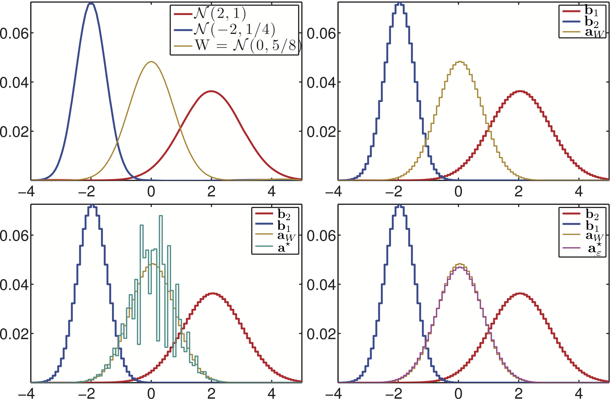
Fig. 3: Top left: two Gaussian densities and their barycenter. Top right: same densities, discretized. Bottom left: discretization of the true barycenter vs. the optimum of (29). Bottom right: barycenter computed with our smoothing approach.

Naturally, one would expect the barycenter of $\mathrm{\textbf{b}}_{1}$ and $\mathrm{\textbf{b}}_{2}$ to be close, in some sense, to the discretized histogram $\mathrm{\textbf{a}}_{W}$ of their true barycenter. Histogram $\mathrm{\textbf{a}}^{\star}$, displayed in the bottom-left plot, is the exact optimal solution of (29), computed with the simplex method. That WBP reduces to a linear program of $2\times 100^{2}$ variables and $300$ constraints. We observe that $W_{2}^{2}(\mathrm{\textbf{a}}^{\star},\mathrm{\textbf{b}}_{1})+W_{2}^{2}(\mathrm{\textbf{a}}^{\star},\mathrm{\textbf{b}}_{2})=0.5833950$ whereas $W_{2}^{2}(\mathrm{\textbf{a}}_{W},\mathrm{\textbf{b}}_{1})+W_{2}^{2}(\mathrm{\textbf{a}}_{W},\mathrm{\textbf{b}}_{2})=0.5834070$. The solution obtained with the network simplex has, indeed, a smaller objective than the discretized version of the true barycenter.

The bottom right plot displays the solution of the smoothed WBP (with smoothing parameter $\varepsilon=\frac{1}{100}$ and a ground cost C that has been rescaled to have a median value of $1$). The objective value for that smoothed approximation is $0.5834597$.

This numerical experiment does not contradict the fact that the discretized barycenter $\mathrm{\textbf{a}}^{\star}$ converges (in the weak* sense) to the continuous barycenter as the grid size tends to zero, as shown in [18]. This observation illustrates however that, because it is defined as the $\operatorname{argmin}$ of a linear program, the true Wasserstein barycenter may be unstable (when viewed as an histogram, and not in the sense of the weak* topology of measures), even for such a simple problem and for large $n$ as illustrated in Figure 4. Regularizing the Wasserstein distances thus has the added benefit of smoothing the resulting solution of the WBP and that of mitigating low sample size effects.

The choice of the parameter $\varepsilon$ is application-dependent, but it should scale with the typical distance between sampling locations (e.g., the grid step size). Note that choosing too small $\varepsilon$ not only leads to slower convergence of our algorithm but also leads to numerical instabilities and can ultimately break the convergence. In simple settings such as low-dimensional grids, computational strategies can overcome some of these issues [53].

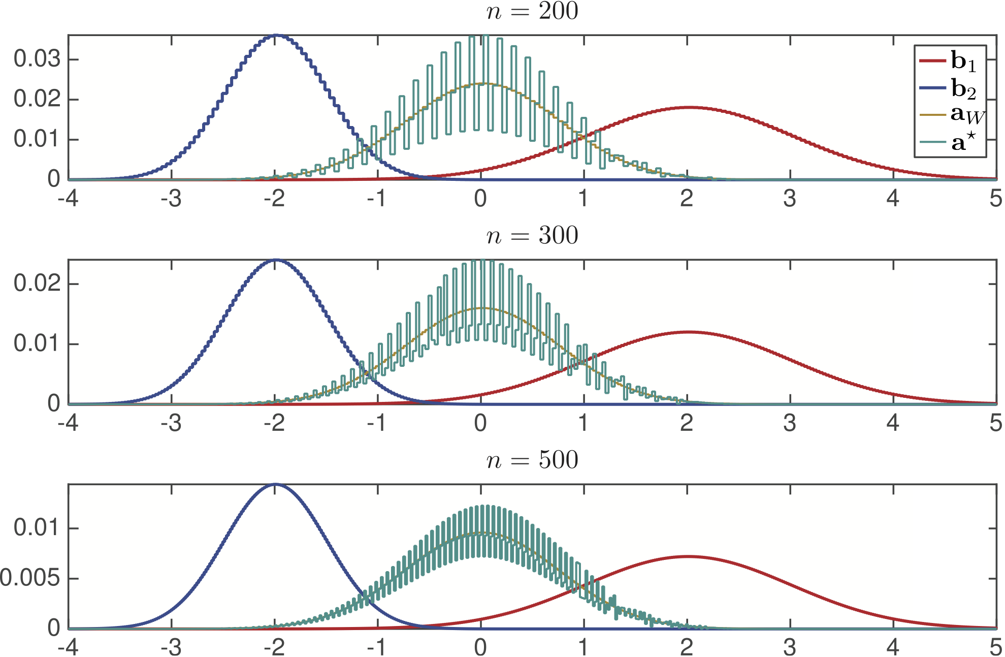
Fig. 4: Plots of the exact barycenters for varying grid size $n$.

3.4 Performance on the WBP

We compare in this section the behavior of the smooth dual approach presented in this paper with that of (i) the smooth primal approach of [27], (ii) the dual approach of [18], and (iii) the Bregman iterative projections approach of [10]. We compare these methods on the simple task of computing the Wasserstein barycenter of $12$ histograms laid out on the $100\times 100$ grid, as previously introduced in [10, section 3.2]. We outline briefly all four methods below and follow by presenting numerical results.

Smooth primal first order descent

Cuturi and Doucet [27, section 5] proposed to directly minimize (24) with a regularizer $\varepsilon>0$. That objective can be evaluated by running $N$ Sinkhorn fixed-point iterations in parallel. That objective is differentiable, and its gradient is equal to $\varepsilon\sum_{k}w_{k}\log\mathrm{\textbf{u}}_{k}$, where the $\mathrm{\textbf{u}}_{k}$ are the left scalings obtained with that subroutine. A weakness of that approach is that a tolerance $\varepsilon$ for the Sinkhorn fixed-point algorithm must be chosen. Convergence for the Sinkhorn algorithm can be measured with a difference in $\ell_{1}$ norm (or any other norm) between the row and column marginals of $\mathop{\operator@font diag}\nolimits(\mathrm{\textbf{u}}_{k})e^{-\mathrm{\textbf{C}}/\varepsilon}\mathop{\operator@font diag}\nolimits(\mathrm{\textbf{v}}_{k})$ and the targeted histograms a and $\mathrm{\textbf{b}}_{k}$. Setting that tolerance $\varepsilon$ to a large value ensures a faster convergence of the subroutine but would result in noisy gradients which could slow the convergence of the algorithm. Because the smoothed dual approach only relies on closed form expressions, we do not have to take into account such a trade-off.

Iterative Bregman projections

Benamou et al. [10, Proposition 1] recall that the computation of the smoothed Wasserstein distance between $\mathrm{\textbf{a}},\mathrm{\textbf{b}}$ using the Sinkhorn algorithm can be interpreted as an iterative alternated projection of the $n\times n$ kernel matrix $e^{-\mathrm{\textbf{C}}/\varepsilon}$ onto two affine sets, $\left\{\mathrm{\textbf{P}}\;;\;\mathrm{\textbf{P}}\mathds{1}_{n}=\mathrm{\textbf{a}}\right\}$ and $\left\{\mathrm{\textbf{P}}\;;\;\mathrm{\textbf{P}}^{\top}\mathds{1}_{n}=\mathrm{\textbf{b}}\right\}$. That projection is understood to be in the Kullack–Leibler divergence sense. More interestingly, the authors also show that the smoothed WBP itself can also be tackled using an iterative alternated projection, cast this time in a space of dimension $n\times n\times N$. Very much like the original Sinkhorn algorithm, these projections can be computed for a cheap price, by only tracking variables of size $n\times N$. This approach yields an extremely simple, parameter-free generalization of the Sinkhorn algorithm which can be applied to the WBP.

Smooth dual L-BFGS

The dual formulation with variables $(\mathrm{\textbf{f}}_{1},\ldots,\mathrm{\textbf{f}}_{N})\in(\mathbb{R}^{n})^{N}$ of (26) can be solved using a constrained L-BFGS solver At each iteration of that minimization, we can recover a feasible solution a to the primal problem of (24) via the primal-dual relation $\mathrm{\textbf{a}}=\frac{1}{N}\sum_{k}\nabla\mathrm{F}_{\mathrm{\textbf{b}}_{k}}^{*}(\tilde{\mathrm{\textbf{f}}}_{k})$.

Dual $(\varepsilon=0)$ with L-BFGS

This approach amounts to solving directly the (nondifferentiable) dual problem described in (26) with no regularization, namely, $\varepsilon=0$. Subgradients for the Fenchel–Legendre transforms $\mathrm{F}_{\mathrm{\textbf{b}}_{k}}^{*}$ can be obtained in closed form as detailed in [18]. As with the smoothed-dual formulation, we can also obtain a feasible primal solution by averaging subgradients. We follow the recommendation of [18] to use L-BFGS. The nonsmoothness of that energy is challenging: we have observed empirically that a naive subgradient method applied to that problem fails to converge in all examples we have considered, whereas the L-BFGS approach converges, albeit without guarantees.

Averaging truncated mixtures of Gaussians

We consider the 12 truncated mixtures of Gaussians introduced in [10, section 3.2]. To compare computational time, we use $Nn^{2}$ elementary operations as the computation unit. These $Nn^{2}$ operations correspond to matrix-matrix products in the smoothed Wasserstein case and $Nn$ computations of nearest neighbor assignments among $n$ possible neighbors. Note that in both cases (Gaussian matrix product and nearest neighbors under the $\ell_{2}$ metric) computations can be accelerated by considering fast Gaussian convolutions and $kd$-trees for fast nearest neighbor search. We do not consider them in this section. We plot in Figure 5 the optimality gap with respect to the optimum of these four techniques as a function of the number of computations, by taking as a reference the lowest value attained across all methods. This value is attained, as in [10], by the iterative Bregman projections approach after 771 iterations (not displayed in our graph). We show these gaps for both the smoothed $(\varepsilon=1/100)$ and nonsmoothed objectives $(\varepsilon=0)$. We observe that the iterative Bregman approach outperforms all other techniques. The smoothed-dual approach follows closely, and its performance is significantly improved when using the heuristic initialization technic detailed in [28].

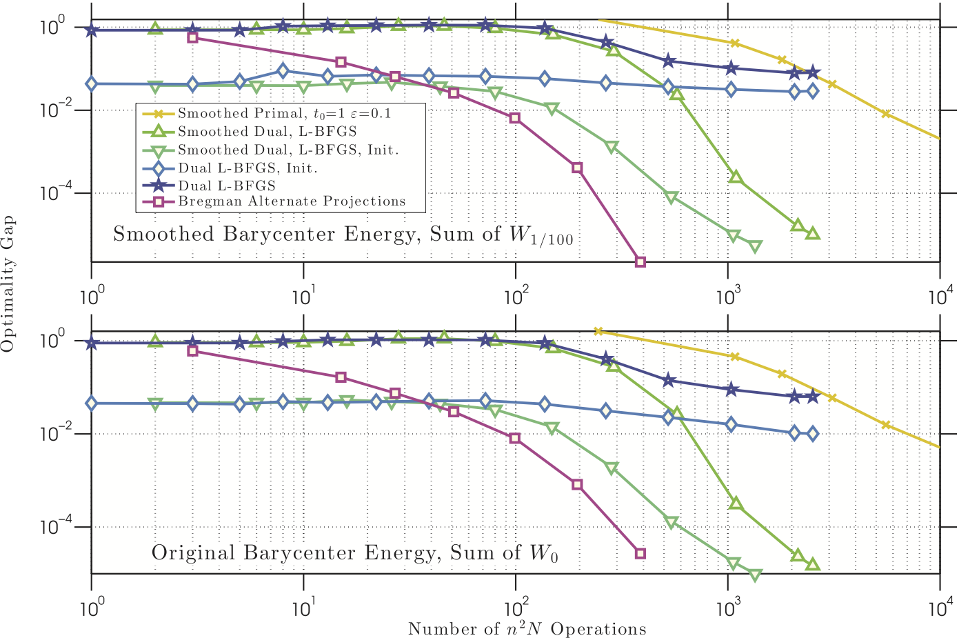
Fig. 5: Number of quadratic operations (matrix vector product or min search in a matrix) vs. optimization gap to the smallest possible objective found after running $10^{5}$ iterations of all algorithms, log-log scale. Because the smooth primal/dual approaches optimize a different criterion than the dual approach, we plot both objectives. The Smooth dual L-BFGS converges faster in both smooth and non-smooth metrics. Note the impact of the initialization detailed in [28].

4 Regularized problems

We show in this section that our dual optimization framework is versatile enough to deal with functionals involving Wasserstein distances that are more general than the initial WBP problem.

4.1 Regularized Wasserstein barycenters

In order to enforce additional properties of the barycenters, it is possible to penalize (24) with an additional convex regularization, and consider

$$\underset{\mathrm{\textbf{a}}}{\min}\;\sum_{k=1}^{N}w_{k}\mathrm{F}_{\mathrm{\textbf{b}}_{k}}(\mathrm{\textbf{a}})+J(\mathcal{A}\mathrm{\textbf{a}}),$$ (30)

where $J$ is a convex real-valued function, and $\mathcal{A}$ is a linear operator.

The following proposition shows how to compute such a regularized barycenter through a dual optimization problem.

Proposition 3.

The dual problem to (30) reads

$$\underset{(\mathrm{\textbf{f}}_{k})_{k=1}^{N},\mathrm{\textbf{g}}}{\min}\;\sum_{k=1}^{N}w_{k}\mathrm{F}_{\mathrm{\textbf{b}}_{k}}^{*}(\mathrm{\textbf{f}}_{k})+J^{*}(\mathrm{\textbf{g}})+\iota_{H}((\mathrm{\textbf{f}}_{k})_{k},\mathrm{\textbf{g}}),$$ (31)

$$\quad\text{where}\quad H\stackrel{{\scriptstyle\mbox{\tiny def.}}}{{=}}\left\{((\mathrm{\textbf{f}}_{k})_{k=1}^{N},\mathrm{\textbf{g}})\;;\;\mathcal{A}^{*}\mathrm{\textbf{g}}+\sum_{k}w_{k}\mathrm{\textbf{f}}_{k}=0\right\},$$

and the primal-dual relationships read

$$\forall\,k=1,\ldots,N,\quad\mathrm{\textbf{a}}=\nabla\mathrm{F}_{\mathrm{\textbf{b}}_{k}}^{*}(\mathrm{\textbf{f}}_{k}).$$ (32)

Proof.

We rewrite the initial program (30) as

$$\underset{\pi}{\min}\;F(B\pi)+G(\pi),$$ (33)

where we denoted, for $\pi=(\mathrm{\textbf{a}},\mathrm{\textbf{a}}_{1},\ldots,\mathrm{\textbf{a}}_{N})$,

$$B\pi \stackrel{{\scriptstyle\mbox{\tiny def.}}}{{=}}(\mathcal{A}\mathrm{\textbf{a}},\mathrm{\textbf{a}},\mathrm{\textbf{a}}_{1},\ldots,\mathrm{\textbf{a}}_{N}),$$

$$F(\beta,\mathrm{\textbf{b}},\mathrm{\textbf{a}}_{1},\ldots,\mathrm{\textbf{a}}_{N}) \stackrel{{\scriptstyle\mbox{\tiny def.}}}{{=}}J(\beta)+\iota_{C}(\mathrm{\textbf{b}},\mathrm{\textbf{a}}_{1},\ldots,\mathrm{\textbf{a}}_{N}),$$

$$G(\mathrm{\textbf{a}},\mathrm{\textbf{a}}_{1},\ldots,\mathrm{\textbf{a}}_{N}) \stackrel{{\scriptstyle\mbox{\tiny def.}}}{{=}}\sum_{k}w_{k}\mathrm{F}_{\mathrm{\textbf{b}}_{k}}(\mathrm{\textbf{a}}_{k})$$

for $C\stackrel{{\scriptstyle\mbox{\tiny def.}}}{{=}}\left\{(\mathrm{\textbf{b}},\mathrm{\textbf{a}}_{1},\ldots,\mathrm{\textbf{a}}_{N})\;;\;\forall k,\mathrm{\textbf{a}}_{k}=\mathrm{\textbf{b}}\right\}$. The Fenchel–Rockafelear dual to (33) reads

$$\underset{\nu=\{\mathrm{\textbf{g}},\mathrm{\textbf{f}},(\mathrm{\textbf{f}}_{k})_{k}\}}{\max}\;-F^{*}(\nu)-G^{*}(-B^{*}\nu),$$

where

$$G^{*}(\mathrm{\textbf{f}},\mathrm{\textbf{f}}_{1},\ldots,\mathrm{\textbf{f}}_{N}) =\sum_{k}w_{k}\mathrm{F}_{\mathrm{\textbf{b}}_{k}}^{*}(\mathrm{\textbf{f}}_{k}/w_{k})+\iota_{\{0\}}(\mathrm{\textbf{f}}),$$

$$B^{*}(\nu) =(\mathcal{A}^{*}\mathrm{\textbf{g}}+\mathrm{\textbf{f}},\mathrm{\textbf{f}}_{1},\ldots,\mathrm{\textbf{f}}_{N}),$$

$$F^{*}(\nu) =J^{*}(\mathrm{\textbf{g}})+\iota_{C^{\bot}}(\mathrm{\textbf{f}},\mathrm{\textbf{f}}_{1},\ldots,\mathrm{\textbf{f}}_{N}),$$

where $C^{\bot}=\left\{(\mathrm{\textbf{f}},\mathrm{\textbf{f}}_{1},\ldots,\mathrm{\textbf{f}}_{N})\;;\;\mathrm{\textbf{f}}+\sum_{k}\mathrm{\textbf{f}}_{k}=0\right\}$. One thus obtains the dual

$$\underset{\mathrm{\textbf{g}},b,(\mathrm{\textbf{f}}_{k})_{k}}{\min}\;\sum_{k}w_{k}\mathrm{F}_{\mathrm{\textbf{b}}_{k}}^{*}(-\mathrm{\textbf{f}}_{k}/w_{k})+J^{*}(\mathrm{\textbf{g}})\quad\text{s.t.}\quad\left\{\begin{array}[]{l}\mathcal{A}^{*}\mathrm{\textbf{g}}+\mathrm{\textbf{f}}=0,\\ \mathrm{\textbf{f}}+\sum_{k}\mathrm{\textbf{f}}_{k}=0.\end{array}\right.$$

The primal-dual relationships reads $\pi\in\partial G^{*}(-B^{*}\nu)$, and hence (32). Changing $-\mathrm{\textbf{f}}_{k}/w_{k}$ into $\mathrm{\textbf{f}}_{k}$ gives the desired formula.  ∎

Relevant examples of penalizations $J$ include the following:

• In order to enforce some spread of the barycenter, one can use $\mathcal{A}=\mathrm{Id}$ and $J(\mathrm{\textbf{a}})=\frac{\lambda}{2}|\!|\mathrm{\textbf{a}}|\!|^{2}$, in which case $J^{*}(\mathrm{\textbf{f}})=\frac{1}{2\lambda}|\!|\mathrm{\textbf{f}}|\!|^{2}$. In contrast to (26), the dual problem (31) is equivalent to an unconstraint smooth optimization. This problem can be solved using a simple Newton descent.

• One can also enforce that the barycenter entries are smaller than some maximum value $\rho$ by setting $\mathcal{A}=\mathrm{Id}$ and $J=\iota_{\mathcal{C}}$, where $\mathcal{C}=\left\{\mathrm{\textbf{a}}\;;\;|\!|\mathrm{\textbf{a}}|\!|_{\infty}\leqslant\rho\right\}$. In this case, one has $J^{*}(\mathrm{\textbf{f}})=\rho|\!|\mathrm{\textbf{f}}|\!|_{1}$. The optimization (31) is equivalent an unconstrained nonsmooth optimization. Since the penalization is an $\ell^{1}$ norm, one solves it using first order proximal methods as detailed in section 4.2 bellow.

• To force the barycenter to assume some fixed values $\mathrm{\textbf{a}}_{I}^{0}\in\mathbb{R}^{|I|}$ on a given set $I$ of indices, one can use $\mathcal{A}=\mathrm{Id}$ and $J=\iota_{\mathcal{C}}$, where $\mathcal{C}=\left\{\mathrm{\textbf{a}}\;;\;\mathrm{\textbf{a}}_{I}=\mathrm{\textbf{a}}_{I}^{0}\right\}$, where $\mathrm{\textbf{a}}_{I}=(\mathrm{\textbf{a}}_{i})_{i\in I}$. One then has $J^{*}(\mathrm{\textbf{f}})=\langle\mathrm{\textbf{f}}_{I},\,\mathrm{\textbf{a}}_{I}^{0}\rangle+\iota_{\{0\}}(\mathrm{\textbf{f}}_{I^{c}})$.

• To force the barycenter to have some smoothness, one can select $\mathcal{A}$ to be a spacial derivative operator (for instance, a gradient approximated on some grid or mesh) and $J$ to be a norm such as an $\ell^{2}$ norm (to ensure uniform smoothness) or an $\ell^{1}$ norm (to ensure piecewise regularity). We explore this idea in Section 4.3.

4.2 Resolution using first order proximal splitting

Assuming without loss of generality that $w_{N}\neq 0$ (otherwise one simply needs to permute the ordering of the input densities), one can note that it is possible to remove $\mathrm{\textbf{f}}_{N}$ from (31) by imposing

$$\mathrm{\textbf{f}}_{N}\stackrel{{\scriptstyle\mbox{\tiny def.}}}{{=}}-\frac{\mathcal{A}^{*}\mathrm{\textbf{g}}}{w_{N}}-\sum_{i=1}^{N-1}\frac{w_{k}}{w_{N}}\mathrm{\textbf{f}}_{k},$$

and denoting $x\stackrel{{\scriptstyle\mbox{\tiny def.}}}{{=}}((\mathrm{\textbf{f}}_{k})_{k=1}^{N-1},\mathrm{\textbf{g}})$, one can consider the following optimization problem without the $H$ constraint

$$\underset{x}{\min}\;F(x)+G(x)\quad\text{where}\quad\left\{\begin{array}[]{l}F(x)\stackrel{{\scriptstyle\mbox{\tiny def.}}}{{=}}\sum_{k=1}^{N-1}w_{k}\mathrm{F}_{\mathrm{\textbf{b}}_{k}}^{*}(\mathrm{\textbf{f}}_{k})+w_{N}\mathrm{F}_{\mathrm{\textbf{b}}_{N}}^{*}\left(\mathrm{\textbf{f}}_{N}(x)\right),\\ G(x)\stackrel{{\scriptstyle\mbox{\tiny def.}}}{{=}}J^{*}(\mathrm{\textbf{g}}).\end{array}\right.$$ (34)

We assume that one is able to compute the proximal operator of $J^{*}$

$$\operatorname{Prox}_{\tau J^{*}}(\mathrm{\textbf{g}})\stackrel{{\scriptstyle\mbox{\tiny def.}}}{{=}}\underset{\mathrm{\textbf{g}}^{\prime}}{\operatorname{argmin}}\;\frac{1}{2}|\!|\mathrm{\textbf{g}}-\mathrm{\textbf{g}}^{\prime}|\!|^{2}+\tau J^{*}(\mathrm{\textbf{g}}^{\prime}).$$ (35)

It is, for instance, an orthogonal projector on a convex set $C$ when $J^{*}=\iota_{C}$ is the indicator of $C$. One can easily compute this projection, for instance, when $J$ is the $\ell^{2}$ or the $\ell^{1}$ norm (see Section 4.3). We refer to [8] for more background on proximal operators.

The proximal operator of $G$ is then simply

$$\forall\,x=((\mathrm{\textbf{f}}_{k})_{k=1}^{N-1},\mathrm{\textbf{g}}),\quad\operatorname{Prox}_{\tau G}(x)=((\mathrm{\textbf{f}}_{k})_{k=1}^{N-1},\operatorname{Prox}_{\tau J^{*}}(\mathrm{\textbf{g}})).$$

Note also that the function $F$ is smooth with a Lipschitz gradient and that

$$\nabla F((\mathrm{\textbf{f}}_{k})_{k=1}^{N-1},\mathrm{\textbf{g}})=\left((w_{k}(\nabla\mathrm{F}_{\mathrm{\textbf{b}}_{k}}^{*}(\mathrm{\textbf{f}}_{k})-\nabla\mathrm{F}_{\mathrm{\textbf{b}}_{N}}^{*}(\mathrm{\textbf{f}}_{N})))_{k=1}^{N-1},-\mathcal{A}\nabla\mathrm{F}_{\mathrm{\textbf{b}}_{N}}^{*}(\mathrm{\textbf{f}}_{N})\right).$$

The simplest algorithm to solve (34) is the forward-backward algorithm, whose iteration reads

$$x^{(\ell+1)}=\operatorname{Prox}_{\tau J^{*}}\left(x^{(\ell)}-\tau\nabla F(x^{(\ell)})\right).$$ (36)

If $0<\tau<2/L$ where $L$ is the Lipschitz constant of $\nabla F$, then $x^{(\ell)}$ converge to a solution of (34); see [8] and the references therein. In order to accelerate the convergence of the method, one can use accelerated schemes such as FISTA’s algorithm [9].

4.3 Total variation regularization

A typical example of regularization to enforce some geometrical regularity in the barycenter is the total variation regularization on a grid in $\mathbb{R}^{d}$ (e.g., $d=2$ for images). It is obtained by considering

$$\mathcal{A}\mathrm{\textbf{a}}\stackrel{{\scriptstyle\mbox{\tiny def.}}}{{=}}\nabla\mathrm{\textbf{a}}=(\nabla_{i}\mathrm{\textbf{a}})_{i}\quad\text{and}\quad J(\mathrm{\textbf{f}})\stackrel{{\scriptstyle\mbox{\tiny def.}}}{{=}}\lambda\sum_{i}|\!|\mathrm{\textbf{f}}_{i}|\!|_{\beta},$$ (37)

where $\nabla_{i}\mathrm{\textbf{a}}\in\mathbb{R}^{d}$ is a finite difference approximation of the gradient at a point indexed by $i$, and $\lambda\geqslant 0$ is the regularization strength. When using the $\ell^{2}$ norm to measure the gradient amplitude, i.e., $\beta=2$, one obtains the so-called isotropic total variation, which tends to round corners and essentially penalizes the length of the level sets of the barycenter, possibly merging clusters together. When using instead the $\ell^{1}$ norm, i.e., $\beta=1$, one obtains the so-called anisotropic total variation, which penalizes independently horizontal and vertical derivative, thus favoring the emergence of axis-aligned edges and giving a “crystalline” look to the barycenters. We refer, for instance, to [19] for a study of the effect of TV regularization on the shapes of levelsets using isotropic and crystalline total variations.

In this case, it is possible to compute in closed form the proximal operator (35). Indeed, one has $J^{*}=\iota_{|\!|\cdot|\!|_{\beta^{*}}\leqslant\lambda}$, where $\beta^{*}$ is the conjugate exponent $1/\beta+1/\beta^{*}=1$. One can compute explicitly the proximal operator in the case $\beta\in\{1,2\}$ since they correspond to orthogonal projectors on $\ell^{\beta^{*}}$ balls

$$\operatorname{Prox}_{\tau J^{*}}(\mathrm{\textbf{g}})_{i}=\left\{\begin{array}[]{l}\min(\max(\mathrm{\textbf{g}}_{i},-\lambda),\lambda)\quad\text{if}\quad\beta=1,\\ \mathrm{\textbf{g}}_{i}\frac{\lambda}{\max(|\!|\mathrm{\textbf{g}}_{i}|\!|,1)}\quad\text{if}\quad\beta=2.\end{array}\right.$$

4.4 Barycenters of images

We start by computing barycenters of a small number of two-dimensional (2-D) images that are discretized on an uniform rectangular grid of $n=256\times 256$ pixels $(z_{i})_{i=1}^{N}$ of $[0,1]^{2}$. The entropic regularization parameter is set to $\varepsilon=1/n$. We use either the isotropic ($\beta=2$) or anisotropic ($\beta=1$) total variation presented above, where $\nabla$ is defined using standard forward finite differences along each axis and using Neumann boundary conditions. The metric is the usual squared Euclidean metric

$$\forall\,(i,j)\in\{1,\ldots,n\}^{2},\quad\mathrm{\textbf{C}}_{i,j}=|\!|z_{i}-z_{j}|\!|^{2}.$$ (38)

The Gibbs kernel $\mathrm{\textbf{K}}=e^{-\mathrm{\textbf{C}}/\varepsilon}$ is a filtering with a Gaussian kernel that can be applied efficiently to histograms in nearly linear time; see [57] for more details about convolutional kernels.

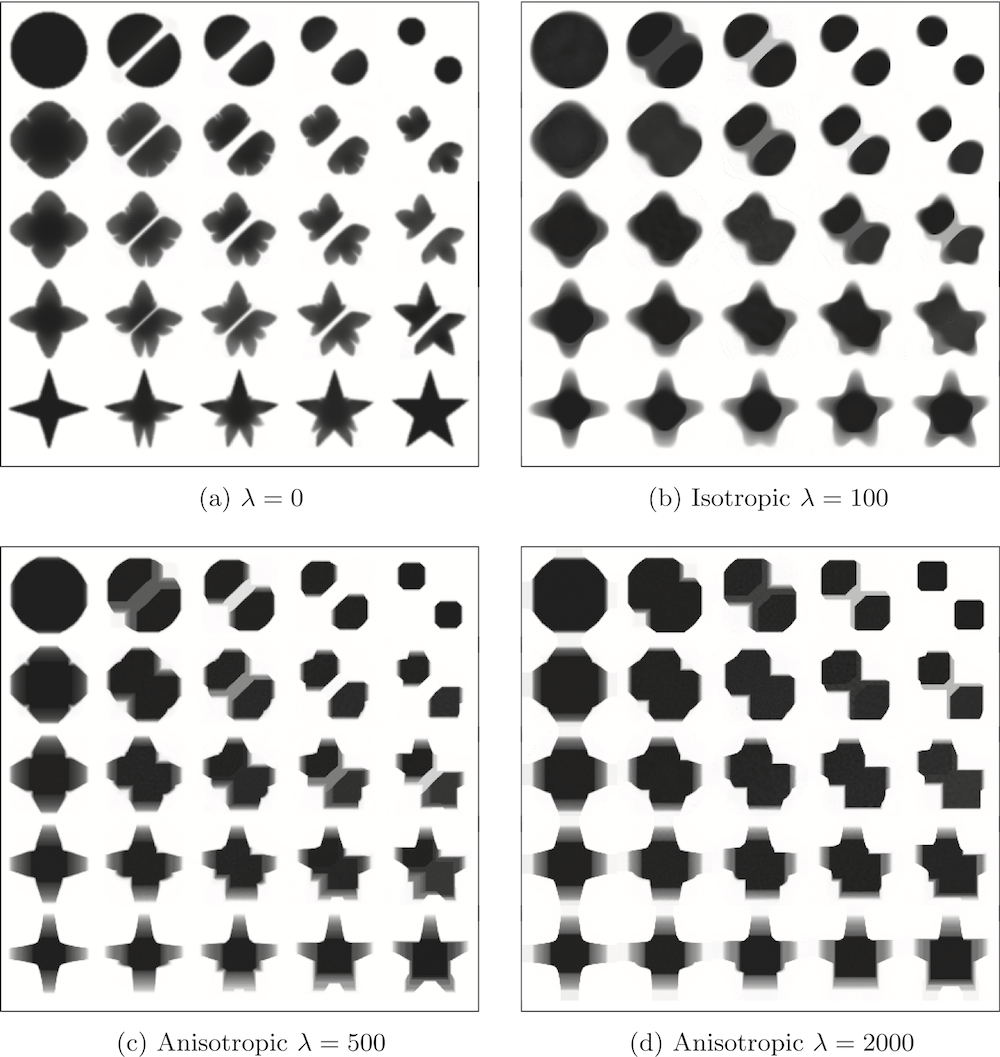
Fig. 6: Examples of isotropic and anisotropic TV regularization for the computation of barycenters between four input densities. The weights $(w_{k})_{k=1}^{N}$ are bilinear interpolation weights, so that it is, for instance, $w=(1,0,0,0)$ on the top left corner and $(0,0,0,1)$ on the bottom right corner.

Figure 6 shows examples of barycenters of $N=4$ input histograms computed by solving (30) using the projected gradient descent method (36). The input histograms represent 2-D shapes and are uniform (constant) distributions inside the support of the shapes. Note that in general the barycenters are not shapes, i.e., they are not uniform distributions, but this method can nevertheless be used to define meaningful averaging of shapes as exposed in [57]. Figure 6 compares the effects of $\beta\in\{1,2\}$, and one can clearly see how the isotropic total variation ($\beta=2$) rounds the corners of the input densities, while the anisotropic version ($\beta=1$) favors horizontal/vertical edges.

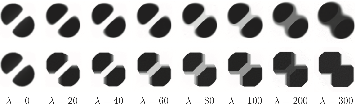
Fig. 7: Influence of $\lambda$ parameter for the iso-barycenter (i.e., $w=(1/2,1/2)$) between two input densities. (They are the upper left and upper right corner of the $\lambda=0$ case in Figure 6.) Top row: isotropic total variation $(\beta=2)$. Bottom row: anisotropic total variation $(\beta=1)$.

Figure 7 shows the influence of the regularization strength $\lambda$ to compute the iso-barycenter of $N=2$ shapes. This highlights the fact that this total variation regularization has the tendency to group together small clusters, which might be beneficial for some applications, as illustrated in Section 4.5 on magnetoencephalography (MEG) data denoising.

4.5 Barycenters of MEG data

We applied our method to an MEG dataset. In this setup, the brain activity of a subject is recorded (Elekta Neuromag, 306 sensors of which 204 planar gradiometers and 102 magnetometers, sampling frequency 1000Hz) while the subject reacted to the presentation of a target stimulus by pressing either the left or the right button.

Data is preprocessed applying signal space separation correction, interpolation of noisy sensors, and realignment of data into a subject-specific head position (MaxFilter, Elekta Neuromag). The signal was then filtered (low pass 40HZ), and artifacts such as blinks and heartbeats were removed thanks to signal-space projection using the Brainstorm software. The samples we used for our barycenter computations are an average of the norm of the two gradiometers for each channel from stimulation onto 50ms, and the classes were the left or right button.

This results in two classes of recordings, one for each pressed button. We aim at computing a representative activity map for each class using Wasserstein barycenters. For each class we have $N=33$ recordings $(\mathrm{\textbf{b}}_{k})_{k=1}^{N}$ each having $n=66$ samples located on the vertices of an hexahedral mesh of a hemisphere (corresponding to a MEG recording helmet). These recorded values are positive by construction, and we rescale them linearly to impose $\mathrm{\textbf{b}}_{k}\in\Sigma_{n}$. Figure 8, top row, shows some samples from this dataset, displayed using interpolated colors as well as iso-level curves. The black dots represent the position $(z_{i})_{i=1}^{n}$ of the electrodes on the half-sphere of the helmet, flattened on a 2-D disk.

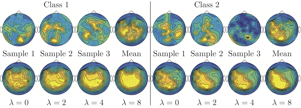
Fig. 8: Barycenter computation on MEG data. The left/right panels show, respectively, the first and the second class, corresponding to recordings where the subject is asked to push the left or the right button. Top row: examples of input histograms $\mathrm{\textbf{b}}_{k}$ for each class, as well as the $\ell^{2}$ mean $N^{-1}\sum_{k}\mathrm{\textbf{b}}_{k}$. Bottom row: computed TV-regularized barycenter for different values of $\lambda$ ($\lambda=0$ corresponding to no regularization).

We computed TV-regularized barycenters independently for each class by solving (30) with the TV regularization using the projected gradient descent method (36). We used a squared Euclidean metric (38) on the flattened hemisphere. Since the data is defined on an irregular graph, instead of (37), we use a graph-based discrete gradient. We denote $((i,j))_{(i,j)\in\mathcal{G}}$ the graph which connects neighboring electrodes. The gradient operator on the graph is

$$\forall\,\mathrm{\textbf{a}}\in\mathbb{R}^{n},\quad\mathcal{A}\mathrm{\textbf{a}}\stackrel{{\scriptstyle\mbox{\tiny def.}}}{{=}}(\mathrm{\textbf{a}}_{i}-\mathrm{\textbf{a}}_{j})_{(i,j)\in\mathcal{G}}\in\mathbb{R}^{|\mathcal{G}|}.$$

The total variation on this graph is then obtained by using $J=\lambda|\!|\cdot|\!|_{1}$, the $\ell^{1}$ norm, i.e., we use $\beta=1$ in (37).

Figure 8 compares the naive $\ell^{2}$ barycenters (i.e., the usual mean), barycenters obtained without regularization (i.e., $\lambda=0$), and barycenters computed with an increasing regularization strength $\lambda$. The input histograms $(\mathrm{\textbf{a}}_{k})_{k}$ being very noisy, the use of regularization is important to make the area of significant activity emerge from the noise. The use of a TV regularization helps to keep a sharp transition between active and nonactive regions.

4.6 Gradient flow

Instead of computing barycenters, we now use our regularization to define time-evolutions, which are defined through a so-called discrete gradient flow.

Starting from an initial histogram $\mathrm{\textbf{a}}_{0}\in\Sigma_{n}$, we define iteratively

$$\mathrm{\textbf{a}}_{k+1}\stackrel{{\scriptstyle\mbox{\tiny def.}}}{{=}}\underset{\mathrm{\textbf{a}}\in\Sigma_{N}}{\operatorname{argmin}}\;\mathrm{F}_{\mathrm{\textbf{a}}_{k}}(\mathrm{\textbf{a}})+\tau f(\mathrm{\textbf{a}}).$$ (39)

This means that one seeks a new iterate at (discrete time) $k+1$ that is both close (according to the entropy-regularized Wasserstein distance) to $\mathrm{\textbf{a}}_{k}$ and minimizes the functional $f$. In the following, we consider the gradient flow of regularization functionals as considered before, i.e., that are of the form $\tau f=J\circ\mathcal{A}$. Problem (39) is thus a special case of (30) with $N=1$.

Letting $(k,\tau)\rightarrow(+\infty,0)$ with $t=k\tau$, one can informally think of $\mathrm{\textbf{a}}_{k}$ as a discretization of a time evolution evaluated at time $t$. This method is a general scheme presented in much detail in the monograph [4]. The use of an implicit time-stepping (39) allows one to define time evolutions to minimize functionals that are not necessarily smooth, and this is exactly the case of the total variation semi-norm (since $J$ is not differentiable). The use of gradient flows in the context of the Wasserstein fidelity to the previous iterate has been introduced initially in the seminal paper [33]. When $f$ is the entropy functional, this paper proves that the continuous flow defined by the limit $k\rightarrow+\infty$ and $\tau\rightarrow 0$ is a heat equation. Numerous theoretical papers have shown how to recover many existing nonlinear PDEs by considering the appropriate functional $f$; see, for instance, [46; 32].

The numerical method we consider in this article is the one introduced in [49], which makes use of the entropic smoothing of the Wasserstein distance. It is not the scope of the present paper to discuss the problem of approximating gradient flows and the underlying limit nonlinear PDEs, and we refer to [49] for an overview of the vast literature on this topic. A major bottleneck of the Sinkhorn-type algorithm developed in [49] is that it uses a primal optimization scheme (Dykstra’s algorithm) that necessitates the computation of the proximal operator of $f$ according to the Kullback–Leibler divergence. Only relatively simple functionals (basically separable functionals such as the entropy) can thus be treated by this approach. In contrast, our dual method can cope with a much larger set of functions, and in particular those of the form $f=J\circ\mathcal{A}$, i.e., obtained by pre-composition with a linear operator.

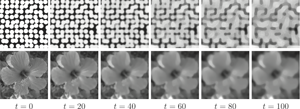
Fig. 9: Examples of gradient flows (39) at various times $t\stackrel{{\scriptstyle\mbox{\tiny def.}}}{{=}}k\tau$.

Figure 9 shows examples of gradient flows computed for the isotropic total variation $f(\mathrm{\textbf{a}})=|\!|\nabla\mathrm{\textbf{a}}|\!|_{1}$ as defined in (37). We use the discretization setup considered in Section 4.4, with the same value of $\varepsilon$, and a time-step $\tau=1/10$. This is exactly the regularization flow considered by [16], which is studied theoretically in [17]. This paper defines formally the highly nonlinear fourth order PDE corresponding to the limit flow. This is, however, not a “true” PDE since the initial TV functional is non-smooth, and derivatives should be understood in a weak sense, as limit of an implicit discrete time-stepping. While the algorithm proposed in [16] uses the usual (unregularized) Wasserstein distance, the use of a regularized transport allows us to deal with problems of larger sizes, with a faster numerical scheme. The price to pay is an additional blurring introduced by the entropic smoothing, but this is acceptable for applications to denoising in imaging. Figure 9 illustrates the behavior of this TV regularization flow, which has the tendency to group together clusters of mass and performs some kind of progressive “percolation” over the whole image.

Conclusion

In this paper, we introduced a dual framework for the resolution of certain variational problems involving Wasserstein distances. The key contribution is that the dual functional is smooth and that its gradient can be computed in closed form and involves only multiplications with a Gibbs kernel. We illustrate this approach with applications to several problems revolving around the idea of Wasserstein barycenters. This method is particularly advantageous for the computation of regularized barycenters, since precomposition by a linear operator (such as discrete gradient on images or graphs) of functionals is simple to handle. Our numerical finding is that entropic smoothing is crucial to stabilize the computation of barycenters and to obtain fast numerical schemes. Further regularization using, for instance, a total variation is also beneficial and can be used in the framework of gradient flows.

References

- Abraham et al. [2017] Isabelle Abraham, Romain Abraham, Maïtine Bergounioux, and Guillaume Carlier. Tomographic reconstruction from a few views: a multi-marginal optimal transport approach. Applied Mathematics & Optimization, 75(1):55–73, 2017.
- Agueh and Carlier [2011] M. Agueh and G. Carlier. Barycenters in the Wasserstein space. SIAM J. on Mathematical Analysis, 43(2):904–924, 2011.
- Allen-Zhu et al. [2017] Zeyuan Allen-Zhu, Yuanzhi Li, Rafael Oliveira, and Avi Wigderson. Much faster algorithms for matrix scaling. arXiv preprint arXiv:1704.02315, 2017.
- Ambrosio et al. [2006] L. Ambrosio, N. Gigli, and G. Savaré. Gradient flows in metric spaces and in the space of probability measures. Springer, 2006.
- Aurenhammer [1987] Franz Aurenhammer. Power diagrams: properties, algorithms and applications. SIAM Journal on Computing, 16(1):78–96, 1987.
- Aurenhammer et al. [1998] Franz Aurenhammer, Friedrich Hoffmann, and Boris Aronov. Minkowski-type theorems and least-squares clustering. Algorithmica, 20(1):61–76, 1998.
- Banerjee et al. [2005] A. Banerjee, S. Merugu, I. S Dhillon, and J. Ghosh. Clustering with Bregman divergences. The Journal of Machine Learning Research, 6:1705–1749, 2005.
- Bauschke and Combettes [2011] H. H. Bauschke and P. L. Combettes. Convex Analysis and Monotone Operator Theory in Hilbert Spaces. Springer-Verlag, New York, 2011.
- Beck and Teboulle [2009] A. Beck and M. Teboulle. A fast iterative shrinkage-thresholding algorithm for linear inverse problems. Journal on Imaging Sciences, 2(1):183–202, 2009.
- Benamou et al. [2015] J-D. Benamou, G. Carlier, M. Cuturi, L. Nenna, and G. Peyré. Iterative Bregman projections for regularized transportation problems. SIAM Journal on Scientific Computing, 37(2):A1111–A1138, 2015.
- Bigot and Klein [2012] J. Bigot and T. Klein. Consistent estimation of a population barycenter in the Wasserstein space. Preprint arXiv:1212.2562, 2012.
- Bonneel et al. [2011] N. Bonneel, M. van de Panne, S. Paris, and W. Heidrich. Displacement interpolation using lagrangian mass transport. ACM Transactions on Graphics (SIGGRAPH ASIA’11), 30(6), 2011.
- Bonneel et al. [2015] N. Bonneel, J. Rabin, G. Peyré, and H. Pfister. Sliced and radon Wasserstein barycenters of measures. Journal of Mathematical Imaging and Vision, 51(1):22–45, 2015.
- Bonneel et al. [2016] N. Bonneel, G. Peyré, and M. Cuturi. Wasserstein barycentric coordinates: Histogram regression using optimal transport. ACM Transactions on Graphics, 35(4), 2016.
- Boyd and Vandenberghe [2004] S. Boyd and L. Vandenberghe. Convex Optimization. Cambridge University Press, 2004.
- Burger et al. [2012] M. Burger, M. Franeka, and C-B. Schonlieb. Regularised regression and density estimation based on optimal transport. Appl. Math. Res. Express, 2:209–253, 2012.
- Carlier and Poon [2017] Guillaume Carlier and Clarice Poon. On the total variation wasserstein gradient flow and the tv-jko scheme. arXiv preprint arXiv:1703.00243, 2017.
- Carlier et al. [2015] Guillaume Carlier, Adam Oberman, and Edouard Oudet. Numerical methods for matching for teams and wasserstein barycenters. ESAIM: Mathematical Modelling and Numerical Analysis, 49(6):1621–1642, 2015.
- Caselles et al. [2007] V. Caselles, A. Chambolle, and M. Novaga. The discontinuity set of solutions of the TV denoising problem and some extensions. SIAM Multiscale Modeling and Simulation, 6(3):879–894, 2007.
- Cazelles et al. [2017] Elsa Cazelles, Jérémie Bigot, and Nicolas Papadakis. Regularized barycenters in the wasserstein space. In Frank Nielsen and Frédéric Barbaresco, editors, Geometric Science of Information, pages 83–90, Cham, 2017. Springer International Publishing.
- Chan [1996] Timothy M Chan. Optimal output-sensitive convex hull algorithms in two and three dimensions. Discrete & Computational Geometry, 16(4):361–368, 1996.
- Claici et al. [2018] Sebastian Claici, Edward Chien, and Justin Solomon. Stochastic Wasserstein barycenters. In ICML’18, 2018.
- Cohen et al. [2017] Michael B Cohen, Aleksander Madry, Dimitris Tsipras, and Adrian Vladu. Matrix scaling and balancing via box constrained newton’s method and interior point methods. In Foundations of Computer Science (FOCS), 2017 IEEE 58th Annual Symposium on, pages 902–913. IEEE, 2017.
- Cominetti and San Martín [1994] Roberto Cominetti and Jaime San Martín. Asymptotic analysis of the exponential penalty trajectory in linear programming. Mathematical Programming, 67(1-3):169–187, 1994.
- Courty et al. [2017] N. Courty, R. Flamary, D. Tuia, and A. Rakotomamonjy. Optimal transport for domain adaptation. IEEE Transactions on Pattern Analysis and Machine Intelligence, 39(9):1853–1865, Sept 2017. ISSN 0162-8828. 10.1109/TPAMI.2016.2615921.
- Cuturi [2013] M. Cuturi. Sinkhorn distances: Lightspeed computation of optimal transport. In Advances in Neural Information Processing Systems 26, pages 2292–2300, 2013.
- Cuturi and Doucet [2014] M. Cuturi and A. Doucet. Fast computation of Wasserstein barycenters. In Proceedings of the 31st International Conference on Machine Learning (ICML-14), pages 685–693, 2014.
- Cuturi and Peyré [2016] M. Cuturi and G. Peyré. A smoothed dual approach for variational wasserstein problems. SIAM Journal on Imaging Sciences, 9(1):320–343, 2016. 10.1137/15M1032600. URL http://arxiv.org/abs/1503.02533.
- De Goes et al. [2012] Fernando De Goes, Katherine Breeden, Victor Ostromoukhov, and Mathieu Desbrun. Blue noise through optimal transport. ACM Transactions on Graphics (TOG), 31(6):171, 2012.
- Franklin and Lorenz [1989] Joel Franklin and Jens Lorenz. On the scaling of multidimensional matrices. Linear Algebra and its applications, 114:717–735, 1989.
- Genevay et al. [2016] Aude Genevay, Marco Cuturi, Gabriel Peyré, and Francis Bach. Stochastic optimization for large-scale optimal transport. In Advances in Neural Information Processing Systems, pages 3440–3448, 2016.
- Gianazza et al. [2009] U. Gianazza, G. Savaré, and G. Toscani. The wasserstein gradient flow of the Fisher information and the quantum drift-diffusion equation. Archive for Rational Mechanics and Analysis, 194(1):133–220, 2009. ISSN 0003-9527. 10.1007/s00205-008-0186-5. URL http://dx.doi.org/10.1007/s00205-008-0186-5.
- Jordan et al. [1998] R. Jordan, D. Kinderlehrer, and O. Otto. The variational formulation of the Fokker-Planck equation. SIAM journal on mathematical analysis, 29(1):1–17, 1998.
- Knight and Ruiz [2013] Philip A Knight and Daniel Ruiz. A fast algorithm for matrix balancing. IMA Journal of Numerical Analysis, 33(3):1029–1047, 2013.
- Lee and Seung [1999] D. D. Lee and H. S. Seung. Learning the parts of objects by non-negative matrix factorization. Nature, 401(6755):788–791, 1999.
- Lellmann et al. [2014] Jan Lellmann, Dirk A Lorenz, Carola Schonlieb, and Tuomo Valkonen. Imaging with Kantorovich–Rubinstein discrepancy. SIAM Journal on Imaging Sciences, 7(4):2833–2859, 2014.
- Léonard [2014] Christian Léonard. A survey of the Schrödinger problem and some of its connections with optimal transport. Discrete and Continuous Dynamical Systems - A, 34:1533, 2014.
- Lévy [2015] Bruno Lévy. A numerical algorithm for semi-discrete optimal transport in 3d. ESAIM: Mathematical Modelling and Numerical Analysis, 49(6):1693–1715, 2015.
- Levy and Schwindt [2017] Bruno Levy and Erica Schwindt. Notions of optimal transport theory and how to implement them on a computer. arXiv:1710.02634, 2017.
- Maas et al. [2015] Jan Maas, Martin Rumpf, Carola Schönlieb, and Stefan Simon. A generalized model for optimal transport of images including dissipation and density modulation. ESAIM: Mathematical Modelling and Numerical Analysis, 49(6):1745–1769, 2015.
- Mérigot [2011] Q. Mérigot. A multiscale approach to optimal transport. Computer Graphics Forum, 30(5):1583–1592, 2011.
- Mérigot [2011] Quentin Mérigot. A multiscale approach to optimal transport. Comput. Graph. Forum, 30(5):1583–1592, 2011.
- Minsker et al. [2017] Stanislav Minsker, Sanvesh Srivastava, Lizhen Lin, and David B. Dunson. Robust and scalable bayes via a median of subset posterior measures. Journal of Machine Learning Research, 18(124):1–40, 2017. URL http://jmlr.org/papers/v18/16-655.html.
- Nielsen [2013] F. Nielsen. Jeffreys centroids: A closed-form expression for positive histograms and a guaranteed tight approximation for frequency histograms. IEEE Signal Processing Letters (SPL), 20(7), 2013.
- Oliker and Prussner [1989] Vladimir Oliker and Laird D Prussner. On the numerical solution of the equation and its discretizations, I. Numerische Mathematik, 54(3):271–293, 1989.
- Otto [2001] F. Otto. The geometry of dissipative evolution equations: the porous medium equation. Communications in partial differential equations, 26(1-2):101–174, 2001.
- Pele and Werman [2009] O. Pele and M. Werman. Fast and robust earth mover’s distances. In ICCV’09, 2009.
- Peyré and Cuturi [2018] G. Peyré and M. Cuturi. Computational optimal transport. Preprint 1803.00567, Arxiv, 2018. URL https://arxiv.org/abs/1803.00567.
- Peyré [2015] Gabriel Peyré. Entropic approximation of wasserstein gradient flows. SIAM Journal on Imaging Sciences, 8(4):2323–2351, 2015.
- Rabin and Papadakis [2015] J. Rabin and N. Papadakis. Convex color image segmentation with optimal transport distances. In Proc. SSVM’15, 2015.
- Rubner et al. [2000] Y. Rubner, C. Tomasi, and L.J. Guibas. The earth mover’s distance as a metric for image retrieval. IJCV: International Journal of Computer Vision, 40, 2000.
- Santambrogio [2015] Filippo Santambrogio. Optimal Transport for Applied Mathematicians. Birkhauser, 2015.
- Schmitzer [2016] B. Schmitzer. Stabilized sparse scaling algorithms for entropy regularized transport problems. arXiv:1610.06519, 2016.
- Schmitzer and Schnorr [2013] B. Schmitzer and C. Schnorr. Object segmentation by shape matching with wasserstein modes. In Proc. EMMCVPR’13, volume 8081 of Lecture Notes in Computer Science, pages 123–136. Springer Berlin Heidelberg, 2013.
- Sinkhorn [1964] Richard Sinkhorn. A relationship between arbitrary positive matrices and doubly stochastic matrices. Ann. Math. Statist., 35:876–879, 1964.
- Solomon et al. [2014] J. Solomon, R.M. Rustamov, L. Guibas, and A. Butscher. Wasserstein propagation for semi-supervised learning. In Proc. ICML 2014, 2014.
- Solomon et al. [2015a] J. Solomon, F. de Goes, G. Peyré, M. Cuturi, A. Butscher, A. Nguyen, T. Du, and L. Guibas. Convolutional wasserstein distances: Efficient optimal transportation on geometric domains. ACM Transactions on Graphics (Proc. SIGGRAPH 2015), to appear, 2015a. URL http://gpeyre.github.io/papers/2015-SIGGRAPH-convolutional-ot.pdf.
- Solomon et al. [2015b] Justin Solomon, Fernando De Goes, Gabriel Peyré, Marco Cuturi, Adrian Butscher, Andy Nguyen, Tao Du, and Leonidas Guibas. Convolutional Wasserstein distances: Efficient optimal transportation on geometric domains. ACM Transactions on Graphics (TOG), 34(4):66, 2015b.
- Sugiyama et al. [2017] Mahito Sugiyama, Hiroyuki Nakahara, and Koji Tsuda. Tensor balancing on statistical manifold. arXiv preprint arXiv:1702.08142, 2017.
- Swoboda and Schnorr [2013] P. Swoboda and C. Schnorr. Convex variational image restoration with histogram. SIAM J. Imag. Sci., 6(3):1719–1735, 2013.
- Villani [2009] C. Villani. Optimal transport: old and new, volume 338. Springer Verlag, 2009.
- Xia et al. [2014] G-S. Xia, S. Ferradans, G. Peyré, and J-F. Aujol. Synthesizing and mixing stationary gaussian texture models. SIAM Journal on Imaging Sciences, 7(1):476–508, 2014.
- Zen et al. [2014] G. Zen, E. Ricci, and N. Sebe. Simultaneous ground metric learning and matrix factorization with earth movers distance. Proc. ICPR’14, 2014.