Construction of an algebra corresponding to a statistical model of the square ladder (square lattice with two lines)

Abstract

In this paper we define infinite-dimensional algebra and its representation, whose basis is naturally identified with semi-infinite configurations of the square ladder model.

We also extrapolate the ideas for the cyclic 3-leg triangular ladder. All of these propose a way for generalization, which leads to representations of $N=2,\dots$ algebras.

Keywords: 2D lattice, square ladder, triangular ladder, conformal algebra, semi-infinite forms, fermions, quadratic algebra, superfrustration, graded Euler characteristic, cohomology, deformation, Jacobi triple product, superalgebras, operator algebras.

1 Introduction

For each graph $\Gamma$ we can construct a statistical model in which the set of configurations is the set of arrangements of particles at graph vertices such that at each vertex at most one particle is located and two particles cannot be located at vertices joined by an edge.

The previous paper $[1]$ discussed combinatorial properties of the set of configurations of the $2\times n$ square lattice (or simply the square ladder) graph:

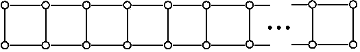
Figure 1: $2\times n$ square lattice model

Let’s assign the fermion algebra of anti-commuting elements $x_{i}$ and $y_{i}$ to the graph in Fig. 1, where $i=-k,\dots,k$ if $n=2k+1$ or $i=-k,\dots,k-1$ if $n=2k$; moreover, elements $x_{i},y_{i}$ satisfy the next relations:

$$x_{i}y_{i}=0,\;x_{i}x_{i+1}=0,\;y_{i}y_{i+1}=0.$$

Studies of integrable models of statistical mechanics show a close connection between the set of configurations of the corresponding lattice graph and the representation of some infinite-dimensional algebra $[2][3][4][5][6][7][8]$. Based on this, the paper yields the following results:

In Section 2, based on idea of semi-infinite forms, the set of configurations is defined for the square ladder model, which is infinite in both directions. A bigraduation is introduced and statistical sum is calculated.

In Section 3, such a deformation of the fermion algebra for the graph of the square ladder model, which is infinite in both directions, is determined (the obtained algebra is close to conformal algebras) that the character of its representation is equal to the statistical sum from Section 2.

In Section 4, the cohomology of complexes, constructed from finite-dimensional quotient algebras of the deformed algebra from Section 3, are calculated. The corresponding complexes are either acyclic, or their cohomology is one-dimensional. The deformation was selected by the latter, among other things.

In Section 5, further generalization is discussed.

2 Set of semi-infinite configurations

Instead of the square ladder model, Fig. 1, it is convenient to consider an equivalent combinatorial problem (the results of paper $[1]$ remain valid), the twisted square ladder model:

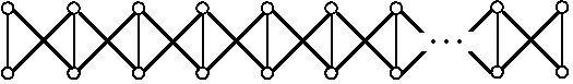
Figure 2: twisted square ladder model

According to $[8]$, the set $\Omega\subset\mathbb{Z}$ is called a Dirac set if $\Omega_{e}=\Omega\cap\mathbb{Z}_{\geq 0}$ and $\Omega_{p}=\mathbb{Z}_{<0}\setminus\Omega$ are finite. The value $C(\Omega)=\text{count}(\Omega_{e})-\text{count}(\Omega_{p})$ is called the charge of the set $\Omega$, and $U(\Omega)=\sum\limits_{\alpha\in\Omega_{e}\cup\Omega_{p}}|\alpha|$ is called its energy.

The set of such configurations $\{\dots,v_{i_{n-1}},v_{i_{n}},v_{i_{n+1}},\dots,v_{i_{1}}\}$ of the graph of the twisted square ladder model, which is infinite in both directions, that the set of indexes $\Omega=\{i_{n}\}$ is a Dirac set, is called the set of semi-infinite configurations $\Delta^{\frac{\infty}{2}}$. The location of particle $v_{i_{n}}$ is given by $x_{i_{n}}$ or $y_{i_{n}}$ depending on whether the particle is in the upper or lower row, where $i_{n}$ is the corresponding column number.

It follows from the definition of Dirac set that a configuration has “tail” (see Fig. 3), i.e. there is such $N\in\mathbb{Z}$ that

$$i_{N-j+1}=i_{N}-j+1\;\forall j\in\mathbb{N}.$$

Moreover, it follows from the definitions of set of configurations, Dirac set and the type of the graph under consideration (Fig. 2) that all $v_{i_{N-j+1}}$ are elements of one row.

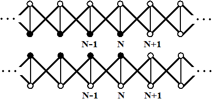
Figure 3: tails of twisted square ladder model

We will talk about energy and charge of $\{\dots,v_{i_{n-1}},v_{i_{n}},v_{i_{n+1}},\dots,v_{i_{1}}\}$ implying energy and charge of the corresponding set of indexes $\Omega=\{i_{n}\}$.

2.1 Calculation of statistical sum

In this subsection, our goal will be to calculate the statistical sum of the subset of configurations $\Delta^{\frac{\infty}{2}}$ with the fixed type of tail (Fig. 3) relative to $C$ and $U$, i.e.

$$F(t,q)=\sum_{across\;all\;Dirac\;sets\;\Omega}t^{C(\Omega)}q^{U(\Omega)}.$$

Proposition 1.

$$F(t,q)=\prod\limits_{m=1}^{\infty}\frac{1+q^{m}}{1-q^{m}}\sum\limits_{n=-\infty}^{\infty}q^{n(n-1)/2}t^{n}.$$

Proof. Let’s consider

$$F_{+}(t,q)=\sum_{\begin{subarray}{c}across\;all\;Dirac\;sets\;\Omega\\ with\;\Omega_{p}=\varnothing\end{subarray}}t^{C(\Omega)}q^{U(\Omega)}=\sum_{i=0}^{\infty}\varphi_{n}(q)t^{i}.$$

Lemma 1.

$$F_{+}(t,q)=\sum_{n=0}^{\infty}\frac{(q)^{+}_{n}}{(q)_{n}}q^{n(n-1)/2}t^{n},$$

where $(q)^{+}_{n}=(1+q)(1+q^{2})\dots(1+q^{n})$, $(q)_{n}=(1-q)(1-q^{2})\dots(1-q^{n})$.

Proof. One can readily see that the following is true

$$F_{+}(t,q)=tF_{+}(qt,q)+\dot{F}_{+}(qt,q),$$

where

$$\dot{F}_{+}(qt,q)=2tqF_{+}(q^{2}t,q)+\dot{F}_{+}(q^{2}t,q),$$

as we consider all possible options for particle arrangement at the column no. 0.

Then,

$$F_{+}(t,q)-tF_{+}(qt,q)=F_{+}(qt,q)-tqF_{+}(q^{2}t,q)+2tqF_{+}(q^{2}t,q).$$

Therefore, we obtain functional equation:

$$F_{+}(t,q)=F_{+}(qt,q)+t(F_{+}(qt,q)+qF_{+}(q^{2}t,q)).$$

Hence,

$$\varphi_{n}(q)=q^{n}\varphi_{n}(q)+q^{n-1}\varphi_{n-1}(q)+q^{2n-1}\varphi_{n-1}(q).$$

Consequently,

$$(1-q^{n})\varphi_{n}(q)=q^{n-1}(1+q^{n})\varphi_{n-1}(q).$$

As $\varphi_{0}(q)=1$, it has been demonstrated$._{\bigtriangledown}$

Let’s consider another statistical sum

$$F_{N}(t,q)=\sum_{\begin{subarray}{c}\text{across all Dirac sets $\Omega$:}\\ \text{$\Omega_{p}$ contains only the numbers not exceeding -N}\end{subarray}}t^{C(\Omega)}q^{U(\Omega)}.$$

Let’s consider the transformation associating the Dirac set $\Omega=\{i_{k}\}$ to the Dirac set $\Omega_{N}=\{i_{k}+N\}$. It is easily seen that $C(\Omega_{1})=C(\Omega)+1$ and $U(\Omega_{1})=U(\Omega)+C(\Omega)+1$. Following this, by induction,

$$C(\Omega_{N})=C(\Omega)+N\text{ and }U(\Omega_{N})=U(\Omega)+NC(\Omega)+N(N+1)/2.$$

A Dirac set contains all numbers not exceeding $-N$ if and only if $(\Omega_{N-1})_{p}=\varnothing$. This yields the equation

$$F_{+}(t,q)=t^{N-1}q^{N(N-1)/2}F_{N}(tq^{N-1},q).$$

Consequently,

$$F_{N}(t,q)=\frac{q^{(N-1)(N-2)/2}}{t^{N-1}}F_{+}(t/q^{N-1},q)=$$

$$=\sum_{n=0}^{\infty}\frac{(q)^{+}_{n}}{(q)_{n}}q^{n(n-1)/2+(N-1)(N-2)/2-n(N-1)}t^{n-N+1}=\sum_{n=-N+1}^{\infty}\frac{(q)^{+}_{n+N-1}}{(q)_{n+N-1}}q^{n(n-1)/2}t^{n}.$$

Going to the limit $N\longrightarrow\infty$, we obtain the required$._{\bigtriangledown}$

Remark.

$$\prod\limits_{m=1}^{\infty}\frac{1+q^{m}}{1-q^{m}}=\prod\limits_{m=1}^{\infty}\frac{1}{1-q^{m}}\prod\limits_{k=0}^{\infty}\frac{1}{1-q^{2k+1}}=$$

$$=(\prod\limits_{m=1}^{\infty}\frac{1}{1-q^{m}})^{2}\prod\limits_{k=1}^{\infty}(1-(q^{2})^{k}),$$

due to the equality of generating functions for splitting into odd and different summands $[9]$.

3 $\mathbf{SqL}$ algebra

The fermion algebra for the infinite in both directions graph as per Fig. 2 is the following algebra of anti-commuting elements $x_{i}$ and $y_{i}$, $i\in\mathbb{Z}$:

$$\mathbb{C}[\dots,x_{-1},y_{-1},x_{0},y_{0},x_{1},y_{1},\dots]/(x_{i}y_{i}=0,\;x_{i}y_{i+1}=0,\;x_{i+1}y_{i}=0).$$

Let’s determine the deformation of this algebra, namely the $\mathbf{SqL}$ algebra, generated by anti-commuting elements $x_{i}$, $y_{i}$, $i\in\mathbb{Z}$, satisfying the relations below (let’s denote it as $\verb"REL"$):

$$\forall s\in\mathbb{Z}\sum_{i\in\mathbb{Z}}x_{i}y_{-i+s}=0,\;\sum_{i\in\mathbb{Z}}x_{i}y_{-i+2s+1}(-1)^{i}=0,$$

with additional action of two operators $c$ and $u$:

$$[c,\;u]=0;\;$$

$$[c,\;x_{i}]=x_{i},\;[c,\;y_{i}]=y_{i};\;$$

$$[u,\;x_{i}]=-ix_{i},\;[u,\;y_{i}]=-iy_{i}.$$

Let’s denote generating functions $X(t)=\sum_{i\in\mathbb{Z}}x_{i}t^{-i}$, $Y(t)=\sum_{i\in\mathbb{Z}}y_{i}t^{-i}$, then the relations $\verb"REL"$ can be rewritten as

$$X(t)Y(t)=0,\;X(t)Y(-t)=X(-t)Y(t).$$

The relations $\verb"REL"$ are infinite; therefore, formally, the algebra with such relations has no sense. However, if we consider its representation in a graduated space, with peak limiting for the graduation, as is customary in the theory of conformal algebras, then everything will be determined.

Accordingly, for any integer $N$ let’s define induced representations with extreme vectors, i.e. spaces $\Upsilon(N)$ spawned by elements $x_{i},y_{i},$ $i\in\mathbb{Z}$, from the vectors $\gamma_{N}$, for which the following is true:

$$x_{i\geq N-1}\circ\gamma_{N}=0,\;y_{i\geq N}\circ\gamma_{N}=0.$$

In other words, $\Upsilon(N)=(\mathbb{C}[\dots,x_{-1},y_{-1},x_{0},y_{0},x_{1},y_{1},\dots]/\verb"REL")\circ\gamma_{N}$.

There are mappings

$$\dots\longrightarrow\Upsilon(-2)\longrightarrow\Upsilon(-1)\longrightarrow\Upsilon(0)\longrightarrow\Upsilon(1)\longrightarrow\dots,$$

which follow from $\gamma_{N-1}\longmapsto y_{N}\circ\gamma_{N}.$

Mappings $\Upsilon(N)\longrightarrow\Upsilon(N+1)$ are embeddings. This result is derived from the existence of monomial basis (Lemma 2) in $\Upsilon(N)$. Now we are going to discuss it. But, to begin with, let’s construct an auxiliary representation of the $\mathbf{SqL}$ algebra by using the Clifford algebra.

3.1 Constructing representation of $\mathbf{SqL}$ algebra

Let

$$\delta_{i+j}=\begin{cases}1,&i+j=0;\\ 0,&\text{otherwise.}\end{cases}$$

The algebra $OCl$ is generated by elements $o_{-2k-1},k\in\mathbb{N}\cup\{0\},$ $\varphi_{i},\varphi^{*}_{i},i\in\mathbb{Z}$, for which the following is true:

$$[o_{-2k-1},o_{-2l-1}]=0,[o_{-2k-1},\varphi_{i}]=0,[o_{-2k-1},\varphi^{*}_{i}]=0,$$

$$[\varphi_{i},\varphi_{j}]_{+}=0,[\varphi^{*}_{i},\varphi^{*}_{j}]_{+}=0,[\varphi_{i},\varphi^{*}_{j}]_{+}=\delta_{i+j}.$$

Moreover, additional action of $s$ and $w$ is defined:

$$[s,\;w]=0,\;$$

$$[s,\;\varphi_{i}]=\varphi_{i},\;[s,\;\varphi^{*}_{i}]=-\varphi^{*}_{i},\;[s,\;o_{-2i-1}]=0,$$

$$[w,\;\varphi_{i}]=-i\varphi_{i},\;[w,\;\varphi^{*}_{i}]=-i\varphi^{*}_{i},\;[w,\;o_{-2i-1}]=(2i+1)o_{-2i-1}.$$

Let’s introduce generating functions:

$$\varphi(z)=\sum\limits_{i\in\mathbb{Z}}\varphi_{i}z^{-i},o(z)=\sum\limits_{i\in\mathbb{N}\cup\{0\}}o_{-2i-1}z^{2i+1},\varphi^{*}(z)=\sum\limits_{i\in\mathbb{Z}}\varphi^{*}_{i}z^{-i}.$$

Let’s define:

$$\psi(z)=o(z)\varphi(z)=\sum\limits_{i\in\mathbb{Z}}\psi_{i}z^{-i},\text{ where }\psi_{i}=\sum\limits_{j+l=i}o_{j}\varphi_{l}.$$

The relations $\verb"REL"$ are fulfilled for $\varphi(z)$ and $\psi(z)$:

$$\varphi(z)\psi(z)=o(z)\varphi^{2}(z)=0,$$

$$\varphi(z)\psi(-z)=\varphi(z)\varphi(-z)o(-z)=-\varphi(z)\varphi(-z)o(z)=\varphi(-z)\psi(z).$$

Let’s suppose there exists extreme vector $v_{0}$:

$$\varphi_{i>0}\circ v_{0}=0,\varphi^{*}_{i\geq 0}\circ v_{0}=0.$$

Let’s set an action for $s$ and $w$ on $v_{0}$:

$$s\circ v_{0}=0,\;w\circ v_{0}=0.$$

The character of $OCl\circ v_{0}=\mathbb{C}[\varphi_{0},\varphi^{*}_{-1},o_{-1},\varphi_{-1},\dots]\circ v_{0}$ is defined as $Tr_{OCl\circ v_{0}}(q^{w}t^{s}).$

Proposition 2.

$Tr_{OCl\circ v_{0}}(q^{w}t^{s})$ and $F(t,q)$ coincide.

Proof. As is well known, the character of the space of polynomials in anti-commuting variables $\varphi_{i},\varphi^{*}_{i-1},i=0,-1,\dots,$ is equal to

$$\prod\limits_{j=0}^{\infty}(1+q^{j}t)\prod\limits_{k=1}^{\infty}(1+q^{k}t^{-1}),$$

which equals to

$$(\prod\limits_{l=1}^{\infty}\frac{1}{1-q^{l}})\sum\limits_{n=-\infty}^{\infty}q^{n(n-1)/2}t^{n}$$

according to the Jacobi triple product $[9]$.

Moreover, as is well known, the character of the space of polynomials in commuting variables $o_{2i-1},i=0,-1,\dots,$ is equal to

$$\prod\limits_{m=0}^{\infty}\frac{1}{1-q^{2m+1}}._{\bigtriangledown}$$

3.2 Direct limit

Lemma 2.

In $\Upsilon(N)$ there is a monomial basis consisting of

$$x_{i_{1}}x_{i_{2}}\dots x_{i_{l}}y_{j_{1}}y_{j_{2}}\dots y_{j_{m}}\circ\gamma_{N},|i_{a}-j_{b}|\geq 2.$$

Proof. Using $\verb"REL"$, as well as skew symmetry, any monomial $x_{\widetilde{z}_{1}}\dots x_{\widetilde{z}_{k}}y_{\widetilde{t}_{1}}\dots y_{\widetilde{t}_{l}}$ can be expressed in the required form as above (see $[7]$ and $[8]$): each of newly appeared monomials will be lexicographically less than the original ($\text{deg}(x_{j})=\text{deg}(y_{j})=j$, all $y_{j}$ follow after all $x_{i}$). Of course, newly appeared monomials may contain pairs breaking the conditions $|i_{a}-j_{b}|\geq 2$, but the lexicographical order allows to develop an iterative procedure.

Let’s demonstrate the linear independence. For this purpose, let’s use $\mathbf{SqL}$ representation defined above. Let’s set the homomorphism of algebras:

$$x_{i}\longmapsto\varphi_{i},\;y_{i}\longmapsto\psi_{i},\;u\longmapsto w,\;c\longmapsto s,$$

from here we obtain the mapping of spaces:

$$\Upsilon(N)\longrightarrow\Upsilon_{\varphi,\psi}(N)=\mathbb{C}[\dots,\varphi_{-1},\psi_{-1},\varphi_{0},\psi_{0},\varphi_{1},\psi_{1},\dots]\circ\gamma_{N}.$$

By definition, $\psi_{i}=\sum\limits_{j+l=i}o_{j}\varphi_{l}$ acts with non-zero to $\gamma_{N}$ only with a finite number of $o_{j}\varphi_{l},$ therefore:

$$\Upsilon_{\varphi,\psi}(N)=\mathbb{C}[\dots,\varphi_{-2},o_{-2},\varphi_{-1},o_{-1},\varphi_{0},\varphi_{1},\varphi_{2},\dots]\circ\gamma_{N}.$$

By definition of $\gamma_{N}$, the latter is

$$\mathbb{C}[\dots,\varphi_{-2},o_{-2},\varphi_{-1},o_{-1},\varphi_{0}][\varphi_{1},\varphi_{2},\dots,\varphi_{N-1}]\circ\gamma_{N}.$$

Then, from the definition of $OCl$, we obtain the following isomorphism:

$$\Upsilon_{\varphi,\psi}(N)\simeq\begin{cases}\mathbb{C}[\varphi_{0},o_{-1},\varphi_{-1},o_{-3},\dots][\varphi^{*}_{-1},\varphi^{*}_{-2},\dots,\varphi^{*}_{-N+1}]\circ v_{0},&\text{$N>0$,}\\ \mathbb{C}[\varphi_{0},o_{-1},\varphi_{-1},o_{-3},\dots]\circ\varphi_{N}\dots\varphi_{0}\circ v_{0},&\text{$N\leq 0$.}\end{cases}$$

Therefore,

$$OCl\circ v_{0}=\mathbb{C}[\varphi_{0},\varphi^{*}_{-1},o_{-1},\varphi_{-1},\dots]\circ v_{0}=\varinjlim\Upsilon_{\varphi,\psi}(N).$$

Thereafter, there are no additional relationships for $x_{i_{1}}x_{i_{2}}\dots x_{i_{l}}y_{j_{1}}y_{j_{2}}\dots y_{j_{m}}\circ\gamma_{N},$ where $|i_{a}-j_{b}|\geq 2$, because otherwise the character $Tr_{OCl\circ v_{0}}(q^{w}t^{s})$ would be less than the statistical sum $F(t,q)$, but from Proposition 2 we know that this is not so._▽

Let’s define

$$\Upsilon=\varinjlim\Upsilon(N).$$

Any vector of space $\Upsilon$ is a finite linear combination of expressions

$$x_{i_{1}}x_{i_{2}}\dots x_{i_{l}}y_{j_{1}}y_{j_{2}}\dots y_{j_{m}}\circ\gamma_{N}=x_{i_{1}}x_{i_{2}}\dots x_{i_{l}}y_{j_{1}}y_{j_{2}}\dots y_{j_{m}}y_{N}\circ\gamma_{N+1}=\dots,$$

$$|i_{a}-j_{b}|\geq 2,$$

for a sufficiently large $N$. Let’s send $N$ to infinity, i.e. formally substitute $\gamma_{N}$ with expression

$$y_{N}y_{N+1}y_{N+2}\dots\circ\gamma_{\infty}.$$

So, we obtain the representation, which can be naturally identified with the set of semi-infinite configurations with the fixed type of tail.

Let’s set an action of $c$ and $u$ on extreme vectors $\gamma_{N}$:

$$c\circ\gamma_{N}=-N\gamma_{N},$$

$$u\circ\gamma_{N}=\begin{cases}\frac{N(N+1)}{2}\gamma_{N},&\text{$N\geq 0$,}\\ \frac{N(N-1)}{2}\gamma_{N},&\text{$N<0$.}\end{cases}$$

The character of $\Upsilon$ is defined as $Tr_{\Upsilon}(q^{u}t^{c}).$

Proposition 3.

$Tr_{\Upsilon}(q^{u}t^{c})$ and $F(t,q)$ coincide.

Proof. After all the above it’s obvious._▽

4 Cohomology

Let’s define algebra $A_{n}$ of anti-commuting elements $x_{i}$ and $y_{i}$, where $i=-k,\dots,k$ if $n=2k+1$ or $i=-k,\dots,k-1$ if $n=2k$, satisfying the relations $\verb"REL"$ (all other $x_{j}$ and $y_{j}$, with other indexes, are assumed equal to zero).

Therefore, algebra $A_{n}$ is a finite-dimensional quotient algebra of $\mathbf{SqL}$. It follows from Lemma 2 that the dimension of $A_{n}$ is identical to the dimension of the fermion algebra of the twisted square ladder with $n$ columns. Moreover, they have the same monomial basis.

Symbols $x_{i}$ or $y_{i}$ also denote the operator of multiplication by the corresponding element.

Let’s construct a complex $K_{n}\cong A_{n}$ with differential $x_{0}+y_{0}$.

Let’s introduce elements from $K_{2k+1}$, which are defined recursively as follows:

$$\underline{h}_{2k+1}=\begin{cases}x_{-k}\underline{h}_{2k-3}y_{k},&\text{$k\mod 2\neq 0$,}\\ y_{-k}\underline{h}_{2k-3}y_{k},&\text{$k\mod 2=0$,}\end{cases}$$

$$\overline{h}_{2k+1}=\begin{cases}y_{-k}\underline{h}_{2k-3}x_{k},&\text{$k\mod 2\neq 0$,}\\ x_{-k}\underline{h}_{2k-3}x_{k},&\text{$k\mod 2=0$,}\end{cases}$$

where $\underline{h}_{3}=x_{-1}y_{1},\overline{h}_{3}=y_{-1}x_{1};$ $\underline{h}_{1}=y_{0},\overline{h}_{1}=y_{0},$ $k\in\mathbb{N}\bigcup\{0\}$.

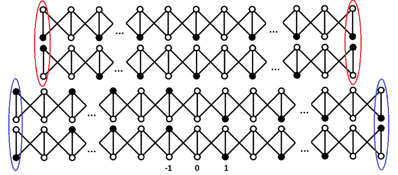
Figure 4: $\underline{h}_{2k+1}$ and $\overline{h}_{2k+1}$

Proposition 4.

The cohomology of the complexes $K_{2k+1},\;K_{2k+2}$ is one-dimensional. The element $\underline{h}_{2k+1}$ is a representative of the corresponding cohomoloogy class in both cases.

Proof. To begin with, let’s consider the odd case, $K_{2k+1}$.

Note that if $2s=\pm 2k$, from $\sum_{i\in\mathbb{Z}}x_{i}y_{-i+2s}=0$ it follows that

$$x_{-k}y_{-k}=0=x_{k}y_{k}.$$

In addition, if $2s+1=-2k+1,2k-1$, it follows from $\sum_{i\in\mathbb{Z}}x_{i}y_{-i+2s+1}=0$ and $\sum_{i\in\mathbb{Z}}x_{i}y_{-i+2s+1}(-1)^{i}=0$ that

$$x_{-k}y_{-k+1}=x_{-k+1}y_{-k}=0,\;x_{k}y_{k-1}=x_{k-1}y_{k}=0.$$

Then, let’s introduce auxiliary complexes denoted as $K^{\alpha,\beta}_{2k+1},\alpha,\beta\in\{x,y,\square\}.$

$K^{x,x}_{2k+1}$ means the image of operator of multiplication by $x_{-k}x_{k}:$ $x_{-k}x_{k}K_{2k+1},$ $K^{x,y}_{2k+1}$ means the image of $x_{-k}y_{k}:$ $x_{-k}y_{k}K_{2k+1}.$ $K^{x,\square}_{2k+1}$ means the factor space of the image of operator of multiplication by $x_{-k}:$ $x_{-k}K_{2k+1}/\{x_{k}=0,\;y_{k}=0\},$ $K^{\square,x}_{2k+1}$ is $x_{k}K_{2k+1}/\{x_{-k}=0,\;y_{-k}=0\}.$

Similar for $K^{y,y}_{2k+1}$, $K^{y,x}_{2k+1}$, $K^{y,\square}_{2k+1}$, $K^{\square,y}_{2k+1}$.

$K^{\square,\square}_{2k+1}$ means $K_{2k+1}/\{x_{-k}=0=y_{-k},\;x_{k}=0=y_{k}\}=K_{2k-1}.$

Therefore, we split $K_{2k+1}$, see Lemma 2 and $[1]$.

Lemma 3.

The complexes $K^{x,\square}_{2k+1},K^{y,\square}_{2k+1},K^{\square,x}_{2k+1},K^{\square,y}_{2k+1}$ are acyclic.

The cohomology of the complexes $\text{K}^{x,x}_{2k+1}$, $\text{K}^{y,y}_{2k+1}$ is one-dimensional in case of odd $k$, and elements $\overline{h}_{2k+1}$, $\underline{h}_{2k+1}$ are a representatives of the corresponding cohomology class, respectively. If $k$ is even, then the complexes are acyclic.

The cohomology of the complexes $\text{K}^{x,y}_{2k+1}$, $\text{K}^{y,x}_{2k+1}$ is one-dimensional in case of even $k$, and elements $\underline{h}_{2k+1}$, $\overline{h}_{2k+1}$ are a representatives of the corresponding cohomology class, respectively. If $k$ is odd, then the complexes are acyclic.

We prove Lemma 3 and Proposition 4 for the odd case by induction.

The reader is encouraged to check the induction base for $K^{\alpha,\beta}_{2k+1}$, $k\leq 3$, $K_{m}$, $m\leq 3$.

Applying simultaneous induction, we use the following considerations.

There exist an exact triple (because of the monomial basis, see Lemma 2):

$$0\longrightarrow\bigoplus\limits_{\alpha\neq\square\text{ and }\beta\neq\square}K^{\alpha,\beta}_{2k+3}\longrightarrow K_{2k+3}\longrightarrow\bigoplus\limits_{\alpha=\square\text{ or }\beta=\square}K^{\alpha,\beta}_{2k+3}\longrightarrow 0$$

As is well known, a long exact sequence of cohomologies is associated with exact triple. But due to the inductive assumption, we obtain the next exact sequence for $K_{2k+3}$:

$$0\longrightarrow H^{k+1}(K_{2k+3})\longrightarrow H^{k+1}(K_{2k+1})\longrightarrow H^{k+2}(\bigoplus\limits_{\alpha\neq\square\text{ and }\beta\neq\square}K^{\alpha,\beta}_{2k+3})\longrightarrow H^{k+2}(K_{2k+3})\longrightarrow 0$$

Similar exact sequences can also be written for all $K^{\alpha,\beta}_{2k+3}.$

Because we know Euler characteristics of all $K^{\alpha,\beta}_{2l+1}$ and $K_{2l+1}$ itself for any $l$ (absolute values do not exceed 1) from paper $[1]$ and thanks to Lemma 2, then, to prove the simultaneous induction, we just need to show that

$$(x_{0}+y_{0})\circ\underline{h}_{2k+1}\neq 0$$

in corresponding “2k+3” spaces.

Up to a change of basis, we have:

$$(x_{0}+y_{0})\underline{h}_{2k+1}=\begin{cases}(x_{0}+y_{0})x_{-k}\underline{h}_{2k-3}y_{k}=x_{-k}\underline{h}_{2k-1}y_{k},&\text{$k\mod 2\neq 0$,}\\ (x_{0}+y_{0})y_{-k}\underline{h}_{2k-3}y_{k}=y_{-k}\underline{h}_{2k-1}y_{k},&\text{$k\mod 2=0$.}\end{cases}$$

An element $x_{-k}\underline{h}_{2k-1}y_{k}\;(y_{-k}\underline{h}_{2k-1}y_{k})$ contains only one “prohibited” pair:

$$x_{-k}y_{-k+1}\;(y_{-k}x_{-k+1})$$

It follows from the relations $\verb"REL"$ in $K_{2k+3}$ that

$$x_{-k}y_{-k+1}=-x_{-k+2}y_{-k-1},\;$$

$$y_{-k}x_{-k+1}=-y_{-k+2}x_{-k-1}.$$

Using the latter equations, it is possible to rewrite $x_{-k}\underline{h}_{2k-1}y_{k}\;(y_{-k}\underline{h}_{2k-1}y_{k})$ as an element of the monomial basis, therefore, it is not equal to zero, see Lemma 2.

The statement for $K_{2k}$ follows from the statement for $K_{2k-1}$ and Lemma 3, as it is possible to write exact triple for $K_{2k}$ with $K_{2k-1}$ and $K^{x,\square}_{2k-1},K^{y,\square}_{2k-1}._{\bigtriangledown}$

Example.

$(x_{0}+y_{0})(x_{-1}y_{1}+x_{1}y_{-1})\neq 0\text{ in }K_{5}$

Let’s use the relation $x_{-2}y_{2}+x_{2}y_{-2}+x_{0}y_{0}=-(x_{-1}y_{1}+x_{1}y_{-1}):$

$$-(x_{0}+y_{0})(x_{-1}y_{1}+x_{1}y_{-1})=(x_{0}+y_{0})(x_{-2}y_{2}+x_{2}y_{-2})\neq 0.$$

5 Appendix: a generalization

Conjecture is that it is possible to universalize the ideas for some m-leg ladder models. That way, we obtain representations of $N=2,\dots$ algebras.

5.1 Graded Euler characteristic

Let’s recall basic definitions.

For each graph $\Gamma$ we can construct a statistical model in which the set of configurations is the set of arrangements of particles at graph vertices such that at each vertex at most one particle is located and two particles cannot be located at vertices joined by an edge.

To any graph $\Gamma$ there corresponds the fermion algebra $A(\Gamma)$ defined as follows.

Let $S$ be the vertex set of $\Gamma$, and let $T\subset S\times S$ be its edge set. The algebra $A(\Gamma)$ is generated by $\psi_{s},s\in S$. The defining relations are

$$\psi_{s_{1}}\psi_{s_{2}}+\psi_{s_{2}}\psi_{s_{1}}=0,\;\psi_{s_{1}}\psi_{s_{2}}=0,(s_{1},s_{2})\in T.$$

From $A(\Gamma)$ we can construct a complex $K(\Gamma)\cong A(\Gamma)$ with differential $\sum\limits_{s\in S}\psi_{s}$.

The statistical sum of the model is the sum over the space of all configurations. The contribution of each configuration depends on parameters. For some parameters values, the contribution of any configuration to the statistical sum equals $\pm 1$, depending on the parity of the number of particles in the given configuration. This statistical sum is naturally interpreted as the Euler characteristic of the complex $K(\Gamma)$.

By a weight system $\{w\}$ on the graph $\Gamma$ we mean a function on $S$ assigning a number $w(s)$ to each vertex $s$. For each configuration $\chi=\{s_{1},s_{2},\dots,s_{l}\}$ we define its energy

$$E^{w}(\chi)=(-1)^{l}q^{\sum\limits_{i=1}^{l}w(s_{i})},q\in\mathbb{C}^{*}.$$

We introduce the statistical sum $\sum E^{w}(\chi)$, where the summation is over all configurations. We refer to this as the graded Euler characteristic and denote it by $\text{E}_{q}^{\text{w}}(\Gamma)$.

5.2 Cyclic 3-leg triangular ladder model

Cyclic 3-leg triangular ladder is the 4-leg triangular ladder, where first and last rows coincide (are glued), see Fig. 5.

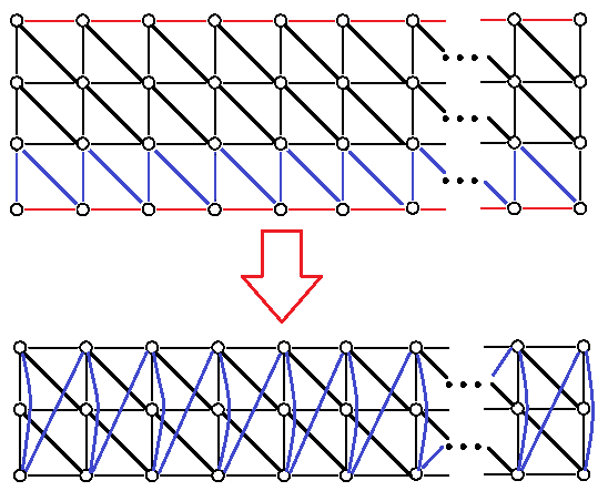
Figure 5: cyclic 3-leg triangular ladder with $n$ columns

We denote the graph from Fig. 5 by $\Gamma^{3}_{n}$.

Let $E^{3}_{n}$ denote the Euler characteristic of the complex $K(\Gamma^{3}_{n})$.

Proposition 5.

$E^{3}_{n}=(E^{3}_{1})^{[\frac{n+1}{2}]}=(-2)^{[\frac{n+1}{2}]}$, where $[*]$ denotes the integer part of a number.

Proof. It is easy to see that such relation holds:

$$E^{3}_{n}=E^{3}_{1}E^{3}_{n-2},$$

as any non-empty arrangement of particles in second column of Fig. 5 partitions the graph into two disconnected graphs, one of which is a one-point space. The Euler characteristic of a disconnected graph is the product of the Euler characteristics of its connected components.

In addition, $E^{3}_{1}=-2._{\bigtriangledown}$

Let’s consider the weight system (which we denote by $f$), where each fermion in the column number $i$, $i=1,\dots,n,$ has weight $[\frac{n}{2}]+i-1$.

To the cyclic 3-leg triangular ladder with $n$ columns we assign a table of weights and numbers of fermions; namely, each cell of this table contains the number of all admissible arrangements of a given number of fermions with given weights.

The number of a column in the table corresponds to the number of arranged fermions. The first column corresponds to $0$ fermions; it is impossible to arrange more than $n$ fermions. The rows correspond to weights. We assume that the configuration with no fermions has weight $0$.

Below we give examples of such tables. We leave a cell empty if there exist no configurations with given weight and given number of fermions.

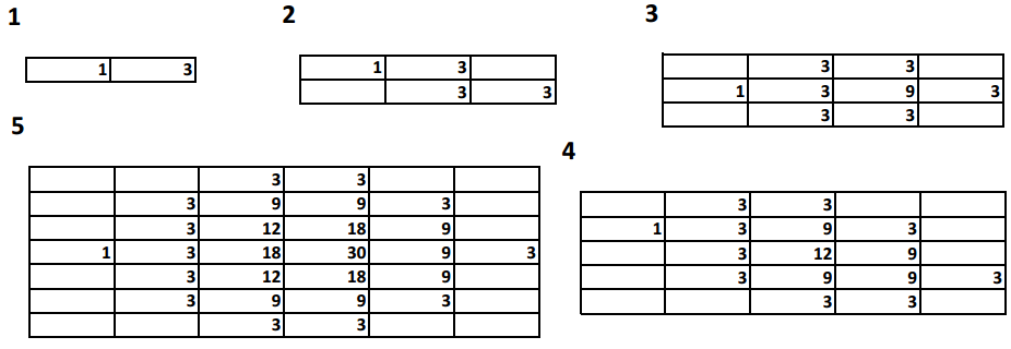
Figure 6: first tables

For each $j=0,\dots,n,$ to the $j$th column of a table there naturally corresponds a Laurent polynomial in the independent variable $q$. We denote these polynomials by $g^{j}_{n}(q)$. For example, $g^{3}_{3}(q)=3q+9+3q^{-1}$.

Clearly, $\text{E}^{f}_{q}(\Gamma^{3}_{n})=\sum\limits_{i=0}^{n}(-1)^{i}g_{n}^{j}(q).$

Proposition 6.

The relation $\text{E}^{f}_{q}(\Gamma^{3}_{n})=E^{3}_{n}$ holds.

Proof. This can be proved in the same manner as in paper $[1]._{\bigtriangledown}$

All definition connected with semi-infinite configurations are the same. The reader is encouraged to check it.

Proposition 7.

$$\widehat{F}(t,q)=\prod\limits_{m=1}^{\infty}\frac{1+2q^{m}}{1-q^{m}}\sum\limits_{n=-\infty}^{\infty}q^{n(n-1)/2}t^{n},$$

where $\widehat{F}(t,q)$ means the statistical sum of the set of semi-infinite configurations in case of the cyclic 3-leg triangular ladder with the fixed type of tail relative to $C$ and $U._{\bigtriangledown}$

The fermion algebra for the infinite in both directions graph as per Fig. 5 is the following algebra of anti-commuting elements $x_{i}$, $y_{i}$ and $z_{i}$, $i\in\mathbb{Z}$:

$$\mathbb{C}[\dots,x_{-1},y_{-1},z_{-1},x_{0},y_{0},z_{0},x_{1},y_{1},z_{1},\dots]$$

with relations:

$$x_{i}y_{i}=0,\;x_{i}y_{i+1}=0;$$

$$y_{i}z_{i}=0,\;y_{i}z_{i+1}=0;$$

$$z_{i}x_{i}=0,\;z_{i}x_{i+1}=0;$$

$$x_{i}x_{i+1}=0,\;y_{i}y_{i+1}=0,\;z_{i}z_{i+1}=0.$$

Let’s denote generating functions

$$X(t)=\sum_{i\in\mathbb{Z}}x_{i}t^{-i},\;Y(t)=\sum_{i\in\mathbb{Z}}y_{i}t^{-i},\;Z(t)=\sum_{i\in\mathbb{Z}}Z_{i}t^{-i}.$$

Let’s determine the deformation of the fermion algebra for the infinite in both directions graph as per Fig. 5. It is the algebra, generated by anti-commuting elements $x_{i}$, $y_{i}$ and $z_{i}$, satisfying relations below:

$$X(t)Y(t)=0,\;Y(t)Z(t)=0,\;Z(t)X(t)=0,$$

$$X(t)X(-t)=0,\;Y(t)Y(-t)=0,\;Z(t)Z(-t)=0.$$

The deformation preserves dimensions in the corresponding induced representations with extreme vectors.

5.3 Another model

Let’s consider such graph (which we denote by $\widetilde{\Gamma}^{m}_{n}$):

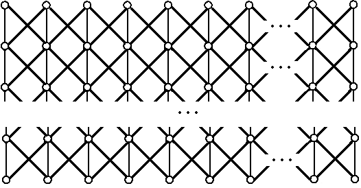
Figure 7: m-leg ladder with $n$ columns

Let $\widetilde{E}^{m}_{n}$ denote the Euler characteristic of the complex $K(\widetilde{\Gamma}^{m}_{n})$.

Proposition 8.

$\widetilde{E}^{m}_{n}=(\widetilde{E}^{m}_{1})^{[\frac{n+1}{2}]}$, where $[*]$ denotes the integer part of a number.

Proof. It is easy to see that such relation holds:

$$\widetilde{E}^{m}_{n}=\widetilde{E}^{m}_{1}\widetilde{E}^{m}_{n-2},$$

by the same reasons as in Proposition 5.

Moreover,

$$\widetilde{E}^{m}_{1}=-\widetilde{E}^{m-3}_{1},$$

where

$$\widetilde{E}^{1}_{1}=0,\;\widetilde{E}^{2}_{1}=-1,\;\widetilde{E}^{3}_{1}=-1._{\bigtriangledown}$$

Let’s recall the weight system (which is denoted by $f$), where each fermion in the column number $i$, $i=1,\dots,n,$ has weight $[\frac{n}{2}]+i-1$.

Proposition 9.

$E^{f}_{q}(\widetilde{\Gamma}^{3}_{1})=\widetilde{E}^{3}_{1},$ $E^{f}_{q}(\widetilde{\Gamma}^{3}_{2})=\widetilde{E}^{3}_{2},$ $E^{f}_{q}(\widetilde{\Gamma}^{3}_{3})=3-q-q^{-1}\neq\widetilde{E}^{3}_{3}.$

Proof. A direct calculation$._{\bigtriangledown}$

Remark.

Proposition 9 does not mean that the idea does not work due to Proposition 5.

Let $\Theta$ denote such set of weight systems, for which is assumed that each fermion in the column number $1$ on Fig. 7 has weight $0$.

Proposition 10.

The relation $E^{\text{o}}_{q}(\widetilde{\Gamma}^{3m+1}_{n})=\widetilde{E}^{3m+1}_{n}$ holds for any $o\in\Theta.$

Proof. It follows from Proposition 8, as $\widetilde{E}^{3m+1}_{1}=0._{\bigtriangledown}$

Higher School of Economics – National Research University, Moscow
VvS@myself.com

References

[1] Feigin B.L., Sopin V.V., Combinatorics of a Statistical Model Constructed from the Square Lattice, Funkt. Anal. i Prilozhen., V. 51, N. 4, 2017, 72 – 78.
[2] Lepowsky J., Primc M., Structure of the standard modules for the affine Lie algebra , Contemp. Math., V. 46, 1985, 1 – 84.
[3] Bouwknegt P., Ludwig A., Schoutens K., Spinon basis for integrable highest weight modules and new character formula, Proc. of Statistical Mechanics and Quantum Field theor, 1994, 16 – 21.
[4] Foda O., Miwa T., Corner transfer matrices and quantum affine algebras, Preprint hep-th/9204068, 1992.
[5] Kashiwara M., Miwa T., Petersen J., Yung C., Perfect crystals and q-deformed Fock spaces, Selecta Mathematica, V. 3, N. 3, 1996, 415 – 499.
[6] Semikhatov A.M., Tipunin I.Yu., Feigin B.L., Semi-Infinite Realization of Unitary Representations of the Algebra and Related Constructions, Teoret. Mat. Fiz., V. 126, V. 1, 2001, 3 – 62.
[7] Stoyanovskii A.V., Feigin B.L., Functional Models for Representations of Current Algebras and Semi-Infinite Schubert Cells, Funktsional. Anal. i Prilozhen., V. 28, N. 1, 1994, 68 – 90.