Thermodynamic Behaviour of Magnetized QGP within the Self-Consistent Quasiparticle Model

Abstract

The self-consistent quasiparticle model has been successful in studying QCD thermodynamics. In this model, the medium effects are taken into account by considering quarks and gluons as quasiparticles with temperature dependent masses which are proportional to the plasma frequency. The present work involves the extension of this model in the presence of magnetic fields. We have included the effect of the magnetic field by considering relativistic Landau Levels. The quasiparticle masses are then found to be dependent on both temperature and magnetic field. The thermo-magnetic mass thus defined allows obtaining the thermodynamics of magnetised quark matter within the self-consistent quasiparticle model. The model then has been applied to the case of 2-flavor Quark-Gluon Plasma and the equation of state obtained in the presence of magnetic fields.

I Introduction

High energy collisions have succeeded in recreating the state of matter called Quark Gluon Plasma (QGP) which is believed to have existed shortly after the big bang. It has been observed that QGP produced in high energy collisions behave very much like a nearly perfect fluid Back et al. (2005); *adams1; *adcox1; *arsene1. These collisions mostly occur with a finite impact parameter. During off central collisions, the charged ions thus can produce very large magnetic fields reaching up to $eB\approx(1-5)m_{\pi}^{2}$ SKOKOV et al. (2009); Yang et al. (2015). These magnetic fields may exist only for a short time but, depending on the transport coefficients, they may reach their maximum value and can be stationary during this time Tuchin (2011); Marasinghe and Tuchin (2011); Tuchin (2010); Fukushima and Pawlowski (2012). The magnetic field can cause different phenomena like magnetic catalysis Gusynin et al. (1994); cat (2013); Gusynin et al. (1996); Fukushima and Hidaka (2013), chiral magnetic effect Fukushima et al. (2008); Kharzeev et al. (2008); Kharzeev (2014), etc. in the QGP. The equation of state is important for studying the particle spectra created in heavy-ion collisions. Very strong magnetic fields are estimated to have existed right after the big bang Grasso and Rubinstein (2001). Effects of external magnetic fields are relevant in the context of strongly magnetised neutron stars too Duncan and Thompson (1992); *Broderick2000; *Cardall2001; *Rabhi2008; *Rabhi2011. Therefore, it is of importance to investigate the behaviour of QGP under magnetic fields, in particular, the effect on the QCD thermodynamics Strickland et al. (2012); Avancini et al. (2018). There have been several investigations as to how these magnetic fields affect the transport coefficients Kurian and Chandra (2018); Kurian et al. .

In this work, we intend to understand the effect of magnetic fields on QCD thermodynamics and obtain the equation of state by extending a quasiparticle model for QGP, called the self-consistent quasiparticle model. We incorporate the effect of the magnetic field by modifying the thermal mass using the relativistic Landau Levels. Such modified masses in the presence of magnetic fields can be used to calculate thermodynamic quantities like energy density, pressure, entropy density, etc. Besides, by applying this formalism to the 2-flavor system, we obtain its thermodynamics in the presence of background magnetic field and examine the qualitative behaviour of the equation of state.

II The self-consistent quasiparticle model

In quasiparticle models, the thermal properties of interacting real particles are modelled by noninteracting quasiparticles. The quasiparticles have an effective mass which is determined by the collective properties of the medium Goloviznin and Satz (1993); Peshier et al. (1994). Such models include the Nambu-Jona-Lasinio and PNJL based quasiparticle models Dumitru and Pisarski (2002); *Fukushima2004; *Ghosh2006; *Abuki2009; *Tsai2009 or those that include effective mass with the Polyakov loop D’Elia et al. (1997); *Castorina2007; *Castorina2007a. There are also quasiparticle models based on Gribov-Zwanziger quantisation Su and Tywoniuk (2015). Other effective mass quasiparticle models include self-consistent and single parameter quasiparticle models Bannur (2007a, b, c, d, 2008). There are quasiparticle models which incorporate the medium effects by considering quasiparticles with effective fugacities too. Such models have been quite successful in describing the lattice QCD results Chandra and Ravishankar (2009, 2011).

The self-consistent quasiparticle model here considers QGP as consisting of non-interacting quasiparticles with effective masses which depend on thermodynamic quantities and encode all medium interactions Bannur (2007a, 2008). Since the thermal mass depends on thermodynamic quantities which in turn depends on thermal mass, the whole problem is solved self-consistently.

In the self-consistent model, following standard thermodynamics, all thermodynamic quantities are derived from the expressions for energy density and number density. The expression for energy density is,

$$\varepsilon=\frac{g_{f}}{2\pi^{2}}\int_{0}^{\infty}dk\;k^{2}\frac{\omega_{k}}{z^{-1}e^{\frac{\omega_{k}}{T}}\mp 1},$$ (1)

where $g_{f}$ is the degeneracy and $\mp$ refers to bosons and fermions. $z$ is the fugacity. The expression for number density is,

$$n_{g/q}=\frac{g_{f}}{2\pi^{2}}\int_{0}^{\infty}dk\;k^{2}\frac{1}{z^{-1}e^{\frac{\omega_{k}}{T}}\mp 1}.$$ (2)

The single particle energy $\omega_{k}$ is approximated to a simple form,

$$\omega_{k}=\sqrt{k^{2}+m_{g}^{2}}$$ (3)

and

$$\omega_{k}=\sqrt{k^{2}+m_{q}^{2}},$$ (4)

for gluons and quarks respectively. This approximation is valid at high temperatures only.

It is known that quasiparticles acquire ”thermal mass” of order $gT$ at one loop order Pisarski (1989, 1993); Peshier et al. (1996). In the model that we study here, the thermal mass is defined as proportional to the plasma frequencies as,

$$m_{g}^{2}=\frac{3}{2}\omega_{p}^{2}\;\;\;\text{and}\;\;\;m_{q}^{2}=2m_{f}^{2},$$ (5)

for massless particles. For massive quarks $m_{q}^{2}$ is written as,

$$m_{q}^{2}=(m_{0}+m_{f})^{2}+m_{f}^{2}.$$ (6)

The plasma frequencies are calculated from the density dependent expressions

$$\omega_{p}^{2}=a_{g}^{2}g^{2}\frac{n_{g}}{T}+a_{q}^{2}g^{2}\frac{n_{q}}{T},$$ (7)

for gluons and,

$$m_{f}^{2}=b_{q}^{2}g^{2}\frac{n_{q}}{T},$$ (8)

for quarks. Here $n_{q}$ is the quark number density and $n_{g}$ is is the gluon number density. $g^{2}=4\pi\alpha_{s}$ is the QCD running coupling constant. The coefficients $a_{g}$, $a_{q}$, $bq$ are determined by demanding that as $T\rightarrow\infty$, $\omega_{p}$ and $m_{f}$ both go to the corresponding perturbative results. The motivation for choosing such an expression for plasma frequency is that the plasma frequency for electron-positron plasma is known to be proportional to $n/T$ in the relativistic limit Medvedev (1999); Bannur (2006). Since the thermal masses appear in the expression for the density, we need to solve the density equation self-consistently to obtain the thermal mass, which may be used to evaluate the thermodynamic quantities of interest. The result obtained have shown a good fit with lattice data even at temperatures near $T_{c}$ Bannur (2012).

III Extension of the self-consistent model in magnetic field

In this section, we extend the self-consistent quasiparticle model to a system with zero chemical potential, in the presence of magnetic fields. The quantisation of fermionic theory in magnetic fields has been known. The energy eigenvalues are obtained as Landau levels and have been subject to several investigations Bhattacharya ; Bruckmann et al. (2018). In the Landau gauge $A_{y}=Bx$ so that $\textbf{B}=B\hat{z}$ and the energy eigenvalues are obtained as,

$$E_{j}=\sqrt{m^{2}+k_{z}^{2}+2j\mid q_{f}eB\mid}.$$ (9)

Here, $q_{f}e$ is the charge of the fermion and $j=0,1,2,..$ are the Landau energy levels.

In the presence of a magnetic field $B$, the integral over the phase space is modified as Fraga and Palhares (2012); Mizher et al. (2010); Chakrabarty (1996); Bruckmann et al. (2017); Tawfik (2016),

$$\int\frac{d^{3}k}{(2\pi)^{3}}\rightarrow\frac{\mid q_{f}eB\mid}{2\pi}\sum_{j=0}^{\infty}\int\frac{dk_{z}}{2\pi}\left(2-\delta_{0j}\right),$$ (10)

where, $(2-\delta_{0j})$ is the degeneracy of the $j^{th}$ Landau Level KOHRI et al. (2004).

III.1 Thermo-Magnetic Mass for Quarks

Making use of equations (9) and (10), we can write the expression for number density in the presence of magnetic fields, for a system at zero chemical potential as,

$$n_{q} {}=\frac{g_{f}q_{f}eB}{(2\pi)^{2}}\sum_{j=0}^{\infty}\Bigg{[}2\int_{-\infty}^{\infty}dk_{z}\frac{1}{e^{\sqrt{(\frac{k_{z}}{T})^{2}+(\frac{m_{qj}}{T})^{2}}}+1}$$

$$-\int_{-\infty}^{\infty}dk_{z}\frac{1}{e^{\sqrt{(\frac{k_{z}}{T})^{2}+(\frac{m_{qj}}{T})^{2}}}+1}\delta_{0j}\Bigg{]},$$ (11)

where, we have assigned for simplicity,

$$m_{q_{j}}^{2}=m_{q}^{2}+2j|q_{f}eB|.$$ (12)

Equation (11) can be further simplified to

$$T^{2}F_{q}^{2}= {}\sum_{j=0}^{\infty}\Bigg{(}2\sum_{l=1}^{\infty}(-1)^{(l-1)}\frac{m_{qj}}{T}K_{1}\left(l\frac{m_{qj}}{T}\right)$$

$$-\sum_{l=1}^{\infty}(-1)^{(l-1)}\frac{m_{qj}}{T}K_{1}\left(l\frac{m_{qj}}{T}\right)\delta_{0j}\Bigg{)}.$$ (13)

Here we have defined for later convenience,

$$F_{q}^{2}=\frac{(2\pi)^{2}}{2g_{f}|q_{f}eB|}\frac{n_{q}}{T^{3}}.$$ (14)

For massive quarks, $m_{q}$ can be obtained from equation (6), with $m_{f}$ calculated just as in Bannur (2008),

$$m_{f}^{2}=c_{q}^{2}g^{2}\frac{n_{q}}{T}.$$ (15)

Or,

$$\left(\frac{m_{f}}{T}\right)^{2} =c_{q}^{2}g^{2}\frac{n_{q}}{T^{3}}$$

$$=\bar{c}_{q}^{2}F_{q}^{2},$$ (16)

where,

$$\bar{c}_{q}^{2}=2c_{q}^{2}g^{2}\frac{g_{f}|q_{f}eB|}{(2\pi)^{2}}.$$ (17)

Combining equations (6), (12), and (16), we can write,

$$\left(\frac{m_{qj}}{T}\right)^{2}=\left[\frac{m_{0}}{T}+\bar{c}_{q}Fq\right]^{2}+\bar{c}_{q}^{2}F_{q}^{2}+2j\frac{|q_{f}eB|}{T^{2}}.$$ (18)

Using (18) in equation (13), and simplifying the Kronecker delta we get ,

$$T^{2}F_{q}^{2} =\sum_{l=1}^{\infty}(-1)^{(l-1)}\Bigg{[}2\sum_{j=0}^{\infty}\sqrt{\left[\frac{m_{0}}{T}+\bar{c}_{q}Fq\right]^{2}+\bar{c}_{q}^{2}F_{q}^{2}+2j\frac{|q_{f}eB|}{T^{2}}}K_{1}\left(l\sqrt{\left[\frac{m_{0}}{T}+\bar{c}_{q}Fq\right]^{2}+\bar{c}_{q}^{2}F_{q}^{2}+2j\frac{|q_{f}eB|}{T^{2}}}\right)$$

$$-\sqrt{\left[\frac{m_{0}}{T}+\bar{c}_{q}Fq\right]^{2}+\bar{c}_{q}^{2}F_{q}^{2}}\;K_{1}\left(l\sqrt{\left[\frac{m_{0}}{T}+\bar{c}_{q}Fq\right]^{2}+\bar{c}_{q}^{2}F_{q}^{2}}\right)\Bigg{]},$$ (19)

where $K_{n}(x)$ are the modified Bessel functions of the second kind. Solving this equation for $F_{q}$ and using equation (18) we get the thermo-magnetic mass which depends both on temperature and magnetic field. This thermo-magnetic mass can be used to obtain the thermodynamics of the system considering it as a collection of non-interacting quasiparticles with mass depending on temperature and magnetic field.

III.2 Thermo-Magnetic Mass for Gluons

The density-dependent expression for plasma frequency for gluons is given by equation (7). The expression for gluon number density $n_{g}$ remains unchanged because gluons are chargeless and are not directly affected by magnetic fields. They are only indirectly affected by their coupling to the electrically charged quarks. Thus the term $n_{q}$ changes as explained and so the gluons also acquire a thermo-magnetic mass. We have,

$$n_{g}=\frac{g_{g}}{2\pi^{2}}\int_{0}^{\infty}dk\;k^{2}\frac{1}{e^{\omega_{k}/T}-1}.$$ (20)

Following (7), we define the plasma frequency as,

$$\omega_{p}^{2}=a_{g}^{2}g^{2}\frac{n_{g}}{T}+d_{q}^{2}g^{2}\frac{n_{q}}{T}.$$ (21)

Making use of (5) and simplifying equation (20),

$$f_{g}^{2} =(\bar{a}_{g}^{2}f_{g}^{2}+\bar{d}_{q}^{2}F_{q}^{2})\sum_{l=1}^{\infty}\frac{1}{l}K_{2}[l(\bar{a}_{g}^{2}f_{g}^{2}+\bar{d}_{q}^{2}F_{q}^{2})^{1/2}].$$ (22)

where,

$$f_{g}^{2}=\frac{2\pi^{2}}{g_{g}}\frac{n_{g}}{T^{3}},$$ (23)

$$\bar{a}_{g}^{2} =\frac{3}{4\pi^{2}}g_{g}a_{g}^{2}g^{2},$$ (24)

$$\bar{d}_{q}^{2} =\frac{3}{2}\frac{a_{q}^{2}g^{2}}{(2\pi)^{2}}2g_{f}|q_{f}eB|,$$ (25)

and $F_{q}$ is obtained as solution to (19). Now, solving equation (22) for $f_{g}$ using the above, we obtain the thermo-magnetic mass using,

$$\left(\frac{m_{g}}{T}\right)^{2}=\bar{a}_{g}^{2}f_{g}^{2}+\bar{d}_{q}^{2}F_{q}^{2}.$$ (26)

The coefficients $c_{q}$, $a_{g}$ and $d_{q}$ are determined by demanding that as $T\rightarrow\infty$ the expression for frequency approaches the corresponding perturbative QCD results.

III.3 QCD Thermodynamics in Background Magnetic Field

III.3.1 Energy Density

We start with the energy density. Using equations (1), (9) and (10) the contribution to the energy density from quarks becomes,

$$\varepsilon_{q} =\frac{12n_{q}|q_{f}eB|}{4\pi^{2}}\sum_{j=0}^{\infty}\Bigg{[}2\int_{-\infty}^{\infty}dk_{z}\frac{\omega_{k_{zj}}}{e^{\omega_{k_{zj}/T}}+1}$$

$$\;-\int_{-\infty}^{\infty}dk_{z}\frac{\omega_{k_{zj}}}{e^{\omega_{k_{zj}}/T}+1}\delta_{0j}\Bigg{]},$$ (27)

where,

$$\omega_{k_{zj}} =\sqrt{m_{q}^{2}+k_{z}^{2}+2j|q_{f}eB|}$$

$$=\sqrt{m^{2}_{q_{j}}+k_{z}^{2}}.$$ (28)

Equation (27) becomes, after some algebra,

$$\varepsilon_{q}={} \frac{12n_{q}|q_{f}eB|}{2\pi^{2}}\frac{T^{2}}{2}\sum_{l=0}^{\infty}\frac{(-1)^{(l-1)}}{l^{2}}\Bigg{\{}2\sum_{j=0}^{\infty}$$

$$\Bigg{[}\left(\beta m_{q_{j}}l\right)K_{1}\left(\beta m_{q_{j}}l\right)+\left(\beta m_{q_{j}}l\right)^{2}K_{0}\left(\beta m_{q_{j}}l\right)\Bigg{]}$$

$$-\left[\left(\beta{m_{q}l}\right)K_{1}\left(\beta{m_{q}l}\right)+\left(\beta{m_{q}l}\right)^{2}K_{0}\left(\beta{m_{q}l}\right)\right]\Bigg{\}}.$$ (29)

The expression for the energy density of gluons remains unchanged as they are chargeless. The energy density is indirectly affected by the interaction with quarks, included through the thermo-magnetic mass of gluons.

$$\varepsilon_{g}= {}\frac{g_{g}T^{4}}{2\pi^{2}}\sum_{l=1}^{\infty}\frac{1}{l^{4}}\Bigg{[}\left(\beta m_{g}l\right)^{3}K_{1}\left(\beta m_{g}l\right)$$

$$+3\left(\beta m_{g}l\right)^{2}K_{2}\left(\beta m_{g}l\right)\Bigg{]}.$$ (30)

The contribution to energy density from quarks and gluons is obtained as

$$\varepsilon=\varepsilon_{g}+\sum_{q}\varepsilon_{q}.$$ (31)

III.3.2 Pressure

It has been known that the presence of magnetic fields breaks the $O(3)$ rotational symmetry resulting in a pressure anisotropy Ferrer et al. (2010); KOHRI et al. (2004); Martínez et al. (2003); Chaichian et al. (2000). There have also been arguments suggesting that the total pressure is indeed isotropic and the issue has been subject to some debate Potekhin and Yakovlev (2012); Ferrer et al. (2012); Dexheimer et al. (2013). The scheme dependence of pressure anisotropy has been discussed in Bali et al. (2014, 2013). Here the authors have distinguished between two schemes. The $B-$scheme, which corresponds to a setup in which the magnetic field $B$ is kept constant during the compression, and the $\Phi$-scheme corresponding to a setup in which the magnetic flux is kept constant during the compression. They showed that pressure anisotropy appears only in the $\Phi$-scheme, i.e., $P_{\perp}^{(B)}=P^{(B)}_{\parallel}$ and $P_{\perp}^{(\Phi)}\neq P^{(\Phi)}$, where $P_{\perp}$and $P$ denote the transverse and longitudinal pressure respectively. They also showed that the longitudinal pressure is scheme independent. Thus, $P^{(\Phi)}_{\parallel}=P^{(B)}_{\parallel}$. In the $\Phi$ scheme the longitudinal and transverse pressures were found to be related by,

$$P_{\perp}^{\Phi}=P_{\parallel}-eM\cdot B.$$ (32)

The magnetization can be calculated in the canonical ensemble using the equation,

$$M=\frac{T}{V}\frac{1}{e}\frac{\partial\ln Z}{\partial B},$$ (33)

where $Z$ is the partition function.

The contribution to $P_{\parallel}$ from quarks and gluons can be calculated from the expression for thermodynamic pressure in the self-consistent quasiparticle model Bannur (2007b). We will denote this as $P$.

$$\frac{P_{g/q}}{T}={} \mp\frac{g_{f}}{8\pi^{3}}\int_{0}^{\infty}d^{3}k\ln\left(1\mp e^{-\beta\epsilon_{k}}\right)$$

$$+\int d\beta\;\beta\frac{g_{f}}{2\pi^{2}}m\frac{dm}{d\beta}\;\int_{0}^{\infty}d^{3}k\frac{k^{2}}{\epsilon_{k}\left(e^{\beta\epsilon_{k}}\mp 1\right)},$$ (34)

where $\mp$ for bosons and fermions respectively. The contribution to the thermodynamic pressure from quarks can be obtained by changing the integral and energy eigenvalues according to equations (10) and (9). Making these changes and simplifying the integral we obtain,

$$\frac{P_{q}}{T}= {}\frac{g_{f}|q_{f}eB|}{2\pi^{2}}\sum_{l=1}^{\infty}(-1)^{l-1}\Bigg{\{}2\sum_{j=0}^{\infty}\Bigg{[}\frac{1}{\beta l^{2}}(\beta m_{q_{j}}l)K_{1}(\beta m_{q_{j}}l)$$

$$+\int d\beta\;\beta m_{q_{j}}\frac{\partial m_{q_{j}}}{\partial\beta}K_{0}(\beta m_{q_{j}}l)\Bigg{]}$$

$$- {}\Bigg{[}\frac{1}{\beta l^{2}}(\beta m_{q}l)K_{1}(\beta m_{q}l)+\int d\beta\;\beta m_{q}\frac{\partial m_{q}}{\partial\beta}K_{0}(\beta m_{q}l)\Bigg{]}\Bigg{\}}.$$ (35)

The contribution to the pressure from gluons can be obtained by replacing the thermal mass by thermo-magnetic mass. From equation (34), we can write the contribution from gluons as,

$$\frac{P_{g}}{T}= {}\frac{g_{f}}{2\pi^{2}}\sum_{l=1}^{\infty}\frac{1}{l^{4}}\Big{[}T^{3}(\beta m_{g}l)^{2}K_{2}(\beta m_{g}l)$$

$${}+\int d\beta\;\frac{\beta^{3}}{m_{g}}\frac{\partial m_{g}}{\partial\beta}(\beta m_{g}l)^{3}K_{1}(\beta m_{g}l)\Big{]}.$$ (36)

It can easily be shown that the expressions for thermodynamic pressure in(36) and (35) are related to the corresponding expressions for energy densities as

$$\varepsilon=T\frac{\partial P}{\partial T}-P,$$ (37)

ensuring thermodynamic consistency. Thus, the thermodynamic pressure can also be obtained from the energy density. Solving equation (37),

$$\frac{P}{T}=\frac{P_{0}}{T_{0}}+\int_{T_{0}}^{T}dT\frac{\varepsilon}{T^{2}}.$$ (38)

Here, $P_{0}$ and $T_{0}$ are pressure and temperature at some reference points Bannur (2007c).

The entropy density can be calculated from,

$$s=\frac{\varepsilon+P}{T}.$$ (39)

III.3.3 The Pure-field Contribution

In addition to the contribution from magnetized matter, there are pure-field contributions to the energy density and pressure that must be taken into accountDexheimer et al. (2013); Ferrer et al. (2010); Blandford and Hernquist (1982); Menezes et al. (2009). These contributions are again different in the parallel and perpendicular directions.

$$\varepsilon^{total}={} \varepsilon+\frac{B^{2}}{2}.$$ (40)

$$P_{\perp}^{total}={} P_{\perp}+\frac{B^{2}}{2}.$$ (41)

$$P_{\parallel}^{total}={} P-\frac{B^{2}}{2}.$$ (42)

III.4 Thermodynamics for 2-flavor System in the Presence of Magnetic Fields

Using the above formalism, we obtain the thermodynamics for the 2-flavor system at zero chemical potential in the presence of different magnetic fields. To this end, we need a running coupling constant that depends both on temperature and magnetic field. The running coupling constant needs modification in the presence of magnetic fields. It has been well known that the coupling constant is affected by magnetic fields Ferrer et al. (2015); Ayala et al. (2018). Different ansatz for the dependence of coupling constant on magnetic fields, in the presence of magnetic fields, have been proposed Miransky and Shovkovy (2002); Ferreira et al. (2014); Farias et al. (2014, 2017). In Farias et al. (2017) the coupling constant depending on both temperature and magnetic fields was introduced in the SU(2) NJL models as,

$$G(B,T)=c(B)\left[1-\frac{1}{1+e^{\beta(B)[T_{a}(B)-T]}}\right]+s(B),$$ (43)

where, the four parameters $c$, $\beta$, $T_{a}$, and $s$ were obtained by fitting the lattice data. It was shown that the thermodynamic quantities showed correct qualitative behaviour, in the presence of magnetic fields, with this parametrisation.

We make use of this ansatz for the coupling constant with the parameters as obtained in Farias et al. (2017), to calculate the thermo-magnetic mass according to (7) and (8) and hence obtain the thermodynamics.

Calculation of the contribution of quarks and gluons to $P_{\parallel}$ requires the value of thermodynamic pressure at some fixed temperature $T_{0}$. If lattice data is available $P_{0}$ can be chosen as the value of pressure at transition temperature $T_{c}$. Here we have chosen the value of thermodynamic pressure at $T_{c}$ from Farias et al. (2017).

For all calculations, we have taken the physical masses of quarks as in Bannur (2012).

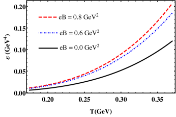
Figure 1: Energy density for different magnetic fields as a function of temperature.

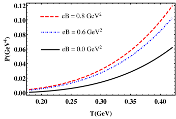
Figure 2: Pressure for different magnetic fields as a function of temperature.

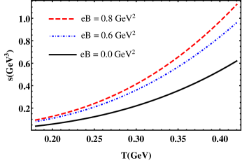
Figure 3: Entropy density for different magnetic fields as a function of temperature.

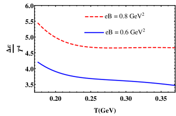
Figure 4: ${\Delta\varepsilon}/{T^{4}}$ for two different magnetic fields, plotted as a function of temperature.

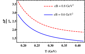
Figure 5: ${\Delta P}/{T^{4}}$ for two different magnetic fields, plotted as a function of temperature.

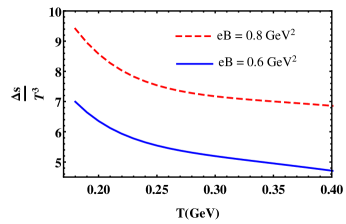
Figure 6: ${\Delta s}/{T^{3}}$ for two different magnetic fields, plotted as a function of temperature.

We have shown the temperature dependence of different thermodynamic quantities at different values of magnetic fields in Figs. 1-3. Fig.1 shows that the energy density increases, at a given temperature, as the magnetic field increases. This is expected as, in the presence of magnetic field the total energy density goes as $\varepsilon_{total}=\varepsilon+q\textbf{M}\cdot\textbf{B}$, where M is the magnetization Kurian and Chandra (2017). We notice that the plots show correct qualitative behaviour. The quark/gluon contribution to the thermodynamic pressure, energy density, and entropy density increase with the increase in $eB$. This behaviour is consistent with that obtained using lattice QCD simulations Bali et al. (2014) and Levkova and DeTar (2014). The same behaviour has been obtained using an effective fugacity quasiparticle model in Kurian and Chandra (2017), within SU(2) NJL model in Farias et al. (2017) and using the Bag Model in Fraga and Palhares (2012). There are several other studies which study magnetised quark matter. The QCD equation of state in the presence of magnetic field has been studied numerically in Bonati et al. (2013, 2014). The effect of magnetic field on QCD thermodynamics has been studied using the HTL perturbation theory both at strongRath and Patra (2017) and in weak Bandyopadhyay et al. magnetic fields.

$\Delta\varepsilon$ is the difference between energy density in the presence of magnetic fields with that in the absence of any magnetic field. This depicts the increment of energy density in the presence of the magnetic field. The temperature dependence of $\Delta\varepsilon/T$ has been plotted in Fig.3. In addition, we have plotted ${\Delta P}/{T^{4}}$ and ${\Delta s}/{T^{3}}$ as functions of temperature. As expected, higher the magnetic field, higher are their values too.

The transverse pressure can be obtained using equation (32) and (33). The calculation involves taking the derivatives with respect to the magnetic field. We are not able to calculate it here because the functional dependence of the coupling constant on the magnetic field in equation (43) is unknown. We emphasize that this is not a shortcoming of our model and that with the knowledge of the exact functional dependence of the coupling constant on the magnetic field we will be able to calculate the transverse pressure too.

IV Conclusions

We have extended the self-consistent quasiparticle model for hot QCD in the presence of magnetic fields to understand the behaviour of magnetised quark matter. The effect of magnetic fields has been included by redefining the thermal mass of quasiparticles. The definition of thermal mass in the self-consistent model has been extended to define a thermo-magnetic mass through Landau Level quantisation for fermions. The thermodynamic quantities are evaluated by starting with the modified momentum distributions and the energy dispersion relations. The modification of these quantities has been brought about by incorporating relativistic Landau Levels.

Using this modified quasiparticle model, we have studied the $2$-flavor system in the temperature range $170$-$400$ MeV, in the presence of magnetic fields. To this end, we made use of a parametrisation of the coupling constant that depends both on temperature and magnetic field, obtained in the context of $SU(2)$ NJL model. We found that the energy density, pressure and entropy density increase in the presence of a magnetic field as expected. Our results are qualitatively consistent with the results obtained using other approaches including lattice QCD simulations.

The correct behaviour of the equation of state shows that the self-consistent quasiparticle model can be extended to study the thermodynamics of quark-gluon plasma in the presence of magnetic fields. For a quantitative study that can be compared with the lattice data, we need a coupling constant depending both on temperature and magnetic field. With a proper parametrisation of the coupling constant for $2+1$ flavor, we can easily extend this work to obtain the equation of state for $2+1$ flavor QGP in the presence of magnetic field and also calculate the transverse components of pressure. We intend to do this in our future work. Another area that we plan to investigate further is how the modified equation of state affects the transport coefficients of QGP.

V Acknowledgements

One of the authors Sebastian Koothottil would like to thank Manu Kurian for the helpful discussions, Arjun K. for helping with calculations and R. L. S. Farias for his comments and suggestions. Sebastian Koothottil would also like to thank UGC BSR SAP for providing research fellowship during the period of research.

References

- Back et al. (2005) B. Back et al., Nuclear Physics A 757, 28 (2005), first Three Years of Operation of RHIC.
- Adams et al. (2005) J. Adams et al., Nuclear Physics A 757, 102 (2005), first Three Years of Operation of RHIC.
- Adcox et al. (2005) K. Adcox et al., Nuclear Physics A 757, 184 (2005), first Three Years of Operation of RHIC.
- Arsene et al. (2005) I. Arsene et al., Nuclear Physics A 757, 1 (2005), first Three Years of Operation of RHIC.
- SKOKOV et al. (2009) V. V. SKOKOV, A. Y. ILLARIONOV, and V. D. TONEEV, International Journal of Modern Physics A 24, 5925 (2009).
- Yang et al. (2015) Z. Yang, Y. Chun-Bin, C. Xu, and F. Sheng-Qin, Chinese Physics C 39, 104105 (2015).
- Tuchin (2011) K. Tuchin, Phys. Rev. C 83, 017901 (2011).
- Marasinghe and Tuchin (2011) K. Marasinghe and K. Tuchin, Phys. Rev. C 84, 044908 (2011).
- Tuchin (2010) K. Tuchin, Phys. Rev. C 82, 034904 (2010).
- Fukushima and Pawlowski (2012) K. Fukushima and J. M. Pawlowski, Phys. Rev. D 86, 076013 (2012).
- Gusynin et al. (1994) V. Gusynin, V. Miransky, and I. Shovkovy, Physical Review Letters 73, 3499 (1994).
- cat (2013) Strongly Interacting Matter in Magnetic Fields (Springer Berlin Heidelberg, 2013).
- Gusynin et al. (1996) V. Gusynin, V. Miransky, and I. Shovkovy, Nuclear Physics B 462, 249 (1996).
- Fukushima and Hidaka (2013) K. Fukushima and Y. Hidaka, Physical Review Letters 110 (2013), 10.1103/physrevlett.110.031601.
- Fukushima et al. (2008) K. Fukushima, D. E. Kharzeev, and H. J. Warringa, Phys. Rev. D 78, 074033 (2008).
- Kharzeev et al. (2008) D. E. Kharzeev, L. D. McLerran, and H. J. Warringa, Nuclear Physics A 803, 227 (2008).
- Kharzeev (2014) D. E. Kharzeev, Progress in Particle and Nuclear Physics 75, 133 (2014).
- Grasso and Rubinstein (2001) D. Grasso and H. R. Rubinstein, Physics Reports 348, 163 (2001).
- Duncan and Thompson (1992) R. C. Duncan and C. Thompson, The Astrophysical Journal 392, L9 (1992).
- Broderick et al. (2000) A. Broderick, M. Prakash, and J. M. Lattimer, The Astrophysical Journal 537, 351 (2000).
- Cardall et al. (2001) C. Y. Cardall, M. Prakash, and J. M. Lattimer, The Astrophysical Journal 554, 322 (2001).
- Rabhi et al. (2008) A. Rabhi, C. Providência, and J. D. Providência, Journal of Physics G: Nuclear and Particle Physics 35, 125201 (2008).
- Rabhi et al. (2011) A. Rabhi, P. K. Panda, and C. Providência, Physical Review C 84 (2011), 10.1103/physrevc.84.035803.
- Strickland et al. (2012) M. Strickland, V. Dexheimer, and D. P. Menezes, Physical Review D 86 (2012), 10.1103/physrevd.86.125032.
- Avancini et al. (2018) S. S. Avancini, V. Dexheimer, R. L. S. Farias, and V. S. Timóteo, Physical Review C 97 (2018), 10.1103/physrevc.97.035207.
- Kurian and Chandra (2018) M. Kurian and V. Chandra, Physical Review D 97 (2018), 10.1103/physrevd.97.116008.
- (27) M. Kurian, S. Mitra, and V. Chandra, http://arxiv.org/abs/1805.07313v1 .
- Goloviznin and Satz (1993) V. Goloviznin and H. Satz, Zeitschrift für Physik C Particles and Fields 57, 671 (1993).
- Peshier et al. (1994) A. Peshier, B. Kämpfer, O. Pavlenko, and G. Soff, Physics Letters B 337, 235 (1994).
- Dumitru and Pisarski (2002) A. Dumitru and R. D. Pisarski, Physics Letters B 525, 95 (2002).
- Fukushima (2004) K. Fukushima, Physics Letters B 591, 277 (2004).
- Ghosh et al. (2006) S. K. Ghosh, T. K. Mukherjee, M. G. Mustafa, and R. Ray, Physical Review D 73 (2006), 10.1103/physrevd.73.114007.
- Abuki and Fukushima (2009) H. Abuki and K. Fukushima, Physics Letters B 676, 57 (2009).
- Tsai and Müller (2009) H.-M. Tsai and B. Müller, Journal of Physics G: Nuclear and Particle Physics 36, 075101 (2009).
- D’Elia et al. (1997) M. D’Elia, A. D. Giacomo, and E. Meggiolaro, Physics Letters B 408, 315 (1997).
- Castorina and Mannarelli (2007a) P. Castorina and M. Mannarelli, Physics Letters B 644, 336 (2007a).
- Castorina and Mannarelli (2007b) P. Castorina and M. Mannarelli, Physical Review C 75 (2007b), 10.1103/physrevc.75.054901.
- Su and Tywoniuk (2015) N. Su and K. Tywoniuk, Physical Review Letters 114 (2015), 10.1103/physrevlett.114.161601.
- Bannur (2007a) V. M. Bannur, Physical Review C 75 (2007a), 10.1103/physrevc.75.044905.
- Bannur (2007b) V. M. Bannur, Physics Letters B 647, 271 (2007b).
- Bannur (2007c) V. M. Bannur, Journal of High Energy Physics 2007, 046 (2007c).
- Bannur (2007d) V. M. Bannur, The European Physical Journal C 50, 629 (2007d).
- Bannur (2008) V. M. Bannur, Physical Review C 78 (2008), 10.1103/physrevc.78.045206.
- Chandra and Ravishankar (2009) V. Chandra and V. Ravishankar, The European Physical Journal C 64, 63 (2009).
- Chandra and Ravishankar (2011) V. Chandra and V. Ravishankar, Physical Review D 84 (2011), 10.1103/physrevd.84.074013.
- Pisarski (1989) R. D. Pisarski, Physical Review Letters 63, 1129 (1989).
- Pisarski (1993) R. D. Pisarski, Physical Review D 47, 5589 (1993).
- Peshier et al. (1996) A. Peshier, B. Kämpfer, O. P. Pavlenko, and G. Soff, Physical Review D 54, 2399 (1996).
- Medvedev (1999) M. V. Medvedev, Physical Review E 59, R4766 (1999).
- Bannur (2006) V. M. Bannur, Physical Review E 73 (2006), 10.1103/physreve.73.067401.
- Bannur (2012) V. M. Bannur, International Journal of Modern Physics E 21, 1250090 (2012).
- (52) K. Bhattacharya, http://arxiv.org/abs/0705.4275v2 .
- Bruckmann et al. (2018) F. Bruckmann, G. Endrődi, M. Giordano, S. D. Katz, T. G. Kovács, F. Pittler, and J. Wellnhofer, EPJ Web of Conferences 175, 07014 (2018).
- Fraga and Palhares (2012) E. S. Fraga and L. F. Palhares, Physical Review D 86 (2012), 10.1103/physrevd.86.016008.
- Mizher et al. (2010) A. J. Mizher, M. N. Chernodub, and E. S. Fraga, Physical Review D 82 (2010), 10.1103/physrevd.82.105016.
- Chakrabarty (1996) S. Chakrabarty, Physical Review D 54, 1306 (1996).
- Bruckmann et al. (2017) F. Bruckmann, G. Endrődi, M. Giordano, S. Katz, T. Kovács, F. Pittler, and J. Wellnhofer, Physical Review D 96 (2017), 10.1103/physrevd.96.074506.
- Tawfik (2016) A. N. Tawfik, Journal of Physics: Conference Series 668, 012082 (2016).
- KOHRI et al. (2004) K. KOHRI, S. YAMADA, and S. NAGATAKI, Astroparticle Physics 21, 433 (2004).
- Ferrer et al. (2010) E. J. Ferrer, V. de la Incera, J. P. Keith, I. Portillo, and P. L. Springsteen, Physical Review C 82 (2010), 10.1103/physrevc.82.065802.
- Martínez et al. (2003) A. P. Martínez, H. P. Rojas, and H. J. M. Cuesta, The European Physical Journal C 29, 111 (2003).
- Chaichian et al. (2000) M. Chaichian, S. S. Masood, C. Montonen, A. P. Martínez, and H. P. Rojas, Physical Review Letters 84, 5261 (2000).
- Potekhin and Yakovlev (2012) A. Y. Potekhin and D. G. Yakovlev, Physical Review C 85 (2012), 10.1103/physrevc.85.039801.
- Ferrer et al. (2012) E. J. Ferrer, V. de la Incera, J. P. Keith, I. Portillo, and P. L. Springsteen, Physical Review C 85 (2012), 10.1103/physrevc.85.039802.
- Dexheimer et al. (2013) V. Dexheimer, D. P. Menezes, and M. Strickland, Journal of Physics G: Nuclear and Particle Physics 41, 015203 (2013).
- Bali et al. (2014) G. S. Bali, F. Bruckmann, G. Endrödi, S. D. Katz, and A. Schäfer, Journal of High Energy Physics 2014 (2014), 10.1007/jhep08(2014)177.
- Bali et al. (2013) G. S. Bali, F. Bruckmann, G. Endrődi, F. Gruber, and A. Schäfer, Journal of High Energy Physics 2013 (2013), 10.1007/jhep04(2013)130.
- Blandford and Hernquist (1982) R. D. Blandford and L. Hernquist, Journal of Physics C: Solid State Physics 15, 6233 (1982).
- Menezes et al. (2009) D. P. Menezes, M. B. Pinto, S. S. Avancini, A. P. Martínez, and C. Providência, Physical Review C 79 (2009), 10.1103/physrevc.79.035807.
- Ferrer et al. (2015) E. Ferrer, V. de la Incera, and X. Wen, Physical Review D 91 (2015), 10.1103/physrevd.91.054006.
- Ayala et al. (2018) A. Ayala, C. Dominguez, S. Hernandez-Ortiz, L. Hernandez, M. Loewe, D. M. Paret, and R. Zamora, Physical Review D 98 (2018), 10.1103/physrevd.98.031501.
- Miransky and Shovkovy (2002) V. A. Miransky and I. A. Shovkovy, Physical Review D 66 (2002), 10.1103/physrevd.66.045006.
- Ferreira et al. (2014) M. Ferreira, P. Costa, O. Lourenço, T. Frederico, and C. Providência, Physical Review D 89 (2014), 10.1103/physrevd.89.116011.
- Farias et al. (2014) R. L. S. Farias, K. P. Gomes, G. Krein, and M. B. Pinto, Physical Review C 90 (2014), 10.1103/physrevc.90.025203.
- Farias et al. (2017) R. L. S. Farias, V. S. Timóteo, S. S. Avancini, M. B. Pinto, and G. Krein, The European Physical Journal A 53 (2017), 10.1140/epja/i2017-12320-8.
- Kurian and Chandra (2017) M. Kurian and V. Chandra, Physical Review D 96 (2017), 10.1103/physrevd.96.114026.
- Levkova and DeTar (2014) L. Levkova and C. DeTar, Physical Review Letters 112 (2014), 10.1103/physrevlett.112.012002.
- Bonati et al. (2013) C. Bonati, M. D’Elia, M. Mariti, F. Negro, and F. Sanfilippo, Physical Review Letters 111 (2013), 10.1103/physrevlett.111.182001.
- Bonati et al. (2014) C. Bonati, M. D’Elia, M. Mariti, F. Negro, and F. Sanfilippo, Physical Review D 89 (2014), 10.1103/physrevd.89.054506.
- Rath and Patra (2017) S. Rath and B. K. Patra, Journal of High Energy Physics 2017 (2017), 10.1007/jhep12(2017)098.
- (81) A. Bandyopadhyay, B. Karmakar, N. Haque, and M. G. Mustafa, http://arxiv.org/abs/1702.02875v2 .