Resurgence Analysis of Quantum Invariants of Seifert Fibered Homology Spheres

Abstract

For a Seifert fibered homology sphere $X$ we show that the $q$-series invariant $\hat{\operatorname{Z}}_{0}(X;q)$ introduced by Gukov-Pei-Putrov-Vafa, is a resummation of the Ohtsuki series $\operatorname{Z}_{0}(X)$. We show that for every even $k\in\mathbb{N}$ there exists a full asymptotic expansion of $\hat{\operatorname{Z}}_{0}(X;q)$ for $q$ tending to $e^{2\pi i/k}$, and in particular that the limit $\hat{\operatorname{Z}}_{0}(X;e^{2\pi i/k})$ exists and is equal to the WRT quantum invariant $\tau_{k}(X)$. We show that the poles of the Borel transform of $\operatorname{Z}_{0}(X)$ coincide with the classical complex Chern-Simons values, which we further show classifies the corresponding components of the moduli space of flat $\rm{SL}(2,\mathbb{C})$-connections.

Introduction

Let $X$ be a closed and oriented $3$-manifold and consider the level $k$ Witten-Reshetikhin-Turaev quantum invariant [48, 49]

$$\tau_{k}(X)\in\mathbb{C},k\in\mathbb{N}.$$ (1)

In [29] Gukov, Pei, Putrov and Vafa proposed the existence of an invariant of $(X,a)$, $a\in\operatorname{Spin^{c}}(X),$ which is an integer power series convergent inside the unit disc

$$\hat{\operatorname{Z}}_{a}(X;q)\in 2^{-c}q^{\Delta}\mathbb{Z}[[q]].$$ (2)

In [27], $\hat{\operatorname{Z}}_{a}(X;q)$ was conceived as a resummation of the asymptotic expansion of $\tau_{k}(X)$. The radial limit conjecture [12, 28, 29] postulates that the following limits exists

$$\hat{\operatorname{Z}}_{a}(X,e^{2\pi i/k})=\lim_{q\uparrow e^{2\pi i/k}}\hat{\operatorname{Z}}_{a}(X,q)$$

and that these limits recovers $\tau_{k}(X)$ through an $S$-transform.

We now summarize the main results of this paper. Let $p_{1},...,p_{n}\in\mathbb{N}$ be pairwise coprime integers, and let for the rest of this paper $X$ denote the oriented Seifert fibered homology sphere with $n\geq 3$ exceptional fibers

$$X=\Sigma(p_{1},...,p_{n}).$$ (3)

Let $\mathcal{M}(G)=\mathcal{M}(X,G)$ be the moduli space of flat $G$-connections, let $\operatorname{S_{CS}}$ be the Chern-Simons action and let $\operatorname{Z}_{0}=\operatorname{Z}_{0}(X)$ be the Ohtsuki series. Denote the set of classical complex Chern-Simons values by

$$\operatorname{CS}_{\mathbb{C}}(X)=\operatorname{S_{CS}}(\mathcal{M}(\operatorname{SL}(2,\mathbb{C}))).$$

• Theorem 1 computes $\operatorname{CS}_{\mathbb{C}}(X)$, establishes that $\operatorname{S_{CS}}$ is injective on $\pi_{0}(\mathcal{M}(\operatorname{SL}(2,\mathbb{C})))$ and that

  $$\pi_{0}(\mathcal{M}(\operatorname{SL}(2,\mathbb{R}))\sqcup_{\mathcal{M}(\text{U}(1))}\mathcal{M}(\operatorname{SU}(2)))\cong\pi_{0}(\mathcal{M}(\operatorname{SL}(2,\mathbb{C}))).$$

• Theorem 2 establishes that $\operatorname{CS}_{\mathbb{C}}(X)$ coincide with the poles of the Borel transform of $\operatorname{Z}_{0}(X)$.

• Theorem 3 establishes that $\hat{\operatorname{Z}}_{0}(X;q)$ is a Borel-Laplace resummation of $\operatorname{Z}_{0}(X)$.

• Theorem 4 establishes that $\hat{\operatorname{Z}}_{0}(X;q)$ admits a full asymptotic expansion for $q\rightarrow e^{2\pi i/k}$, and that the radial limit conjecture is true for $X$.

We now present these results in full detail.

Complex Chern-Simons Theory on $X$

For a rational number $x\in\mathbb{Q}$ let $[x]=x\mod\mathbb{Z}.$ We prove

Theorem 1.

The Chern-Simons action $\operatorname{S_{CS}}$ is injective on $\pi_{0}(\mathcal{M}(\operatorname{SL}(2,\mathbb{C})))$ and we have

$$\operatorname{CS}_{\mathbb{C}}(X)=\{[0]\}\sqcup\left\{\left[\frac{-m^{2}}{4P}\right]:\text{ $m\in\mathbb{Z}$ is divisible by at most $n-3$ of the $p_{j}$'s}\right\}.$$ (4)

The natural inclusion $\mathcal{M}(\operatorname{SL}(2,\mathbb{R}))\sqcup_{\mathcal{M}(\text{U}(1))}\mathcal{M}(\operatorname{SU}(2))\rightarrow\mathcal{M}(\operatorname{SL}(2,\mathbb{C}))$ induces an isomorphism on the level of $\pi_{0}$

$$\pi_{0}(\mathcal{M}(\operatorname{SL}(2,\mathbb{R}))\sqcup_{\mathcal{M}(\text{U}(1))}\mathcal{M}(\operatorname{SU}(2)))\cong\pi_{0}(\mathcal{M}(\operatorname{SL}(2,\mathbb{C}))).$$

The Borel transform and Complex Chern-Simons

Set $P=\prod_{j=1}^{n}p_{j}.$ For $k\in\mathbb{N}^{*}$ set $q_{k}=\exp(2\pi i/k)$ and let $\varsigma\in\mathbb{C}^{*}$ and $\phi\in\mathbb{Q}$ be the constants introduced below in (23). We consider the normalized quantum invariant

$$\widetilde{\operatorname{Z}}_{k}(X)=\varsigma q_{k}^{\frac{\phi}{4}}\frac{\tau_{k}(X)}{\tau_{k}(\operatorname{S}^{2}\times\operatorname{S}^{1})}.$$ (5)

Let $\operatorname{CS}^{*}(X)=\operatorname{CS}(X)\setminus\{[0]\}$. Introduce the rational function

$$G(z)=\prod_{j=1}^{n}\left(z^{\frac{P}{p_{j}}}-z^{-\frac{P}{p_{j}}}\right)\left(z^{P}-z^{-P}\right)^{2-n}.$$ (6)

In Theorem 2 we use the notion of a resurgent function and the Borel transform, which are recalled below in Definitions 2 and 218 respectively. Let $\kappa=\sqrt{2\pi iP}.$ Building on the work of Lawrence and Rozansky [39] we prove the following

Theorem 2.

There are uniquely determined polynomials $\operatorname{Z}_{\theta}=\operatorname{Z}_{\theta}(X)$ for $\theta\in\operatorname{CS}^{*}_{\mathbb{C}}(X)\}$ of degree at most $n-3$ and a formal power series $\operatorname{Z}_{0}=\operatorname{Z}_{0}(X)\in x^{-\frac{1}{2}}\mathbb{C}[[x^{-1}]]$ giving the full asymptotic expansion in the Poincare sense

$$\widetilde{\operatorname{Z}}_{k}(X)\sim_{k\rightarrow\infty}\sum_{\theta\in\operatorname{CS}_{\mathbb{C}}(X)}e^{2\pi ik\theta}\operatorname{Z}_{\theta}(k).$$ (7)

The series $\operatorname{Z}_{0}$ is a normalization of the Ohtsuki series of $X$ (see Equation (30)) whose Borel transform $\mathcal{B}(\operatorname{Z}_{0})$ is the resurgent function

$$\mathcal{B}(\operatorname{Z}_{0})(\zeta)=\frac{\kappa}{\pi i\sqrt{\zeta}}G\left(\exp\left(\frac{\kappa\sqrt{\zeta}}{P}\right)\right)=\frac{\kappa i}{4\pi}\frac{\prod_{j=1}^{n}\sinh\left(\frac{\kappa\sqrt{\zeta}}{p_{j}}\right)}{\sqrt{\zeta}\left(\sinh\left(\kappa\sqrt{\zeta}\right)\right)^{n-2}},$$ (8)

and if $\Omega$ is the set of poles of $\mathcal{B}(\operatorname{Z}_{0})$, then

$$\Omega=-2\pi i\operatorname{CS}_{\mathbb{C}}^{*}(X)+2\pi i\mathbb{Z}.$$ (9)

Remark 1.

In accordance with the asymptotic expansion conjecture (formulated by the first author in [1], and proven in our joint work [5] for generic mapping tori and by the first author et al. in [4] for finite order mapping tori with links s and further proven by Marche and Charles for certain surgeries on the figure 8 knot in [11]), we expect that the sum in (7) should only range over the Chern-Simons values of flat $\operatorname{SU}(2)$-connections

$$\operatorname{CS}(X)=\operatorname{S_{CS}}(\mathcal{M}(X,\operatorname{SU}(2))),$$

e.g. that the terms which does not correspond to such values in the sum in (7) vanishes. This is known to be true for $n=3$ [34] and in some cases for $n=4$ [33]. However we see from (9) that the quantum invariants via resurgence determines all the Chern-Simons values of flat $\operatorname{SL}(2,\mathbb{C})$-connections.

A resurgence formula for the GPPV invariant $\mathbf{\hat{\operatorname{Z}}}$

Let $\Delta\in\mathbb{Q}$ be given by Equation (113) and consider the GPPV invariant

$$\hat{\operatorname{Z}}_{0}(X;q)\in q^{-\Delta}\mathbb{Z}[[q]].$$ (10)

We recall the definition of $\hat{\operatorname{Z}}_{0}(X;q)$ from [29, 28] and recall that it is convergent for $\lvert q\rvert<1$.

Set $m_{0}=P(n-2-\sum_{j=1}^{n}p_{j}^{-1})\in\mathbb{Z}.$ There exists a sequence of integers $\{\chi_{m}\}_{m=m_{0}}^{\infty}$ such that for all $z\in\mathbb{C}$ with $\lvert z\rvert<1$

$$G(z)=(-1)^{n}\sum_{m=m_{0}}^{\infty}\chi_{m}z^{m}\in\mathbb{Z}[[z]].$$ (11)

Let $\mathfrak{h}$ denote the upper half-plane. Let $\tau\in\mathfrak{h}$ and set $q=\exp(2\pi i\tau)$ and $\lambda=(-1)^{n}\frac{i}{2}(2P)^{-1/2}.$ Let $\varGamma=\varGamma_{+}+\varGamma_{-}$ be the oriented unbounded contour depicted in Figure 1. We show that the GPPV invariant $\hat{\operatorname{Z}}_{0}(X;q)$ is a resummation (see Appendix A) of the Ohtsuki series $\operatorname{Z}_{0}(X)$.

Theorem 3.

$$q^{\Delta}\hat{\operatorname{Z}}_{0}(X;q)=\frac{\lambda}{\sqrt{\tau}}\int_{\varGamma}\exp(-\zeta/\tau)\mathcal{B}(\operatorname{Z}_{0}(X))(\zeta)\operatorname{{d}\hskip-1.70717pt}\zeta=\sum_{m=m_{0}}^{\infty}\chi_{m}q^{\frac{m^{2}}{4P}}.$$ (12)

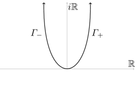
Figure 1: The integration contour $\varGamma=\varGamma_{+}+\varGamma_{-}.$

The asymptotic expansion of the GPPV invariant $\hat{\operatorname{Z}}$

We now turn to the asymptotic expansion of $\hat{\operatorname{Z}}_{0}(X)$ and the radial limit conjecture [12, 28, 29], which is recalled in Conjecture 2. Assume that $P$ is even. Set $\delta=\Delta-\phi/4$ and $\mu=(2\lambda\varsigma)^{-1}$. For a positive parameter $t$ set

$$q_{k,t}=\exp\left(\frac{2\pi i}{k-i\frac{2Pt}{\pi}}\right)\in\mathfrak{h}.$$ (13)

Theorem 4.

For each $\theta\in\operatorname{CS}^{*}_{\mathbb{C}}(X)$ there exists a unique polynomial (defined in (187)) in $k$ of degree at most $n-3$ with coefficients in formal power series without constant terms

$$\check{\operatorname{Z}}_{\theta}(k,t)\in t\cdot\mathbb{Q}[\pi i,k][[t]]$$ (14)

giving a full Poincare asymptotic expansion for small $t$ and fixed even $k$

$$(\sqrt{k}\lambda)^{-1}q_{k,t}^{\Delta}\hat{\operatorname{Z}}_{0}(X;q_{k,t})\ \underset{t\rightarrow 0}{\sim}\ \tilde{\operatorname{Z}}_{k}(X)+\sum_{\theta\in\operatorname{CS}^{*}_{\mathbb{C}}(X)}e^{2\pi ik\theta}\check{\operatorname{Z}}_{\theta}(k,t).$$ (15)

In particular, for every even $k$ we have

$$\frac{\mu}{\sqrt{k}}\lim_{q\uparrow q_{k,0}}q^{\delta}\hat{\operatorname{Z}}_{0}(X;q)=\frac{\tau_{k}(X)}{\tau_{k}(\operatorname{S}^{2}\times\operatorname{S}^{1})}.$$ (16)

Thus the radial limit conjecture (Conjecture 2) holds for $X$.

Comparisons with the literature

The existence of an asymptotic expansion

$$\widetilde{\operatorname{Z}}_{k}(X)\sim_{k\rightarrow\infty}\sum_{\theta\in R(Y)}e^{2\pi ik\theta}\operatorname{Z}_{\theta}(k)$$ (17)

where $R(Y)\subset\mathbb{Q}/\mathbb{Z}$ is a finite set was proven in [39]. In this work, it was also shown that $\operatorname{Z}_{0}$ is a normalization of the Ohtsuki series. Our contribution in regard to (17) is to compute $\operatorname{CS}_{\mathbb{C}}(X)$ and to show $R(X)\subset\operatorname{CS}_{\mathbb{C}}(X).$ In [39] the authors do not adress the Borel transform of $\operatorname{Z}_{0}$.

The $q$-series from Theorem 3

$$\Psi(q)=\sum_{m=m_{0}}^{\infty}\chi_{m}q^{\frac{m^{2}}{4P}}\in\mathbb{Z}[[q^{\frac{1}{4P}}]]$$ (18)

was considered in the study of $\tau_{k}(\Sigma(p_{1},p_{2},p_{3}))$ by Lawrence and Zagier [40], and further explored by Hikami [33]. For $n\geq 4$ Hikami in [34] considers a differently defined $q$-series. Our Theorem 4 generalize the result from [40].

The work [27] of Gukov, Marino and Putrov is one of the main inspirations for this paper. In [27] the authors analyse $\tau_{k}(X)$ for some examples with $n=3.$ The identity (9) was verified for these examples. For $\tau\in\mathfrak{h}$ set $h=2\pi i\tau$ so that $q=\exp(h)$. Consider again the countor integral

$$\operatorname{I}(h)=\frac{\lambda}{\sqrt{\tau}}\int_{\varGamma}\exp\left(-\frac{2\pi i\xi}{h}\right)\mathcal{B}(\operatorname{Z}_{0})(\xi)\ \operatorname{{d}\hskip-1.70717pt}\xi.$$ (19)

In [27] identities of the form

$$\operatorname{I}(h)=\Psi(q)$$ (20)

where discovered. In a sense, the series $\Psi(q)$ was taken as a definition for $\hat{\operatorname{Z}}_{0}(q)$ for $\Sigma(p_{1},p_{2},p_{3})$, and the GPPV-formula (Definition 1) was only later introduced in [29].

In the work [25] of Fuji, Iwaki, Murakami and Terashima the $q$-series $\Psi(q)$ is also considered for general $n\geq 3$, and they prove a radial limit theorem, which is analogous to (16). The also prove an identity of the form (20). In [25] they do not however work with the definition of the GPPV invariant $\hat{\operatorname{Z}}_{0}(q)$, although they conjecture that this is equal to $\Psi(q)$. They also consider the case of the WRT invariant of a knot inside $X$ and prove a difference equation for $\Psi(q)$.

Our Theorem 3 shows

$$q^{\Delta}\hat{\operatorname{Z}}_{0}(q)=\operatorname{I}(h)=\Psi(q)$$

for all Seifert fibered integral homology $3$-spheres $X$ with $n\geq 3$ singular fibers, where $\hat{\operatorname{Z}}_{0}(q)$ is independently defined via the GPPV-formula. We remark that those of our results that overlap with [25] had been presented prior to their submission by the first name author in the online seminar [2] and by the second author at a seminar [42] at IST, Austria. The $q$-series $\Psi(q)$ was also conjectured to be a normalization of $\hat{\operatorname{Z}}_{0}(q)$ in the second author’s thesis [41] . We also remark that our proof of the radial limit formula (16) differs from theirs; our stronger Theorem 4 is derived using the resurgence formula for $\hat{\operatorname{Z}}_{0}(q)$ from Theorem 3, whilst their proof of their radial limit theorem uses Gaussian reciprocity directly on $\Psi(q)$. We warmly thank them for cordial coordination.

Acknowledgements

We warmly thank S. Gukov for valuable discussions on the invariant $\hat{\operatorname{Z}}_{a}(q).$

Organization

In Section 1 we prove Theorem 1 in several steps. Theorem 6 gives a decomposition of the moduli space, Corollary 8 computes the Chern-Simons invariants and Theorem 9 proves that components of this moduli space are classified by their Chern-Simons value. In Section 2 we prove Theorem 2. Corollary 10 gives a resurgence formula for $\tilde{\operatorname{Z}}_{k}(X)$, and Proposition 11 gives an exact formula for its generating function, verifying a special case of a conjecture of Garoufalidis [26]. In Section 3 we prove Theorem 3 and in Section 4 we prove Theorem 4. In Appendix A we present the definition of a resurgent function and the definition of the Borel transform, as well as some generalities on the relation between the Borel transform and the Laplace transform used in this paper.

1 Complex Chern-Simons theory on $X$

Let $X$ be the oriented Seifert fibered homology $3$-sphere from the introduction. Choose $q_{1},...,q_{n}\in\mathbb{Z}$ such that $(p_{j},q_{j})=1$ and

$$\sum_{j=1}^{n}\frac{q_{j}}{p_{j}}=\frac{1}{P}.$$ (21)

Then $X$ has a surgery diagram as depicted in Figure 2 below.

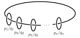
Figure 2: Surgery link for $X.$

Without loss of generality we can assume that $p_{2},...,p_{n}$ are odd. The homeomorphism type of $X$ is unaltered under a transformation $q_{j}\mapsto q_{j}+y_{j}$ for any choice of integers $y_{1},...,y_{n}$ such that $(p_{j},q_{j}+y_{j})=1$ and

$$\sum_{j=1}^{n}\frac{q_{j}}{p_{j}}=\sum_{j=1}\frac{q_{j}+y_{j}}{p_{j}}.$$ (22)

If $q_{j}$ is odd for $j>1$, we perform the transformation $q_{j}\mapsto q_{j}+p_{j}$ and $q_{1}\mapsto q_{1}-(n-1)p_{1}$ which does not change the sum (22). Hence we can assume without loss of generality that $q_{2},...,q_{n}$ are all even. Recall that under our assumptions $1=P\sum_{j=1}\frac{q_{j}}{pj}.$ Note that this implies that $q_{1}$ is odd.

We recall the computation of $\tau_{k}(X)$ from [39]. Let $S({}\cdot{},{}\cdot{})$ be the Dedekind sum. Introduce the constants

$$\varsigma=-\frac{\sqrt{P}}{4}\exp\left(-\frac{\pi i3}{4}\right), \phi=3-\frac{1}{P}+12\sum_{j=1}^{n}S\left(\frac{P}{p_{j}},p_{j}\right).$$ (23)

The quantity $\phi$ is related to the Casson-Walker invariant $\lambda(X)$ [51] (in Casson’s normalization) as follows

$$-24\lambda(X)=\phi+P\left(n-2-\sum_{j=1}^{n}p_{j}^{-2}\right).$$

Define the meromorphic function $F\in\mathcal{M}(\mathbb{C})$ and $g\in\mathbb{C}[y]$ explicitly as follows

$$\begin{split}F(y&)=\frac{1}{4}\left(\sinh\left(\frac{y}{2}\right)\right)^{2-n}\prod_{j=1}^{n}\sinh\left(\frac{y}{2p_{j}}\right),\\ g(y)&=\frac{iy^{2}}{8\pi P}.\end{split}$$ (24)

Lawrence and Rozansky shows in [39] the following results. There exists a finite subset $R^{*}(X)\subset\mathbb{Q}^{*}/\mathbb{Z}$ and non-vanishing polynomials $\operatorname{Z}_{\theta}(z)\in\mathbb{C}[z]$, $\theta\in R^{*}(X)$ of degree at most $n-3$ such that

$$\sum_{\theta\in R^{*}(X)}e^{2\pi ik\theta}\operatorname{Z}_{\theta}(k)=-\sum_{m=1}^{2P-1}\text{Res}\left(\frac{F(y)e^{kg(y)}}{1-e^{-ky}},y=2\pi im\right)$$ (25)

for all non-negative integers $k$. Let $\gamma$ to be the contour from $(-1-i)\infty$ to $(1+i)\infty$. Observe that $\gamma(H)$ is a steepest descent path for $g.$ Introduce the following notation

$$\begin{split}\operatorname{Z}^{R}(k)&=\sum_{\theta\in R^{*}(X)}e^{2\pi ik\theta}\operatorname{Z}_{\theta}(k)\\ \operatorname{Z}^{\operatorname{I}}(k)&=\frac{1}{2\pi i}\int_{\gamma}F(y)e^{kg(y)}\ \operatorname{{d}\hskip-1.70717pt}y.\end{split}$$ (26)

Recalling the definition of the normalized quantum invariant $\widetilde{\operatorname{Z}}_{k}$ given in (5), Lawrence and Rozansky proved that it can be decomposed into a sum of an integral part $\operatorname{Z}^{\operatorname{I}}$ and a residue part $\operatorname{Z}^{R}$

$$\widetilde{\operatorname{Z}}_{k}(X)=\operatorname{Z}^{\operatorname{I}}(k)+\operatorname{Z}^{R}(k).$$ (27)

This is Equation $4.8$ on in Section $4.5$ in [39]. We have used the same notation for $F,g$ and $\phi$ whereas the constant $B$ in their notation is equal to $\varsigma^{-1}$. Thus, if we define

$$\operatorname{Z}_{0}(x)=\frac{1}{2\pi i}\sqrt{P\pi i8}\sum_{n=0}^{\infty}\frac{F^{(2n)}(0)\left(i8P\pi\right)^{n}}{(2n)!}\frac{\Gamma\left(n+\frac{1}{2}\right)}{x^{n+\frac{1}{2}}}\in\ x^{-1/2}\mathbb{C}[[x^{-1}]]$$ (28)

and set $R(X)=R^{*}(X)\sqcup\{0\}$ then we have an asymptotic expansion

$$\widetilde{\operatorname{Z}}_{k}(X)\sim_{k\rightarrow\infty}\sum_{\theta\in R(X)}e^{2\pi ik\theta}\operatorname{Z}_{\theta}(k).$$ (29)

In the work [39] it was observed that $\operatorname{Z}_{0}$ is in fact a normalization of the Ohtsuki-series [44, 45, 46]. Let $\operatorname{Z}_{\infty}$ denote the Ohtsuki series (with the normalization used in [39]). Introduce the variable $h=q_{k}-1$, where as above $q_{k}=\exp(2\pi i/k)$. In section $4.6$ of [40] they show the following identity

$$\operatorname{Z}_{0}(k)=\operatorname{Z}_{\infty}(h).$$ (30)

1.1 The moduli space and complex Chern-Simons values

We now begin our investigation of $\mathcal{M}(X,\operatorname{SL}(2,\mathbb{C})),$ which closely follows [23]. We have the following presentation of the fundamental group of $X$

$$\pi_{1}(X)\simeq\left\langle h,x_{1},...,x_{n}\mid x_{1}x_{2}\cdots x_{n},x_{j}^{p_{j}}h^{-q_{j}},[x_{j},h],j=1,...,n\right\rangle.$$ (31)

Let us first recall a few of Fintushel and Stern’s results concerning the moduli space $\mathcal{M}(X,\operatorname{SU}(2))$ establish in [23]. As $X$ is an integral homology sphere, the only reducible representation into $SU(2)$ is the trivial one. For an irreducible representation $\rho:\pi_{1}(X)\rightarrow\operatorname{SU}(2)$ at most $n-3$ of the $\rho(x_{j})$ are $\pm I,$ and if exactly $n-m$ of the $\rho(x_{j})$ are equal to $\pm I,$ then the component of $\rho$ in $\mathcal{M}(X,\operatorname{SU}(2))$ is of dimension $2(n-m)-6.$

Let $L(p_{1},...,p_{n})\subset\mathbb{N}^{n}$ be the the set of $n$-tuples $l=(l_{1},...,l_{n})$ which satisfies the following condition. We have $0\leq l_{1}\leq p_{1}$ and $0\leq l_{j}\leq\frac{p_{j}-1}{2},$ for $j=2,...,n$ and there exists at least three distinct ${j_{1}}<{j_{2}}<{j_{3}}$ with $l_{j_{t}}\not=0$ for $t=1,2,3.$ The following proposition is an adaptation and generalization of Lemma $2$ in [7] and Lemma $2.1$ and Lemma $2.2$ in [23].

Proposition 5.

Let $l=(l_{1},l_{2},...,l_{n})\in L(p_{1},...,p_{n}).$ Then there exists matrices $Q_{j}\in\operatorname{SL}(2,\mathbb{C})$ and a representation $\rho_{l}:\pi_{1}(X)\rightarrow\operatorname{SL}(2,\mathbb{C})$ with

$$\rho_{l}(x_{1})=Q_{1}\begin{pmatrix}e^{\frac{\pi il_{1}}{p_{1}}}&0\\ 0&e^{-\frac{\pi il_{1}}{p_{1}}}\end{pmatrix}Q_{1}^{-1},\ \ \ \rho_{l}(x_{j})=Q_{j}\begin{pmatrix}e^{\frac{2\pi il_{j}}{p_{j}}}&0\\ 0&e^{-\frac{2\pi il_{j}}{p_{j}}}\end{pmatrix}Q_{j}^{-1}$$ (32)

for $j=2,\ldots n$. In fact we can choose $Q_{j}=I$ for $j\not=j_{2},j_{3}.$

Furthermore we can choose the $Q_{j}$’s such that

$$\rho_{l}:\pi_{1}(X)\rightarrow\operatorname{SL}(2,\mathbb{R})$$

or

$$\rho_{l}:\pi_{1}(X)\rightarrow\operatorname{SU}(2)$$

depending on properties of $l$. For any non-trivial representation $\rho:\pi_{1}(X)\rightarrow\operatorname{SL}(2,\mathbb{C})$ there exists $l^{\prime}\in\mathbb{N}^{n}$ such that $p_{j}$ divides $l^{\prime}_{j}$ for at most $n-3$ of the indices $j=1,2,3,...,n$ and such that $\rho$ is of the form

$$\rho(x_{1})=S_{1}\begin{pmatrix}e^{\frac{\pi il^{\prime}_{1}}{p_{1}}}&0\\ 0&e^{-\frac{\pi il^{\prime}_{1}}{p_{1}}}\end{pmatrix}S_{1}^{-1},\ \ \ \rho(x_{j})=S_{j}\begin{pmatrix}e^{\frac{2\pi il^{\prime}_{j}}{p_{j}}}&0\\ 0&e^{-\frac{2\pi il^{\prime}_{j}}{p_{j}}}\end{pmatrix}S_{j}^{-1}$$ (33)

for some $S_{1},...,S_{n}\in\operatorname{SL}(2,\mathbb{C}).$

Finally we have that the map which associates $l\in L(p_{1},...,p_{n})$ to a non-trivial representation $\rho:\pi_{1}(X)\rightarrow\operatorname{SL}(2,\mathbb{C})$ via (33) induces an isomorphism

$$\pi_{0}(\mathcal{M}^{*}(X,\operatorname{SL}(2,\mathbb{C})))\cong L(p_{1},...,p_{n})$$

The family of Brieskorn integral homology spheres ($n=3$) is very special due to the fact that the moduli space $\mathcal{M}(\Sigma(p_{1},p_{2},p_{3}),\operatorname{SL}(2,\mathbb{C}))$ is finite with cardinality given by the $\operatorname{SL}(2,\mathbb{C})$ Casson invariant introduced by Curtis [16, 17]

$$\lambda_{\operatorname{SL}(2,\mathbb{C})}(\Sigma(p_{1},p_{2},p_{3}))=(p_{1}-1)(p_{2}-1)(p_{3}-1)/4.$$

This is shown by Boden and Curtis [7]. Prior to this and in relation to Floer homology, Fintuschel and Stern [23] analyzed the $\operatorname{SU}(2)$ moduli space $\mathcal{M}(X,\operatorname{SU}(2))$ of the Seifert fibered three manifold $X$ considered in this paper and their work shows that the components are even dimensional manifolds with top dimension $2n-6.$ This is in stark contrast to the finiteness of the moduli space $\mathcal{M}(\Sigma(p_{1},p_{2},p_{3}),\operatorname{SL}(2,\mathbb{C}))$. In the three fibered case Kitano and Yamaguchi [38] has gives a decomposition

$$\mathcal{M}(\Sigma,\operatorname{SL}(2,\mathbb{C}))=\mathcal{M}(\Sigma,\operatorname{SL}(2,\mathbb{R}))\bigcup_{\mathcal{M}(\Sigma,\text{U}(1))}\mathcal{M}(\Sigma,\operatorname{SU}(2)).$$ (34)

Where $\Sigma=\Sigma(p_{1},p_{2},p_{3}).$ Here we can observe the following generalization of this work as an imidiate corollary of Proposition 5.

Theorem 6.

The natural inclusion

$$\mathcal{M}(X,\operatorname{SL}(2,\mathbb{R}))\sqcup_{\mathcal{M}(X,\text{U}(1))}\mathcal{M}(X,\operatorname{SU}(2))\rightarrow\mathcal{M}(X,\operatorname{SL}(2,\mathbb{C}))$$

induces an isomorphism on the level of $\pi_{0}$

$$\pi_{0}(\mathcal{M}(X,\operatorname{SL}(2,\mathbb{R}))\sqcup_{\mathcal{M}(X,\text{U}(1))}\mathcal{M}(X,\operatorname{SU}(2)))\cong\pi_{0}(\mathcal{M}(X,\operatorname{SL}(2,\mathbb{C}))).$$

By this corollary we can in particular conclude that all Chern-Simons values are real and they only depend on $l\in L(p_{1},...,p_{n})$. In Proposition 7 below we actually provide an explicit formula.

Before commencing the proof let us introduce the following notation

$$\exp(x)=\begin{pmatrix}e^{x}&0\\ 0&e^{-x}\end{pmatrix},$$ (35)

which should not cause any ambiguities as long as the context shows that we are dealing with a matrix.

Proof.

We start with the construction of $\rho_{l}.$ Introduce the matrices

$$X_{1}=\exp(\pi il_{1}/p_{1}),\ \ \ X_{j}=\exp(2\pi il_{j}/p_{j})$$

for $j\in\{2,....,n\}\setminus\{j_{2},j_{3}\}.$ Rewrite the relation $\prod_{j=1}^{n}x_{j}=1$ as the equivalent relation

$$x_{{j_{3}}+1}\cdots x_{n}x_{1}\cdots x_{j_{1}}\cdots x_{j_{2}}\cdots x_{j_{3}-1}=x_{j_{3}}^{-1}.$$

Assume we can chosen $Q_{j_{2}},Q_{j_{3}}\in\operatorname{SL}(2,\mathbb{C})$ such that

$$X_{{j_{3}}+1}\cdots X_{n}X_{1}\cdots X_{j_{1}}\cdots Q_{j_{2}}X_{j_{2}}Q_{j_{2}}^{-1}\cdots X_{j_{3}-1}=Q_{j_{3}}^{-1}X_{j_{3}}^{-1}Q_{j_{3}}.$$ (36)

Taking $Q_{j}=I$ for $j\notin\{j_{2},j_{3}\},$ we can define $\rho:\pi_{1}(X)\rightarrow\operatorname{SL}(2,\mathbb{C})$ by the assigment

$$\rho(x_{j})=Q_{j}X_{j}Q_{j}^{-1},\ \rho(h)=X_{1}^{p_{1}}.$$ (37)

To see this, observe that $B:=X_{1}^{p_{1}}=(-I)^{l_{1}}$ is central and as $q_{1}$ is odd whereas $q_{j}$ is even for $j\geq 2,$ we also have $X_{j}^{p_{j}}=B^{q_{j}},\forall j.$ The last relation in $\pi_{1}(X)$ is ensured by (36). Observe that it will suffice to choose $Q_{j_{2}}\in\operatorname{SL}(2,\mathbb{C})$ such that

$$\operatorname{tr}\left(X_{{j_{3}}+1}\cdots X_{n}X_{1}\cdots X_{j_{1}}\cdots Q_{j_{2}}X_{j_{2}}Q_{j_{2}}^{-1}\cdots X_{j_{3}-1}\right)=2\cos\left(\frac{2\pi l_{j_{3}}}{p_{j_{3}}}\right)$$ (38)

because this will ensure that there exists some $Q_{j_{3}}\in\operatorname{SL}(2,\mathbb{C})$ with the property that

$$Q_{j_{3}}X_{{j_{3}}+1}\cdots X_{n}X_{1}\cdots X_{j_{1}}\cdots Q_{j_{2}}X_{j_{2}}Q_{j_{2}}^{-1}\cdots X_{j_{3}-1}Q_{j_{3}}^{-1}=X_{j_{3}},$$

since non-diagonalizable elements of $\operatorname{SL}(2,\mathbb{C})$ have trace $\pm 2$, given that the unit determinant condition implies that the unique eigenvalue with multiplicity two for such elements must be either $1$ or $-1$ and we have that

$$2\left|\cos\left(\frac{2\pi l_{j_{3}}}{p_{j_{3}}}\right)\right|<2.$$

For (38) we used our assumption on $j_{3}.$ Write

$$X_{{j_{3}}+1}\cdots X_{n}X_{1}\cdots X_{j_{1}}\cdots X_{j_{2}-1}=\exp(ia),$$ (39)

$$X_{j_{2}}=\exp(ib),$$ (40)

$$X_{j_{2}+1}\cdots X_{j_{3}-1}=\exp(ic),$$ (41)

$$X_{j_{3}}=\exp(id).$$ (42)

We observe that by the conditions on $(l_{j_{2}},p_{j_{2}})$ and $(l_{j_{3}},p_{j_{3}})$ we have that

$$b,d\notin\pi\mathbb{Z}.$$

Let $Q_{j_{2}}=\tilde{Q}$ where

$$\tilde{Q}=\tilde{Q}(u,v,w,z)=\begin{pmatrix}u&v\\ w&z\end{pmatrix}$$

for $u,v,w,z$ to be chosen below. Assume $uz-vw=1$ so that $\tilde{Q}\in\operatorname{SL}(2,\mathbb{C}).$ We compute

$$X_{{j_{3}}+1}\cdots X_{n}X_{1}\cdots X_{j_{1}}\cdots X_{j_{2}-1}\tilde{Q}X_{j_{2}}\tilde{Q}^{-1}X_{j_{2}+1}\cdots X_{j_{3}-1}\\ =\begin{pmatrix}zue^{i(a+b+c)}-wve^{i(a-b+c)}&-uve^{i(a+b-c)}+uve^{i(a-b-c)}\\ zve^{i(b+c-a)}-zwe^{i(c-a-b)}&-vwe^{-i(a+b+c)}+zue^{i(b-a-c)}\end{pmatrix}.$$ (43)

Thus we have that

$$\text{tr}\begin{pmatrix}zue^{i(a+b+c)}-wve^{i(a-b+c)}&-uve^{i(a+b-c)}+uve^{i(a-b-c)}\\ zwe^{i(b+c-a)}-zwe^{i(c-a-b)}&-vwe^{-i(a+b+c)}+zue^{i(b-a-c)}\end{pmatrix}\\ =2zu\cos(a+b+c)-2wv\cos(a+c-b).$$ (44)

It follows that we must solve

$$\begin{pmatrix}\cos(a+b+c)&\cos(a+c-b)\\ 1&1\end{pmatrix}\begin{pmatrix}zu\\ -wv\end{pmatrix}=\begin{pmatrix}2\cos(d)\\ 1\end{pmatrix}.$$ (45)

Using the trigonometric identity $\cos(x+y)-\cos(x-y)=-2\sin(x)\sin(y)$ we get

$$\det\begin{pmatrix}\cos(a+b+c)&\cos(a+c-b)\\ 1&1\end{pmatrix} =\cos((a+c)+b)-\cos((a+c)-b)$$ (46)

$$=-2\sin(a+c)\sin(b).$$ (47)

Thus it remains to argue $a+c\notin\pi\mathbb{Z}$ and $b\notin\pi\mathbb{Z}.$ Assume towards a contradiction that $a+c=\pi m$ for some $m\in\mathbb{Z}.$ Hence we would have $P(a+c)=Pm\pi$ for some integer $m$, which would imply

$$l_{j_{1}}2^{\epsilon}\prod_{t\not=j_{1}}p_{t}=0\ \operatorname{mod}\ p_{j_{1}}$$ (48)

for $\epsilon\in\{0,1\},$ with $\epsilon=0$ for $j_{1}=1$ and $\epsilon=0$ otherwise. This is a contradiction, as $2^{\epsilon}\prod_{t\not=j_{1}}p_{t}$ is invertible in $\mathbb{Z}/p_{j_{1}}\mathbb{Z}$ and $1\leq l_{j_{1}}\leq(p_{j_{1}}-1)/2^{\epsilon}.$ We see that $b\notin\pi\mathbb{Z}$ directly from the conditions on $l_{j_{2}}$. Thus we can solve (45), and hence find the needed $u,v,w,z$, which concludes the proof of the first part of the proposition.

Let us now prove that we can actually choose the $Q_{j}$’s such that we obtain an $\operatorname{SL}(2,\mathbb{R})$-representation. We will denote this new choice of the $Q_{j}$ by $Q_{j}^{\mathbb{R}}$. We set $Q^{\mathbb{R}}_{j}=Q$ for $j\in\{1,\ldots j_{2}-1,j_{3}+1,\ldots,n\}$, where

$$Q=\frac{\sqrt{2}}{2}\begin{pmatrix}1&-i\\ -i&1\end{pmatrix}.$$

which has the following property

$$Q\exp(a)Q^{-1}=\begin{pmatrix}\cos(a)&-\sin(a)\\ \sin(a)&\cos(a)\end{pmatrix}.$$

Introduce the notation $\tilde{X}_{j}=QX_{j}Q^{-1}$ and observe by the above computations that

$$\operatorname{tr}(\tilde{X}_{{j_{3}}+1}\cdots\tilde{X}_{n}\tilde{X}_{1}\cdots\tilde{X}_{j_{1}}\cdots\tilde{X}_{j_{2}-1}Q\tilde{Q}X_{j_{2}}(Q\tilde{Q})^{-1})=\\ \operatorname{tr}(X_{{j_{3}}+1}\cdots X_{n}X_{1}\cdots X_{j_{1}}\cdots X_{j_{2}-1}\tilde{Q}X_{j_{2}}\tilde{Q}^{-1})=\\ =2zu\cos(a+b)-2wv\cos(a-b).$$ (49)

To understand which values, say $t$, this trace can take, we consider in analogy with (45) the equation

$$\begin{pmatrix}\cos(a+b)&\cos(a-b)\\ 1&1\end{pmatrix}\begin{pmatrix}zu\\ -wv\end{pmatrix}=\begin{pmatrix}t\\ 1\end{pmatrix}.$$ (50)

The determinant is $D=-2\sin(a)\sin(b)$, which is non-vanishing since $a,b\notin\pi\mathbb{Z}$. Then we have that

$$\begin{pmatrix}zu\\ -wv\end{pmatrix}=\frac{1}{D}\begin{pmatrix}t-\cos(a-b)\\ -t+\cos(a+b)\end{pmatrix}.$$ (51)

For $t\in\mathbb{R}$ we observe that $zu\in\mathbb{R}$ and $wv\in\mathbb{R}$. Now we compute

$$Q\tilde{Q}X_{j_{2}}(Q\tilde{Q})^{-1}=\\ \begin{pmatrix}(uz-wv)\cos(b)+(uv+wz)\sin(b)&(-(uz+wv)-i(uv-wz))\sin(b)\\ ((uz+wv)-i(uv-wz))\sin(b)&(uz-wv)\cos(b)-(uv+wz)\sin(b)\end{pmatrix}.$$ (52)

From which we see that

$$Q\tilde{Q}X_{j_{2}}(Q\tilde{Q})^{-1}\in SL(2,\mathbb{R})$$

if and only if

$$\text{Im}(uv+wz)=0,\ \ \ \text{Re}(uv-wz)=0$$

or equivalently

$$uv=\overline{wz}$$

whenever $t\in\mathbb{R}$. But then this implies that

$$|u|^{2}|v|^{2}=\frac{(t-\cos(a+b))(t-\cos(a-b))}{D^{2}}.$$

Which we can solve when $t>\cos(a\pm b)$ by letting

$$u=\frac{\sqrt{t-\cos(a+b)}}{D},\ \ \ v=\frac{\sqrt{t-\cos(a-b)}}{D}$$

and then

$$z=\sqrt{t-\cos(a+b)},\ \ \ w=\sqrt{t-\cos(a-b)}$$

and when $t<\cos(a\pm b)$ then we can take

$$u=\frac{\sqrt{\cos(a+b)-t}}{D},\ \ \ v=\frac{\sqrt{\cos(a-b)-t}}{D}$$

and then

$$z=\sqrt{\cos(a+b)-t},\ \ \ w=\sqrt{\cos(a-b)-t}.$$

This allows us to complete the construction as follows. First we assume that $a,c\notin\pi\mathbb{Z}$. For

$$\tilde{Q}_{i}=\tilde{Q}(u_{i},v_{i},w_{i},z_{i})$$

for $i=1,2$ we consider the equation

$$\left[\tilde{X}_{{j_{3}}+1}\cdots\tilde{X}_{n}\tilde{X}_{1}\cdots\tilde{X}_{j_{1}}\cdots Q\tilde{Q}_{1}X_{j_{2}}(Q\tilde{Q}_{1})^{-1}\right]=\left[\left(\tilde{X}_{j_{2}+1}\ldots\tilde{X}_{j_{3}-1}Q\tilde{Q}_{2}X_{j_{3}}(Q\tilde{Q}_{2})^{-1}\right)^{-1}\right]$$

which is equivalent to

$$\operatorname{tr}\left(\tilde{X}_{{j_{3}}+1}\cdots\tilde{X}_{n}\tilde{X}_{1}\cdots\tilde{X}_{j_{1}}\cdots Q\tilde{Q}_{1}X_{j_{2}}(Q\tilde{Q}_{1})^{-1}\right)=\operatorname{tr}\left(\tilde{X}_{j_{2}+1}\ldots\tilde{X}_{j_{3}-1}Q\tilde{Q}_{2}X_{j_{3}}(Q\tilde{Q}_{2})^{-1}\right)$$

since these are certainly all $\operatorname{SL}(2,\mathbb{C})$ matrices. But now, using that we also have that $c,d\notin\pi\mathbb{Z}$, we can chose $t$ bigger than $\cos(a\pm b)$ and $\cos(c\pm d)$ and fix $\tilde{Q}_{i}$ as above such that

$$\operatorname{tr}\left(\tilde{X}_{{j_{3}}+1}\cdots\tilde{X}_{n}\tilde{X}_{1}\cdots\tilde{X}_{j_{1}}\cdots Q\tilde{Q}_{1}X_{j_{2}}(Q\tilde{Q}_{1})^{-1}\right)=t$$ (53)

and

$$\operatorname{tr}\left(\tilde{X}_{j_{2}+1}\ldots\tilde{X}_{j_{3}-1}Q\tilde{Q}_{2}X_{j_{3}}(Q\tilde{Q}_{2})^{-1}\right)=t$$ (54)

Thus we can now conclude that there exist $Q^{\mathbb{R}}\in\operatorname{SL}(2,\mathbb{R})$ such that

$$\tilde{X}_{{j_{3}}+1}\cdots\tilde{X}_{n}\tilde{X}_{1}\cdots\tilde{X}_{j_{1}}\cdots Q\tilde{Q}_{1}X_{j_{2}}(Q\tilde{Q}_{1})^{-1}=\\ Q^{\mathbb{R}}\left(\tilde{X}_{j_{2}+1}\ldots\tilde{X}_{j_{3}-1}Q\tilde{Q}_{2}X_{j_{3}}(Q\tilde{Q}_{2})^{-1}\right)^{-1}(Q^{\mathbb{R}})^{-1}=\\ Q^{\mathbb{R}}Q\tilde{Q}_{2}X_{j_{3}}^{-1}(Q^{\mathbb{R}}Q\tilde{Q}_{2})^{-1}Q^{\mathbb{R}}\tilde{X}_{j_{3}-1}^{-1}(Q^{\mathbb{R}})^{-1}\ldots Q^{\mathbb{R}}\tilde{X}_{j_{2}+1}^{-1}(Q^{\mathbb{R}})^{-1}.$$ (55)

Thus if we further set

$$Q^{\mathbb{R}}_{j_{2}}=Q\tilde{Q}_{1},Q^{\mathbb{R}}_{j_{3}}=Q^{\mathbb{R}}Q\tilde{Q}_{2}$$

and

$$Q^{\mathbb{R}}_{j}=Q^{\mathbb{R}}Q$$

for $j\in\{j_{2}+1,\ldots,j_{3}-1\}$, then we have found the needed conjugation to obtain an $\operatorname{SL}(2,\mathbb{R})$-representation. Let us now consider the remanning cases. Suppose that $a\in\pi Z$ but $c\notin\pi\mathbb{Z}$. Then the common trace $t$ is by (53) forced to be $e^{ia}\cos b$, so we can solve (54) if and only if $e^{ia}\cos b$ is not contained in the interval spanned by the two values $\cos(c\pm d)$. If this is the case we proceed with the argument as above. If on the other hand $e^{ia}\cos b$ is contained in the interval spanned by $\cos(c\pm d)$, then it is well known that we can choose $Q_{j}\in\operatorname{SU}(2)$ so as to obtain an $\operatorname{SU}(2)$-representation. A similar argument of course works in the case where $c\in\pi Z$ but $a\notin\pi\mathbb{Z}$. If we have $a,c\in\pi\mathbb{Z}$, then $a+c\in\pi\mathbb{Z}$, but this we have already argued is impossible.

Now let $\rho:\pi_{1}(X)\rightarrow\operatorname{SL}(2,\mathbb{C})$ be an arbitrary non-trivial representation. As remarked before any non-trivial representation is irreducible since $X$ is an integral homology three sphere. Since $\rho(h)$ commutes with the image of $\rho$, we see that $\rho(h)=\pm I$. Hence the relation $x_{j}^{p_{j}}=h^{q_{j}}$ implies that $\rho(x_{j})^{p_{j}}=\pm I,$ and for $j=2,...,n$ we must have $\rho(x_{j})^{p_{j}}=I,$ since $q_{j}$ is even. Hence $\rho$ must be of the form (33) for some $l^{\prime}\in\mathbb{N}^{n}.$ It only remains to argue that at most $n-3$ of the $\rho(x_{j})$ are $\pm I.$ If not, the relation $x_{1}x_{2}\cdots x_{n}=1$ implies that there is $j_{1}<j_{2}$ with $\rho(x_{j_{1}})\rho(x_{j_{2}})=\pm I.$ As $p_{j_{1}}$ and $p_{j_{2}}$ are relatively coprime, this is only possible if $\rho(x_{j_{1}})=\pm I$ and $\rho(x_{j_{2}})=\pm I.$ This would imply that $\rho(\pi_{1}(X))\subset\{\pm 1\}=Z(\operatorname{SU}(2))$ which contradicts the fact that $\rho$ is irreducible since it was assumed non-trivial.

We describe the connected components of $\mathcal{M}^{*}(X,\operatorname{SL}(2,\mathbb{C}))$. First we assume that $l_{1}\in\{1,\ldots p_{1}-1\}$ and $l_{2}>0$ for an $l\in L(p_{1},...,p_{n})$. We will now prove that the subset $\mathcal{M}_{l}^{*}(X,\operatorname{SL}(2,\mathbb{C}))$ of $\mathcal{M}^{*}(X,\operatorname{SL}(2,\mathbb{C}))$ consisting of conjugacy classes of representations $\rho$ for which

$$\operatorname{tr}(\rho(x_{1}))=2\cos(\pi l_{1}/p_{1}),\ \ \ \operatorname{tr}(\rho(x_{j}))=2\cos(2\pi l_{j}/p_{j}),\ \ j=2,\ldots n$$

is connected. Let

$$T=\bigtimes_{j=3}^{n}\left[\exp\left(\frac{2\pi il_{j}}{p_{j}}\right)\right].$$ (56)

It is obvious that $T$ is connected. Let now $m:T\rightarrow\operatorname{SL}(2,\mathbb{C})$ be the algebraic product map. Let $P\subset\operatorname{SL}(2,\mathbb{C})$ be the set of non-diagonalizable elements in $\operatorname{SL}(2,\mathbb{C})$ and observe that $P$ has complex co-dimension one, thus so does $m^{-1}(P)\subset T$, but then it follows that $T^{\prime}=T-m^{-1}(P)$ is also connected. For any

$$(M_{3},\ldots,M_{n})\in T^{\prime},$$

we observe that the set of $(Q_{1},Q)\in\operatorname{SL}(2,\mathbb{C})$ which solves

$$\exp(\pi l_{1}/p_{1})Q_{1}\exp(2\pi l_{2}/p_{2})Q_{1}^{-1}=QM_{n}^{-1}\ldots M_{3}^{-1}Q^{-1}$$ (57)

is non empty and connected since it is acted transitively on by $(\mathbb{C}^{*})^{2}\times\mathbb{C}^{*}$, where the first factor comes from the ambiguity from solving (50) and the second comes from the stabiliser of $M_{n}^{-1}\ldots M_{3}^{-1}$ under conjugation. But then we see that an open dense subset of $\mathcal{M}_{l}^{*}(X,\operatorname{SL}(2,\mathbb{C}))$ is connected, thus $\mathcal{M}_{l}^{*}(X,\operatorname{SL}(2,\mathbb{C}))$ it self must be connected. If $l_{1}\in\{0,p_{1}\}$ or $l_{2}=0$, we proceed as follows. Choose $j_{1},j_{2}\in\{1,\ldots,n-2\}$ such that

$$a=\pi\frac{l_{1}}{p_{1}}+2\pi\sum_{j=2}^{j_{1}}\frac{l_{j}}{p_{j}},\ \ \ b=2\pi\sum_{j=j_{1}+1}^{j_{2}}\frac{l_{j}}{p_{j}},$$

has the property that $a,b\notin\pi\mathbb{Z}$. Now consider the equation

$$\exp(a)Q_{1}\exp(b)Q_{1}^{-1}=QM_{n}^{-1}\ldots M_{j_{2}+1}^{-1}Q^{-1}.$$ (58)

The connectedness is now argued in exactly the same way, with (58) in place of (57). ∎

For an $\operatorname{SL}(2,\mathbb{C})$-connection $a$ in the trivial $\operatorname{SL}(2,\mathbb{C})$-bundle on $X$ we recall the Chern-Simons action is given by

$$\operatorname{S_{CS}}(a)=\frac{1}{8\pi^{2}}\int_{X}\operatorname{tr}\left(a\operatorname{{d}\hskip-1.70717pt}a+\frac{2}{3}a^{3}\right)\mod\mathbb{Z}.$$ (59)

We now compute the Chern-Simons values of the representations constructed above.

Proposition 7.

For any representation $\rho:\pi_{1}(X)\rightarrow SL(2,\mathbb{C})$, define $l=(l_{1},...,l_{n})\in L(p_{1},...,p_{n}),$ so that

$$\operatorname{tr}(\rho(x_{1}))=2\cos(\pi l_{1}/p_{1}),\ \ \ \operatorname{tr}(\rho(x_{j}))=2\cos(2\pi l_{j}/p_{j}),\ \ j=2,\ldots n.$$

Then we have that

$$\operatorname{S_{CS}}\left(\rho\right)=-\frac{P}{4}\left(\frac{l_{1}}{p_{1}}+\sum_{j=2}^{n}\frac{2l_{j}}{p_{j}}\right)^{2}\ \operatorname{mod}\ \mathbb{Z}.$$ (60)

Formula (60) was proven for $\operatorname{SU}(2)$ connections by Kirk and Klassen and it is stated in Theorem $5.2$ in [37]. It is proven using the following general result. Let $M$ be a closed oriented three manifold containing a knot $K.$ Let $Y$ be the complement of a tubular neighborhood of $K$ in $M.$ With respect to an identification $M\setminus Y\simeq D^{2}\times S^{1},$ choose simple closed curves $\mu,\lambda$ on $\partial Y$ intersecting in a single point such that $\mu$ bounds a disc of the form $D^{2}\times\{1\}.$ Let $\rho_{t}:\pi_{1}(Y)\rightarrow\text{SU}(2)$ be a path of representations such that $\rho_{0}(\mu)=\rho_{1}(\mu)=1,$ and for which there exists continuous piecewise differentiable functions

$$\alpha,\beta:I\rightarrow\mathbb{R}$$

with

$$\begin{split}\rho_{t}(\mu)=\begin{pmatrix}e^{2\pi i\alpha(t)}&0\\ 0&e^{-2\pi i\alpha(t)}\end{pmatrix},\ \rho_{t}(\lambda)=\begin{pmatrix}e^{2\pi i\beta(t)}&0\\ 0&e^{-2\pi i\beta(t)}\end{pmatrix}.\end{split}$$ (61)

Thinking of $\rho_{1},\rho_{0}$ as flat connections on $M$ we have

$$\operatorname{S_{CS}}(\rho_{0})-\operatorname{S_{CS}}(\rho_{1})=-2\int_{0}^{1}\beta(t)\alpha^{\prime}(t)\ \operatorname{{d}\hskip-1.70717pt}t\ \text{mod}\ \mathbb{Z}.$$ (62)

Notice that formula (62) differs from the corresponding formula in [37] by a sign. This discrepancy was already discussed by Freed and Gompf in [24] and is due to a sign convention. See the footnote on page $98$ in [24]. The formula (62) was also used in the work [3] by the first author and Hansen.

Proof of Proposition 7.

Let $K\subset X$ be the $n$’th exceptional fiber. Let $Y$ be the complement of a tubular neighborhood of $K$ in $X.$ Removing $K$ has the effect on $\pi_{1}$ of removing the relation $x_{n}^{p_{n}}=h^{-q_{n}}$, i.e. we have a presentation

$$\pi_{1}(Y)\simeq\left\langle h,x_{1},...,x_{n}\mid x_{1}x_{2}\cdots x_{n},x_{1}^{p_{1}}h^{-q_{1}},...,x_{n-1}^{p_{n-1}}h^{-q_{n-1}},\forall j[x_{j},h]\right\rangle.$$ (63)

As the meridian and longitude of $\partial Y$ we can take $\mu=x_{n}^{p_{n}}h^{q_{n}}$ and $\lambda=x_{n}^{-p_{1}\cdots p_{n-1}}h^{c}$ respectively, where $c=\sum_{j=1}^{n-1}\frac{p_{1}\cdots p_{n-1}q_{j}}{p_{j}}.$ These choices of meridian and longitude coincide with the choices made in [23].

Let $\rho:\pi_{1}(X)\rightarrow\operatorname{SL}(2,\mathbb{C})$ be any irreducible representation with its corresponding $l=(l_{1},...,l_{n})\in L(p_{1},...,p_{n})$. Now $\rho(h)=\exp(\pi iv)$ for some integer $v\in\mathbb{Z}$. Introduce the two quantities

$$\xi=P\left(\frac{l_{1}}{p_{1}}+\sum_{j=2}^{n}\frac{2l_{j}}{p_{j}}\right)$$

and

$$\eta=\frac{\xi}{P}.$$

The proof of (60) presented here consists analogously with the proof of Theorem $5.2$ in [37] of two parts. In the first part, we find a path of $\operatorname{SL}(2,\mathbb{C})$ connections on $X$ connecting $\rho$ to an abelian representation $\rho_{0}$. In fact $\rho_{0}$ will be an $\operatorname{SU}(2)$ connection on $X.$ In the second part, we then find a path from $\rho_{0}$ to the trivial representation $\rho^{\text{triv}}$ and we then apply Kirk and Klassens formula (62). The only difference from the proof in [37] is that we need to explicitly ensure that our paths stay away from parabolic representations. The relevant paths are chosen such that $\lambda,\mu$ are mapped to the maximal $\mathbb{C}^{*}$ torus of diagonal matrices.

After conjugating by $S_{n}^{-1}$ we have $\rho(x_{n})=\exp\left(\frac{2\pi il_{n}}{p_{n}}\right).$ Consider the subset

$$S\subset\text{Hom}\left(\pi_{1}(Y),\operatorname{SL}(2,\mathbb{C})\right)$$

of representations $\tilde{\rho}$ satisfying

$$\tilde{\rho}(h)=\rho(h),\ [\tilde{\rho}(x_{1})]=\left[\exp\left(\frac{\pi il_{1}}{p_{1}}\right)\right]\,$$

and

$$\ [\tilde{\rho}(x_{j})]=\left[\exp\left(\frac{2\pi il_{j}}{p_{j}}\right)\right],\ \text{for }2\leq j\leq n-1.$$ (64)

where $[Q]$ denotes the $\operatorname{SL}(2,\mathbb{C})$ conjugacy class of $Q\in\operatorname{SL}(2,\mathbb{C}).$ By considering the presentation (63), we see that $S$ is naturally homeomorphic to the product of the $n-1$ conjugacy classes

$$S\simeq\left[\exp\left(\frac{\pi il_{1}}{p_{1}}\right)\right]\times\bigtimes_{j=2}^{n-1}\left[\exp\left(\frac{2\pi il_{j}}{p_{j}}\right)\right].$$ (65)

Therefore the connectedness of $\operatorname{SL}(2,\mathbb{C})$ implies that $S$ is connected. Following a similar argument use in the proof of the previous proposition, we let

$$m:S\rightarrow\operatorname{SL}(2,\mathbb{C})$$

be the algebraic product map. Let $P\subset\operatorname{SL}(2,\mathbb{C})$ be the set of non-diagonalizable elements in $\operatorname{SL}(2,\mathbb{C})$ and observe that $P$ has complex co-dimension one, thus so does $m^{-1}(P)\subset S$, but then it follows that $S^{\prime}=S-m^{-1}(P)$ is also connected.

Write $\rho=\rho_{1}$ and observe that $\rho_{1}\in S^{\prime}$. Choose a smooth path $\rho_{t}$ in $S^{\prime}$ connecting $\rho_{1}$ to $\rho_{0}\in S^{\prime}$ given by

$$\rho_{0}(x_{1})=\exp\left(-\frac{\pi il_{1}}{p_{1}}\right),\ \rho_{0}(x_{j})=\exp\left(-\frac{2\pi il_{j}}{p_{j}}\right),\ j=2,...,n-1$$ (66)

and $\rho_{0}(x_{n})=\exp\left(\frac{\pi il_{1}}{p_{1}}+\sum_{j=2}^{n-1}\frac{2\pi il_{j}}{p_{j}}\right).$ By an over all conjugation we can choose the arc $\rho_{t}$ such that $\rho_{t}(x_{n})=\exp(2\pi if(t))$ for a smooth function $f(t).$ We have $f(0)=\frac{l_{1}}{2p_{1}}+\sum_{j=2}^{n-1}\frac{l_{j}}{p_{j}}$ and $f(1)=\frac{l_{n}}{p_{n}}.$ Notice that $f(0)=\frac{\eta}{2}-f(1).$ As $q_{n}$ is even we have the following two equalities

$$\rho_{t}(\mu)=\rho_{t}(x_{n})^{p_{n}}\rho_{t}(h)^{q_{n}}= \exp(2\pi ip_{n}f(t)),$$ (67)

$$\rho_{t}(\lambda)=\rho_{t}(x_{n})^{-p_{1}\cdots p_{n-1}}\rho_{t}(h)^{c} =\exp\left(-2\pi ip_{1}\cdots p_{n-1}f(t)+vc\pi i\right).$$ (68)

Write $y=vc\in\mathbb{Z}.$ Define $\alpha_{1}(t)=p_{n}f(t)$ and $\beta_{1}(t)=-\frac{P}{p_{n}}f(t)+\frac{y}{2}.$ We have that

$$\begin{split}-2\int_{0}^{1}\alpha^{\prime}_{1}(t)\beta_{1}(t)\ \operatorname{{d}\hskip-1.70717pt}t&=-2\int_{0}^{1}p_{n}f^{\prime}(t)\left(-\frac{P}{p_{n}}f(t)+\frac{y}{2}\right)\ \operatorname{{d}\hskip-1.70717pt}t\\ &=-2\int_{f(0}^{f(1)}\left(-Pu+\frac{p_{n}y}{2}\right)\ \operatorname{{d}\hskip-1.70717pt}u\\ &=-2\left[-\frac{Pu^{2}}{2}+\frac{p_{n}yu}{2}\right]_{u=f(0)}^{u=f(1)}\\ &=Pf(1)^{2}-yp_{n}f(1)-Pf(0)^{2}+yp_{n}f(0)\\ &=Pf(1)^{2}-Pf(0)^{2}+yp_{n}f(0)\text{ mod }\mathbb{Z}.\end{split}$$ (69)

For the last identity we used that $yp_{n}f(1)=yl_{n}\in\mathbb{Z}.$

For the second part we use the fact that $H_{1}(Y)\simeq\mathbb{Z}$ with generator $\mu$ to conclude that the abelian $\operatorname{SU}(2)$ connection $\rho_{0}$ can be connected to the trivial representation $\rho^{\text{triv}}$ by a path of $\operatorname{SU}(2)$ representations $\sigma_{t}$ with $\sigma_{t}(\mu)=\exp(2\pi it\alpha_{1}(0))$ and $\sigma_{t}(\lambda)=\exp(2\pi i\beta_{1}(0)).$ Let $\alpha_{0}(t)=t\alpha_{1}(0)$ and $\beta_{0}(t)=\beta_{1}(0).$ As $\operatorname{S_{CS}}(\rho^{\text{triv}})=0,$ we can apply Kirk and Klassen’s formula (62) to obtain

$$-\operatorname{S_{CS}}(\rho)=\operatorname{S_{CS}}(\rho^{\text{triv}})-\operatorname{S_{CS}}(\rho)=-2\int_{0}^{1}\alpha^{\prime}_{0}(t)\beta_{0}(t)\ \operatorname{{d}\hskip-1.70717pt}t-2\int_{0}^{1}\alpha^{\prime}_{1}(t)\beta_{1}(t)\ \operatorname{{d}\hskip-1.70717pt}t.$$ (70)

We have

$$-2\int_{0}^{1}\alpha^{\prime}_{0}(t)\beta_{0}(t)\ \operatorname{{d}\hskip-1.70717pt}t =-2f(0)(-Pf(0)+\frac{yp_{n}}{2})=2Pf(0)^{2}-yp_{n}f(0).$$ (71)

Comparing this with (69) we get that

$$-\operatorname{S_{CS}}(\rho) =P(f(1)^{2}+f(0)^{2})\ \operatorname{mod}\ \mathbb{Z}$$ (72)

$$=P((f(1)+f(0))^{2}-2f(0)f(1))\ \operatorname{mod}\ \mathbb{Z}$$ (73)

$$=\frac{\xi^{2}}{4P}\ \operatorname{mod}\ \mathbb{Z}.$$ (74)

For the last equality we used that $2Pf(0)f(1)\in\mathbb{Z}$ and that

$$f(0)+f(1)=\frac{\eta}{2}=\frac{\xi}{2P}.$$

This is what we wanted. ∎

For $x\in\mathbb{Q}$ let $[x]=x\mod\mathbb{Z}.$ Introduce the set

$$\mathcal{W}(p_{1},...,p_{n})=\left\{\left[\frac{-m^{2}}{4P}\right]:\text{ $m\in\mathbb{Z}$ is divisible by at most $n-3$ of the $p_{j}$'s}\right\}.$$ (75)

Recall that the classical complex Chern-Simons values $\operatorname{CS}^{*}_{\mathbb{C}}(X)$ is the range of the restriction of $\operatorname{S_{CS}}$ to $\mathcal{M}^{*}(X,\operatorname{SL}(2,\mathbb{C}))$. Thus we can compute $\operatorname{CS}_{\mathbb{C}}^{*}(X)$ as a corollary of Proposition 7.

Corollary 8.

We have that

$$\operatorname{CS}^{*}_{\mathbb{C}}(X)=\mathcal{W}(p_{1},...,p_{n}).$$ (76)

Proof.

It is clear that $\operatorname{CS}_{\mathbb{C}}^{*}(X)\subset\mathcal{W}(p_{1},...,p_{n}).$ We must show that for any $y\in\mathbb{Z}$ which is not divisible by more than three of the $p_{j}$ we can find $l=(l_{1},...,l_{n})\in L(p_{1},...,p_{n})$ which solves the congruence equation

$$y^{2}=\left(P\left(\frac{l_{1}}{p_{1}}+\sum_{j=2}^{n}\frac{2l_{j}}{p_{j}}\right)\right)^{2}\ \operatorname{mod}\ 4P\mathbb{Z}$$ (77)

For $x\in\mathbb{Z}$ and $d\in\mathbb{N}$ let $[x]_{d}$ denote the congruence class of $x$ in the quotient ring $\mathbb{Z}/d\mathbb{Z}.$ Since $p_{j}$ is odd for $j\geq 2,$ it follows that $4p_{1},p_{2},...,p_{n}$ are also pairwise co-prime. Hence the Chinese remainder theorem applies and the natural ring homomorphism $q:\mathbb{Z}\rightarrow\mathbb{Z}/4p_{1}\mathbb{Z}\oplus_{j=2}^{n}\mathbb{Z}/p_{j}\mathbb{Z},$ given by $x\mapsto([x]_{4p_{1}},...,[x]_{p_{n}}),$ descends to an isomorphism of rings

$$\overline{q}:\mathbb{Z}/4P\mathbb{Z}\overset{\sim}{\rightarrow}\mathbb{Z}/4p_{1}\mathbb{Z}\ \oplus\ \bigoplus_{j=2}^{n}\mathbb{Z}/p_{j}\mathbb{Z}.$$

It follows that (77) is in fact equivalent to the following $n$ congruence equations

$$[{y]^{2}}_{4p_{1}} =\left[l_{1}\prod_{j=2}^{n}p_{j}+2\left(\sum_{j=2}^{n}l_{j}\prod_{t\not=j}p_{t}\right)\right]^{2}_{4p_{1}},$$ (78)

$$[y]^{2}_{p_{j}} =\left[2l_{j}\prod_{t\not=j}p_{t}\right]^{2}_{p_{j}},\ \forall j\geq 2.$$ (79)

The coprimality conditions ensures that $2\prod_{t\not=j}p_{t}$ is an invertible element in $\mathbb{Z}/p_{j}\mathbb{Z}$ and therefore solving the last $n-1$ of the equations in (78) can indeed be done with $0\leq l_{j}\leq(p_{j}-1)/2.$ It remains only to consider the first of the equations in (78). To this end we first observe that

$$\left(l_{1}\prod_{j=2}^{n}p_{j}+2\sum_{j=2}^{n}l_{j}\prod_{t\neq j}p_{j}\right)^{2}=\left(l_{1}\prod_{j=2}^{n}p_{j}\right)^{2}\text{ mod }4p_{1}$$

But then we can solve

$$y^{2}=l_{1}^{2}\prod_{j=2}^{n}p^{2}_{j}\text{ mod }4p_{1}$$

for $0\leq l_{1}\leq 2p_{1}$. But we also have that

$$y^{2}=(-l_{1}\pm 2p_{1})^{2}\prod_{j=2}^{n}p_{j}^{2}\text{ mod }4p_{1}.$$

Thus it follows that we can in fact solve (78) with $l_{1}\in\{0,...,p_{1}\}.$ Thus we have shown that $\operatorname{CS}_{\mathbb{C}}^{*}(X)=\mathcal{W}(p_{1},...,p_{n}).$ ∎

Our analysis of the components of the $\operatorname{SL}(2,\mathbb{C})$ moduli space and the Chern-Simons values now allow us to prove the following.

Theorem 9.

The Chern-Simons action

$$\operatorname{S_{CS}}:\pi_{0}(\mathcal{M}(X,\operatorname{SL}(2,\mathbb{C})))\rightarrow\mathbb{R}/\mathbb{Z}$$

is injective and induces an isomorphism

$$\pi_{0}(\mathcal{M}(X,\operatorname{SL}(2,\mathbb{C})))\cong\mathcal{W}(p_{1},\ldots,p_{n})\sqcup\{0\}.$$

Proof.

We use the inverse of the isomorphism

$$\overline{q}:\mathbb{Z}/4P\mathbb{Z}\overset{\sim}{\rightarrow}\mathbb{Z}/4p_{1}\mathbb{Z}\bigoplus_{j=2}^{n}\mathbb{Z}/p_{j}\mathbb{Z}$$

to conclude that for each Chern-Simons value in $\mathcal{W}(p_{1},\ldots,p_{n})$, there is a unique $l\in L(p_{1},\ldots,p_{n})$ with the given Chern-Simons value, concluding the proof by the last statement of Proposition 5.

∎

Thereom 1 is a summary of the main results obtained in this section.

Proof of Theorem 1.

This follows from Theorem 6, Corollary 8 and Theorem 9. ∎

2 The Borel transform and Complex Cherns-Simons

We now provide the proof of Theorem 2. The reader not familiar with the Borel transform $\mathcal{B}$ and its relation to the Laplace transform is encouraged to read Section A, before reading the proof of Theorem 2. For a measurable function $g:\mathbb{R}_{+}\rightarrow\mathbb{C}$ of sufficient decay, we use the notation $\mathcal{L}_{\mathbb{R}_{+}}(g)$ for the Laplace transform – see Equation (219).

Proof of Theorem 2.

We start by giving a characterization of which of the phases in (27) give a non-zero contribution. Introduce for $\mu\in\mathbb{Q}/\mathbb{Z}$ the set

$$\mathcal{T}(\mu)= \{m=1,...,2P-1:-m^{2}/4P=\mu\ \operatorname{mod}\ \mathbb{Z}\}$$ (80)

$$= \{m=1,...,2P-1:g(2\pi im)=2\pi i\mu\ \operatorname{mod}\ 2\pi i\mathbb{Z}\}$$ (81)

The set of phases $2\pi iR^{*}(X)$ in (29) consists of the values $g(2\pi im)=\frac{-m^{2}2\pi i}{4P}$ for which

$$\sum_{x\in\mathcal{T}(-m^{2}/4P)}\text{Res}\left(\frac{F(y)e^{kg(y)}}{1-e^{-ky}},y=2\pi ix\right)\not=0,$$ (82)

for $m=1,...,2P-1$. Thus, by Corollary 8, we must prove that if (82) holds, then there exists $\tilde{m}\in\mathcal{T}(-m^{2}/4P)$ such that at most $n-3$ of the $p_{j}$’s which divide $\tilde{m}$.

We start by noting that the set of poles of $F$ is given by

$$\mathcal{P}_{F}=\{2\pi im\mid m\in\mathbb{Z}\ \text{and $m$ is divisible by at most $n-3$ of the $p_{j}$'s}\}.$$ (83)

It follows that if $\tilde{m}$ is divisible by at least $n-2$ of the $p_{j},$ then $F(y)$ does not have a pole at $y=2\pi i\tilde{m}$ and we get for integral $k$

$$\text{Res}\left(\frac{F(y)e^{kg(y)}}{1-e^{-ky}},y=2\pi i\tilde{m}\right) =F(2\pi i\tilde{m})e^{kg(2\pi i\tilde{m})}\text{Res}\left(\frac{1}{1-e^{-ky}},y=2\pi i\tilde{m}\right)$$ (84)

$$=F(2\pi i\tilde{m})e^{kg(2\pi i\tilde{m})}\frac{1}{k}.$$ (85)

As we already noted above, Lawrence and Rozansky checked that all the $k^{-1}$ terms cancels, so it follows that

$$\sum_{\begin{subarray}{c}\tilde{m}\in\mathcal{T}(-m^{2}/4P),\\ \text{ and $\tilde{m}$ is divisible by at least $n-2$ of the $p_{j}$}\end{subarray}}\text{Res}\left(\frac{F(y)e^{kg(y)}}{1-e^{-ky}},y=2\pi i\tilde{m}\right)=0.$$ (86)

Therefore we see that if (82) holds, then there is some $\tilde{m}\in\mathcal{T}(-m^{2}/4P)$ which is divisible by at most $n-3$ of the $p_{j}.$ This establishes $R^{*}(X)\subset\operatorname{CS}_{\mathbb{C}}^{*}$ and we get (7). Observe that as a corollary we obatin for each $\theta\in\operatorname{CS}_{\mathbb{C}}^{*}$ the formula

$$e^{2\pi ik\theta}\operatorname{Z}_{\theta}(k)=-\sum_{\tilde{m}\in\mathcal{T}(\theta)}\text{Res}\left(\frac{F(y)e^{kg(y)}}{1-e^{-ky}},y=2\pi i\tilde{m}\right).$$ (87)

We now turn to $\mathcal{B}(\operatorname{Z}_{0}).$ The formal series $\operatorname{Z}_{0}$ is the the asymptotic expansion of the Laplace integral

$$\operatorname{Z}^{\operatorname{I}}(k)=\frac{1}{2\pi i}\int_{\gamma}F(y)e^{kg(y)}\ \operatorname{{d}\hskip-1.70717pt}y.$$

Let $G$ be the rational function introduced in (6) and introduce the multivalued function $\mathcal{B}_{0}(\zeta)$ given by

$$\mathcal{B}_{0}(\zeta)=\frac{\kappa}{\pi i\sqrt{\zeta}}G\left(\exp\left(\frac{\kappa\sqrt{\zeta}}{P}\right)\right)=\frac{\kappa i}{4\pi}\frac{\prod_{j=1}^{n}\sinh\left(\frac{\kappa\sqrt{\zeta}}{p_{j}}\right)}{\sqrt{\zeta}\left(\sinh\left(\kappa\sqrt{\zeta}\right)\right)^{n-2}}.$$ (88)

With this notation, the equation for the Borel transform (8) which we want to prove, reads as follows

$$\mathcal{B}(\operatorname{Z}_{0})=\mathcal{B}_{0}.$$ (89)

The function $\mathcal{B}_{0}$ is related to $F$ as follows

$$\mathcal{B}_{0}(\zeta)=\frac{\sqrt{2P}}{\sqrt{\pi i\zeta}}F\left(\sqrt{8\pi iP\zeta}\right).$$ (90)

Now as, $F(-y)=F(y)$ we have a convergent power series expansion valid for $y$ close to $0$

$$F(y)=\sum_{m=1}^{\infty}\frac{F^{(2m)}(0)}{(2m)!}y^{2m}.$$

Therefore Equation (90) implies that if we set

$$B_{m}=\frac{1}{2\pi i}\sqrt{8\pi iP}\frac{F^{(2m)}(0)}{(2m)!}\left(8\pi iP\right)^{m}$$

then we have a convergent expansion valid for $\zeta$ close to $0$ of the form

$$\mathcal{B}_{0}(\zeta)=\sum_{m=1}^{\infty}B_{m}\zeta^{m-1/2}.$$ (91)

Introduce the variable $t$ defined by

$$-t=g(y)=\frac{iy^{2}}{8\pi P}.$$

Thus

$$\operatorname{{d}\hskip-1.70717pt}y=\frac{1}{2}\sqrt{\frac{8\pi iP}{t}}\operatorname{{d}\hskip-1.70717pt}t.$$

We now rewrite $\operatorname{Z}^{\operatorname{I}}(k)$ as the Laplace transform of $\mathcal{B}_{0}$

$$\begin{split}\operatorname{Z}^{\operatorname{I}}(k)&=\frac{1}{2\pi i}\int_{\gamma}F(y)e^{kg(y)}\ \operatorname{{d}\hskip-1.70717pt}y=\frac{1}{2\pi i}\int_{0}^{\infty}e^{-kt}\int_{g=t}\frac{F}{\operatorname{{d}\hskip-1.70717pt}g}\ \operatorname{{d}\hskip-1.70717pt}t\\ &=\frac{1}{2\pi i}\int_{0}^{\infty}e^{-kt}\sqrt{\frac{8\pi iP}{t}}F\left(\sqrt{8\pi iPt}\right)\ \operatorname{{d}\hskip-1.70717pt}t\\ &=\int_{0}^{\infty}e^{-kt}\mathcal{B}_{0}(t)\ \operatorname{{d}\hskip-1.70717pt}t=\mathcal{L}_{\mathbb{R}_{+}}(\mathcal{B}_{0})(k).\end{split}$$ (92)

The existence of the asymptotic expansion (29)

$$\operatorname{Z}^{\operatorname{I}}(k)=\mathcal{L}_{\mathbb{R}_{+}}(\mathcal{B}_{0})(k)\sim_{k\rightarrow\infty}\operatorname{Z}_{0}(k)$$

can now be obtained by appealing to the first part of Lemma 2 where we set $B=\mathcal{B}_{0}$. Here we use the existence of the expansion (91). Therefore the desired identity (8) $\mathcal{B}(\operatorname{Z}_{0})=\mathcal{B}_{0}$ follows from the second part of Lemma 2 and the convergence of the expansion (91).

As $F(-y)=F(y)$ we note that the factor

$$\zeta\mapsto F\left(\sqrt{8\pi iP\zeta}\right)$$

gives a well-defined meromorphic function. Thus $\mathcal{B}(\operatorname{Z}_{0})(\zeta)$ is a multivalued meromorphic function with a square root singularity at $0$ and with singularities for $\sqrt{8\pi iP\zeta}\in\mathcal{P}_{F}$ where $\mathcal{P}_{F}$ is the set of poles of $F(y).$ This set was computed above (see equation (83)) and we conclude that the poles of $\mathcal{B}(\operatorname{Z}_{0})(\zeta)$ occur at

$$\zeta_{m}=\frac{-\pi m^{2}}{2iP}=\frac{-m^{2}}{4P}\frac{2\pi}{i}$$

with $m\in\mathbb{Z}$ being divisible by less than or equal to $n-3$ of the $p_{j}$’s. This concludes the proof of (9). ∎

It is of course expected that only a Chern-Simons invariant $\theta$ of a flat $\operatorname{SU}(2)$ connection have a non-vanishing polynomial $\operatorname{Z}_{\theta}\not=0,$ i.e.

$$R^{*}(X)=\operatorname{S_{CS}}(\mathcal{M}^{*}\left(X,\operatorname{SU}(2)\right)).$$

2.1 Resummation of the WRT invariant

We now turn to the resummation of the normalized WRT invariant $\tilde{\operatorname{Z}}_{k}(X)$. Recall that for $\mu\in\mathbb{Q}/\mathbb{Z}$ we introduced the set

$$\mathcal{T}(\mu)= \{m=1,...,2P-1:-m^{2}/4P=\mu\ \operatorname{mod}\ \mathbb{Z}\}.$$ (93)

We also introdude the residue operator $\mathcal{I}_{\mu}$ which for a meromorphic function $\hat{\varphi}$ is given by

$$\mathcal{I}_{\mu}(\hat{\varphi})(\xi)=- \sum_{x\in\mathcal{T}(\mu)}\operatorname{Res}\left(\frac{\exp\left(\xi\frac{iy^{2}}{8\pi P}\right)}{(1-e^{-\xi y})}\frac{y}{4P}\hat{\varphi}\left(\frac{y^{2}}{i8\pi P}\right),y=2\pi ix\right)$$ (94)

Observe that by definition $\mathcal{T}(\mu)$ is empty for all but finitely many $\mu\in\mathbb{Q}/\mathbb{Z}$ and therefore $\mathcal{I}_{\mu}$ is $0$ for all but these finitely many $\mu.$

Corollary 10.

The polynomials $\operatorname{Z}_{\theta}$ and the quantum invariant $\widetilde{\operatorname{Z}}_{k}(X)$ are determined by $\mathcal{B}(\operatorname{Z}_{0})$ as follows

$$\operatorname{Z}_{\theta}(k) =e^{-2\pi ik\theta}\mathcal{I}_{\theta}\left(\mathcal{B}(\operatorname{Z}_{0})\right)(k).$$ (95)

$$\widetilde{\operatorname{Z}}_{k}(X) =\mathcal{L}_{\mathbb{R}_{+}}(\mathcal{B}(\operatorname{Z}_{0}))(k)+\sum_{\theta\in\frac{i}{2\pi}\Omega\ \operatorname{mod}\ \mathbb{Z}}\mathcal{I}_{\theta}\left(\mathcal{B}(\operatorname{Z}_{0})\right)(k).$$ (96)

The identity (96) of Corollary 10 is reminiscent of the typical resummation process from resurgence [6, 19]. The Ohtsuki-series is known to determine $\tau_{k}(X).$ The new insight provided by resurgence is that it does so via resummation as stated in Corollary 10.

We now prove Corollary 10.

Proof.

It easily follows from (8) that

$$F(\zeta)=\mathcal{B}(\operatorname{Z}_{0})\left(\frac{\zeta^{2}}{i8P\pi}\right)\frac{\zeta}{4P}.$$ (97)

Recall from (87) that

$$e^{2\pi ik\theta}\operatorname{Z}_{\theta}(k)=-\sum_{\tilde{m}\in\mathcal{T}(\theta)}\text{Res}\left(\frac{F(y)e^{kg(y)}}{1-e^{-ky}},y=2\pi i\tilde{m}\right).$$ (98)

From this and Equation (97) one easily obtains (95).

In the proof of Theorem 2 we obtained the following exact formula

$$\tilde{\operatorname{Z}}_{k}(X)=\mathcal{L}_{\mathbb{R}_{+}}(\mathcal{B})(k)+\sum_{\theta\in\operatorname{CS}_{\mathbb{C}}^{*}(X)}e^{2\pi ik\theta}\operatorname{Z}_{\theta}(k).$$ (99)

Thus we see that (96) follows from this formula and (95). ∎

2.2 Resurgence of the generating function

Let $G$ be a simple, simply connected compact Lie group, and let $\tau_{G,k}$ be the level $k$ Reshetikhin-Turaev TQFT constructed from the quantum group $U_{q}(\mathfrak{g})$, where $\mathfrak{g}$ is the complexification of the Lie algebra $\mathfrak{h}$ of $G$. Let $\check{h}$ be the dual Coxeter number of $\mathfrak{h}$, and set $\check{k}=k+h$. For a closed oriented three manifold $M$ (possibly containing a colored framed link) we consider the normalized invariant

$$\operatorname{Z}_{G,k}(M)=\frac{\tau_{G,\check{k}}(M)}{\tau_{G,\check{k}}(\operatorname{S}^{2}\times\operatorname{S}^{1})}.$$ (100)

Let $z$ be a formal variable and consider the generating function

$$\operatorname{Z}_{G}(M;z)\in\mathbb{C}[[z]]$$

given by

$$\operatorname{Z}_{G}(M;z)=\sum_{k=0}^{\infty}\operatorname{Z}_{G,k}(M)z^{k}.$$ (101)

By work of Garoufalidis $\operatorname{Z}_{G}(M;z)$ is known to be convergent on the unit disc. Motivated by the paradigm of analytic continuation and resurgence, Garoufalidis posed the following conjecture

Conjecture 1 ([26]).

The generating function $\operatorname{Z}_{G}(M;z)$ has an analytic continuation to $\mathbb{C}\setminus e\Lambda$ where $e\Lambda$ is a finite set containing zero and the exponentials of the negatives of the complex classical Chern-Simons values.

In other words, the conjecture is that the generating function $\operatorname{Z}_{G}(M;z)$ determines the germ at zero of a resurgent function. This conjecture is formally motivated from resurgence of Laplace integrals and the (non-rigorous) path integral formula for the WRT invariant, as explained in [26].

We now specialize to the case of the Seifert fibered homology sphere $X$ and $G=\operatorname{SU}(2)$. Set $K=k+2$ and consider the generating function for the normalized quantum invariant $\tilde{\operatorname{Z}}_{k}(X)$ given by

$$\tilde{\operatorname{Z}}(X;z)=\sum_{k=0}^{\infty}\tilde{\operatorname{Z}}_{K}(X)z^{k}\in\mathbb{C}[[z]].$$ (102)

For $s\in\mathbb{C}$ consider the polylogarithm

$$\operatorname{Li}_{s}(z)=\sum_{n=1}^{\infty}\frac{z^{n}}{n^{s}}.$$ (103)

For $s=-m,m\in\mathbb{N}$ the polylogarithm is exact and in fact a rational function

$$\operatorname{Li}_{-m}(z)=\left(z\frac{\partial}{\partial z}\right)^{m}\left(\frac{z}{1-z}\right).$$ (104)

We introduce the following notation for the exponentials of the negatives of the classical complex Chern-Simons values

$$e\Lambda=\exp\left(-2\pi i\operatorname{CS}^{*}_{\mathbb{C}}(X)\right).$$ (105)

We prove the following proposition.

Proposition 11.

The generating function $\tilde{\operatorname{Z}}(X;z)$ is the germ at zero of a holomorphic function $\tilde{\operatorname{Z}}\in\mathcal{O}(\mathbb{C}\setminus e\Lambda)$ given by the following formula

$$\begin{split}\tilde{\operatorname{Z}}(X;z)&=\int_{0}^{\infty}\frac{e^{-2y}\mathcal{B}(\operatorname{Z}_{0})(y)}{1-ze^{-y}}\operatorname{{d}\hskip-1.70717pt}y\\ &+\sum_{\theta\in\operatorname{CS}_{\mathbb{C}}^{*}(X)}e^{4\pi i\theta}\sum_{j=0}^{n-3}\frac{\operatorname{Z}_{\theta}^{(j)}(0)}{j!}\left(2^{j}+\sum_{l=0}^{j}2^{j-l}\binom{j}{l}\operatorname{Li}_{-l}\left(ze^{2\pi i\theta}\right)\right).\end{split}$$ (106)

Proof.

From Equation (99) it follows that

$$\begin{split}\tilde{\operatorname{Z}}(X;z)=&\sum_{k=0}^{\infty}z^{k}\int_{0}^{\infty}e^{-y(k+2)}\mathcal{B}(\operatorname{Z}_{0})(y)\operatorname{{d}\hskip-1.70717pt}y\\ &+\sum_{\theta\in\operatorname{CS}_{\mathbb{C}}(X)}\sum_{k=0}^{\infty}z^{k}\operatorname{Z}_{\theta}(k+2)e^{2\pi i(k+2)\theta}.\end{split}$$ (107)

The first term can be simplified by interchanging summation and integration and then using the geometric series expansion

$$\begin{split}\sum_{k=0}^{\infty}z^{k}\int_{0}^{\infty}e^{-y(k+2)}\mathcal{B}(\operatorname{Z}_{0})(y)\operatorname{{d}\hskip-1.70717pt}y&=\int_{0}^{\infty}\sum_{k=0}^{\infty}(ze^{-y})^{k}\mathcal{B}(\operatorname{Z}_{0})(y)e^{-2y}\ \operatorname{{d}\hskip-1.70717pt}y\\ &=\int_{0}^{\infty}\frac{e^{-2y}\mathcal{B}(\operatorname{Z}_{0})(y)}{1-ze^{-y}}\ \operatorname{{d}\hskip-1.70717pt}y.\end{split}$$ (108)

This can be justified by standard complex analysis arguments. To complete the proof, we can consider seperately each term in (107) corresponding to a complex Chern-Simons value $\theta\in\operatorname{CS}_{\mathbb{C}}(X)$. We get that

$$\begin{split}&\sum_{k=0}^{\infty}z^{k}\operatorname{Z}_{\theta}(k+2)e^{2\pi i(k+2)\theta}\\ &=e^{4\pi i\theta}\sum_{j=0}^{n-3}\frac{\operatorname{Z}_{\theta}^{(j)}(0)}{j!}\sum_{k=0}^{\infty}(k+2)^{j}(e^{2\pi i\theta}z)^{k}\\ &=e^{4\pi i\theta}\sum_{j=0}^{n-3}\frac{\operatorname{Z}_{\theta}^{(j)}(0)}{j!}\left(2^{j}+\sum_{l=0}^{j}2^{j-l}\binom{j}{l}\sum_{k=1}^{\infty}k^{l}(e^{2\pi i\theta}z)^{k}\right)\\ &=e^{4\pi i\theta}\sum_{j=0}^{n-3}\frac{\operatorname{Z}_{\theta}^{(j)}(0)}{j!}\left(2^{j}+\sum_{l=0}^{j}2^{j-l}\binom{j}{l}\operatorname{Li}_{-l}(e^{2\pi i\theta}z)\right).\end{split}$$ (109)

In the last equality, we used the series expansion (103) of the polylogarithm. By substituting the identities (108) and (109) into (107) we obtain the desired identity (106). ∎

3 A resurgence formula for the GPPV invariant

We now turn to the $q$-series invariant $\hat{\operatorname{Z}}_{0}(X,q).$ We follow [28]. Let $(\Gamma,m)$ be an ordered weighted tree, i.e. $\Gamma$ is a tree together with an ordering of its set of vertices $V$ and $m$ is a map $m:V\rightarrow\mathbb{Z}.$ Set $s=\lvert V\rvert$ and let $M=M(\Gamma,m)$ be the $s\times s$ matrix with entries given by

$$M_{i,j}=\begin{cases}m_{v}&\text{if}\ v_{i}=v_{j}=v,\\ 1&\text{if}\ v_{i}\text{ and }v_{j}\ \text{are joined by an edge,}\\ 0&\text{otherwise.}\end{cases}$$

We say $M$ is weakly negative definite if $M$ is invertible and $M^{-1}$ is negative definite on the subspace of $\mathbb{Z}^{s}$ spanned by vertices of degree at most $3.$ Let $Y=Y(\Gamma,m)$ be the oriented three manifold with surgery data $L=L(\Gamma,m)$ constructed as follows. For each vertex $v$ the link $L$ has an unknotted component $L_{v}$ with framing $m_{v},$ and $L_{v}$ is chained together with $L_{w}$ if and only if $v$ and $w$ are joined by an edge. We call $Y$ a plumbed manifold with plumbing graph $\Gamma.$

We recall that two plumbed three manifolds $Y$ and $Y^{\prime}$ are diffeomorphic if and only their plumbing graphs are related by Neumann moves.

When $Y$ is a plumbed manifold with weakly negative definite plumbing graph and $Y$ is not necessarily a homology $3$-sphere, the $q$-series invariant $\hat{\operatorname{Z}}_{a}(Y,q)$ depend on a label $a,$ whose precise meaning is subtle. Originally, these labels where thought to be abelian flat connections, later $\operatorname{Spin^{c}}$ structures, and for mapping tori of genus one mapping classes one has include "almost abelian" flat connections (see [13]). As $X=\Sigma(p_{1},...,p_{n})$ is a homology three sphere, we have $a=0,$ and need not go deeper into this discussion. For the sake of completeness however, we recall the GPPV-formula definition as it is stated in terms of $\operatorname{Spin^{c}}$-structures. First we recall how $\operatorname{Spin^{c}}$-structures can be described in terms of the adjacency matrix $M.$ This is thorougly explained in [28]. Let $Y$ be a plumbed three manifold with plumbing graph $\Gamma.$ Let $s=\lvert V\rvert.$ Let $\vec{m}\in\mathbb{Z}^{s}$ be the weight vector, i.e. $m_{j}=m(v_{j}).$ Let $\vec{\delta}\in\mathbb{Z}^{s},$ be the degree vector i.e. $\delta_{j}=\text{deg}(v_{j}).$ We have isomorphisms

$$\operatorname{Spin^{c}}(Y)\simeq(\mathbb{Z}^{s}+\vec{m})/2M\mathbb{Z}^{s}\simeq(\mathbb{Z}^{s}+\vec{\delta})/2M\mathbb{Z}^{s}.$$

These isomorphisms are compatible with Neumann moves as explained in [28]. We now recall the GPPV-formula (110).

Definition 1 ([29]).

Let $Y$ be a plumbed three manifold with weakly definite plumbing graph $\Gamma.$ Let $\phi$ denote the number of positive eigenvalues of $M$ and let $\sigma$ denote the signature of $M.$ Let $a=[\vec{a}]\in(\mathbb{Z}^{s}+\vec{\delta})/2M\mathbb{Z}^{s}\simeq\operatorname{Spin^{c}}(Y).$ The $\hat{Z}$-invariant of $(Y,a)$ is given by

$$\hat{\operatorname{Z}}_{a}(Y;q)=(-1)^{\phi}q^{\frac{3\sigma-\sum_{v}m_{v}}{4}}\cdot v.p.\oint_{\lvert z_{v}\rvert=1}\prod_{v\in V}\frac{\operatorname{{d}\hskip-1.70717pt}z_{v}}{2\pi iz_{v}}\left(z_{v}-\frac{1}{z_{v}}\right)^{2-\text{deg}(v)}\Theta_{a}^{-M}(\vec{z})$$ (110)

where $v.p.$ denotes the principal value and

$$\Theta_{a}^{-M}(\vec{z})=\sum_{\vec{l}\in 2M\mathbb{Z}^{s}+\vec{a}}q^{-\frac{(\vec{l},M^{-1}\vec{l}))}{4}}\prod_{v\in V}z_{v}^{l_{v}}$$ (111)

Remark 2.

The invariance of (110) under Neumann moves is proved by Gukov and Manulescu in [28].

We recall that the principal value $v.p.$ is defined such that for every sufficiently small $\epsilon>0$ we have

$$v.p.\oint_{\lvert z\rvert=1}=\frac{1}{2}\left(\oint_{\lvert z\rvert=1+\epsilon}+\oint_{\lvert z\rvert=1-\epsilon}\right).$$

3.1 Proof of Theorem 3

We now consider $X=\Sigma(p_{1},...,p_{n})$ in more detail. Choose $q_{1},...,q_{n}\in\mathbb{N}$ such that for each $j=1,...,n$ we have $(p_{j},q_{j})=1,$ $p_{j}\leq q_{j}$ and

$$p_{0}:=\frac{-1}{P}-\sum_{j=1}\frac{q_{j}}{p_{j}}\in\mathbb{Z}_{<0}.$$ (112)

Then $e=-1/P<0$ is the Seifert Euler number. Choose a continued fraction expansion of $q_{j}/p_{j}$ for each $j=1,...,n$

$$\frac{q_{j}}{p_{j}}=k_{j,1}-\frac{1}{k_{j,2}-\frac{1}{\ddots-k_{j,s_{j}}}}.$$

As explained in [28], $X$ has a negative definite plumbing graph $\Gamma$ defined as follows. The graph $\Gamma$ is star-shaped with $n$ arms and central vertex $v_{0}$ with weight $p_{0}.$ For each $j=1,...,n$ the $j^{\prime}$th arm has $s_{j}$ vertices. If these are ordered $(v_{j,1},...,v_{j,s_{j}})$ with $v_{j,1}$ being closest to the central vertex $v_{0}$, then $v_{i,j}$ have weight $-k_{j,i}.$ This graph is illustrated for $n=3$ in Figure 3

Figure 3: Plumbing graph for $X$ in the case $n=3.$

Before proving Theorem 3, we first give a formula for the rational exponent $\Delta\in\mathbb{Q}.$ For each $j=1,...,n$ let $X_{j}$ be the plumbed manifold whose graph $\Gamma_{j}$ is identical to $\Gamma$ except that on the $j^{\prime}$th arm, we delete the terminal vertex $v_{j,s_{j}}.$ Define $h_{j}\in\mathbb{N}$ as

$$h_{j}=\lvert\operatorname{H}_{1}(X_{j},\mathbb{Z})\rvert.$$

Observe that the total number of vertices of $\Gamma$ is given by$s=1+\sum_{j=1}^{n}s_{j}.$ Define $\Delta\in\mathbb{Q}$ by

$$\Delta=-\frac{1}{4}\left(\sum_{j=1}^{n}h_{j}-3s-p_{0}+\sum_{j=1}^{n}\left(-\frac{P}{{p_{j}}^{2}}+\sum_{i=1}^{s_{j}}k_{j,i}\right)\right)$$ (113)

We now prove Theorem 3.

Proof.

Recall that $q=\exp(2\pi i\tau)$ where $\tau\in\mathfrak{h}$. For the sake of notational simplicity, we also introduce the paramter $h=2\pi i\tau$ so that $q=\exp(h)$. We start by proving that

$$\operatorname{I}(h)=\Psi(q),$$ (114)

where $\Psi(q)$ is the series introduced in (18) and $\operatorname{I}(h)$ is the contour integral introduced in (19) (with $h=2\pi i\tau)$. Observe that for the purpose of proving (114) we can and will assume that

$$\tau\in i\mathbb{R}_{>0},$$

because if the identity (114) holds true on this half-line, it has to hold on the entire upper half-plane $\mathfrak{h}$, since both functions are holomorphic in $\mathfrak{h}$.

Set

$$\mathcal{B}(\zeta)=\frac{1}{2\sqrt{P}}\mathcal{B}(\operatorname{Z}_{0})\left(\frac{\zeta}{2\pi i}\right).$$ (115)

For all $t\in\mathbb{C}$ with $\sqrt{t}\in\{z\in\mathbb{C}\mid\operatorname{Re}(z)<0\}$ the normalized Borel transform $\mathcal{B}$ satisfies by Theorem 2

$$\mathcal{B}(t)=\frac{1}{\sqrt{t}}\sum_{m=m_{0}}^{\infty}c_{m}\exp\left(m\sqrt{\frac{t}{P}}\right)=\frac{1}{\sqrt{t}}G\left(\exp\left(\sqrt{\frac{t}{P}}\right)\right)$$ (116)

where for all $m\in\mathbb{N}$ we have that

$$c_{m}=(-1)^{n}\chi_{m}.$$

For each $m\in\mathbb{Z}_{\geq m_{0}}$ introduce the polynomial

$$p_{m}(w)=-\frac{w^{2}}{h}+\frac{m}{\sqrt{P}}w.$$

This is a Morse function with a unique saddle point at $w_{m}=\frac{hm}{2\sqrt{P}}$ and we have that

$$p_{m}(w_{m})=h\frac{m^{2}}{4P}.$$

Let $\operatorname{D}(R)$ be the closed ball centered at the origin with radius $R>\lvert m_{0}\rvert$. We can deform $i\mathbb{R}$ slightly to a contour $\Delta_{m}\subset\{z\in\mathbb{C}:\operatorname{Re}(z)<0\}\cup\operatorname{D}(R),$ which passes through the saddle point $w_{m}$ and such that the function given by

$$w\mapsto\exp(p_{m}(w)),$$

have exponential decay along $\Delta_{m}.$ The orientation of $\Delta_{m}$ is as depicted in Figure 4. We remark that Figure 4 depicts the situation where $m_{0}\geq 0$.

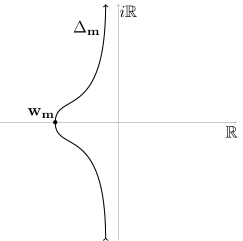
Figure 4: The contour $\Delta_{m}.$

Recall that if $\Gamma$ is a steepest descent contour through the unique saddle point of a degree two polynomial $p(z)=-\alpha z^{2}+\beta z,$ then we have the following exact formula known as Gaussian integration

$$\int_{\Gamma}\exp(p(z))\ \operatorname{{d}\hskip-1.70717pt}z=\sqrt{\frac{\pi}{\alpha}}\exp\left(\frac{\beta^{2}}{4\alpha}\right).$$

Applying Gaussian integration to the polymonials $p_{m}$ gives us the following identity

$$(-1)^{n}\Psi(q)=\sum_{m=m_{0}}^{\infty}c_{m}q^{\frac{m^{2}}{4P}}=\sum_{m=m_{0}}^{\infty}c_{m}\frac{1}{\sqrt{\pi h}}\int_{i\mathbb{R}}\exp\left(p_{m}(w)\right)\operatorname{{d}\hskip-1.70717pt}w.$$ (117)

Choose a small postive parameter $\delta>0$ and introduce the contour

$$\Delta_{0}=e^{i\delta}i\mathbb{R}_{+}\cup e^{-i\delta}i\mathbb{R}_{-}\subset\{z\in\mathbb{C}:\operatorname{Re}(z)<0\}.$$

Let $\Upsilon\subset\{z\in\mathbb{C}:\Re(z)<0\}$ be the Hankel contour which encloses $\mathbb{R}_{-}$ and satisfies $\sqrt{\Upsilon}=\Delta_{0}.$ The orientation of these contours are given as in Figure 5.

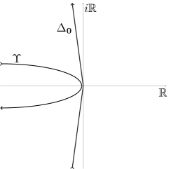
Figure 5: The contours $\Upsilon$ and $\Delta_{0}.$

We let

$$\Upsilon_{\pm}=\Upsilon\cap\{z\in\mathbb{C}:\operatorname{Im}(z)\in\mathbb{R}_{\mp}\},$$

so that $\sqrt{\Upsilon_{+}}=e^{i\delta}i\mathbb{R}_{+}$ and $-\sqrt{\Upsilon_{-}}=e^{-i\delta}i\mathbb{R}_{-}$ where $\sqrt{\cdot}$ denotes the principal branch of the square root. Introduce the variable

$$w^{2}=v.$$

As $\Delta_{0}$ is a small deformation of $\Delta_{m}$ for each $m\in\mathbb{Z}_{\geq m_{0}},$ we obtain

$$\begin{split}\sum_{m=m_{0}}^{\infty}\frac{c_{m}}{\sqrt{\pi h}}\int_{i\mathbb{R}}\exp(p_{m}(w))\ \operatorname{{d}\hskip-1.70717pt}w&=\sum_{m=m_{0}}^{\infty}\sum_{\epsilon=\pm 1}\frac{c_{m}}{\sqrt{\pi h}}\ \int_{\Upsilon(\epsilon)}\frac{\exp\left(-\frac{v}{h}+\epsilon\frac{m}{\sqrt{P}}\sqrt{v}\right)}{\epsilon 2\sqrt{v}}\ \operatorname{{d}\hskip-1.70717pt}v\\ &=\sum_{\epsilon=\pm 1}\frac{1}{2\sqrt{\pi h}}\int_{\epsilon\Upsilon(\epsilon)}\frac{\exp(-\frac{v}{h})}{\sqrt{v}}\sum_{m=m_{0}}^{\infty}c_{m}e^{\epsilon\frac{m\sqrt{v}}{\sqrt{P}}}\ \operatorname{{d}\hskip-1.70717pt}v\\ &=\sum_{\epsilon=\pm 1}\frac{1}{2\sqrt{\pi h}}\int_{\epsilon\Upsilon(\epsilon)}\exp\left(-\frac{v}{h}\right)\mathcal{B}(v)\ \operatorname{{d}\hskip-1.70717pt}v\end{split}$$ (118)

In the second equality of (118) we used that $\epsilon\sqrt{v}\in\{z\in\mathbb{C}:\operatorname{Re}{z}<0\}$ for all $v\in\Upsilon(\epsilon),$ and the contour $-\Upsilon(-1)$ denotes $\Upsilon(-1)$ but oriented in the direction from the origin and towards infinity. In the third equality of (118) we used equation (116) and the identity

$$G(z)=G\left(\frac{1}{z}\right),$$ (119)

which follows directly from the definition of $G$. Now introduce the variable

$$\xi=\frac{v}{2\pi i}.$$

This identifies (up to a small deformation) the $v$ contour $\Upsilon_{+}-\Upsilon_{-}$ with the $\xi$ contour $\varGamma$ introduced in Figure 1.

We have

$$\sum_{\epsilon=\pm 1}\frac{1}{2\sqrt{\pi h}}\int_{\epsilon\Upsilon(\epsilon)}\exp\left(-\frac{v}{h}\right)\mathcal{B}(v)\ \operatorname{{d}\hskip-1.70717pt}v\\ =\sum_{\epsilon=\pm 1}\frac{2\pi i}{2\sqrt{\pi h}}\int_{\exp(\epsilon\frac{\pi i}{4})i\mathbb{R}_{+}}\exp\left(-\frac{2\pi i\xi}{h}\right)\mathcal{B}(2\pi i\xi)\ \operatorname{{d}\hskip-1.70717pt}\xi\\ =\sum_{\epsilon=\pm 1}\frac{2\pi i}{2\sqrt{\pi h}}\frac{\sqrt{2\pi i}}{8\kappa}\int_{\exp(\epsilon\frac{\pi i}{4})i\mathbb{R}_{+}}\exp\left(-\frac{2\pi i\xi}{h}\right)\mathcal{B}(\operatorname{Z}_{0})(\xi)\ \operatorname{{d}\hskip-1.70717pt}\xi.$$ (120)

In the last equality of (120) we used Equation (115), which relates $\mathcal{B}$ and $\mathcal{B}(\operatorname{Z}_{0}).$ Now recall that $\kappa=\sqrt{2\pi iP}$, since $H=1$ and recognize the pre-factor in the last line of (120) as

$$\frac{2\pi i}{2\sqrt{\pi h}}\frac{1}{\sqrt{P}2}=(-1)^{n}\frac{\lambda}{\sqrt{\tau}},$$ (121)

where $\lambda$ is the scalar introduced in the statement of Theorem 3. By combining Equations (117), (118) and (120), we see that Equation (114) holds.

Write $\hat{\operatorname{Z}}_{0}(X;q)=\hat{\operatorname{Z}}_{0}(q)$. We now show that

$$\Psi(q)=q^{\Delta}\hat{\operatorname{Z}}_{0}(q),$$ (122)

where $\Delta\in\mathbb{Q}$ is the scalar introduced in (113). This will establish (12) and thereby finish the proof. We start with $\hat{\operatorname{Z}}_{0}(q).$ By Definition 1 and since in this case $\phi=0$, we have that

$$\hat{\operatorname{Z}}_{0}(q)=q^{\frac{3\sigma-\sum_{v}m_{v}}{4}}\sum_{\vec{l}\in 2M\mathbb{Z}^{s}}q^{-\frac{(\vec{l},M^{-1}\vec{(}l))}{4}}\oint_{\lvert z_{v}\rvert=1}\prod_{v\in V}\frac{\operatorname{{d}\hskip-1.70717pt}z_{v}}{2\pi iz_{v}}\left(z_{v}-\frac{1}{z_{v}}\right)^{2-\text{deg}(v)}z_{v}^{l_{v}}.$$ (123)

Here it is understood that we have taken the principal value of the integral as explained above. Recall that for a Laurent series $a(z)=\sum_{j\in\mathbb{Z}}a_{j}z^{j}$ we have that

$$v.p.\oint_{\lvert z\rvert=1}\frac{\operatorname{{d}\hskip-1.70717pt}z}{2\pi iz}a(z)=a_{0}.$$

For our star-shaped plumbing graph $\Gamma,$ the non-zero contributions to (123) comes from $\vec{l}\in 2M\mathbb{Z}^{s}$ with $l_{w}=0$ for all of the entries corresponding to an internal vertex $w$ of an arm, and $l_{v}=\pm 1$ if $v$ is a terminal vertex of an arm and then from the central vertex $v_{0}$, which we will now consider.

In comparing $\hat{\operatorname{Z}}_{0}(q)$ with $\Psi(q)$ it is useful to introduce the integer sequence $\{a_{j}\}_{j=0}^{\infty}$ determined by

$$\left(t-t^{-1}\right)^{2-n}=\begin{cases}\sum_{j=0}^{\infty}a_{j}t^{2j+n-2},\ &\text{if}\ \lvert t\rvert<1\\ \\ \sum_{j=0}^{\infty}(-1)^{n}a_{j}t^{-2j-n+2},\ &\text{if}\ \lvert t\rvert>1.\end{cases}$$ (124)

The $a_{j}$’s can be explicitly evaulated: By the formula for the geometric series $(1-t)^{-1}=\sum_{j=0}^{\infty}t^{j}$ and Cauchy multiplication of power series, we see that

$$\frac{1}{(1-t)^{m}}=\sum_{j=0}^{\infty}\left(\sum_{j_{1}+\cdots+j_{m}=j}1\right)t^{j}=\sum_{j=0}^{\infty}{{j+m-1}\choose{j}}t^{j},$$

and therefore one sees that

$$a_{j}=(-1)^{n}{{j+n-3}\choose{j}}.$$

However for the comparison of $\hat{\operatorname{Z}}_{0}(q)$ and $\Psi(q)$ given below, we don’t need the closed form for $a_{j}$, but rather the equation (124).

Write $z_{v_{0}}=z$ and $l=l_{v_{0}}$. We obtain

$$v.p.\oint_{\lvert z\rvert=1}\frac{\operatorname{{d}\hskip-1.70717pt}z}{2\pi iz}\left(z-z^{-1}\right)^{2-n}z^{l}=\begin{cases}\frac{1}{2}a_{\frac{l-n+2}{2}}\ &\text{if}\ 2-n-l\in 2{\mathbb{Z}}_{+},\\ \\ \frac{1}{2}(-1)^{n}a_{\frac{2-n-l}{2}}&\ \text{if}\ l-n+2\in 2{\mathbb{Z}}_{+},\\ \\ a_{0}\ &\text{if}\ l=0,n=2.\par\end{cases}$$ (125)

We know that the adjacency matrix $M$ is unimodular, and so $M\mathbb{Z}^{s}=\mathbb{Z}^{s}.$ Define a map $\vec{l}:\{\pm 1\}\times\mathbb{N}\times\{\pm 1\}^{n}\rightarrow\mathbb{Z}^{s}$ as follows: For the central vertex $v_{0}$ we have

$$\vec{l}(\varepsilon,j,\epsilon)_{v_{0}}=\varepsilon(-2j+2-n).$$ (126)

For $m=1,...,n$ and the terminal vertex $v$ of the $m^{\prime}$th arm, we have

$$\vec{l}(\varepsilon,j,\epsilon)_{v}=\epsilon_{m},$$

and for every internal vertex $w$ of the arms, we have

$$\vec{l}(\varepsilon,j,\epsilon)_{w}=0.$$

With this notation, the above considerations show that

$$\hat{\operatorname{Z}}_{0}(q)=q^{-\frac{3s+\sum_{v}m_{v}}{4}}\sum_{\varepsilon=\pm 1}\sum_{r=0}^{\infty}\sum_{\epsilon\in\{\pm 1\}^{n}}(-1)^{\frac{(1-\varepsilon)(n-2)}{2}}\frac{a_{r}}{2}\left(\prod_{j=1}^{n}\epsilon_{j}\right)q^{-\frac{\left\langle\vec{l}(\varepsilon,r,\epsilon),M^{-1}\vec{l}(\varepsilon,r,\epsilon),\right\rangle}{4}}.$$ (127)

If we apply the symmetry that simultaneously changes the sign of all $\epsilon_{j}$ and $\varepsilon,$ then we we obtain

$$\hat{\operatorname{Z}}_{0}(q)=(-1)^{n}q^{-\frac{3s+\sum_{v}m_{v}}{4}}\sum_{r=0}^{\infty}\sum_{\epsilon\in\{\pm 1\}^{n}}a_{r}\left(\prod_{j=1}^{n}\epsilon_{j}\right)q^{-\frac{\left\langle\vec{l}(-1,r,\epsilon),M^{-1}\vec{l}(-1,r,\epsilon),\right\rangle}{4}}.$$ (128)

The quadratic form

$$\vec{l}\mapsto\langle\vec{l},M^{-1}\vec{l}\rangle/4$$

was computed for $n=3$ in [28] in their proof of Proposition $4.8$. The size of the matrix $M^{-1}$ is irrevelant to their computation, and their formula can be generalized to our case to give the formula

$$\hat{\operatorname{Z}}_{0}(q)=(-1)^{n}q^{-\Delta}\sum_{r=0}^{\infty}\sum_{\epsilon\in\{\pm 1\}^{n}}a_{r}\left(\prod_{j=1}^{n}\epsilon_{j}\right)q^{\frac{P}{4}\left(2r+(n-2)+\sum_{j=1}^{n}\epsilon_{j}\frac{1}{p_{j}}\right)^{2}.}$$ (129)

We now compute $\Psi(q).$ For $\lvert z\rvert<1$ we have

$$G(z)= \prod_{j=1}^{n-2}\left(z^{\frac{P}{p_{j}}}-z^{-\frac{P}{p_{j}}}\right)\left(z^{P}-z^{-P}\right)^{2-n}$$ (130)

$$= \sum_{r=0}^{\infty}\sum_{\epsilon\in\{\pm 1\}^{n}}a_{r}\left(\prod_{j=1}^{n}\epsilon_{j}\right)z^{2Pr+P(n-2)+\sum_{j=1}^{n}\epsilon_{j}\frac{P}{p_{j}}}.$$ (131)

It follows that

$$\Psi(q)=(-1)^{n}\sum_{r=0}^{\infty}\sum_{\epsilon\in\{\pm 1\}^{n}}a_{r}\left(\prod_{j=1}^{n}\epsilon_{j}\right)q^{\frac{\left(2Pr+P(n-2)+\sum_{j=1}^{n}\epsilon_{j}\frac{P}{p_{j}}\right)^{2}}{4P}}.$$ (132)

This shows (122). ∎

We obtain the following corollary.

Corollary 12.

Let $\operatorname{Z}_{0}\in x^{-1/2}\mathbb{C}[[x^{-1}]]$ be the normalization of the Ohtsuki series from Theorem 2. We have an asymptotic expansion

$$q^{\Delta}\hat{\operatorname{Z}}_{0}(X;q)\sim_{q\rightarrow 1}\frac{2\lambda}{\sqrt{\tau}}\operatorname{Z}_{0}(1/\tau).$$ (133)

Proof.

This is a consequence of the integral formula (12) from Theorem 3

$$q^{\Delta}\hat{\operatorname{Z}}_{0}(X;q) =\frac{\lambda}{\sqrt{\tau}}\int_{\varGamma}\exp(-\zeta/\tau)\mathcal{B}(\operatorname{Z}_{0})(\zeta)\ \operatorname{{d}\hskip-1.70717pt}\zeta$$ (134)

$$=\frac{\lambda}{\sqrt{\tau}}\sum_{\epsilon\in\{\pm 1\}}\mathcal{L}_{\varGamma_{\epsilon}}(\mathcal{B}(\operatorname{Z}_{0}))(1/\tau)$$ (135)

and Borel-Laplace resummation, which is stated as Theorem 15 below. ∎

Let us now recall previous work on the $q$-series $\Psi.$ We start with the case $n=3,$ for which more is known. As already mentioned in the introduction, Lawrence and Zagier have shown in [40] that the quantum invariant $\tau_{k}(X)$ can be recovered as the radial limit of $\Psi(q),$ as $q$ tends to $\exp(2\pi i/k)$. This was generalized to $n=4$ by Hikami in [34] but with corrections terms appearing. The series $\Psi$ have interesting arithmetic properties; the coefficients $\chi(m)$ are periodic functions of period $2P$ and $\Psi$ is the so-called Eichler integral of a mock modular form with weight $3/2.$ As mentioned in the introduction the connection between quantum invariants and number theory was further pursued by Hikami in a number of articles [30, 32, 34, 35, 36]. For general $n\geq 3$ we mention again the work [25] of Fuji, Iwaki, Murakami and Terashima which was discussed in the introduction.

Let us now discuss what was previosly known about the $q$-series invariant $\hat{\operatorname{Z}}_{0}(X).$ In [28] it was shown that when $X$ is a Briskekorn sphere $\Sigma(p_{1},p_{2},p_{3}),$ (i.e. $n=3$) then $\hat{\operatorname{Z}}_{0}(X)$ is a linear combination of so-called false theta functions. The $q$-series invariant $\hat{\operatorname{Z}}_{0}$ was also considered for certain Seifert fibered manifolds (with up to $n=4$ singular fibers) in the work [14], as well as a proposed analog of $\hat{\operatorname{Z}}_{0}$ for higher rank gauge group - see also [47] for further developments in this direction. In this paper we work exclusively with $G=\operatorname{SU}(2)$).

In connection with the work [40], Zagier invented the notion of a quantum modular form. This notion was generalized by Bringmann et al. in [8], where they introduce the notion of a higher depth quantum modular form. For any $n\geq 3,$ it is known, that $\Psi$ is a linear combination of derivatives of quantum modular forms [9, 10]. It is interesting to observe that $\Psi$ is obtained from the Borel transform through a resummation process reminiscent of the median resummation of [15]. Moreover as explained in [12] it is expected that for a general $3$-manifold $M,$ Mock/false modular form duality is related to $\widehat{Z}_{a}(M;q)$, i.e. there exists an associated pair of a so-called Mock modular form and a so-called false modular form, and these are related by a $q\mapsto q^{-1}$ transformation and have the same transseries expression near $q\rightarrow 1.$ This is quite possibly connected to the conjecture $2$ in [26] (called the symmetry conjecture). Let us also mention the work [18] by Dimofte-Garoufalidis which connects modularity in quantum topology with complex Chern-Simons theory.

4 The asymptotic expansion of the GPPV invariant

The invention of $\hat{\operatorname{Z}}$ was party motivated by an attempt to generalize the following discovery of Lawrence and Zagier. Set $q_{k}=\exp(2\pi i/k).$ For $n=3$ they proved in [40] the identity (for some $\sigma\in\mathbb{Q})$

$$\tau_{k}\left(\Sigma(p_{1},p_{2},p_{3})\right)(q_{k}-1)q_{k}^{\sigma}=-\frac{1}{2}\lim_{q\rightarrow q_{k}}\sum_{m=m_{0}}^{\infty}\chi_{m}q^{\frac{m^{2}}{4P}}.$$

For a closed oriented $3$-manifold $Y$ consider the normalized WRT invariant

$$\operatorname{Z}_{\operatorname{CS}}(Y;k)=\frac{\tau_{k}(Y)}{\tau_{k}(\operatorname{S}^{2}\times\operatorname{S}^{1})}.$$ (136)

We now state the radial limit conjecture.

Conjecture 2 ([28]).

Let $Y$ be a closed oriented $3$-manifold with $b_{1}(Y)=0.$ Set

$$T=\operatorname{Spin^{c}}(Y)/\mathbb{Z}_{2}.$$

For every $a\in T,$ there exists invariants

$$\Delta_{a}\in\mathbb{Q},\ c\in\mathbb{Z}_{+},\ \hat{\operatorname{Z}}_{a}(q)\in 2^{-c}q^{\Delta_{a}}\mathbb{Z}[[q]],$$

with the following properties. The series $\hat{\operatorname{Z}}_{a}(q)$ is convergent inside the unit disc $\{q\mid\ \lvert q\rvert<1\},$ and for infinitely many $k\in\mathbb{N}$ the radial limits $\lim_{q\uparrow\exp(2\pi i/k)}\hat{\operatorname{Z}}_{a}(q)$ exists and we have that

$$\operatorname{Z}_{\operatorname{CS}}(Y;k)=(i\sqrt{2k})^{-1}\sum_{a,b\in T}e^{2\pi iklk(a,a)}\lvert\mathcal{W}_{b}\rvert^{-1}S_{a,b}\lim_{q\uparrow\exp(2\pi i/k)}\hat{\operatorname{Z}}_{b}(q).$$ (137)

Here

$$S_{a,b}=\frac{e^{2\pi ikl(a,b)}+e^{-2\pi ikl(a,b)}}{\lvert\mathcal{W}_{a}\rvert\sqrt{\lvert\operatorname{H}_{1}(Y;Z)\rvert}},$$

and $\mathcal{W}_{x}$ is the $\mathbb{Z}_{2}$-stabilizer of $x.$

Remark 3.

Conjecture 2 appeared in slighly different form in [12, 29, 27].

The level $k$ WRT invariant $\tau_{k}(M)$ of a closed oriented $3$-manifold $M$ can be seen as a function of the $k$-root of unity $q_{k}=\exp(2\pi i/k)$, and as such it is a function of a certain subset of the boundary of the unit disc $\operatorname{D}=\{q:\lvert q\rvert<1\}.$ Assume $b_{1}(M)=0$ and define the $k$-dependent $q$-series

$$\hat{\operatorname{Z}}_{k}(M;q)=(i\sqrt{2k})^{-1}\sum_{a,b\in T}e^{2\pi ik\ lk(a,a)}\lvert\mathcal{W}_{b}\rvert^{-1}S_{a,b}\hat{\operatorname{Z}}_{b}(q).$$ (138)

Then $\hat{\operatorname{Z}}_{k}(M;q)$ is convergent for $q\in\operatorname{D}$ and the radial limit conjecture states

$$\lim_{q\uparrow q_{k}}\hat{\operatorname{Z}}_{k}(M;q)=\tau_{k}(M).$$

Thus $\hat{\operatorname{Z}}_{k}(M;q)$ can be seen as an analytic extension of $\tau_{k}(M)$ to the interior of the unit disc as illustrated in Figure 6 below

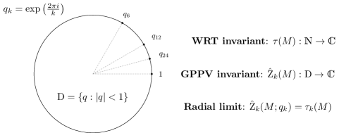
Figure 6: Analytic extension of $\tau_{k}(M)$.

4.1 Proof of Theorem 4

To simplify notation, we write

$$\hat{\operatorname{Z}}_{0}(X;q)=\hat{\operatorname{Z}}(q).$$

Recall the decomposition (27) of the normalized quantum invariant $\tilde{\operatorname{Z}}_{k}(X)$ into an integral part $\operatorname{Z}^{\operatorname{I}}$ and a residue part $\operatorname{Z}^{R}$. In Lemma 1 we prove the existence of an analogous decomposition for $\hat{\operatorname{Z}}_{0}(q)$ into a Laplace integral part $\mathcal{L}$ and a residue part $R$

$$q^{\Delta}\hat{\operatorname{Z}}_{0}(q)=\mathcal{L}(\tau)+R(\tau),$$ (139)

where we recall that $q=e^{2\pi i\tau}.$ We present in Proposition 13 a standard result in complex analysis [40] which asserts that a $q$-series with periodic coefficients of mean value zero has an asymptotic expansion, as $q$ tends to a root of unity. We then show in Proposition 14 that $R$ satisfy this hypothesis. Finally, we apply Proposition 13 to prove Theorem 4.

4.1.1 The decomposition of the GPPV invariant

Recall that $q=\exp(2\pi i\tau)$ with $\tau\in\mathfrak{h}$ where $\mathfrak{h}$ denotes the upper half plane, and recall the definitions of $F\in\mathcal{M}(\mathbb{C})$ and $g\in\mathbb{C}[x]$ given in (24). Let $\tilde{\Gamma}_{+}=e^{\frac{\pi i}{4}}$.

Lemma 1.

Introduce the holomorphic functions $\mathcal{L},R\in\mathcal{O}(\mathfrak{h})$ given by

$$\mathcal{L}(\tau) =\frac{2\lambda}{\sqrt{\tau}}\int_{\varGamma_{+}}e^{-x/\tau}\mathcal{B}(\operatorname{Z}_{0})(x)\ \operatorname{{d}\hskip-1.70717pt}x,$$ (140)

$$R(\tau) =-\frac{2\lambda}{\sqrt{\tau}}\sum_{m=0}^{\infty}\operatorname{Res}\left(\exp\left(\frac{g(\xi)}{\tau}\right)F(\xi),\xi=2\pi im\right).$$ (141)

Then we have that

$$q^{\Delta}\hat{\operatorname{Z}}_{0}(q)=\mathcal{L}(\tau)+R(\tau).$$ (142)

For $\tau$ in the first quadrant $\mathfrak{h}_{+}=\{z\in\mathfrak{h}\mid\Re(z)>0\}$ we have that

$$\mathcal{L}(\tau)=\frac{2\lambda}{\sqrt{\tau}}\int_{0}^{\infty}e^{-x/\tau}\mathcal{B}(\operatorname{Z}_{0})(x)\ \operatorname{{d}\hskip-1.70717pt}x.$$ (143)

Proof of Lemma 1.

Recall the contour formula from Theorem 3

$$q^{\Delta}\hat{\operatorname{Z}}_{0}(q)=\operatorname{I}(\tau)=\frac{\lambda}{\sqrt{\tau}}\int_{\varGamma}\exp(-x/\tau)\mathcal{B}(\operatorname{Z}_{0})(x)\ \operatorname{{d}\hskip-1.70717pt}x.$$ (144)

Under the coordinate change

$$x=y^{2}$$ (145)

the contour $\varGamma$ corresponds to the contour

$$\varPsi=e^{i\pi\frac{3}{8}}\mathbb{R}_{+}+e^{i\pi\frac{1}{8}}\mathbb{R}_{+}$$ (146)

Therefore we have that

$$q^{\Delta}\hat{\operatorname{Z}}_{0}(q)=\frac{\lambda}{\sqrt{\tau}}\int_{\varPsi}\exp(-y^{2}/\tau)\mathcal{B}(\operatorname{Z}_{0})(y^{2})2y\ \operatorname{{d}\hskip-1.70717pt}y.$$ (147)

Introduce the meromorphic function $B\in\mathcal{M}(\mathbb{C})$ given for all $y\in\mathbb{C}$ by

$$B(y)=2y\mathcal{B}(\operatorname{Z}_{0})(y^{2}).$$ (148)

By Theorem 2 we have that

$$B(y)=\frac{2\kappa}{\pi i}G\left(\exp\left(\frac{\kappa y}{P}\right)\right)=\frac{2\kappa}{\pi i}F\left(\frac{\kappa y}{2}\right).$$ (149)

From (149) we see that $B$ is periodic with period $\kappa$, i.e. for all $m\in\mathbb{Z}$ we have that

$$B(y+\kappa m)=B(y).$$ (150)

Let $\mathcal{P}$ be the set of poles of $B$. It follows from Theorem 2 that $\mathcal{P}$ is a subset of the axis $e^{\pi i/4}\mathbb{R}$ and that

$$\{-\omega^{2}\mid\omega\in\mathcal{P}\}=2\pi i\operatorname{CS}_{\mathbb{C}}(X)+2\pi i\mathbb{Z}.$$ (151)

Write

$$\varPsi_{\pm}=e^{i\pi(\frac{1}{4}\mp\frac{1}{8})}\mathbb{R}_{+}.$$

We will now apply Cauchy’s residue theorem to move $\varPsi_{-}$ across $e^{i\pi/4}\mathbb{R}_{+}$ to $\varPsi_{+}$ in order to obtain the formula (142). Deform $\varPsi_{\pm}$ on the complement of a neighbourhood around the origin to two curves $L_{\pm}$, which are parallel to $e^{i\pi/4}\mathbb{R}_{+}$ outside this neighbourhood of the origin, as indicated in Figure 7. Set

$$L=L_{+}\cup L_{-}.$$

We first show that

$$\int_{\varPsi}\exp(-y^{2}/\tau)B(y)\ \operatorname{{d}\hskip-1.70717pt}y=\int_{L}\exp(-y^{2}/\tau)B(y)\ \operatorname{{d}\hskip-1.70717pt}y,$$ (152)

and then we show that the right hand side of (152) can be rewritten as a sum of residues. Let $R>0$ be a positive constant, and let $R_{\pm}$ be the arc segment of the circle of radius $R$, which connects $\varPsi_{\pm}$ and $L_{\pm}$. Because $L_{\pm}$ is parallel to $\kappa\mathbb{R}_{+}$ outside a neighbourhood of the origin, there exists a real positive constant $b_{0}>0$ such that every $y\in R_{\pm}$ is of the form

$$y=\kappa a\pm b,(a,b)\in\mathbb{R}_{+}\times[b_{0},+\infty)$$

and therefore exists a positive real constant $A>0$ independent of $R$, which gives an upper bound

$$\left\lvert\frac{1}{1-e^{-\kappa y}}\right\rvert<\frac{1}{1-\exp\left(-\Re(\kappa)b_{0}\right)}:=A>0$$ (153)

for all $y\in R_{+}$. It follows that we obtain a uniform estimate

$$\begin{split}B(y)&=2^{n-2}\frac{2\kappa}{\pi i}\frac{\prod_{j=1}^{n}\sinh(\frac{\kappa y}{2p_{j}})}{\left(e^{\kappa y/2}(1-e^{-y\kappa})\right)^{n-2}}\\ &=O\left(e^{-y\kappa/2}\prod_{j=1}^{n}\sinh\left(\frac{\kappa y}{2p_{j}}\right)\right)=O(e^{A_{1}R}).\end{split}$$ (154)

for all $y\in R_{+}$ for a real constant $A_{1}$. For fixed $\tau$, there exists a positive real constant $A_{2}>0$ giving a uniform bound on $R_{+}$

$$e^{-y^{2}/\tau}=O(e^{-A_{2}R^{2}}).$$ (155)

By combining the estimates (154) and (155), and using that the arc length of $R_{\pm}$ is proportional to $R$, we obtain the estimate

$$\int_{R_{+}}\exp(-y^{2}/\tau)B(y)\ \operatorname{{d}\hskip-1.70717pt}y=O(Re^{-A_{2}R^{2}+A_{1}R}).$$ (156)

By similar reasoning, there exists constants $B_{2}>0,B_{1}\in\mathbb{R}$ giving the estimate

$$\int_{R_{-}}\exp(-y^{2}/\tau)B(y)\ \operatorname{{d}\hskip-1.70717pt}y=O(Re^{-B_{2}R^{2}+B_{1}R}).$$ (157)

Thus we obtain that

$$\lim_{R\rightarrow\infty}\sum_{\epsilon\in\{\pm 1\}}\int_{R_{\epsilon}}\exp(-y^{2}/\tau)B(y)\ \operatorname{{d}\hskip-1.70717pt}y=0,$$ (158)

which gives the desired identity (152) .

We now turn to the computation of $\int_{L}\exp(-y^{2}/\tau)B(y)\ \operatorname{{d}\hskip-1.70717pt}y$. For each $m\in\mathbb{N}$, let $L_{m}$ be a small line segment with

$$L_{m}\cap e^{i\pi/4}\mathbb{R}_{+}=\{m\kappa\},$$

and which meets $e^{i\pi/4}\mathbb{R}_{+}$ in a right angle. We can arrange that $L_{m}$ is of fixed lenght and that $L_{m}$ meet $L_{\pm}$ in a point. Thus we have

$$L_{m}=L_{0}+m\kappa$$ (159)

Let $L^{m}_{\pm}$ be the bounded component of $L_{\pm}\setminus L_{m},$ and let $\mathcal{P}_{m}\subset\mathcal{P}$ be the set of poles of $B$ that lie within the bounded component of the complement of the contour

$$\varPsi_{m}=L^{m}_{+}\cup L_{m}\cup L^{m}_{-}.$$

See Figure 7.

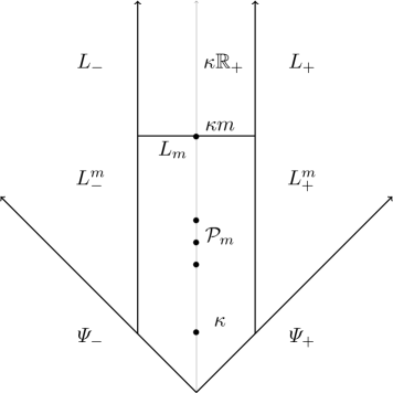
Figure 7: The contours $L_{\pm},L^{m}_{\pm}$ and $\varPsi_{\pm}$ and the subset of poles $\mathcal{P}_{m}$ drawn rotated, such that $\kappa\mathbb{R}_{+}$ points straight up.

Equip $\varPsi_{m}$ with the counter clockwise orientation. An application of Cauchy’s residue theorem now gives

$$\begin{split}2\pi i\sum_{\omega\in\mathcal{P}_{m}}\operatorname{Res}(e^{-y^{2}/\tau}B(y),y=\omega)=\int_{\varPsi_{m}}\exp(-y^{2}/\tau)B(y)\ \operatorname{{d}\hskip-1.70717pt}y\\ =\int_{L_{m}}\exp(-y^{2}/\tau)B(y)\ \operatorname{{d}\hskip-1.70717pt}y+\sum_{\epsilon\in\{\pm 1\}}\epsilon\int_{L^{m}_{\epsilon}}\exp(-y^{2}/\tau)B(y)\ \operatorname{{d}\hskip-1.70717pt}y.\end{split}$$ (160)

Because $B$ is $\kappa$ periodic as stated in (150) and $L_{m}=L_{0}+m\kappa$, we see that that there exists $C>0$ giving a uniform bound

$$C>\sup\{\lvert B(y)\rvert\ \mid\ y\in\cup_{m\in\mathbb{N}}L_{m}\}.$$ (161)

Because of this universal bound, it is easy too see that

$$\lim_{m\rightarrow\infty}\int_{L_{m}}\exp(-y^{2}/\tau)B(y)\ \operatorname{{d}\hskip-1.70717pt}y=0.$$ (162)

It follows that the right hand side of (160) converges to

$$\sum_{\epsilon\in\{\pm 1\}}\int_{L_{\epsilon}}\exp(-y^{2}/\tau)B(y)\ \operatorname{{d}\hskip-1.70717pt}y=\sum_{\epsilon\in\{\pm 1\}}\epsilon\int_{\varPsi_{\epsilon}}\exp(-y^{2}/\tau)B(y)\ \operatorname{{d}\hskip-1.70717pt}y.$$

This also implies that the sum of residues is convergent.

Let us now recall a simple transformation law for residues. Let $z_{0}\in\mathbb{C}$ and let $f\in\mathcal{M}_{z_{0}}(\mathbb{C})$ be the germ of a meromorphic function with a pole at $z_{0}.$ Assume $w_{0}\in\mathbb{C}$ and that $z\in\mathcal{O}_{w_{0}}(\mathbb{C})$ satisfies $z(w_{0})=z_{0},\dot{z}(w_{0})\not=0.$ If either $z_{0}$ is a simple pole, or $z(w)$ is linear in $w,$ then we have that

$$\text{Res}(f(z(w)),w=w_{0})=\frac{\text{Res}(f(z),z=z(w_{0}))}{\dot{z}(w_{0})}.$$ (163)

Introduce the variable

$$\xi=\frac{\kappa y}{2}.$$ (164)

By using the relation (149) between $B$ and $F$, the relation (148) between $B$ and $\mathcal{B}(\operatorname{Z}_{0})$ and the tranformation law (163) we obtain

$$\begin{split}q^{\Delta}\hat{\operatorname{Z}}_{0}(q)&=\frac{\lambda}{\tau}\int_{\varPsi}\exp\left(-\frac{y^{2}}{\tau}\right)B(y)\ \operatorname{{d}\hskip-1.70717pt}y\\ &=\frac{2\lambda}{\tau}\left(\int_{\varPsi_{+}}\exp\left(-\frac{y^{2}}{\tau}\right)B(y)\ \operatorname{{d}\hskip-1.70717pt}y-2\pi i\sum_{\omega\in\mathcal{P}}\operatorname{Res}(e^{-y^{2}/\tau}B(y),y=\omega)\right)\\ &=\frac{2\lambda}{\tau}\left(\int_{\Gamma_{+}}\exp\left(-\frac{x}{\tau}\right)\mathcal{B}(\operatorname{Z}_{0})(x)\ \operatorname{{d}\hskip-1.70717pt}x-\sum_{m=1}^{\infty}\operatorname{Res}(e^{-g(\xi)/\tau}F(\xi),\xi=2\pi im)\right)\\ &=\mathcal{L}(\tau)+R(\tau).\end{split}$$ (165)

Finally, we prove (143) for $\tau\in\mathfrak{h}_{+}$. First observe that for $x$ and $\tau$ in the upper right half plane we have

$$\Re(x/\tau)>0.$$ (166)

Push the contour $\tilde{\Gamma}_{+}$ to $\mathbb{R}_{+}$. If the integral is invariant under this deformation of the contour, we obtain the desired identity. To see that the integral is invariant under this deformation of the contour, we apply a limiting argument, together with Cauchy’s residue formula. To that end, let $R>0$ be a positive parameter, and let $C_{R}$ be the arc segment of the circle of radius $R$, which connects $R$ to $Re^{i\pi\frac{3}{4}}$ and stays in the upper half plane. As we are not moving the contour across any singularities of $\mathcal{B}(\operatorname{Z}_{0}),$ the only difficulty is to show that

$$\lim_{R\rightarrow+\infty}\int_{C_{R}}e^{-x/\tau}\mathcal{B}(\operatorname{Z}_{0})(x)\ \operatorname{{d}\hskip-1.70717pt}x=0.$$ (167)

As $C_{R}$ remain at least a fixed distance away from the axis of poles of $\mathcal{B}(\operatorname{Z}_{0})(x)$, the limit (167) follows by (166) together with arguments similar to the arguments giving the limit (158) above. ∎

4.1.2 Asymptotic expansions of $q$-series with periodic coefficients

Let $B_{m}(x)$ denote the $m$-th Bernoulli polynomial, i.e.

$$\frac{te^{tx}}{e^{t}-1}=\sum_{m=0}^{\infty}\frac{B_{m}(x)}{m!}t^{m}.$$ (168)

We recall the following result.

Proposition 13 ([31, 40]).

Let $C:\mathbb{Z}\rightarrow\mathbb{C}$ be a periodic function with period $M$ and mean value equal to zero

$$\sum_{m=1}^{M}C(n)=0.$$ (169)

Consider the $L$-series $L(s,C)$, which for $\Re(s)>1$ is defined by

$$L(s,C)=\sum_{m=1}^{\infty}\frac{C(m)}{m^{s}}.$$ (170)

This $L$-series admits an analytic extension to all of $\mathbb{C}$ and for $r\in\mathbb{N}$

$$L(-r,C)=-\frac{M^{r}}{r+1}\sum_{m=1}^{M}C(m)B_{r+1}\left(\frac{m}{M}\right).$$ (171)

For any polynomial $Q$ of degree $d$

$$Q(x)=\sum_{u=0}^{d}q_{u}x^{u}\in\mathbb{C}[x]$$

the following asymptotic expansions hold for real and positive $t$

$$\sum_{m=1}^{\infty}e^{-tm^{2}}C(m)Q(m)\ \underset{t\rightarrow 0}{\sim}\sum_{u=0}^{d}\sum_{r=0}^{\infty}q_{u}L(-2r-u,C)\frac{(-t)^{r}}{r!}.$$ (172)

Proof.

The existence of the analytic extension of the $L$-series of $C$, as well as the explicit evaluation (171) are proven in [40].

In [31, 40] the following asymptotic expansions are proven

$$\begin{split}&\sum_{m=1}^{\infty}C(m)e^{-tm^{2}}\ \underset{t\rightarrow 0}{\sim}\ \sum_{r=0}^{\infty}L(-2r,C)\frac{(-t)^{r}}{r!},\\ &\sum_{m=1}^{\infty}mC(m)e^{-tm^{2}}\ \underset{t\rightarrow 0}{\sim}\ \sum_{r=0}^{\infty}L(-2r-1,C)\frac{(-t)^{r}}{r!}.\end{split}$$ (173)

We have

$$\sum_{m=1}^{\infty}e^{-tm^{2}}C(m)Q(m)=\sum_{j=0}^{\infty}\frac{\partial^{j}}{\partial(-t)^{j}}\sum_{m=0}^{\infty}(q_{2j+1}m+q_{2j})e^{-tm^{2}},$$ (174)

where it is understood that $q_{l}=0$ for $l>d$. The expansion (172) follows formally from differentiating the expansions given in (LABEL:eq:asymptotixexpansions). This differentiation is valid because Poincare asymptotic expansions of analytic functions which are valid on suitable sectors can be termwise differentiated. Clearly $t\mapsto\sum_{m\geq 0}C(m)Q(m)\exp(-tm^{2})$ is an analytic function of $t$ in a small tubular neighbourhood of $(0,1]$, and from the proof given in [40] it is clear that the asymptotic expansions (LABEL:eq:asymptotixexpansions) are valid on such a small sector. ∎

Recall the definition of the meromorphic function $F$ given in (24). Next we prove that the coefficients of the principal part of $F$ at poles are periodic functions with mean value equal to zero.

Proposition 14.

For $j=1,2,...,n-2$ define $f_{j}:\mathbb{Z}\rightarrow\mathbb{C}$ as the coeficients of the principal part of $F$ at $2\pi im$ for $m\in\mathbb{Z}$, e.g. for $y$ near $2\pi im$

$$F(y)=\sum_{j=1}^{n-2}f_{j}(m)(y-2\pi im)^{-j}+\rm{reg.}.$$ (175)

Then each $f_{j}$ is $2P$-periodic and if $P$ is even, then we have for each even $k\in\mathbb{Z}$

$$\sum_{m=1,...,2P}e^{kg(2\pi im)}f_{j}(m)=0.$$ (176)

Proof.

The periodicity of the functions $f_{j},j=1,...,n-3$ follow directly from the $4\pi iP$-periodicity of $F$.

We now prove (176) assuming $P$ is even - which is equivalent to exactly one the $p_{j}$ being even. Using the definition (24) of $F$ we obtain

$$F(y+2\pi iP) =\frac{1}{4}\sinh(y/2+\pi iP)^{2-n}\prod_{j=1}^{n}\sinh(y/p_{j}+\pi iP/p_{j})$$ (177)

$$=(-1)^{nP}(-1)^{\sum_{j=1}^{n}\frac{P}{p_{j}}}F(y)=-F(y).$$ (178)

This implies that for each $j=1,...,n-3$ and $m=1,...,P$ we have

$$f_{j}(m+P)=-f_{j}(m).$$ (179)

On the other hand we have for integral $m$

$$g(2\pi i(P+m)) =\frac{i(2\pi i(P+m))^{2}}{8\pi P}=\frac{-i\pi m^{2}}{2P}\mp i\pi mP-\frac{i\pi P}{2}$$ (180)

$$=g(2\pi i(P\mp m))\mod\pi i\mathbb{Z}.$$ (181)

It follows that for even $k$ we have a pairwise cancellation

$$\sum_{m=1}^{2P}e^{kg(2\pi im)}f_{j}(m)=\sum_{m=1}^{P}e^{kg(2\pi im)}f_{j}(m)+e^{kg(2\pi i(m+P))}f_{j}(m+P)$$ (182)

$$=\sum_{m=1}^{P}e^{kg(2\pi im)}f_{j}(m)-e^{kg(2\pi im)}f_{j}(m)=0.$$ (183)

This concludes the proof. ∎

4.1.3 The asymptotic expansion of the GPPV invariant

Recall the definition the functions $F$ and $g$ given in (24). Let $m\in\mathbb{N}$. For $y$ close to $2\pi im$ we use the notation of Propositon 14 and write

$$F(y)=\sum_{j=1}^{n-2}f_{j}(m)(y-2\pi im)^{-j}+\rm{reg.},$$

where each $f_{j}:\mathbb{Z}\rightarrow\mathbb{C}$ is $2P$-periodic. For each $l\in\mathbb{N}$ there exists a uniquely determined polynomial

$$P_{l}(x,y)\in Q[\pi i,x,y]$$ (184)

such that

$$\frac{1}{l!}\frac{\partial^{l}e^{g(y)/\tau}}{\partial y^{l}}(2\pi im)=e^{g(2\pi im)/\tau}P_{l}(\tau^{-1},m).$$ (185)

There exists uniquely determined complex coefficients $p_{l,u,v,}$ with

$$P_{l}(\tau^{-1},m)=\sum_{u,v}p_{l,u,v}\tau^{-u}m^{v}.$$ (186)

Recall that $B_{m}(x)$ denotes the $m$’th Bernoulli polynomial and is defined by (168). Define for each $\theta\in\operatorname{CS}_{\mathbb{C}}(X)$ the following polynomials with coefficients in power series

$$\begin{split}R_{\theta}(k,t)&=\sum_{\begin{subarray}{c}m=1,...,2P,\\ g(2\pi im)\equiv 2\pi i\theta\end{subarray}}\sum_{j,u,v}f_{j}(m)k^{u}p_{j-1,u,v}\sum_{r=0}^{\infty}\frac{(2P)^{2r+v}}{2r+v+1}B_{2r+v+1}\left(\frac{m}{2P}\right)\frac{(-t)^{r}}{r!},\\ \check{\operatorname{Z}}_{\theta}(k,t)&=\sum_{\begin{subarray}{c}m=1,...,2P,\\ g(2\pi im)\equiv 2\pi i\theta\end{subarray}}\sum_{j,u,v}f_{j}(m)k^{u}p_{j-1,u,v}\sum_{r=1}^{\infty}\frac{(2P)^{2r+v}}{2r+v+1}B_{2r+v+1}\left(\frac{m}{2P}\right)\frac{(-t)^{r}}{r!}\end{split}$$ (187)

Observe

$$\check{\operatorname{Z}}_{\theta}(k,t)=R_{\theta}(k,t)-R_{\theta}(k,0),$$

i.e. $\check{\operatorname{Z}}_{\theta}$ is equal to $R_{\theta}$ minus the constant in the parameter $t$.

We can now prove Theorem 4.

Proof of Theorem 4.

Recall the decompsition

$$\frac{\sqrt{\tau}}{\lambda}q^{\Delta}\hat{\operatorname{Z}}=\mathcal{L}(\tau)+R(\tau)$$

given in Equation (142) in Lemma 1. Recall the decomposition of the normalized quantum invariant

$$\operatorname{Z}_{k}(X)=\operatorname{Z}^{\operatorname{I}}(k)+\operatorname{Z}^{R}(k)$$

given in (27). This decomposition together with equation (5), which relates the normalized quantum invariant $\tilde{\operatorname{Z}}_{k}(X)$ to the WRT invariant $\tau_{k}(X)$, shows the radial limit idenity can be proved by proving the following two limits.

$$\operatorname{Z}^{\operatorname{I}}(k)=\lim_{\tau\uparrow 1/k}\frac{\sqrt{\tau}}{2\lambda}\mathcal{L}(\tau), \operatorname{Z}^{R}(k)=\lim_{\tau\uparrow 1/k},\frac{\sqrt{\tau}}{2\lambda}R(\tau).$$ (188)

Observe that as $X$ is an integral homology sphere, the only $\operatorname{Spin^{c}}$ structure is $a=0$, and therefore the radial limit conjecture reduces (up to a scalar factor) to equation (16). We first focus on the integral part $\mathcal{L}(\tau)$. For every $k\in\mathbb{N}^{*}$ the integral part $\mathcal{L}(\tau)$ extends continuosly to $\tau=1/k$ and it follows from Equations (27), (92) and (143) that

$$(2\lambda\sqrt{k})^{-1}\mathcal{L}(1/k)=\mathcal{L}_{\mathbb{R}_{+}}(\mathcal{B}(\operatorname{Z}_{0}))(k)=\operatorname{Z}^{\operatorname{I}}(k).$$ (189)

Now recalling that $\tau_{k,t}=(k-i\frac{2Pt}{\pi})^{-1}$, we see that the non-trivial parts left in order to prove the asymptotic expansion (15) stated in Theorem 4 are the asymptotic expansion

$$\frac{\sqrt{\tau_{k,t}}}{2\lambda}R(\tau_{k,t})\ \underset{t\rightarrow 0}{\sim}\ \sum_{\theta\in\operatorname{CS}_{\mathbb{C}}(X)}e^{2\pi ik\theta}R_{\theta}(k,t),$$ (190)

and the identity

$$\sum_{\theta\in\operatorname{CS}_{\mathbb{C}}(X)}e^{2\pi ik\theta}R_{\theta}(k,0)=\operatorname{Z}^{R}(k).$$ (191)

We start with the expansion (190). To ease notation we set

$$g(2\pi im)=\theta_{m}.$$ (192)

We have

$$\operatorname{Res}(F(y)e^{g(y)/\tau},2\pi im)=e^{\theta_{m}/\tau}\sum_{j=1}^{n-3}f_{j}(m)P_{j-1}(\tau^{-1},m).$$ (193)

and accordingly

$$\frac{\sqrt{\tau}}{2\lambda}R(\tau)=-\sum_{m=0}^{\infty}e^{\theta_{m}/\tau}\sum_{j=1}^{n-3}f_{j}(m)P_{j-1}(\tau^{-1},m),$$ (194)

Note that $\tau_{k,t}\in\mathfrak{h}$ for $t\in(0,1)$. The function $g$ has the following transformation property

$$g(y+4\pi imP)=\frac{i(y+4\pi imP)^{2}}{8\pi P}=g(y)-my-2\pi im^{2}P.$$ (195)

Because of this, and the $2P$ periodicity of the $f_{j}$’s, we can write

$$\begin{split}\frac{\sqrt{\tau}}{2\lambda}R(\tau)=&-\sum_{m=0}^{\infty}e^{-tm^{2}}e^{kg(2\pi im)}\sum_{j=1}^{n-3}f_{j}(m)P_{j-1}(\tau^{-1},m)\\ =&-\sum_{j=1}^{n-2}\sum_{u,v}\sum_{m=0}^{\infty}e^{-tm^{2}}e^{k\theta_{m}}f_{j}(m)p_{j-1,u,v}\tau^{-u}m^{v}.\end{split}$$ (196)

Now for each $j,u=0,...,n-3$ we can apply Proposition 13 to the $2P$-periodic function of mean value zero given by

$$C_{j}(m)=e^{k\theta_{m}}f_{j}(m)$$ (197)

and the polynomial

$$Q_{j,u}(m)=\sum_{v}p_{j-1,u,v}m^{v}.$$ (198)

The fact that each $C_{j}$ is of mean value equal to zero follows from Proposition 14. The result of applying Proposition 13 is

$$\frac{\sqrt{\tau}}{2\lambda}R(\tau)\ \underset{t\rightarrow 0}{\sim}\ -\sum_{j,u,v}\sum_{r=0}^{\infty}k^{u}p_{j-1,u,v}L(-2r-v,C_{j})\frac{(-t)^{r}}{r!}$$ (199)

$$=\sum_{j,u,v}\sum_{r=0}^{\infty}k^{u}p_{j-1,u,v}\frac{(2P)^{2r+v}}{2r+v+1}\sum_{m=1}^{2P}C_{j}(m)B_{2r+v+1}\left(\frac{m}{2P}\right)\frac{(-t)^{r}}{r!}$$ (200)

$$=\sum_{m=1}^{2P}\sum_{j,u,v}e^{k\theta_{m}}f_{j}(m)k^{u}p_{j-1,u,v}\sum_{r=0}^{\infty}\frac{(2P)^{2r+v}}{2r+v+1}B_{2r+v+1}\left(\frac{m}{2P}\right)\frac{(-t)^{r}}{r!}.$$ (201)

This establishes the asymptotic expansion (190).

We now turn to the identity (191). Set

$$\begin{split}R_{0}(k)&=\sum_{\theta\in\operatorname{CS}_{\mathbb{C}}(X)}e^{2\pi ik\theta}R_{\theta}(k,0)=\sum_{m=1}^{2P}\sum_{j,u,v}e^{k\theta_{m}}f_{j}(m)p_{j-1,u,v}k^{u}\frac{(2P)^{v}}{v+1}B_{v+1}\left(\frac{m}{2P}\right).\end{split}$$ (202)

Let $x$ be a complex coordinate near $0$ and set $y_{m}=x+2\pi im$ for $m=1,2,...,2P$. Recall that

$$\operatorname{Z}^{R}(k)=-\sum_{m=1}^{2P-1}\operatorname{Res}\left(\frac{F(y)\exp\left(kg(y)\right)}{1-\exp(-ky)},y=2\pi im\right).$$ (203)

We have that

$$g(y_{m})=g(x+2\pi im)=\frac{i(x+2\pi im)^{2}}{8\pi P}=g(2\pi im)+g(x)-\frac{xm}{2P},$$ (204)

and accordingly

$$\exp(kg(y_{m}))=\exp\left(k\theta_{m}+kg(x)\right)\cdot\exp\left(-k\frac{xm}{2P}\right).$$ (205)

Recall that the polynomials $P_{l}$ defined in (185) as the coefficients of the Taylor series of $e^{kg(y)}$. Therefore it follows from Cauchy’s formula for multiplication of power series, the formula for the Taylor expansion of the exponential and the identity (205) that the following holds for all $k,m$

$$P_{c}(k,m)=\sum_{a+b=c}P_{a}(k,0)\left(\frac{-mk}{2P}\right)^{b}\frac{1}{b!}.$$ (206)

Writing this out in terms of coefficients gives

$$\sum_{c,u,v}p_{c,u,v}k^{u}m^{v} =\sum_{a+b=c}\sum_{s}p_{a,s,0}\left(\frac{(-1)}{2P}\right)^{b}\frac{1}{b!}k^{s+b}m^{b}.$$ (207)

This is equivalent to the identities

$$p_{j,u,0}\left(\frac{-1}{2P}\right)^{v}\frac{1}{v!}=p_{j+v,u+v,v}.$$ (208)

Recall the definition (168) of the Bernoulli polynomials $B_{m}$. Write

$$-\frac{F(y_{m})\exp\left(kg(y_{m})\right)}{1-\exp(-ky_{m})}=F(y_{m})\exp\left(k(g(x)+\theta_{m}\right)\frac{\exp\left(\frac{-kxm}{2P}\right)}{\exp(-kx)-1}=$$ (209)

$$\left(\sum_{j=1}^{n-3}f_{j}(m)x^{-j}+\rm{reg.}\right)\left(e^{k\theta_{m}}\sum^{\infty}_{a=0}P_{a}(k,0)x^{a}\right)\left(\sum_{b=0}^{\infty}\frac{B_{b}\left(\frac{m}{2P}\right)}{b!}(-kx)^{b-1}\right).$$ (210)

By comparing with Equation (202) and using the facts that $F$ has a multiple order zero at multiples of $4\pi iP$ and that we know that the $k^{-1}$ term cancels in $\operatorname{Z}^{R}(k)$, we obtain the desired identity

$$\operatorname{Z}^{R}(k)=\sum_{m=1}^{2P}\sum_{j=1}^{n-2}\sum_{\begin{subarray}{c}a+b=j,\\ a\geq 0,b\geq 1\end{subarray}}e^{k\theta_{m}}f_{j}(m)P_{a}(k,0)\frac{B_{b}\left(\frac{m}{2P}\right)}{b!}(-k)^{b-1}$$ (211)

$$=\sum_{m=1}^{2P}\sum_{j=1}^{n-2}\sum_{\begin{subarray}{c}a+b=j,\\ a\geq 0,b\geq 1\end{subarray}}e^{k\theta_{m}}f_{j}(m)P_{a}(k,0)\left(\frac{-1}{2P}\right)^{b-1}\frac{k^{b-1}}{(b-1)!}\frac{\left(2P\right)^{b-1}}{b}B_{b}\left(\frac{m}{2P}\right)$$ (212)

$$=\sum_{m=1}^{2P}\sum_{j=1}^{n-2}\sum_{\begin{subarray}{c}a+b=j,\\ a\geq 0,b\geq 1\end{subarray}}\sum_{s}e^{k\theta_{m}}f_{j}(m)p_{a,s,0}\left(\frac{-1}{2P}\right)^{b-1}\frac{k^{s+b-1}}{(b-1)!}\frac{\left(2P\right)^{b-1}}{b}B_{b}\left(\frac{m}{2P}\right)$$ (213)

$$\begin{split}&=\sum_{m=1}^{2P}\sum_{j=1}^{n-2}\sum_{\begin{subarray}{c}s,a+b=j,\\ a\geq 0,b\geq 1\end{subarray}}\sum_{s}e^{k\theta_{m}}f_{j}(m)p_{a+b-1,s+b-1,b-1}k^{s+b-1}\frac{(2P)^{b-1}}{b}B_{b}\left(\frac{m}{2P}\right)\end{split}$$ (214)

$$=\sum_{m=1}^{2P}\sum_{j=1}^{n-2}\sum_{u,v}e^{k\theta_{m}}f_{j}(m)p_{j-1,u,v}k^{u}\frac{(2P)^{v}}{v+1}B_{v+1}\left(\frac{m}{2P}\right)$$ (215)

$$=R_{0}(k).$$ (216)

In (LABEL:eq:UHAHAHA) we used the identity (208), and in (215) we set $u=s+b-1$ and $v=b-1$. This finishes the proof. ∎

Appendix A Resurgence and resummation

A.1 Resurgent functions and the Borel transform

The theory of resurgence was originally developed by Écalle in [21] and [22]. See [43] for an introduction to the mathematical theory of resurgence and see [20] for an introduction to the general use of resurgence in quantum field theory. Garoufalidis [26] and Witten [52] where the pioneers of the use of resurgence in quantum Chern-Simons theory.

Definition 2.

For a Riemann surface $C$ with universal covering space

$$\pi:\tilde{C}\rightarrow C$$

the algebra of resurgent functions is $\mathcal{R}(C)=\mathcal{M}(\tilde{C}).$

One source of resurgent functions are the Borel transforms of Laplace integrals. We now introduce the Borel transform. Let $\Gamma\in\mathcal{M}(\mathbb{C})$ be the Gamma function, which for $z\in\mathbb{C}$ with $\operatorname{Re}(z)>0$ is defined by

$$\Gamma(z)=\int_{0}^{\infty}e^{-t}t^{z-1}\operatorname{{d}\hskip-1.70717pt}t.$$ (217)

Definition 3.

Let $\{\alpha_{j}\}_{j=0}^{\infty}$ be an increasing sequence of positive real numbers, $\{\beta_{j}\}_{j=0}^{\infty}$ a sequence of non-negative integers and $\{c_{j}\}_{j=0}^{\infty}$ a sequence of complex numbers. Consider the formal series

$$\tilde{\varphi}(\lambda)=\sum_{j=0}^{\infty}c_{j}\lambda^{-\alpha_{j}}\log(\lambda)^{\beta_{j}}.$$

The Borel transform of $\tilde{\varphi}(\lambda)$ is given by the formal series

$$\mathcal{B}(\tilde{\varphi})(\zeta)=\sum_{j=0}^{\infty}c_{j}(-1)^{\beta_{j}}\frac{\partial^{\beta_{j}}}{\partial{\alpha_{j}}^{\beta_{j}}}\left(\frac{\zeta^{\alpha_{j}-1}}{\Gamma(\alpha_{j})}\right).$$ (218)

A.2 Borel-Laplace resummation

We now discuss in more detail the relation between the Borel transform $\mathcal{B}$ and the Laplace transform, which we now introduce. Let $\gamma\subset\mathbb{C}$ be an oriented contour. Let $g$ be a measurable function defined in a neighbourhood of $\gamma$. Denote by $\mathcal{L}_{\gamma}(g)$ the Laplace transform given by

$$\mathcal{L}_{\gamma}(g)(\lambda)=\int_{\gamma}\exp(-\lambda\cdot z)g(z)\ \operatorname{{d}\hskip-1.70717pt}z,$$ (219)

for all $\zeta\in\mathbb{C}$ such that the integral is absolutely convergent. Here we think of $\lambda\in\mathbb{C}^{*}$ as a large modulus asymptotics parameter. For any $\alpha\in\mathbb{C}^{*}$ we let the contour $\alpha\mathbb{R}_{+}$ be oriented in the direction of $\alpha$ unless we state otherwise.

That the transforms $\mathcal{B}$ and $\mathcal{L}_{\mathbb{R}_{+}}$ are formally inverses of each other should be understood as follows. If $\alpha\in\mathbb{C}$ satisfies $\operatorname{Re}(\alpha)>-1$ and $l\in\mathbb{N}$ then

$$\mathcal{L}_{\mathbb{R}_{+}}\left(\zeta^{\alpha}\log(\zeta)^{l}\right)=\frac{\text{d}^{l}}{\operatorname{{d}\hskip-1.70717pt}\alpha^{l}}\left(\frac{\Gamma(\alpha+1)}{\lambda^{\alpha+1}}\right).$$ (220)

We may introduce a polynomial $Q_{\alpha,l}\in\mathbb{C}[x]$ of degree $l$ such that

$$\mathcal{L}_{\mathbb{R}_{+}}\left(\zeta^{\alpha}\log(\zeta)^{l}\right)=\lambda^{-\alpha-1}Q_{\alpha,l}(\log(\lambda)).$$ (221)

Let $z\in\mathbb{C}$ with $\operatorname{Re}(z)>0$ and let $m\in\mathbb{N}.$ We then have that

$$\begin{split}\mathcal{L}_{\mathbb{R}_{+}}\circ\mathcal{B}(\lambda^{-z}\log(\lambda)^{m})&=\lambda^{-z}\log(\lambda)^{m},\\ \mathcal{B}\circ\mathcal{L}_{\mathbb{R}_{+}}(\zeta^{z-1}\log(\zeta)^{m})&=\zeta^{z-1}\log(\zeta)^{m}.\end{split}$$ (222)

Lemma 2.

Let $B:\mathbb{R}_{+}\rightarrow\mathbb{C}$ be a measurable function and assume the integral defining $\mathcal{L}_{\mathbb{R}_{+}}(B)(\lambda)$ is absolutely convergent for $\operatorname{Re}(\lambda)>0$. Assume there exists an increasing sequence $\{\alpha_{j}\}_{j=0}^{\infty}$ of real numbers strictly greater than $-1$ and a sequence $\{\beta_{j}\}_{j=0}^{\infty}$ of positive integers giving an asymptotic expansion

$$B(t)\sim_{t\rightarrow 0}\sum_{j=0}^{\infty}b_{j}t^{\alpha_{j}}\log(t)^{\beta_{j}}.$$ (223)

Then the following holds

1. There exists for large $\lambda$ an asymptotic expansion $\tilde{\varphi}(\lambda)$ of the form

   $$\mathcal{L}_{\mathbb{R}_{+}}(B)(\lambda)\sim_{\lambda\rightarrow\infty}\tilde{\varphi}(\lambda)$$ (224)

   where

   $$\tilde{\varphi}(\lambda)=\sum_{\alpha,\beta}b_{j}\lambda^{-\alpha_{j}-1}Q_{\alpha_{j},\beta_{j}}(\log(\lambda))$$ (225)

   and $Q_{\alpha_{j},\beta_{j}}\in\mathbb{C}[x]$ is the degree $\beta_{j}$ polynomial introdced in (221).

2. The Borel transform of $\tilde{\varphi}$ is equal to the expansion of $B$

   $$\mathcal{B}(\tilde{\varphi})(t)=\sum_{j=0}^{\infty}b_{j}t^{\alpha_{j}}\log(t)^{\beta_{j}}.$$ (226)

Proof.

The Lemma is an elementary consequence of Equations (221) and (222). ∎

The following theorem explains Borel-Laplace resummation. The content of Theorem 15 is standard in resurgence, and a proof can be found in e.g. [50].

Theorem 15.

Let

$$\tilde{\varphi}(\lambda)=\sum_{j=0}^{\infty}c_{j}\lambda^{\alpha_{j}}\log(\lambda)^{\beta_{j}}$$ (227)

be a formal series as in Definition 218 with $\alpha_{0}>-1.$ Assume that

• there exists a sector $S\subset\mathbb{C}$, such that for all $\zeta\in S$ of sufficiently small modulus the Borel transform $\mathcal{B}(\tilde{\varphi})(\zeta)$ converges to a holomorphic function $\hat{\varphi}(\zeta)$ (possibly upon choosing a branch of $\log(\zeta)$ defined on $S$), and that

• the function $\hat{\varphi}$ extends by analytic continuation along a half axis $\Gamma(\theta)=e^{2\pi i\theta}\mathbb{R}_{+}\subset S$ (for some $\theta\in[0,1]$ say) and there exists a contant $C>0$ such that in a neighbourhood of $\Gamma(\theta)$ we have $\hat{\varphi}(z)=O(\exp(C\lvert z\rvert)).$

Then the following holds.

1. The Laplace transform $\mathcal{L}_{\Gamma(\theta)}(\hat{\varphi})$ is holomorphic on the open unbounded set $\{\lambda\in\mathbb{C}\mid\lvert\lambda\rvert>C,\ \forall s\in S\setminus\{0\}\ \operatorname{Re}(\lambda s)>0\}.$

2. The Laplace transform $\mathcal{L}_{\Gamma(\theta)}(\hat{\varphi})$ has $\tilde{\varphi}$ as its large $\lambda$ asymptotic expansion

   $$\mathcal{L}_{\Gamma(\theta)}(\hat{\varphi})(\lambda)\sim_{\lambda\rightarrow\infty}\tilde{\varphi}(\lambda)$$ (228)

One of the goal’s of Ecalle’s theory [21, 22] is to consider the case where the formal series $\tilde{\varphi}$ (227) is obtained as a formal solution to some dynamical problem, which can be for instance an ODE or a difference equation (with a singularity at $\lambda^{-1}=0$). In such situations, the function $\mathcal{L}_{\Gamma(\theta)}\circ\mathcal{B}(\tilde{\varphi})$ will be a holomorphic solution, and resurgence is developed as a tool to analyze the monodromy (known as Stokes phenomena), which occur upon varying the choice of direction $\theta$ in which the Laplace transform is performed.

Jørgen Ellegaard Andersen
Center for Quantum Mathematics
Danish Institute for Advanced Study
University of Southern Denmark
DK-5000 Odense C, Denmark
jea-qm@mci.sdu.dk

William Elbæk Mistegård
IST Austria
AT-3400, Austria
william.mistegaard@ist.ac.at

References

- [1] J. E. Andersen. The Witten-Reshetikhin-Turaev invariants of finite order mapping tori I. J. Reine Angew. Math., 681:1–38, 2013.
- [2] J. E. Andersen. Resurgence analysis of the wrt-tqft, online seminar https://sites.google.com/view/gaugesummerwithbv/home/abstracts#h.rcu9ixszi7xk. June 2020.
- [3] J. E. Andersen and S. K. Hansen. Asymptotics of the quantum invariants for surgeries on the figure 8 knot. J. Knot Theory Ramifications, 15(4):479–548, 2006.
- [4] J. E. Andersen, Benjamin Himpel, S. F. Jørgensen, J: Martens, and B. McLellan. The Witten-Reshetikhin-Turaev invariant for links in finite order mapping tori I. Adv. Math., 304:131–178, 2017.
- [5] J. E. Andersen and W. E. Petersen. Asymptotic expansions of the Witten-Reshetikhin-Turaev Invariants of Mapping Tori I. Transactions of the American Mathematical Society, 2018.
- [6] Inês Aniceto, Gökçe Ba\textcommabelowsar, and Ricardo Schiappa. A Primer on Resurgent Transseries and Their Asymptotics. arXiv e-prints, page arXiv:1802.10441, Feb 2018.
- [7] H. U. Boden and C. L. Curtis. The Casson invariant for Seifert fibered homology spheres and surgeries on twist knots. J. Knot Theory Ramifications, 15(7):813–837, 2006.
- [8] Kathrin Bringmann, Jonas Kaszian, and Antun Milas. Higher depth quantum modular forms, multiple eichler integrals, and false theta functions, 2017.
- [9] Kathrin Bringmann, Karl Mahlburg, and Antun Milas. Quantum modular forms and plumbing graphs of 3-manifolds. arXiv e-prints, page arXiv:1810.05612, Oct 2018.
- [10] Kathrin Bringmann, Karl Mahlburg, and Antun Milas. Higher depth quantum modular forms and plumbed -manifolds. arXiv e-prints, page arXiv:1906.10722, Jun 2019.
- [11] L. Charles and J. Marché. Knot state asymptotics II: Witten conjecture and irreducible representations. Publ. Math. Inst. Hautes Études Sci., 121:323–361, 2015.
- [12] Miranda C. N. Cheng, Sungbong Chun, Francesca Ferrari, Sergei Gukov, and Sarah M. Harrison. 3d Modularity. arXiv e-prints, page arXiv:1809.10148, Sep 2018.
- [13] Sungbong Chun, Sergei Gukov, Sunghyuk Park, and Nikita Sopenko. 3d-3d correspondence for mapping tori. arXiv e-prints, page arXiv:1911.08456, Nov 2019.
- [14] Hee-Joong Chung. BPS Invariants for Seifert Manifolds. arXiv e-prints, page arXiv:1811.08863, Nov 2018.
- [15] Ovidiu Costin and S. Garoufalidis. Resurgence of the Kontsevich-Zagier series. Ann. Inst. Fourier (Grenoble), 61(3):1225–1258, 2011.
- [16] C. L. Curtis. An intersection theory count of the -representations of the fundamental group of a -manifold. Topology, 40(4):773–787, 2001.
- [17] C. L. Curtis. Erratum to: “An intersection theory count of the -representations of the fundamental group of a 3-manifold” [Topology 40 (2001), no. 4, 773–787; MR1851563 (2002k:57022)]. Topology, 42(4):929, 2003.
- [18] Tudor Dimofte and Stavros Garoufalidis. Quantum modularity and complex Chern-Simons theory. arXiv e-prints, page arXiv:1511.05628, Nov 2015.
- [19] D. Dorigoni. An Introduction to Resurgence, Trans-Series and Alien Calculus. ArXiv e-prints, November 2014.
- [20] G. V. Dunne and M. Unsal. What is QFT? Resurgent trans-series, Lefschetz thimbles, and new exact saddles. ArXiv e-prints, November 2015.
- [21] J. Écalle. Les fonctions résurgentes. Tome I, volume 5 of Publications Mathématiques d’Orsay 81 [Mathematical Publications of Orsay 81]. Université de Paris-Sud, Département de Mathématique, Orsay, 1981. Les algèbres de fonctions résurgentes. [The algebras of resurgent functions], With an English foreword.
- [22] J. Écalle. Les fonctions résurgentes. Tome II, volume 6 of Publications Mathématiques d’Orsay 81 [Mathematical Publications of Orsay 81]. Université de Paris-Sud, Département de Mathématique, Orsay, 1981. Les fonctions résurgentes appliquées à l’itération. [Resurgent functions applied to iteration].
- [23] R. Fintushel and R. J. Stern. Instanton homology of Seifert fibred homology three spheres. Proc. London Math. Soc. (3), 61(1):109–137, 1990.
- [24] Daniel S. Freed and Robert E. Gompf. Computer calculation of Witten’s -manifold invariant. Comm. Math. Phys., 141(1):79–117, 1991.
- [25] Hiroyuki Fuji, Kohei Iwaki, Hitoshi Murakami, and Yuji Terashima. Witten-Reshetikhin-Turaev function for a knot in Seifert manifolds. arXiv e-prints, page arXiv:2007.15872, July 2020.
- [26] S. Garoufalidis. Chern-Simons theory, analytic continuation and arithmetic. Acta Math. Vietnam., 33(3):335–362, 2008.
- [27] S. Gukov, M. Marino, and P. Putrov. Resurgence in complex Chern-Simons theory. ArXiv e-prints, May 2016.
- [28] Sergei Gukov and Ciprian Manolescu. A two-variable series for knot complements. arXiv e-prints, page arXiv:1904.06057, Apr 2019.
- [29] Sergei Gukov, Du Pei, Pavel Putrov, and Cumrun Vafa. 4-manifolds and topological modular forms. arXiv e-prints, page arXiv:1811.07884, Nov 2018.
- [30] K. Hikami. Mock (False) Theta Functions as Quantum Invariants. Regular and Chaotic Dynamics, 10(4):509, Jan 2005.
- [31] Kazuhiro Hikami. q-series and l-functions related to half-derivatives of the andrews–gordon identity. 2003.
- [32] Kazuhiro Hikami. Quantum invariant for torus link and modular forms. Comm. Math. Phys., 246(2):403–426, 2004.
- [33] Kazuhiro Hikami. On the quantum invariant for the Brieskorn homology spheres. Internat. J. Math., 16(6):661–685, 2005.
- [34] Kazuhiro Hikami. Quantum invariant, modular form, and lattice points. Int. Math. Res. Not., (3):121–154, 2005.
- [35] Kazuhiro Hikami. Quantum invariants, modular forms, and lattice points II. Journal of Mathematical Physics, 47(10):102301–102301, Oct 2006.
- [36] Kazuhiro Hikami. Decomposition of Witten-Reshetikhin-Turaev invariant: linking pairing and modular forms. In Chern-Simons gauge theory: 20 years after, volume 50 of AMS/IP Stud. Adv. Math., pages 131–151. Amer. Math. Soc., Providence, RI, 2011.
- [37] P. A. Kirk and E. P. Klassen. Chern-Simons invariants of -manifolds and representation spaces of knot groups. Math. Ann., 287(2):343–367, 1990.
- [38] T. Kitano and Y. Yamaguchi. SL(2;R)-representations of a Brieskorn homology 3-sphere. ArXiv e-prints, February 2016.
- [39] R. Lawrence and L. Rozansky. Witten-Reshetikhin-Turaev invariants of Seifert manifolds. Comm. Math. Phys., 205(2):287–314, 1999.
- [40] Ruth Lawrence and Don Zagier. Modular forms and quantum invariants of -manifolds. Asian J. Math., 3(1):93–107, 1999. Sir Michael Atiyah: a great mathematician of the twentieth century.
- [41] William Elbæk Mistegård. Quantum Invariants and Chern-Simons Theory. PhD thesis, Aarhus University, 2019.
- [42] William Elbæk Mistegård. Quantum modularity and resurgence, online seminar www.researchgate.net/publication/341574789_quantum_modularity_and_resurgence. May 2020.
- [43] C. Mitschi and D. Sauzin. Divergent series, summability and resurgence. I, volume 2153 of Lecture Notes in Mathematics. Springer, [Cham], 2016. Monodromy and resurgence, With a foreword by Jean-Pierre Ramis and a preface by Éric Delabaere, Michèle Loday-Richaud, Claude Mitschi and David Sauzin.
- [44] T. Ohtsuki. A polynomial invariant of integral homology -spheres. Math. Proc. Cambridge Philos. Soc., 117(1):83–112, 1995.
- [45] T. Ohtsuki. Finite type invariants of integral homology -spheres. J. Knot Theory Ramifications, 5(1):101–115, 1996.
- [46] T. Ohtsuki. A polynomial invariant of rational homology -spheres. Invent. Math., 123(2):241–257, 1996.
- [47] Sunghyuk Park. Higher rank and . arXiv e-prints, page arXiv:1909.13002, Sep 2019.
- [48] N. Y. Reshetikhin and V. G. Turaev. Ribbon graphs and their invariants derived from quantum groups. Comm. Math. Phys., 127(1):1–26, 1990.
- [49] N. Y. Reshetikhin and V. G. Turaev. Invariants of -manifolds via link polynomials and quantum groups. Invent. Math., 103(3):547–597, 1991.
- [50] D. Sauzin. Resurgent functions and splitting problems. ArXiv e-prints, June 2007.
- [51] Kevin Walker. An extension of Casson’s invariant, volume 126 of Annals of Mathematics Studies. Princeton University Press, Princeton, NJ, 1992.
- [52] E. Witten. Analytic continuation of Chern-Simons theory. In Chern-Simons gauge theory: 20 years after, volume 50 of AMS/IP Stud. Adv. Math., pages 347–446. Amer. Math. Soc., Providence, RI, 2011.