Benchmarking the multiconfigurational Hartree method by the exact wavefunction of two harmonically trapped bosons with contact interaction

Abstract

We consider two bosons in a one-dimensional harmonic trap, interacting by a contact potential, and compare the exact solution of this problem to a self-consistent numerical solution by using the multiconfigurational time-dependent Hartree (MCTDH) method. We thereby benchmark the predictions of the MCTDH method with a few-body problem that has an analytical solution for the most commonly experimentally realized interaction potential in ultracold quantum gases. It is found that exact ground state energy and first order correlations are accurately reproduced by MCTDH up to the intermediate dimensionless coupling strengths corresponding to typical background scattering lengths of magnetically trapped ultracold dilute Bose gases. For larger couplings, established for example by (a combination of) Feshbach resonances and optical trapping, the MCTDH approach overestimates the depth of the trap-induced correlation dip of first order correlations in position space, as well as overestimates the fragmentation, defined as the average relative occupation of orbitals other than the energetically lowest one. We anticipate that qualitatively similar features in the correlation function may arise for larger particle numbers, paving the way for a quantitative assessment of the accuracy of MCTDH by experiments with ultracold atoms.

1 Introduction

The MCTDH method is a powerful self-consistent numerical approach to the quantum dynamics of many interacting particles, and has been extensively used to predict correlation functions, cf., e.g., Refs. [1, 2, 3, 4, 5]. Initially used for the purpose of propagating wavepackets in physical chemistry, where it is by now routinely used [6], in the past decade MCTDH has increasingly been applied to describe the intricate many-body physics of ultracold dilute Bose gases, for example, in Refs. [7, 8, 9, 10, 11, 12, 13, 14, 15, 16, 17]; see for a recent review [18].

The present study is partly inspired by the ongoing debate on the convergence of MCTDH, see, e.g., Refs. [19, 20, 21, 22]. These convergence issues arise because the MCTDH equations of motion become singular as soon as unoccupied orbitals occur during the real or imaginary time evolution. Hence, some (nonunique) prescription of regularization is needed, see for example [23, 24, 25]. In particular, the MCTDH method, based on the Dirac-Frenkel variational principle, does not provide a rigorous control of the error of many-body evolution such as, e.g., the McLachlan principle of least error does [26]. Furthermore, it is not clear whether MCTDH is more accurate in comparison to, e.g., the alternative approach of using the truncated Wigner method for either large or small number of particles $N$ [21]. This stems from the fact that neither method, MCTDH nor truncated Wigner (see also, e.g., Ref. [27]) provides a control parameter for its accuracy to be assessed within given numerical resources. This should be compared with (number-conserving) Bogoliubov theory [28, 29], where this control parameter is some power of the inverse of the particle number, $1/N$. Rigorous results on the accuracy of retaining just a single orbital in the field operator expansion are available in the limit of particle number $N\rightarrow\infty$, provided the (formal) condition is met that the interaction coupling $g$ decreases as $1/N$, and hence $g=g(N)$ tends to zero in that limit [30, 31]. These rigorous results are, in addition, limited to reproducing the Gross-Pitaevskii energy correctly, while higher-order correlations reveal deviations from mean-field physics even in the large $N$ limit keeping $gN$ fixed cf., e.g., [13, 14].

Importantly, a direct experimental verification of the accuracy of MCTDH in a controllable quantum many-body system is lacking so far. We here aim at benchmarking MCTDH with the exactly solvable model most closely associated with current experiments on ultracold gases: A pair of bosons with repulsive contact interactions trapped in a single harmonic well. Because many-body correlations are strongest in one spatial dimension, we use to this end a one-dimensional (1D) variant of the originally 3D analytical solution [32, 33]: For $N=2$ in one spatial dimension, one expects deviations from (single-orbital) mean-field physics to be most significant. The present case of strong correlations is therefore an excellent testing ground for the accuracy of MCTDH outside its usual applicability domain of weak correlations. Upon approaching the Tonks-Girardeau “fermionized” limit [34, 35, 36, 37], the self-consistent determination of the orbitals’ shape in a harmonic trap becomes increasingly important, as the usual periodic boundary conditions in a spatially homogeneous system cannot be applied. While it is well known that in 1D, the Lieb-Liniger solution [38] is exact for any $N$, extracting correlation functions is in general a challenging task [35]. In addition, the Lieb-Liniger solution is not available in harmonic traps.

The analytically solvable $N=2$ problem supplies an exact statement on the shape of the orbitals and level occupation statistics. It can thus assess the accuracy of MCTDH, which determines these quantities, for a large but finite number $M$ of field operator modes. We provide below, with an experimentally realizable interaction potential, an accurate quantitative statement to which extent MCTDH is “numerically exact” [39], i.e., controllably reproduces for $M\rightarrow\infty$ an exact solution of the Schrödinger equation [40]. The coupling strength can be changed over a large range via Feshbach resonances [41], facilitating experimental access to the validity domain of MCTDH. We demonstrate that for large couplings, MCTDH increasingly overestimates a trap-induced dip in nonlocal first-order correlations, which can be used as a sensitive measure of the accuracy of MCTDH.

2 Analytical solution

The Hamiltonian is

$$H=-\frac{\hbar^{2}}{2m}\Delta_{\vec{x}}+\frac{1}{2}m\omega^{2}{\vec{x}}^{2}+g\delta(x_{1}-x_{2}),$$ (1)

where $\vec{x}=(x_{1},x_{2})$ is the position vector of the atoms, $m$ their mass, $\omega$ the frequency of the trapping potential, and $g$ is the 1D interaction coupling constant. Below, we use $\hbar\omega$ as unit of energy, and $l=\sqrt{\hbar/m\omega}$ as length scale. The solution of the Schrödinger equation can be found by the separation ansatz [32]

$$\Psi(R,r)=\Psi_{\rm COM}(R)\psi_{\rm rel}(r),$$ (2)

where we introduced relative, $r=\frac{1}{\sqrt{2}}(x_{1}-x_{2})$ and center-of-mass (COM) $R=\frac{1}{\sqrt{2}}(x_{1}+x_{2})$ coordinates. Relative and COM wavefunctions are then given by

$$\Psi_{\rm COM}(R) \propto e^{-R^{2}/2}H_{n}(R),$$

$$\psi_{\rm rel}(r) \propto e^{-r^{2}/2}U(-\nu,\frac{1}{2};r^{2}),$$ (3)

where $H_{n}$ is the Hermite polynomial of order $n$ and $U(-a,b;x)$ is a confluent hypergeometric function [42]; we omitted the normalization constants. A new quantum number $\nu$ parametrizes the total energy of the system

$$E=2\nu+n+1,$$ (4)

where the $g$ dependence of $\nu$ is found by solving

$$\frac{\Gamma(-\nu+\frac{1}{2})}{\Gamma(-\nu)}=-\frac{g}{2\sqrt{2}}.$$ (5)

Clearly, the wavefunction in Eq. (2) describes the system we consider exactly. In the following, we compare ground state energy, single-particle density matrix (SPDM) and the shape of the orbitals, obtained by employing this exact solution with the results from MCTDH calculations, varying the coupling $g$ and the number of orbitals $M$. We note here that the $N=2$ harmonic trap wavefunction has previously been used to compare to MCTDH results [22], however for only up to intermediate values of negative $g\sim{\cal O}(-1)$, for maximally $M=10$ orbitals, and without the crucial comparison of nonlocal first-order correlations we present below, which encapsulate MCTDH self-consistency in particular for strong correlations.

Using Eqs. (2) and (3), the SPDM $\rho^{(1)}(x,x^{\prime})=\int\Psi^{\ast}(x,x_{1})\Psi(x_{1},x^{\prime})\mathrm{d}x_{1}$ of the ground state, which is obtained from $n=0$ and $\nu=\nu_{0}$ with $\nu_{0}$ being the minimal value of $\nu$ from solving Eq. (5), is given by

$$\rho^{(1)}(x,x^{\prime})\propto e^{-{(x^{2}+x^{\prime 2})}/{2}}\\ \times\int\mathrm{d}x_{1}e^{-\frac{x_{1}^{2}}{2}}U\left(-\nu_{0},\frac{1}{2};\frac{(x-x_{1})^{2}}{2}\right)\times(x\leftrightarrow x^{\prime}).$$ (6)

where the integral may be calculated numerically to in principle arbitrary accuracy. Here, $x\leftrightarrow x^{\prime}$ denotes exchanging the corresponding argument in the preceding expression, reproducing it else identically.

3 The MCTDH method

The notion of self-consistency embodied by MCTDH is that it determines the shape and time dependence of the orbitals $\varphi_{i}(x,t)$ self-consistently together with their occupation distribution $C_{\overrightarrow{N}}(t)$ in Fock space, where $\overrightarrow{N}=(N_{0},N_{1},\dots,N_{M-1})$ ($\sum^{M-1}_{0}N_{i}=N$) is the occupation vector. The coupled MCDTH equations of motion are

$$\!\!\!i\hbar\frac{\partial{\mbox{\boldmath$C$}(t)}}{\partial{t}} = \mbox{\boldmath$H$}(t)\mbox{\boldmath$C$}(t),$$

$$\!\!\!i\hbar\frac{\partial{|{\varphi_{j}}\rangle}}{\partial{t}} = \hat{P}\left[\hat{h}|{\varphi_{j}}\rangle+\sum_{k,s,q,l=1}^{M}\rho^{-1}_{jk}\rho_{ksql}\hat{W}_{sl}|{\varphi_{q}}\rangle\right]\!.$$ (7)

Here, $\mbox{\boldmath$C$}(t)$ is the column vector that consists of all possible expansion coefficients $C_{\overrightarrow{N}}(t)$, $\mbox{\boldmath$H$}(t)$ corresponds to the time-dependent Hamiltonian matrix in the basis $|{\overrightarrow{N};t}\rangle$, $\hat{h}$ is the single-particle Hamiltonian, $\hat{W}_{sl}=g\int\int\mathrm{d}x\varphi^{\ast}_{s}(x)\varphi_{l}(x)$, and $\hat{P}=1-\sum_{k^{\prime}=1}^{M}|{\varphi_{k^{\prime}}}\rangle\langle{\varphi_{k^{\prime}}}|$ is an orthogonal subspace projection operator. Finally, $\rho_{ksql}$ is the matrix element of the two-particle density matrix. To find the self-consistent solution of the above equations, we use MCTDH-X software package, provided by [4, 5] and first implemented in [43, 44].

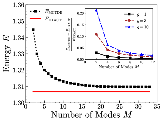
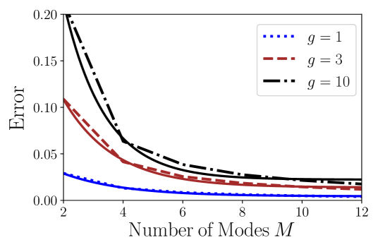
Figure 1: Top: Convergence of the ground state energy, calculated via MCTDH-X with increasing number of orbitals (black squares), $M=2,\dots,33$ towards the exact value from Eq. (4) (red solid); the coupling $g=1$. Inset: The relative error for the ground state energy for $g=1$ (black solid), $g=3$ (brown dashed) and $g=10$ (blue dash-dotted). Exact ground energies for different values of $g$ are $E_{g=1}=1.30675,E_{g=3}=1.59991,E_{g=10}=1.85069$. Bottom: Exponential fit for the relative error for the ground state (inset of the top figure).

4 Convergence of MCTDH to exact ground state energy

In order to verify convergence of the ground state energy to the exact result, we performed extensive MCTDH calculations for a wide range of the number of orbitals, $M=2,\dots,33$. In Fig. 1, we present the comparison between the exact and numerical values of the ground state energy for the interaction coupling $g=1$. We conclude that the numerical value converges rapidly for a large number of orbitals. The relative error between the exact and converged numerical values becomes less than $3$ ‰ when $M>15$. We however also notice that upon further increase of $M$, the error does not decrease significantly further. Specifically, for $M=20$ the error is $2.48$ ‰, and for $M=33$ it is still $2.26$ ‰. From Fig. 1 we see that for large $M$ the energy converges exponentially with a small relative error, corresponding to results of similar calculations that employed interaction rescaling, for a smaller number of orbitals, see Ref. [45]. To illustrate the dependence of the convergence on $g$, the relative error for the energy, ${(E_{\rm MCTDH}-E_{\rm exact})}/{E_{\rm exact}}$, is shown in the inset of Fig. 1 for $M=2,\dots,12$ and $g=1,3,$ and $10$. The bottom panel in Fig 1 shows the exponential fit of the relative error as a function of number of modes $M$ for intermediate ($g=1,3$) and strong ($g=10$) interaction strength, demonstrating that a similar behavior of the convergence is obtained for various $g$. The MCTDH calculations still converge reasonably well for sufficiently large $M$ to the exact energy. However, the computational cost (the $M$ needed for convergence) is, as expected, seen to increase for larger values of $g$.

5 Density matrix

Generally, correlation functions are more sensitive to the accuracy of MCTDH predictions than the ground state energy is, cf. [13, 14, 46]. Therefore, we now concentrate on a comparison of the analytics to numerics in the form of the first-order correlations, as encapsulated by the SPDM. We compare the results of our MCTDH calculations, in addition, with the Monte Carlo calculations performed by Minguzzi et al. in Ref. [34] for the SPDM of a pair of hard-core bosons in a 1D harmonic trap.The emphasis for this part of the paper is to assess the accuracy of MCTDH when $g$ in the Hamiltonian Eq. (1) is varied from weak over intermediate to strong coupling, so that we here fix $M=10$.

5.1 Real space

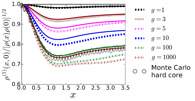
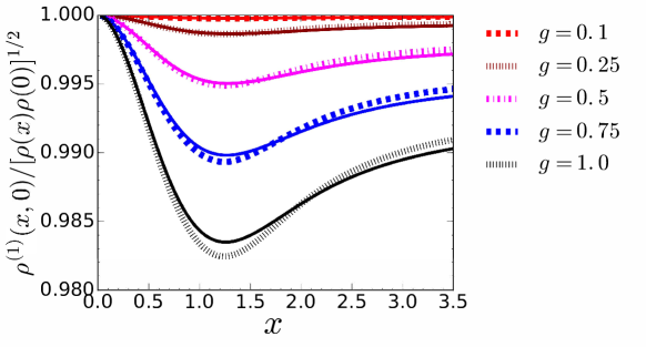
Figure 2: Top: SPDM $\rho^{(1)}(x,x^{\prime})/\sqrt{\rho(x)\rho(x^{\prime})}$ as a function of $x$ and $x^{\prime}=0$ for $N=2$ interacting bosons in a harmonic trap, in the strong coupling regime. The gray circles are the Monte Carlo results of Minguzzi et al. [34] for hard-core bosons ($g\rightarrow\infty$), with the size of the circles representing the error bars in the Monte Carlo data. The lines are MCTDH results for various $g$ and $M=10$. The solid lines show the analytical result. Bottom: Comparison of MCDTH results ($M=10$) with the 1D analytical solution in the range of intermediate interaction couplings.

In Fig. 2, we plot the normalized SPDM $\rho^{(1)}(x,x^{\prime})/\sqrt{\rho(x)\rho(x^{\prime})}$ as function of $x$, and at fixed $x^{\prime}=0$, for relatively large values of $g$. The gray circles in the top panel are taken from the Monte Carlo data of Ref. [34], while the solid lines show the comparison of MCTDH results with the 1D variant of the 3D analytical solution for $N=2$ bosons in a harmonic trap [32, 33]. We observe that the qualitative behavior of the MCTDH results is in accord with the analytical result as well as with the hard-core Monte Carlo calculations – the dip in the first-order correlations located at approximately $x=l$ is consistently visible. Note that this dip in the correlation function $\rho^{(1)}(x,x^{\prime})$ corresponds to a peak in phase fluctuations, defined according to [47] $\langle\hat{\psi^{\dagger}}(x)\hat{\psi}(x^{\prime})\rangle=\sqrt{\rho(x)\rho(x^{\prime})}\exp[-\frac{1}{2}\langle\hat{\delta\phi}_{xx^{\prime}}^{2}\rangle],$where $\hat{\delta\phi}_{xx^{\prime}}=\hat{\phi}(x)-\hat{\phi}(x^{\prime})$ is the phase difference operator and $\rho(x)=\langle\hat{\psi^{\dagger}}(x)\hat{\psi}(x)\rangle$ is the mean local density. For a more detailed discussion of phase fluctuations and their relation to the first-order correlations, we refer the reader to Ref. [47].

The correlation dip is due to the presence and geometry of the trap and, consequently, related to the shape of the occupied orbitals and exists even for relatively small interaction couplings. The built-in self-consistency of the MCTDH method is crucial in order to correctly describe the correlation phenomena in trapped quantum many-body systems, because the depth and location of the correlation dip sensitively depends on the self-consistently determined orbital shape.

We note in the top panel of Fig. 2 a sizable quantitative difference to the analytical solutions already for interaction strengths that are far below the hard-core limit of $g\rightarrow\infty$. However, for couplings commonly realized in experiments with magnetic traps (see for concrete estimates below), the agreement between the analytical results and MCTDH is very satisfactory, see the lower panel of Fig. 2, even for the relatively modest number of orbitals $M=10$ used in these calculations. The characteristic dip in the correlation function appears for any interaction strength and is correctly reproduced by the MCTDH method to good accuracy in its location, while the depth of the dip is somewhat exaggerated by MCTDH in particular for larger than intermediate couplings, $g\gg 1$.

5.2 Fourier space

An experimentally accessible quantity is the Fourier transform of the first-order correlation function [48]. In Fig. 3, we show the single-particle momentum density distribution, which is defined as a Fourier transform of the first-order correlation function in position space according to

$$\tilde{\rho}^{(1)}(k,k^{\prime})=\int dx\int dx^{\prime}\rho^{(1)}(x,x^{\prime})\exp[i(kx-k^{\prime}x^{\prime})]\\$$ (8)

for both the MCTDH result as well as the exact solution. The momentum density $\tilde{\rho}(k)$ is a Fourier transform of the spatial density $\rho(x)$ serves to normalize $\tilde{\rho}^{(1)}(k,k^{\prime})$. We see that, similarly to the real space SPDM, MCTDH and exact result agree quite well with each other, even for the very large values up to $g=1000$ we have addressed in our calculations.

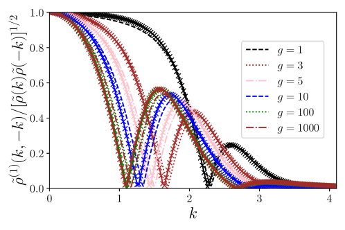
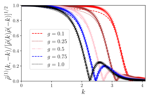
Figure 3: Normalized single-particle momentum density distribution, for various $g$ as indicated in the insets. The crosses are MCTDH results for various $g$ and $M=10$. The lines show the analytical result.

6 Fragmentation measure

6.1 Definition

Using the SPDM, one may formally define an important figure of merit, the fragmentation. By diagonalizing the SPDM, one obtains its eigenfunctions, $\phi_{i}$, and eigenvalues, $N_{i}$, which are in the many-body context referred to as natural orbitals and occupation numbers, respectively,

$$\rho^{(1)}(x,x^{\prime})=\sum_{i=0}^{M-1}N_{i}\phi^{\ast}_{i}(x^{\prime})\phi_{i}(x).$$ (9)

Here, the sum for MCTDH runs over the finite set $i=\{0,\ldots,M-1\}$ and for the exact solution over an infinite set $i=\{0,\ldots,\infty\}$.

The conventional definition of fragmentation [49] states that if a subset of the eigenvalues $N_{i}$ are “macroscopic,” i.e. some of the $n_{i}=N_{i}/N$ remain finite in the large $N$ limit, then the many-body state of the Bose gas is a simple or fragmented BEC when the cardinality of this subset is one or larger than one, respectively [50, 51]. This formal definition of fragmentation obviously cannot be applied in our case. We therefore define instead as the “degree of fragmentation’ the quantity

$$\mbox{Fragmentation}\qquad f\coloneqq\frac{N-N_{0}}{N},$$ (10)

that is, the relative occupation number of all orbitals excluding the most populated one (which has $i\coloneqq 0$), sorting occupation numbers $N_{i}$ from largest to smallest. The fragmentation thus defined represents a shorthand for the relative number of particles residing in all orbitals outside the most occupied one (the “condensate”). We note that in this definition we also take automatically into account the fact that the field operator truncation always has a finite number of modes $M$).

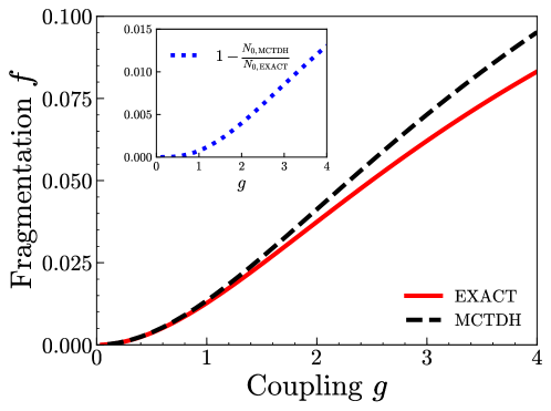
Figure 4: Fragmentation $f$ as defined in Eq. (10), obtained from the diagonalization of the analytical SPDM (red solid) and from MCTDH (black dashed) with $M=10$ orbitals, for the range $g=0.1,\dots,4$. The inset shows the relative numerical error in the occupation number of the energetically lowest orbital.

In Fig. 4, we display the exact fragmentation $f$ calculated using the exact density matrix in Eq. (6). We obtain the exact occupation numbers by first expressing $\rho^{(1)}(x,x^{\prime})$ in a harmonic oscillator eigenfunctions basis of dimension $M_{\rm ho}=50$ (which proved sufficiently large) and by then diagonalizing it, evaluating the integrals via the Gauss-Hermite approximation. The sizable difference when $g\gg 1$, is further illustrated in the inset, which shows the error in the occupation of the lowest orbital, $1-N_{0,{\rm MCTDH}}/N_{0,{\rm exact}}$. Note that the fragmentation $f$ obtained via MCTDH is always larger than the exact value, which is in agreement with the observation that the former approach overestimates the correlation dip in the first-order correlations (and hence also overestimates phase fluctuations), cf. Fig. 2.

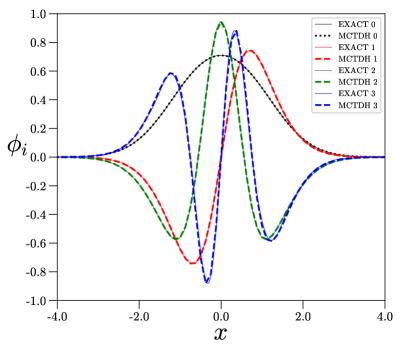
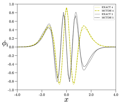
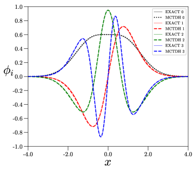
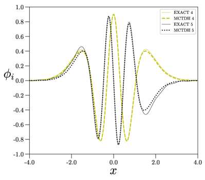
Figure 5: The first six natural orbitals $\phi_{i}(x)$, $i=0,\dots,5$, in Eq. (9), obtained via MCTDH (dashed, $M=10$) and the exact results (solid), from diagonalizing the SPDM in Eq. (6) (solid). Left: $i=0,\dots,3$, right: $i=4,5$. Top row: $g=1$, bottom row $g=10$.

6.2 Natural orbitals

In Fig. 5, we plot the first six natural orbitals contained in the diagonalized SPDM Eq. (9). We conclude that sizable deviations between exact and MCTDH natural orbitals start to occur for $i=4$ and above; within the resolution of the figure, we detected no discernible deviation in the first four, that is energetically lowest, natural orbitals, $i=0,\dots,3$, the exact and MCTDH curves lying precisely on top of each other in this range. We also note in this context that the occupation numbers $N_{i}$ for $i>2$ are very small. For example, $N_{3}$ is about an order of magnitude less than $N_{2}$, for both $g=1$ and $g=10$ and for both MCTDH and exact occupation numbers . Therefore, it is indeed the occupation number difference of the lower natural orbitals (rather than their precise shape) which explains the different fragmentation obtained by MCTDH and exact solution. As a corollary, going to much larger $M$ does not significantly decrease the degree of fragmentation $f$-difference further.

7 Conclusion

We now illustrate the above general considerations by inserting concrete numbers for an experimentally realizable parameter set. In a quasi-1D Bose gas, and far away from geometric resonances [53], we have $g=4a_{\rm sc}l/l_{\perp}^{2}$ where $l_{\perp}$ is the transverse trapping length. For ⁸⁷​Rb, this implies that the coupling $g=1.96\times a_{\rm sc}[a_{\rm Rb}]\nu_{\perp}[{\rm kHz}]/\sqrt{\nu[{\rm Hz}]}$, where the background scattering length $a_{\rm Rb}=5.29$ nm, $\omega_{\perp,\nu}=2\pi\nu_{\perp,\nu}$, and the frequencies are scaled with typical experimental values see, e.g., [54, 55]. With the background scattering length of ⁸⁷​Rb, and $g\sim{\cal O}(1)$, the MCTDH results are in satisfactory accord with the analytical result for quasi-1D setups accessible by magnetic trapping.

Limits of the MCTDH approach can be explored, e.g., in optical lattices when one increases $g$ towards the Tonks-Girardeau regime [36, 37]. While only at a filling of two per one-dimensional tube our results can strictly be applied, we anticipate that also for larger $N$ qualitatively similar features as those in Fig. 2, and in particular the trap-induced correlation dip, should persist and be observable for example with (a combination of) Feshbach resonances [41] and higher aspect ratios. Variation of $g$ and $N$ and measurement of, e.g., the first-order correlations which have been investigated here paves the way for a quantitative experimental assessment of the accuracy and convergence of MCTDH. The detailed analysis of higher-order correlations [56] will then reveal further precise information on the applicability of the MCTDH method to strongly correlated systems and probe its range of applicability.

References

- Meyer et al. [1990] H.-D. Meyer, U. Manthe, and L. S. Cederbaum, “The multi-configurational time-dependent Hartree approach,” Chemical Physics Letters 165, 73–78 (1990).
- Meyer et al. [2009] H.-D. Meyer, F. Gatti, and G. A. Worth, eds., Multidimensional Quantum Dynamics: MCTDH Theory and Applications (John Wiley & Sons, 2009).
- Alon et al. [2008] Ofir E. Alon, Alexej I. Streltsov, and Lorenz S. Cederbaum, “Multi-configurational time-dependent Hartree method for bosons: Many-body dynamics of bosonic systems,” Phys. Rev. A 77, 033613 (2008).
- [4] A. U. J. ”Lode, M. Tsatsos, E. Fasshauer, Papariello L. Lin, R., P. Molignini, Lévêque. C., and Weiner S. E.”, “MCTDH-X: The time-dependent multiconfigurational Hartree for indistinguishable particles software,” http://ultracold.org.
- Lin et al. [2020] Rui Lin, Paolo Molignini, Luca Papariello, Marios C. Tsatsos, Camille Lévêque, Storm E. Weiner, Elke Fasshauer, R. Chitra, and Axel U.J. Lode, “MCTDH-X: The multiconfigurational time-dependent Hartree method for indistinguishable particles software,” Quantum Science and Technology, 5, 024004 (2020).
- Beck et al. [2000] M. H. Beck, A. Jäckle, G. A. Worth, and H.-D. Meyer, “The multiconfiguration time-dependent Hartree (MCTDH) method: a highly efficient algorithm for propagating wavepackets,” Physics Reports 324, 1–105 (2000).
- Lode et al. [2012] Axel U. J. Lode, Kaspar Sakmann, Ofir E. Alon, Lorenz S. Cederbaum, and Alexej I. Streltsov, “Numerically exact quantum dynamics of bosons with time-dependent interactions of harmonic type,” Phys. Rev. A 86, 063606 (2012).
- Grond et al. [2013] Julian Grond, Alexej I. Streltsov, Axel U. J. Lode, Kaspar Sakmann, Lorenz S. Cederbaum, and Ofir E. Alon, “Excitation spectra of many-body systems by linear response: General theory and applications to trapped condensates,” Phys. Rev. A 88, 023606 (2013).
- Streltsov [2013] Alexej I. Streltsov, “Quantum systems of ultracold bosons with customized interparticle interactions,” Phys. Rev. A 88, 041602 (2013).
- Fischer et al. [2015] Uwe R. Fischer, Axel U. J. Lode, and Budhaditya Chatterjee, “Condensate fragmentation as a sensitive measure of the quantum many-body behavior of bosons with long-range interactions,” Phys. Rev. A 91, 063621 (2015).
- Krönke and Schmelcher [2015] Sven Krönke and Peter Schmelcher, “Two-body correlations and natural-orbital tomography in ultracold bosonic systems of definite parity,” Phys. Rev. A 92, 023631 (2015).
- Krönke and Schmelcher [2018] Sven Krönke and Peter Schmelcher, “Born-Bogoliubov-Green-Kirkwood-Yvon hierarchy for ultracold bosonic systems,” Phys. Rev. A 98, 013629 (2018).
- Klaiman and Alon [2015] Shachar Klaiman and Ofir E. Alon, “Variance as a sensitive probe of correlations,” Phys. Rev. A 91, 063613 (2015).
- Klaiman and Cederbaum [2016] Shachar Klaiman and Lorenz S. Cederbaum, “Overlap of exact and Gross-Pitaevskii wave functions in Bose-Einstein condensates of dilute gases,” Phys. Rev. A 94, 063648 (2016).
- Sakmann and Kasevich [2016] Kaspar Sakmann and Mark Kasevich, “Single-shot simulations of dynamic quantum many-body systems,” Nature Physics 12, 451–454 (2016).
- Lode and Bruder [2017] Axel U. J. Lode and Christoph Bruder, “Fragmented Superradiance of a Bose-Einstein Condensate in an Optical Cavity,” Phys. Rev. Lett. 118, 013603 (2017).
- Nguyen et al. [2019] J. H. V. Nguyen, M. C. Tsatsos, D. Luo, A. U. J. Lode, G. D. Telles, V. S. Bagnato, and R. G. Hulet, “Parametric Excitation of a Bose-Einstein Condensate: From Faraday Waves to Granulation,” Phys. Rev. X 9, 011052 (2019).
- Lode et al. [2020] Axel U. J. Lode, Camille Lévêque, Lars Bojer Madsen, Alexej I. Streltsov, and Ofir E. Alon, “Colloquium: Multiconfigurational time-dependent Hartree approaches for indistinguishable particles,” Rev. Mod. Phys. 92, 011001 (2020).
- [19] P. D. Drummond and J. Brand, “Comment on: ‘Single-shot simulations of dynamic quantum many-body systems’,” arXiv:1610.07633 [cond-mat.quant-gas] .
- [20] K. Sakmann and M. Kasevich, “Reply to the correspondence of Drummond and Brand [arXiv:1610.07633],” arXiv:1702.01211 [cond-mat.quant-gas] .
- [21] M. K. Olsen, J. F. Corney, R. J. Lewis-Swan, and A. S. Bradley, “Correspondence on “Single-shot simulations of dynamic quantum many-body systems”,” arXiv:1702.00282 [quant-ph] .
- Cosme et al. [2016] Jayson G. Cosme, Christoph Weiss, and Joachim Brand, “Center-of-mass motion as a sensitive convergence test for variational multimode quantum dynamics,” Phys. Rev. A 94, 043603 (2016).
- Manthe [2015] Uwe Manthe, “The multi-configurational time-dependent Hartree approach revisited,” The Journal of Chemical Physics 142, 244109 (2015).
- Kloss et al. [2017] Benedikt Kloss, Irene Burghardt, and Christian Lubich, “Implementation of a novel projector-splitting integrator for the multi-configurational time-dependent Hartree approach,” The Journal of Chemical Physics 146, 174107 (2017).
- Meyer and Wang [2018] Hans-Dieter Meyer and Haobin Wang, “On regularizing the MCTDH equations of motion,” The Journal of Chemical Physics 148, 124105 (2018).
- Lee and Fischer [2014] Kang-Soo Lee and Uwe R. Fischer, “Truncated many-body dynamics of interacting bosons: A variational principle with error monitoring,” International Journal of Modern Physics B 28, 1550021 (2014).
- Drummond and Opanchuk [2017] Peter D. Drummond and Bogdan Opanchuk, “Truncated Wigner dynamics and conservation laws,” Phys. Rev. A 96, 043616 (2017).
- Castin and Dum [1998] Y. Castin and R. Dum, “Low-temperature Bose-Einstein condensates in time-dependent traps: Beyond the symmetry-breaking approach,” Phys. Rev. A 57, 3008–3021 (1998).
- Cederbaum [2017] Lorenz S. Cederbaum, “Exact many-body wave function and properties of trapped bosons in the infinite-particle limit,” Phys. Rev. A 96, 013615 (2017).
- Lieb and Seiringer [2002] Elliott H. Lieb and Robert Seiringer, “Proof of Bose-Einstein Condensation for Dilute Trapped Gases,” Phys. Rev. Lett. 88, 170409 (2002).
- Lieb et al. [2003] Elliott H. Lieb, Robert Seiringer, and Jakob Yngvason, “One-Dimensional Bosons in Three-Dimensional Traps,” Phys. Rev. Lett. 91, 150401 (2003).
- Busch et al. [1998] Thomas Busch, Berthold-Georg Englert, Kazimierz Rza̧żewski, and Martin Wilkens, “Two Cold Atoms in a Harmonic Trap,” Foundations of Physics 28, 549–559 (1998).
- Idziaszek and Calarco [2006] Zbigniew Idziaszek and Tommaso Calarco, “Analytical solutions for the dynamics of two trapped interacting ultracold atoms,” Phys. Rev. A 74, 022712 (2006).
- Minguzzi et al. [2002] A. Minguzzi, P. Vignolo, and M. P. Tosi, “High-momentum tail in the Tonks gas under harmonic confinement,” Physics Letters A 294, 222–226 (2002).
- Cazalilla et al. [2011] M. A. Cazalilla, R. Citro, T. Giamarchi, E. Orignac, and M. Rigol, “One dimensional Bosons: From Condensed Matter Systems to Ultracold Gases,” Rev. Mod. Phys. 83, 1405–1466 (2011).
- Paredes et al. [2004] Belén Paredes, Artur Widera, Valentin Murg, Olaf Mandel, Simon Fölling, Ignacio Cirac, Gora V Shlyapnikov, Theodor W Hänsch, and Immanuel Bloch, “Tonks-Girardeau gas of ultracold atoms in an optical lattice.” Nature 429, 277 (2004).
- Kinoshita et al. [2004] Toshiya Kinoshita, Trevor Wenger, and David S Weiss, “Observation of a one-dimensional Tonks-Girardeau gas,” Science 305, 1125 (2004).
- Lieb and Liniger [1963] Elliott H. Lieb and Werner Liniger, “Exact Analysis of an Interacting Bose Gas. I. The General Solution and the Ground State,” Phys. Rev. 130, 1605–1616 (1963).
- Sakmann et al. [2009] Kaspar Sakmann, Alexej I. Streltsov, Ofir E. Alon, and Lorenz S. Cederbaum, “Exact Quantum Dynamics of a Bosonic Josephson Junction,” Phys. Rev. Lett. 103, 220601 (2009).
- [40] An exactly solvable model (which is readily integrable for any ) and the convergence of MCTDH towards its solutions was studied with a harmonic interaction potential in Ref. [7], with the obvious limitation that this interaction is not realized in ultracold atomic gases.
- Chin et al. [2010] Cheng Chin, Rudolf Grimm, Paul Julienne, and Eite Tiesinga, “Feshbach resonances in ultracold gases,” Reviews of Modern Physics 82, 1225–1286 (2010).
- Abramowitz and Stegun [1970] M. Abramowitz and I. A. Stegun, Handbook of mathematical functions (Dover Publications, New York, 1970).
- Lode [2016] Axel U. J. Lode, “Multiconfigurational time-dependent Hartree method for bosons with internal degrees of freedom: Theory and composite fragmentation of multicomponent Bose-Einstein condensates,” Phys. Rev. A 93, 063601 (2016).
- Fasshauer and Lode [2016] Elke Fasshauer and Axel U. J. Lode, “Multiconfigurational time-dependent Hartree method for fermions: Implementation, exactness, and few-fermion tunneling to open space,” Phys. Rev. A 93, 033635 (2016).
- Ernst et al. [2011] Thomas Ernst, David W. Hallwood, Jake Gulliksen, Hans-Dieter Meyer, and Joachim Brand, “Simulating strongly correlated multiparticle systems in a truncated Hilbert space,” Phys. Rev. A 84, 023623 (2011).
- Klaiman et al. [2018] Shachar Klaiman, Raphael Beinke, Lorenz S. Cederbaum, Alexej I. Streltsov, and Ofir E. Alon, “Variance of an anisotropic Bose-Einstein condensate,” Chemical Physics 509, 45–54 (2018).
- Marchukov and Fischer [2019] Oleksandr V. Marchukov and Uwe R. Fischer, “Self-consistent determination of the many-body state of ultracold bosonic atoms in a one-dimensional harmonic trap,” Annals of Physics 405, 274–288 (2019).
- Cohen-Tannoudji [2011] C. Cohen-Tannoudji, “Coherence properties of Bose-Einstein condensates,” in Advances in Atomic Physics (World Scientific, 2011) pp. 577–602.
- Penrose and Onsager [1956] Oliver Penrose and Lars Onsager, “Bose-Einstein Condensation and Liquid Helium,” Phys. Rev. 104, 576–584 (1956).
- Leggett [2001] Anthony J. Leggett, “Bose-Einstein condensation in the alkali gases: Some fundamental concepts,” Rev. Mod. Phys. 73, 307–356 (2001).
- Mueller et al. [2006] Erich J. Mueller, Tin-Lun Ho, Masahito Ueda, and Gordon Baym, “Fragmentation of Bose-Einstein condensates,” Phys. Rev. A 74, 033612 (2006).
- Note [1] Specifically, for , (exact), (MCTDH, ), (MCTDH, ), while (exact), (MCTDH, ), (MCTDH, ).
- Olshanii [1998] Maxim Olshanii, “Atomic Scattering in the Presence of an External Confinement and a Gas of Impenetrable Bosons,” Phys. Rev. Lett. 81, 938 (1998).
- Betz et al. [2011] T. Betz, S. Manz, R. Bücker, T. Berrada, Ch. Koller, G. Kazakov, I. E. Mazets, H.-P. Stimming, A. Perrin, T. Schumm, and J. Schmiedmayer, “Two-Point Phase Correlations of a One-Dimensional Bosonic Josephson Junction,” Phys. Rev. Lett. 106, 020407 (2011).
- Fang et al. [2016] Bess Fang, Aisling Johnson, Tommaso Roscilde, and Isabelle Bouchoule, “Momentum-Space Correlations of a One-Dimensional Bose Gas,” Phys. Rev. Lett. 116, 050402 (2016).
- Schweigler et al. [2017] Thomas Schweigler, Valentin Kasper, Sebastian Erne, Igor Mazets, Bernhard Rauer, Federica Cataldini, Tim Langen, Thomas Gasenzer, Jürgen Berges, and Jörg Schmiedmayer, “Experimental characterization of a quantum many-body system via higher-order correlations,” Nature 545, 323–326 (2017).