On the Performance and Convergence of Distributed Stream Processing via Approximate Fault Tolerance ††thanks: An earlier version of the paper appeared in [39]. In this extended version, we formally prove that AF-Stream preserves the convergence guarantees of online learning in distributed stream processing, and also validate our convergence analysis through prototype experiments for different datasets, parameters, and consistency models.
Abstract
Fault tolerance is critical for distributed stream processing systems, yet achieving error-free fault tolerance often incurs substantial performance overhead. We present AF-Stream, a distributed stream processing system that addresses the trade-off between performance and accuracy in fault tolerance. AF-Stream builds on a notion called approximate fault tolerance, whose idea is to mitigate backup overhead by adaptively issuing backups, while ensuring that the errors upon failures are bounded with theoretical guarantees. Specifically, AF-Stream allows users to specify bounds on both the state divergence and the loss of non-backup streaming items. It issues state and item backups only when the bounds are reached. Our AF-Stream design provides an extensible programming model for incorporating general streaming algorithms as well as exports only few threshold parameters for configuring approximation fault tolerance. Furthermore, we formally prove that AF-Stream preserves high algorithm-specific accuracy of streaming algorithms, and in particular the convergence guarantees of online learning. Experiments show that AF-Stream maintains high performance (compared to no fault tolerance) and high accuracy after multiple failures (compared to no failures) under various streaming algorithms.
1 Introduction
Stream processing becomes an important paradigm for processing data at high speed and large scale. As opposed to traditional batch processing that is designed for static data, stream processing treats data as a continuous stream, and processes every item in the stream in real-time. For scalability, we can make stream processing distributed, by processing streaming items in parallel through multiple processes (or workers) or threads.
Given that failures can happen at any time and at any worker in a distributed environment, fault tolerance is a critical requirement in distributed stream processing. In particular, streaming algorithms often keep internal states in main memory, which is fast but unreliable. Also, streaming items are generated continuously in real-time, and will become unavailable after being processed. Thus, we need to provide fault tolerance guarantees for both internal states and streaming items. Most existing stream processing systems (e.g., Spark Streaming [80] and Apache Flink [19]) support error-free fault tolerance and exactly-once message delivery semantics. They issue regular backups for both internal states and streaming items, so that when failures happen, they can recover from the most recent backup and resume processing as normal. However, frequent backups incur significant network and disk I/Os, thereby degrading stream processing performance. Some stream processing systems (e.g., Storm [73] and Heron [45]) support best-effort fault tolerance and at-most-once message delivery semantics to trade recovery accuracy for performance, but the drawback is that they can incur unbounded errors that compromise the correctness of outputs when recovering from failures.
We propose AF-Stream, a distributed stream processing system that addresses the trade-off between performance and accuracy in fault tolerance. AF-Stream builds on a notion called approximate fault tolerance, whose idea is to adaptively issue backup operations for both internal states and unprocessed items, while incurring only bounded errors after failures are recovered. Specifically, AF-Stream estimates the errors upon failures with the aid of extensible programming interfaces, and issues a backup operation only when the errors go beyond the user-specified acceptable level.
We justify the trade-off with two observations. First, to mitigate computational complexities, streaming algorithms tend to produce “quick-and-dirty” results rather than exact ones (e.g., data synopsis) (§2.2). It is thus feasible to incur small additional errors due to approximate fault tolerance, provided that the errors are bounded. Such errors can often be amortized after the processing of large-volume and high-speed data streams. Second, although failures are prevalent in distributed systems, their occurrences remain relatively infrequent over the lifetime of stream processing. Thus, incurring errors upon failures should bring limited disturbance. We point out that the power of approximation has been extensively addressed in distributed computing (e.g., [2, 47, 63, 3, 60, 76, 77]). To our knowledge, AF-Stream is the first work that leverages approximation to achieve fault tolerance in distributed stream processing with bounded error guarantees. Our contributions are summarized as follows.
First, AF-Stream provides an extensible programming model for general streaming algorithms. In particular, it exports built-in interfaces and primitives that make fault tolerance intrinsically supported and transparent to programmers.
Second, AF-Stream realizes approximate fault tolerance, which bounds errors upon failures in two aspects: state divergence and number of lost items. We prove that the errors are bounded independent of the number of failures and the number of workers in a distributed environment. Also, the error bounds are tunable with only three user-configurable threshold parameters to trade between performance and accuracy. We give examples on how such parameters correspond to the error bounds of streaming algorithms. Note that AF-Stream adds no error to the common case when no failure happens.
Third, we analyze how AF-Stream affects the model convergence of online learning under approximate fault tolerance. We formally prove that AF-Stream preserves the iterative-convergent and error-tolerant nature of online learning [14, 25] after recovering from multiple failures. Our analysis focuses on stochastic gradient descent [12], a core primitive for many popular online learning algorithms [13].
Fourth, we implement an AF-Stream prototype, with emphasis on optimizing its inter-thread and inter-worker communications. Our AF-Stream prototype also supports different consistency models.
Finally, we evaluate the performance and accuracy of our AF-Stream prototype on Amazon EC2 and a local cluster for various streaming algorithms. AF-stream only degrades the throughput by up to 4.7%, 5.2%, and 0.3% in heavy hitter detection, online join, and online logistic regression, respectively, when compared to disabling backups; meanwhile, its accuracy after 10 failures only drops by a small percentage (based on algorithm-specific metrics) when compared to without failures. Also, for online logistic regression, AF-Stream only slightly delays model convergence (e.g., by 13.3% and 20% for two real-world traces under eight failures).
The source code of our AF-Stream prototype is available at: http://adslab.cse.cuhk.edu.hk/software/afstream.
2 Streaming Algorithms
We first provide an overview of general streaming algorithms. We then focus on three classes of streaming algorithms, and identify their commonalities to guide our system design.
2.1 Overview and Motivation
A streaming algorithm comprises a set of operators for processing a data stream of items. Each operator continuously receives an input item, processes the item, and produces one or multiple output items. It also keeps an in-memory state, which holds a collection of values corresponding to the processing of all received input items. The state is updated after each input item is processed. Also, an operator produces new items with respect to the updated state.
If failures never happen, we refer to the produced state and output as the ideal state and ideal output, respectively. However, the actual deployment environment is failure-prone. In this case, an operator needs to generate its actual state and actual output in a fault-tolerant manner. Specifically, an operator needs to handle: (i) the missing in-memory state and (ii) missing unprocessed items.
Suppose that we want to achieve error-free fault tolerance for an operator. That is, we ensure that the actual state and output are identical to the ideal state and output, respectively, after the recovery of a failure. This necessitates the availability of a prior state and any following items, so that when a failure happens, we can retrieve the prior state and resume the processing of the following items. In particular, in stream processing, the items to be processed are generated continuously, so we need to issue periodic state backups and a backup for every item in order to achieve error-free fault tolerance. For example, Spark Streaming saves each state as a Resilient Distributed Dataset (RDD) [80] in a mini-batch fashion and saves each item via write-ahead logging [81].
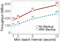
However, making regular backups for both the state and each item incurs excessive I/O overhead to normal processing. We motivate this claim by evaluating the backup overhead of Spark Streaming (v1.4.1) versus the mini-batch interval (i.e., the duration within which items are batched). Note that the performance of Spark Streaming is sensitive to the number of items in a mini-batch: having small mini-batches aggravates backup overhead, while having very large mini-batches increases the processing time to even exceed the mini-batch interval and makes the system unstable (i.e., the system throughput varies significantly) [26]. Thus, for each given mini-batch interval, we tune the stream input rate that gives the maximum stable throughput. Figure 1 shows the throughput of Spark Streaming for Grep and WordCount, measured on Amazon EC2 (see §6 for the details on the datasets and experimental setup). We see that the throughput drops significantly due to backups, for example, by nearly 50% for WordCount when the mini-batch interval is 1s.

|
 |
| (a) Grep | (b) WordCount |
| Grep | WordCount | |
| No fault tolerance | 275.83 MB/s | 149.24 MB/s |
| With state backup only | 263.78 MB/s | 118.41 MB/s |
| With item backup only | 136.81 MB/s | 82.18 MB/s |
| With both state and item backups | 98.75 MB/s | 76.76 MB/s |
We also study the fault tolerance overhead in Apache Flink (v1.7.2) [19] on a local cluster (see §6 for the cluster setup). Flink issues state backups as checkpoints. For item backups, we persist items in Kafka [7], which we configure as a reliable data source for Flink; if item backups are disabled, we load the whole dataset into RAM to mitigate the I/O overhead (see Section 6.1.1 for more evaluation on the use of Kafka). Table 1 shows the throughput of Grep and WordCount with different fault tolerance approaches. Enabling both state and item backups can drop the throughput by 64% and 49% in Grep and WordCount, respectively, compared to without fault tolerance.
2.2 Classes of Streaming Algorithms
This paper focuses on three classes of streaming algorithms that have been well studied and widely deployed.
Data synopsis.
Data synopsis algorithms summarize vital information of large-volume data streams into compact in-memory data structures with low time and space complexities. Examples include sampling, histograms, wavelets, and sketches [22], and have been used in areas such as anomaly detection in network traffic [28, 23] and social network analysis [67]. To bound the memory usage of data structures, data synopsis algorithms are often designed to return estimates with bounded errors. For example, sampling algorithms (e.g., [28]) perform computations on a subset of items; sketch-based algorithms (e.g., [28, 23]) map a large key space into a fixed-size two-dimensional array of counters.
Stream database queries.
Stream databases manage data streams with SQL-like operators as in traditional relational databases, and allow queries to be continuously executed over continuous streams. Since some SQL operators (e.g., join, sorting, etc.) require multiple iterations to process items, stream database queries need to adapt the semantics of SQL operators for stream processing. For example, they restrict the processing of items over a time window, or return approximate query results using data synopsis techniques (e.g., sampling in online join queries [32, 52]).
Online learning.
Machine learning aims to model the properties of data by processing the data (possibly over iterations) and identifying the optimal parameters toward some objective function. It has been widely used in web search, advertising, and analytics.
Traditional machine learning algorithms assume that the whole dataset is available in advance and iteratively refine parameters towards a global optimization objective on the whole dataset. To support stream processing, online learning algorithms define a local objective function with respect to the current model parameter values, and search for the model parameter values that optimize the local objective function. After a large number of items are processed, it has been shown that the local approach can converge to a global optimal point, subject to certain conditions [83, 36, 37].
| Common features | Corresponding design choices |
| Common primitive operators | AF-Stream abstracts a streaming algorithm into a set of operators and maintains fault tolerance for each operator (§3.2). It also realizes a rich set of built-in primitive operators (§5). |
| Intensive and skewed state updates | AF-Stream supports partial state backup to reduce the backup size (§3.4.1). It also exposes interfaces to let users specify which parts of a state are actually included in a backup (§3.3). |
| Bounding by windows | AF-Stream resets thresholds based on windows (§3.5.2). It also exposes interfaces to let users specify window types and lengths (§3.3). |
2.3 Common Features
We identify the common features of existing streaming algorithms to be addressed in our system design. Table 2 shows how our design choices are related to the common features.
Common primitive operators.
We can often decompose an operator of a streaming algorithm into a number of primitive operators, which form the building blocks of the same class of streaming algorithms. For example, stream database queries are formed by few operators such as map, union, and join [1, 31, 61]; sketch-based algorithms are formed by hash functions, matching, and numeric arrays [79].
Intensive and skewed updates.
The state of an operator often holds update-intensive values, such as sketch counters [79] and model parameters in online learning [47]. Also, state values are updated at different frequencies. For example, the counters corresponding to frequent items are updated at higher rates; in online learning, only few model parameters are frequently updated due to the sparsity nature of machine learning features [47].
Bounding by windows.
2.4 Distributed Implementation
We can parallelize a streaming algorithm via distributed implementation. We identify two common distributed approaches, which can be used individually or in combination.
Pipelining.
It divides an operator into multiple stages, each of which corresponds to an operator or a primitive operator (§2.3). The output items of one stage can serve as input items to the next stage, while different stages can process different items in parallel.
Operator duplication.
It parallelizes stream processing via multiple copies of the same operator. There are two ways to distribute loads across operator copies: data partitioning, in which each operator copy processes a subset of items of a stream, and state partitioning, in which each operator copy manages a subset of values of a state. Both approaches can be used simultaneously in a streaming algorithm.
3 AF-Stream Design
AF-Stream abstracts a streaming algorithm as a set of operators. It maintains fault tolerance for each operator by making backups for its state and unprocessed items. To realize approximate fault tolerance, AF-Stream issues a backup operation only when the actual state and output deviate much from the ideal state and output, respectively. This mitigates backup overhead, while incurring bounded errors after failures are recovered.
AF-Stream’s approximate fault tolerance inherently differs from existing backup-based approaches for distributed stream processing. Unlike the approaches that achieve error-free fault tolerance (e.g., [42, 5, 61]), AF-Stream issues fewer backups, thereby improving stream processing performance. In addition, unlike the approaches that achieve best-effort fault tolerance by also making fewer backups (e.g., [57, 69]), AF-Stream ensures that the errors are bounded with theoretical guarantees. AF-Stream also differs from existing approximate processing systems (§7) in that it only applies approximation in maintaining fault tolerance rather than in normal processing.
3.1 Design Assumptions
To bound the errors upon failures, AF-Stream makes the following assumptions on streaming algorithms.
AF-Stream assumes that a single lost item (without any backup) brings limited degradations to accuracy. Instead of focusing on identifying a specific item (e.g., finding an outlier item), AF-Stream is designed to analyze the aggregated behavior over a large-volume stream of items, so each item has limited impact on the overall analysis. For example, in network monitoring, we may want to identify the flows whose sums of packet sizes exceed a threshold. Each item corresponds to a packet, whose maximum size is typically limited by the network (e.g., 1,500 bytes). Note that this assumption is also made by existing stream processing systems that build on approximation techniques (§7).
Note that after we recover a failed operator, there may be errors when the restored operator resumes processing from an actual state instead of from the ideal state. Nevertheless, such errors can often be amortized or compensated after processing a sufficiently large number of items. For example, online learning algorithms can converge to the optimal solution even if they start from a non-ideal state [46, 66, 35]. Thus, this type of errors brings limited accuracy degradations, as also validated by our experiments (§6).
Finally, AF-Stream assumes that the errors across multiple duplicate operator copies can be aggregated. For example, machine learning algorithms maintain linearly additive states [47], thereby allowing the errors of multiple copies to be summable.
3.2 Architecture
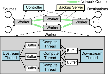
Figure 2 shows the architecture of AF-Stream. AF-Stream comprises multiple processes, including a single controller and multiple workers. Each worker manages a single operator of a streaming algorithm, while the controller coordinates the executions of all workers. AF-stream organizes workers as a graph, in which one or multiple sources originate data streams, and one or multiple destinations store the final results. For a pair of neighboring workers, say and , we call an upstream worker and a downstream worker if the stream processing directs from to . Specifically, a worker receives input items from either a source or an upstream worker, processes the items, and forwards output items to either a destination or a downstream worker.
AF-Stream also supports the feedback mechanism, which is essential for some streaming algorithms (e.g., model convergence in online learning [46]). It allows a downstream worker to optionally send feedback messages to an upstream worker. In other words, the communication between each pair of neighboring workers is bi-directional.
The controller manages the execution of each worker, which periodically sends heartbeats to the controller. If a worker fails, the controller recovers the failed state and data in a new worker. Also, each worker issues backups to a centralized backup server, which keeps backups in reliable storage. The backup server should be viewed as a logical entity that can be substituted with any external storage system (e.g., HDFS [65]). In this paper, we assume that the controller and the backup server are always available and have sufficient computational resources, yet we can deploy multiple controllers and backup servers for fault tolerance and scalability.
Each worker in AF-Stream comprises one upstream thread, one downstream thread, and multiple compute threads. The upstream thread forwards input items from either a source or an upstream worker to one of the compute threads, while the downstream thread forwards the output items from the compute threads to either a destination or a downstream worker. In particular, multiple compute threads can collaboratively process items, such that a compute thread can partially process an item and forward the intermediate results to another compute thread for further processing. Furthermore, the downstream thread can collect and forward any feedback message from a downstream worker to the compute threads for processing, and the upstream thread can forward any new feedback message from the compute threads to an upstream worker. Our implementation experience is that it suffices to have only one upstream thread and one downstream thread per worker to achieve the required processing performance. Thus, we can reserve the remaining CPU cores for compute threads to perform heavy-weight computations.
AF-Stream connects workers and threads as follows. For inter-worker communications, it connects each pair of upstream and downstream workers via a bi-directional network queue. For inter-thread communications, it shares data across threads via in-memory circular ring buffers. We carefully optimize both network queue and ring buffer implementations so as to mitigate the communication overhead (§5).
3.3 Programming Model
AF-Stream manages two types of objects: states and items (§2.1), whose formats are user-defined. Each operator is associated with a state111We also allow an operator to maintain an empty state (i.e., stateless)., and each state holds an array of binary values. Also, each operator supports three types of items: (i) data items, which collectively refer to the input and output items that traverse along workers from upstream to downstream in stream processing, (ii) feedback items, which traverse along workers from downstream to upstream, and (iii) punctuation items, which specify the end of an entire stream or a sub-stream for windowing (§2.3).
AF-Stream has two sets of interfaces: composing interfaces and user-defined interfaces, as listed in Appendix C. The composing interfaces are used to define the AF-Stream architecture and the stream processing workflows. Their functionalities can be summarized as follows: (i) connecting workers (in server hostnames) and the source/destination (in file pathnames), (ii) adding threads to each worker, (iii) connecting threads within each worker, (iv) pinning a thread to a CPU core, and (v) specifying the windowing type (e.g., hopping window, sliding window, decaying window) and window length.
On the other hand, user-defined interfaces allow programmers to add specific implementation details. AF-Stream automatically calls the user-defined interfaces and processes items based on their implementations. Specifically, the upstream thread can be customized to receive items, dispatch them to the compute threads, and optionally send feedback items to upstream workers. Similarly, the downstream thread can be customized to send output items and optionally receive feedback items from downstream workers. The compute thread can be customized to process data items, feedback items, and punctuation items.
AF-Stream provides three user-defined interfaces for building operators that realize approximate fault tolerance for state backup (§3.4.1): (i) StateDivergence, which quantifies the divergence between the current state and the most recent backup state, (ii) BackupState, by which operators provide the state to be saved in reliable storage via the backup server, and (iii) RecoverState, by which operators obtain the most recent backup state from the backup server. Such interfaces are included in a base class called FTOperator, which can be extended by specific fault-tolerant operators. By default, the three interfaces have empty implementations, meaning that state backup is disabled.
For example, Listing 1 shows the code snippet of a fault-tolerant hashmap FTHashMap, which extends the base class FTOperator. In the implementation, StateDivergence can specify the divergence of the hash map (e.g., in Listing 1, we use the Manhattan distance of counter values between the current and backup hash maps). BackupState can issue backups for the counter values in the hashmap, while RecoverState can restore the hashmap. Here, we assume that the backup hashmap is stored in a backup server. Note that BackupState and RecoverState also update the current backup hashmap in bkup_map for the computation of the state divergence in StateDivergence. We further elaborate how the functions are called in §3.4.1.
3.4 Approximate Fault Tolerance
AF-Stream maintains approximate fault tolerance for both the state and items of each operator. We introduce both state backup (§3.4.1) and item backup (§3.4.2) as individual backup mechanisms that are complementary to each other and are configured by different thresholds.
3.4.1 State Backup
Recall that AF-Stream calls BackupState to issue a backup operation for the state of an operator to the backup server. Instead of making frequent calls to BackupState, AF-Stream defers the call to BackupState until the current state deviates from the most recent backup state by some threshold (denoted by ). Specifically, AF-Stream caches a copy of the most recent backup state of the operator in local memory. Each time when an item updates the current state, AF-Stream calls StateDivergence to compute the divergence between the current state and the cached backup state. If the divergence exceeds , AF-Stream calls BackupState to issue a backup for the current state, and updates the cached copy accordingly.
Making the backup of an entire state may be expensive, especially if the state is large. To further mitigate backup overhead, AF-Stream supports the backup of a partial state, such that programmers can only specify the list of updated values (together with their indices) that make a state substantially deviate as the returned state of BackupState. Partial state backup is useful when only few values of a state are updated (§2.3).
Each state update triggers a call to StateDivergence. For most operators and divergence functions (e.g., difference of cardinalities, Manhattan distance, Euclidean distance, or maximum difference of values), StateDivergence only involves few arithmetic operations. For example, suppose that a divergence function returns the sum of differences (denoted by ) of all values between two states. If we update a value, then we can compute the new sum of differences (denoted by ) as , where is the change of the value. Thus, if the operator has only one compute thread, the compute thread itself can evaluate the divergence with limited overhead. On the other hand, if the operator has multiple compute threads to process a state simultaneously, say by operator duplication (§2.4), then summing the divergence of all compute threads can be expensive due to inter-thread communications. AF-Stream currently employs a smaller threshold in each compute thread, such that the sum of the thresholds does not exceed . For example, we can set the threshold as if there are compute threads.
3.4.2 Item Backup
AF-Stream makes item backups selective, such that a worker decides to make a backup for an item based on the item type and a pre-defined threshold. For a punctuation item, a worker always makes a backup for it to accurately identify the head and tail of a sequence to be processed; for a data item or a feedback item, the worker counts the number of pending items that have not yet been processed. If the number exceeds a threshold (denoted by ), the worker makes backups for all pending items so as to bound the number of missing items upon failures.
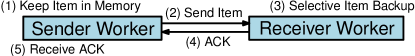
In AF-Stream, item backups are issued by the receiver-side worker (i.e., a downstream worker handles the backups of data and punctuation items, while an upstream worker handles the backups of feedback items). The rationale is that the receiver-side worker can exactly count the number of unprocessed items and decide when to issue item backups. Consider a data item that traverses from an upstream worker to a downstream worker. After the upstream worker sends the data item, it keeps the data item in memory. When the downstream worker receives the data item, it examines the number of unprocessed data items. If the number exceeds the threshold , then the worker makes backups for all pending data items before dispatching the data item to the compute threads for processing. It also returns an acknowledgement (ACK) to the upstream worker, which can then release the cached data item from memory.
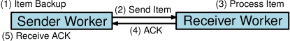
Performing item backups on the receiver side enables us to handle ACKs differently from the traditional upstream backup approach [5, 42, 61], as shown in Figure 3. Upstream backup makes item backups on the sender side. For example, an upstream worker is responsible for making item backups for data items. It caches the output items in memory and waits until its downstream worker replies an ACK. However, the downstream worker sends the ACK only when the item is completely processed, and the upstream worker may need to cache the item for a long time. In contrast, our receiver-side backup approach can send an ACK before an item is processed, and hence limits the caching time in the upstream worker.
We emphasize that our receiver-side backup approach should be viewed as a complementary solution (rather than a replacement) to upstream backup from the perspective of approximate fault tolerance. It still caches items in memory in the upstream worker (as shown in Figure 3(b)) as in upstream backup, but opts to issue backups on the receiver side rather than on the sender side. As discussed above, it not only reduces the caching time in the upstream worker, but also favors our approximate fault tolerance design as the receiver-side worker can count the number of unprocessed data items and issue item backups if the number exceeds the threshold .
(a) Upstream backup
(b) Our receiver-side backup
The rate of item backups in AF-Stream is responsive to the current load of a worker. Specifically, when a worker is heavily loaded, it will accumulate more unprocessed items and hence trigger more backups. Nevertheless, the backup overhead remains limited since item processing is the bottleneck in this case. On the other hand, when a worker is lightly loaded, it issues fewer backups and avoids compromising the processing performance.
Note that the sender-side worker may miss all unacknowledged items if it fails. Currently AF-Stream does not make backups for such unacknowledged items, but instead bounds the maximum number of unacknowledged items (denoted by ) that a worker can cache in memory. If the number of unacknowledged items reaches , then the worker is blocked from sending new items until the number drops. The value of can be generally very small as our receiver-side approach allows a worker to reply an ACK immediately upon receiving an item.
3.4.3 Recovery
If the controller detects a failed worker, it activates recovery and restores the state of the failed worker in a new worker. The new worker calls RecoverState to retrieve the most recent backup state. Also, AF-Stream replays the backup items into the new worker, which can then process them to update the restored state.
Some backup items may have already been processed and updated in the recovered state, and we should avoid the duplicate processing of those items. AF-Stream uses the sequence number information for backup and recovery. When a worker receives an item, it associates the item with a sequence number. Each state also keeps the sequence number of the latest item that it includes. When AF-Stream replays backup items during recovery, it only chooses the items whose sequence numbers are larger than the sequence number kept in the restored state. To reduce the recovery time, our current implementation restores fewer items by replaying only the most recent sequence of consecutive items. Since the number of unprocessed items before the replayed sequence is at most , the errors are still bounded.
3.4.4 User-Configurable Thresholds
AF-Stream exports three user-configurable threshold parameters: (i) , the maximum divergence between the current state and the most recent backup state, (ii) , the maximum number of unprocessed non-backup items and (iii) , the maximum number of unacknowledged items. It automatically tunes the thresholds , , and at runtime with respect to , and , respectively, such that the errors are bounded independent of the number of failures that have occurred and the number of workers in a distributed environment.
How the error bounds quantify the accuracy of a streaming algorithm is specific to the algorithmic design and cannot be directly generalized for all streaming algorithms. Nevertheless, in Appendix A, we present both theoretical analysis and numerical examples on how these parameters are translated to the accuracy of two streaming algorithms, namely heavy-hitter detection in Count-Min Sketch [24] and Ripple Join [32], and show how their accuracy will be degraded under approximate fault tolerance with respect to , , and . Furthermore, in §4, we formally analyze how these parameters affect the model convergence of online learning. We also resort to experiments to empirically evaluate the accuracy for various parameter choices in AF-Stream (§6).
AF-Stream currently requires users to have domain knowledge on configuring the parameters with respect to the desired level of accuracy. We pose the issue of configuring the parameters without user intervention as future work.
3.5 Error Analysis
We analyze how AF-Stream bounds the errors upon failures for different failure scenarios in a distributed environment. We quantify the error bounds in two aspects: (i) the divergence between the actual and ideal states and (ii) the number of lost output items, based on our assumptions (§3.1). In particular, we assume that each lost item brings limited accuracy degradations. To quantify the degradations, after updating the current state with an item, we let the divergence between the current state and the most recent backup state increase by at most and the number of output items generated by the update be at most , where and are two constants specific for a streaming algorithm. Note that both and are introduced purely for our analysis, while programmers only need to configure , , and for building a streaming algorithm. Also, our analysis does not assume any probability distribution of failure occurrences.
3.5.1 Single Failure of a Worker
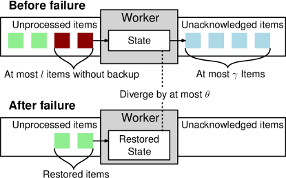
Suppose that AF-Stream sees only a single failure of a worker over its lifetime. We consider the worst case when the failed worker is restored, as shown in Figure 4. First, for the divergence between the actual and ideal states, the restored state diverges from the actual state before the failure by at most , and each of the lost unprocessed items (with at most) changes the divergence by at most . Thus, the total divergence between the actual and ideal states is at most , which is bounded. Second, for the number of lost output items, AF-Stream loses at most unacknowledged output items, and each of the lost unprocessed items (with at most) leads to at most lost output items. Thus, the total number of lost output items is at most , which is also bounded. By initializing , , and as , , and , respectively, we can bound the errors with respect to the user-configurable thresholds.
3.5.2 Multiple Failures of a Single Worker
Suppose that AF-Stream sees multiple failures of a single worker over its lifetime, while other workers do not fail. In this case, the errors after each failure recovery will be accumulated. AF-Stream bounds the accumulated errors by adapting the three thresholds , , and with respect to the three user-configurable parameters , and , respectively, and the number of failures denoted by . First, a worker initializes the thresholds with , , and . After each failure recovery, the worker halves each threshold; in other words, after recovering from failures, the thresholds become , , and . By summing up the errors accumulated over failures, we can show that the divergence between the actual and ideal states is at most and the number of lost output items is at most . Note that the errors are bounded independent of the number of failures .
Our adaptations imply that the thresholds become very small after many failures, so AF-Stream reduces to error-free fault tolerance and makes frequent backups. AF-Stream addresses this issue by allowing the thresholds to be reset. In particular, many streaming algorithms work with windowing, and AF-Stream can use different strategies to reset the thresholds for different windowing types (§3.3). For example, for the hopping window, AF-Stream resets the thresholds to the initial values , , and at the end of a window; for the sliding window, AF-Stream tracks the time of the last failure and increases the thresholds once a failure is not included in the window; for the decaying window, AF-Stream always keeps , , and and disables threshold adaptations, as the errors fade over time.
3.5.3 Failures in Multiple Workers
We address the general case when a general number of failures can happen in multiple workers in a distributed environment. To make the error bounds independent of the number of workers, AF-Stream employs small initial thresholds, such that the accumulated errors are the same as those in the single-worker scenario. Specifically, for operator duplication with copies, AF-Stream initializes each copy with , , and ; for a pipeline with operators, AF-Stream initializes the -th operator in the pipeline with , , and (since each lost item can lead to at most lost output items after pipeline stages). By summing the errors over all failures and all workers, we can obtain the same error bounds as in §3.5.2.
4 Case Study: Convergence of Online Learning
In this section, we analyze how AF-Stream affects the model convergence of online learning.
Our insight is that general machine learning algorithms are known to be iterative-convergent and error-tolerant [14, 25], meaning that they still converge to an optimum even in the face of state errors and loss of items. Offline parameter server systems [25, 35, 47] have leveraged this nature and proposed relaxed consistency models to improve machine learning performance. Here, we prove that AF-Stream preserves the iterative-convergent and error-tolerant nature of online learning independent of the number of failures (defined in §3.5.2).
We focus on online learning algorithms based on stochastic gradient descent (SGD) [12], which has been used by many popular machine learning algorithms to learn model parameters via stochastic optimization [13]. Our goal is to prove that upon the recovery of multiple failures, online learning algorithms based on SGD still converge to an optimum under AF-Stream.
Note that our analysis inherently differs from the standard SGD analysis, as we must address the complicated interactions of SGD and the approximate fault tolerance design of AF-Stream. In particular, after each failure recovery, AF-Stream will (slightly) deviate SGD from its standard behavior, and characterizing the aggregated impact of approximate fault tolerance after multiple failures is non-trivial.
We formulate our analysis as follows. SGD maintains its state as a vector of model parameters. Let denote the state vector of SGD after the -th item is processed, assuming that no failure happens. SGD defines a risk function with respect to the state for each . To update model parameters, SGD first computes the gradient of , followed by updating the vector of model parameters , where is a parameter that controls the learning rate.
The convergence theory of SGD [46, 83] further defines the average risk function (also known as regret) of the first items as . The theory addresses the problem whether the regret can be minimized. Prior studies [25, 35, 46] prove that under certain conditions the regret converges to the global optimum (denoted by ):
We denote the actual model parameters by , as opposed to ideal model parameters denoted by . We also denote the global optimum by . Let be the number of failures encountered by AF-Stream throughout its lifetime. In practice, we expect that is much less than (i.e., the number of items being processed), since failures are less common compared to the numerous items in stream processing. Upon detecting each failure, AF-Stream performs recovery (§3.4.3). Theorem 1 formalizes the convergence guarantee.
Theorem 1.
Consider an SGD sequence generated under AF-Stream. The limit
still holds even after the recovery of failures, provided that .
Proof. See Appendix B.
Remarks.
5 Implementation
We have implemented a prototype of AF-Stream in C++. AF-Stream connects the controller and all workers using ZooKeeper [40] to manage fault tolerance. It also includes a backup server, which is now implemented as a daemon that receives backup states and items from the workers via TCP and writes them to its local disk. Our current prototype has around 47,800 LOC in total.
Our prototype realizes a number of built-in primitive operators and their implementations of StateDivergence, BackupState, and RecoverState, listed in Appendix C. We now support the numeric variable, vector, matrix, hash table, and set, and provide them with built-in fault tolerance. For example, we can keep elements in our built-in hash table, whose fault tolerance is automatically enabled. Programmers can also build their own fault-tolerant operators via implementing the above three interfaces.
While we currently implement AF-Stream as a clean-slate system, we explore how to integrate our approximate fault tolerance notion into existing stream processing systems in future work. Such integration must address at least the following technical challenges, including: (i) the three interfaces (i.e., StateDivergence, BackupState, and RecoverState) for state backup (§3.4.1), (ii) the receiver-side backup and acknowledgement mechanisms for item backup (§3.4.2), (iii) the new recovery mechanism (§3.4.3), and (iv) the user-configurable thresholds (§3.4.4).
Communication optimization.
Our prototype specifically optimizes both inter-thread and inter-worker communications for high-throughput stream processing. For inter-thread communications, we implement a lock-free multi-producer, single-consumer (MPSC) ring buffer [56]. We assign one MPSC ring buffer per destination, and group output items from different compute threads by destinations (§3.2). This offloads output item scheduling to compute threads, and simplifies subsequent inter-worker communications. Also, we only pass the pointers to the items to the ring buffer, so that the rate of the number of items that can be shared is independent of the item size.
For inter-worker communications, we implement a bi-directional network queue with ZeroMQ [82]. ZeroMQ itself uses multiple threads to manage TCP connections and buffers, and the thread synchronization is expensive. Thus, we modify ZeroMQ to remove its thread layer, and make the upstream and downstream threads of a worker directly manage TCP connections and buffers. The modifications enable us to achieve high-throughput stream processing in a 10 Gb/s network (§6).
Asynchronous backups.
We further mitigate the performance degradation of making backups using an asynchronous technique similar to [30]. Specifically, our prototype employs a dedicated backup thread for each worker. It collects all backups of a worker and sends them to the backup server, allowing other threads to proceed normal processing after generating backups. Note that the asynchronous technique does not entirely eliminate backup overhead, since the backup thread can still be overloaded by frequent backup operations. Thus, we propose approximate fault tolerance to limit the number of backup operations.
Consistency models.
AF-Stream currently supports different consistency models to synchronize the views of workers. For example, in SGD, AF-Stream processes streaming items in multiple local workers, each of which computes gradients on the items based on its local model and sends the local gradient results to a global worker. The global worker aggregates all the results to update its global model, and feedbacks the updated global model to each local worker to update its local model. AF-Stream can choose one of the following three consistency models for synchronizing the model updates: (i) the Asynchronous Parallel (ASP) model [84], in which after a local worker sends local results to the global worker, it continues to use its (stale) local model to compute gradients for the new incoming items, until the global worker feedbacks an updated global model; (ii) the Bulk Synchronous Parallel (BSP) model [15], in which after a local worker sends local results to the global worker, it stops working and waits until receiving the feedback from the global worker; and (iii) the Stale Synchronous Parallel (SSP) model [35], which allows local workers to use the stale model with at most an additional number of iterations (which is user-configurable). Note that the BSP model is adopted by Spark Streaming [80], which processes streaming items in mini-batches.
6 Experiments
We present evaluation results on AF-Stream through experiments on Amazon EC2 and a local cluster.
| Algorithm | Upstream stage | Downstream stage | State | Trace | ||
| (# workers) | (# workers) | (Divergence) | Source | # items | Size | |
| Grep | Parse and send the lines with the matched pattern (10) | Merge matched lines (1) | None | Gutenberg [59] | 300M | 15 GB |
| WordCount | Parse and send words with intermediate counts (4) | Aggregate intermediate word counts (7) | Hash table of word counts (maximum difference of word counts) | Gutenberg [59] | 300M | 15 GB |
| HH detection | Update packet headers into a local sketch and send the local sketch and local HHs (10) | Merge local sketches into a global sketch, and check if local HHs are actual HHs with the global sketch (1) | Matrix of counters (maximum difference of counter values in bytes) | Caida [17] | 1G | 40 GB |
| Online join | Find and send tuples that have matching packet headers in two streams (2) | Perform join and aggregation (9) | Set of sampled items (difference of number of packets) | Caida [17] | 1G | 40 GB |
| Online logistic regression | Train and send the local model, and update the local model with feedback items (10) | Merge local models to form a global model, and send the global model as feedback items (1) | Hash table of model parameters (Euclidean distance) | KDD Cup 2012 [58] | 110M | 42 GB |
6.1 Performance on Amazon EC2
We first evaluate AF-Stream on an Amazon EC2 cluster. The cluster is located in the us-east-1b zone. It comprises a total of 12 instances: one m4.xlarge instance with four CPU cores and 16 GB RAM, and 11 c3.8xlarge instances with 32 CPU cores and 60 GB RAM each. We deploy the controller and the backup server in the m4.xlarge instance, and a worker in each of the c3.8xlarge instances. We connect all instances via a 10 Gb/s network.
Our experiments consider five streaming algorithms: Grep, WordCount, heavy hitter detection, online join, and online logistic regression. The latter three algorithms are chosen as the representatives for data synopsis, stream database queries, and online learning, respectively (§2.2). We pipeline each streaming algorithm in two stages, in which the upstream stage reads traces, processes items, and sends intermediate outputs to the downstream stage for further processing. Each stage contains one or multiple workers. We evenly partition a trace into subsets and assign each subset to an upstream worker, which partitions its intermediate outputs to different downstream workers if more than one downstream worker is used. Table 3 summarizes each algorithm, including the functionalities and number of workers for both upstream and downstream stages, the definitions of the state and the corresponding state divergence, as well as the source, number of items, and size of each trace. We elaborate the algorithm details later when we present the results.
Each experiment shows the average results over 20 runs. Before each measurement, we load traces into the RAM of each upstream worker, which then reads the traces from RAM during processing. This eliminates the overhead of reading on-disk traces, and moves the bottleneck to AF-Stream itself.
We evaluate the throughput and accuracy of AF-Stream for each algorithm, and show the trade-off with respect to , , and . For throughput, we measure the rate of the amount of data processed in each upstream worker, and compute the sum of rates in all upstream workers as the resulting throughput. For accuracy, we provide the specific definition for each algorithm when we present the results.
6.1.1 Baseline Performance
We benchmark the baseline performance of AF-Stream using two algorithms: Grep, which returns the input lines that match a pattern, and WordCount, which counts the occurrence frequency of each word. Note that Grep does not need any state to be kept in a worker, while WordCount defines a state as a hash table of word counts. We implement both algorithms based on their implementations in open-source Spark Streaming [80]. We use the documents on Gutenberg [59] as the inputs, with the total size 15 GB.
Experiment 1 (Comparisons with existing fault tolerance approaches).
We compare AF-Stream with two open-source stream processing systems: Storm (v0.9.5) [69] and Spark Streaming (v1.4.1) [80]. We consider three setups for each of them. The first setup disables fault tolerance to provide baseline results. The second setup uses their own available fault tolerance mechanisms. Specifically, Storm tracks every item until it is fully processed (via a component called Acker), yet it only achieves best-effort fault tolerance as it does not support state backups. On the other hand, Spark Streaming achieves error-free fault tolerance by making state backups as RDDs in mini-batches and making item backups via write-ahead logging [81]. We set the mini-batch interval of Spark Streaming as 1s (§2.1). For both setups, we configure the systems to read traces from memory to avoid the disk access overhead. Finally, the third setup achieves fault tolerance through Kafka [7], a reliable messaging system that persists items to disk for availability. We configure the systems to read input items from the disk-based storage of Kafka, so that Kafka serves as an extra item backup system to replay items upon failures. We configure the fault tolerance mechanisms of Storm and Spark Streaming based on the official documentations; for Kafka integration, we refer to [68, 70]. In particular, Kafka and write-ahead logging in Spark Streaming have the same functionality, so for performance efficiency, it is suggested to disable write-ahead logging when Kafka is used [68]. On the other hand, other fault tolerance approaches can be used in conjunction with Kafka. We present all combinations in our results.
In addition, we implement existing fault tolerance approaches in AF-Stream and compare them with approximate fault tolerance under the same implementation setting. We consider mini-batch and upstream backup. Mini-batch follows Spark Streaming [80] and makes backups for mini-batches. To realize the mini-batch approach in AF-Stream, we divide a stream into mini-batches with the same number of items, such that the number of items per mini-batch is the maximum number while keeping the system stable (§2.1). Our approach generates around 800 mini-batches. Our modified AF-Stream then issues state and item backups for each mini-batch. On the other hand, upstream backup [41] provides error-free fault tolerance by making backups in upstream workers. To realize upstream backup, we issue a backup for every data item, while we issue a state backup every 1% of data items. In addition to saving items via the backup server, both approaches also keep the items in memory for ACKs. Once the memory usage exceeds a threshold (1 GB in our case), we save any new item to local disk. Finally, we set , , and in AF-Stream for approximate fault tolerance.
| Grep | WordCount | |
| Storm | ||
| No fault tolerance | 262.04 MB/s | 901.47 MB/s |
| With item backup only | 100.65 MB/s | 571.31 MB/s |
| With Kafka only | 85.79 MB/s | 192.66 MB/s |
| With Kafka + item backup | 80.14 MB/s | 174.30 MB/s |
| Spark Streaming | ||
| No fault tolerance | 178.61 MB/s | 754.02 MB/s |
| With RDD + write-ahead logging | 93.61 MB/s | 466.07 MB/s |
| With Kafka only | 81.49 MB/s | 147.28 MB/s |
| With Kafka + RDD | 75.09 MB/s | 140.80 MB/s |
| AF-Stream implementation | ||
| No fault tolerance | 3.55 GB/s | 1.92 GB/s |
| Mini-batch | 358.16 MB/s | 380.49 MB/s |
| Upstream backup | 379.61 MB/s | 373.89 MB/s |
| Approximate fault tolerance | 3.48 GB/s | 1.88 GB/s |
Table 4 shows the throughput of different fault tolerance approaches. Both Storm and Spark Streaming see throughput drops when fault tolerance is used. Compared to the throughput without fault tolerance, even the most modest case degrades the throughput by around 37% (i.e., Storm’s item backup for Grep). We find that the bottlenecks of both systems are mainly due to frequent item backups. Also, Kafka integration achieves even lower throughput since Kafka incurs extra I/Os to read traces from disk. In contrast, AF-Stream with approximate fault tolerance issues fewer backup operations. It achieves 3.48 GB/s for Grep and 1.78 GB/s for WordCount, both of which are close to when AF-Stream disables fault tolerance. Note that AF-Stream outperforms Spark Streaming and Storm even when they disable fault tolerance. The reason is that AF-Stream has a more simplified implementation.
Experiment 2 (Impact of thresholds on performance).
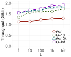
We examine how the thresholds , , and affect the performance of AF-Stream in different aspects. Since Grep does not keep any state, we focus on WordCount. We vary and , and fix . When and are sufficiently large (i.e., close to infinity), we in essence disable both state and item backups, respectively.
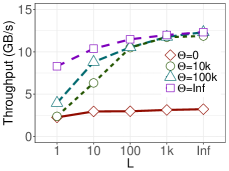
Figure 5(a) presents the throughput of AF-Stream versus for different settings of and the case of disabling state backups. Compared to disabling state backups, the throughput loss is 33% when , but we reduce the loss to 10% by setting .
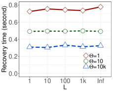
Figure 5(b) also presents the recovery time when recovering a worker failure, starting from the time when a new worker process is resumed until it starts normal processing. A smaller implies a longer recovery time, as we need to make backups for more updated state values in partial backup (§3.4.1). Nevertheless, the recovery time in all cases is less than one second.
 |
 |
| (a) Throughput | (b) Recovery time |
 |
 |
| (c) Fraction of state backups | (d) Fraction of item backups |
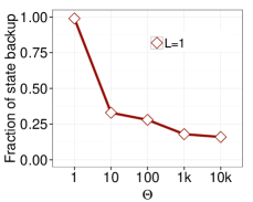
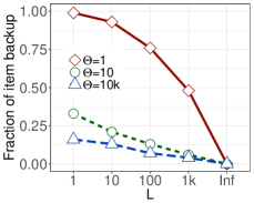
We justify our throughput results by showing the fractions of state and item backup operations over the total number of items. Figure 5(c) shows that AF-Stream issues state backups for less than 30% of items when (where we fix ). Figure 5(d) shows that increasing also reduces the fraction of item backups (e.g., to less than 20% when ), mainly because the compute threads have more available resources to process items rather than perform state backups. This reduces the number of unprocessed items, thereby issuing fewer item backups.
6.1.2 Performance-accuracy Trade-offs
We examine how AF-Stream trades between performance and accuracy. We evaluate its throughput when no failure happens, while we evaluate its accuracy after recovering from system failures in which all workers fail. To mimic a system failure, we inject a special item in the stream to a worker. When the worker reads the special item, it sends a remote stop signal to kill all worker processes. We then resume all worker processes, recover all backup states, and replay the backup items. We inject the special item multiple times to generate multiple failures over the entire stream. We consider the other three streaming algorithms, which are more complicated than Grep and WordCount.
In the following, we vary and , and fix . Here, represents the maximum number of unacknowledged items in upstream workers. We observe that the actual number of unacknowledged items is small and they have limited impact on both performance and accuracy in our experiments. Thus, we focus on the physical meanings of and in each algorithm and justify our choices of the two parameters.
 |
 |
| (a) Throughput | (b) Precision |
Experiment 3 (Heavy hitter detection).
We perform heavy hitter (HH) detection in a stream of packet headers from CAIDA [17], where the total packet header size is 40 GB. We define an HH as a source-destination IP address pair whose total payload size exceeds 10 MB. We implement HH detection based on Count-Min Sketch [24]. Each worker holds a Count-Min Sketch with four rows of 8,000 counters each as its state. Each packet increments one counter per row by its payload size. We maintain the counters in a matrix that has built-in fault tolerance (§5). Also, an upstream worker sends local sketches and detection results to a downstream worker as punctuation items, for which we ensure error-free fault tolerance (§3.4.2).
In our implementation, is the maximum difference of counter values (in bytes) between the current state and the most recent backup state and is the maximum number of unprocessed non-backup packets. We choose and . If the packet size is at most 1,500 bytes, our choices account for at most 1.5 MB of counter values, much smaller than our selected threshold 10 MB.
We measure the throughput of AF-Stream as the total packet header size processed per second. To measure the accuracy, one important fix is that we need to address the missing updates due to approximate fault tolerance. In particular, the missing updates cause the restored counter values to be smaller than the original counter values before a failure. To compensate for the missing updates, we add each counter by when restoring counter values after the -th failure (where ). This ensures the zero false negative rate of Count-Min Sketch, while increasing the false positive rate by a bounded value. We measure the accuracy by the precision, defined as the ratio of the number of actual HHs to the number of returned HHs (which include false positives).
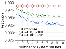
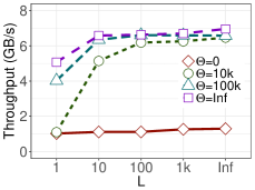
Figure 6 presents the throughput and precision of AF-Stream for HH detection. If we disable both state and item backups (i.e., and are close to infinity), the throughput is 12.33 GB/s, and the precision is 98.9% when there is no failure. With approximate fault tolerance, if and , the throughput decreases by up to 4.7%, yet the precision only decreases to 92.8% after 10 system failures. If we set and , the throughput drops by around 15%, while the precision decreases to 95.5%.
Experiment 4 (Online join).
Online join is a basic operation in stream database queries. This experiment considers an online join operation that correlates two streams of packet headers of different cities obtained from CAIDA [17], with the total packet header size 40 GB. Our goal is to return the tuples of the destination IP address and timestamp (in units of seconds) that have matching packet headers in both streams, meaning that both streams visit the same host at about the same time. We partition the join operator into multiple workers, each of which runs a Ripple Join algorithm [32] to sample a subset of packets for online join at a sampling rate 10%. Each worker keeps the sampled packets in a set with built-in fault tolerance (§5).
Here, represents the maximum difference of the numbers of packets between the current state and the most recent backup state, and is the maximum numbers of unprocessed non-backup packets. We find that our sampling rate can obtain around 100 million packets. Thus, we set and to account for at most 0.1% of sampled packets.
We again measure the throughput of AF-Stream as the total packet header size processed per second. To measure the accuracy, we issue an aggregation query for the total number of joined tuples. Ripple join returns the estimated number of tuples by dividing the number of joined tuples in the sampled set by the sampling rate. We measure the accuracy as the relative estimation error, defined as the percentage difference of the estimated number from the actual number without any sampling.
Figure 7 presents the throughput and relative estimation error of AF-Stream for online join. If we disable both state and item backups, the throughput is 6.96 GB/s. The relative estimation error is 9.1% when no failure happens. If we enable approximate fault tolerance, the throughput drops by 5.2% for and , and by 12% for and , while the relative estimation error only increases to 11.3% and 10.6%, respectively, even after 10 system failures.
 |
 |
| (a) Throughput | (b) Relative estimate error |
Experiment 5 (Online logistic regression).
Logistic regression is a classical algorithm in machine learning. We use online logistic regression to predict advertisement click-through rates for a public trace in KDD Cup 2012 [58]. We extract a trace with 150 million tuples, each of which is associated with a label and multiple features. However, we find that 40 million of them have a missing value in one of the features. We remove these 40 million anomalous tuples from the trace and use the remaining 110 million tuples (with a total size 42 GB) in our evaluation; nevertheless, we include those anomalous tuples in our convergence evaluation to show the robustness of AF-Stream in model training (§6.2).
We evenly divide the entire trace into two halves, one as a training set and another as a test set. We train the model with a distributed SGD technique [46], in which each upstream worker trains its local model with a subset of the training set, and regularly sends its local model to a single downstream worker (every tuples in our case) in the form of a punctuation item (§3.4.2). The online logistic regression algorithm has a feedback loop, in which the downstream worker computes the average of the model parameters to form a global model, and sends the global model to each upstream worker in the form of a feedback item. The upstream worker updates its local model accordingly. Each upstream worker stores the model parameters in a hash table as its state. In this experiment, we configure AF-Stream to run in the ASP consistency model (§5).
Here, represents the Euclidean distance of the model parameters, and is the maximum number of unprocessed non-backup tuples for model training. As our model has more than features, we set and to limit the errors to the model parameters. This setting implies an average Euclidean distance of less than for each feature parameter and at most of lost tuples.
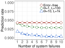
We measure the throughput as the number of tuples processed per second. To measure the accuracy, we predict a label for each tuple in the test set based on its features by logistic regression, and check if the predicted label is identical to the true label associated with the tuple. We measure the accuracy as the prediction rate, defined as the fraction of correctly predicted tuples over all tuples in the test set.
Figure 8 presents the throughput and prediction rate of AF-Stream for online logistic regression. The throughput is 62,000 tuples/s when we disable state backups. If we set and , or and , the throughput is only less than that without state and item backups by up to 0.3%. The reason is that the model has a large size with millions of features and incurs intensive computations. Thus, the throughput drops due to state backups become insignificant. In addition, the prediction rate is 94.3% when there is no failure. The above two settings of and decrease the prediction rate to 90.4% and 92.9%, respectively, after 10 system failures.
 |
 |
| (a) Throughput | (b) Prediction rate |
| HH detection, | Online join, | Online LR, | |
| No fault tolerance | 12.33 GB/s | 6.96 GB/s | 62,699 tuples/s |
| Mini-batch | 0.91 GB/s | 0.89 GB/s | 14,770 tuples/s |
| Upstream backup | 0.89 GB/s | 0.87 GB/s | 12,827 tuples/s |
| Approximate fault tolerance | 11.77 GB/s | 6.59 GB/s | 62,292 tuples/s |
Discussion.
Our results demonstrate how AF-Stream addresses the trade-off between performance and accuracy for different parameter choices. We also implement the three algorithms under existing fault tolerant approaches as in Experiment 1, and Table 5 summarizes the results. We observe that both mini-batch and upstream backup approaches reduce the throughput to less than 25% compared to disabling fault tolerance, while approximate fault tolerance achieves over 95% of the throughput.
6.2 Convergence Evaluation on a Local Cluster
 |
 |
| (a) KDDCup, Spark Streaming | (b) HIGGS, Spark Streaming |
 |
 |
| (c) KDDCup, Flink | (d) HIGGS, Flink |
 |
 |
| (e) KDDCup, AF-Stream | (f) HIGGS, AF-Stream |
 |
 |
| (a) KDDCup, Spark Streaming | (b) HIGGS, Spark Streaming |
 |
 |
| (c) KDDCup, Flink | (d) HIGGS, Flink |
 |
 |
| (e) KDDCup, AF-Stream | (f) HIGGS, AF-Stream |
We further show how AF-Stream preserves the model convergence of online learning with respect to failure patterns, traces, and parameter choices. We conduct our experiments on a local cluster with a total of 12 machines, each equipped with an Intel Core i5-7500 3.40 GHz quad-core CPU, 32 GB RAM, and a TOSHIBA DT01ACA100 7200 RPM 1 TB SATA disk. All machines run Ubuntu 16.04 LTS and are connected via a 10 Gb/s switch.
We focus on the model training of online logistic regression, and compare the convergence performance under AF-Stream with that under Spark Streaming (v1.6.3) [80] and Flink (v1.7.2) [19]; both Spark Streaming and Flink can achieve error-free fault tolerance. Recall that Spark Streaming partitions a stream into mini-batches on small time-steps and issues both state backups as checkpoints and item backups via write-ahead logging, while Flink issues state backups as checkpoints and persists items in Kafka for item backups (§2.1).
We run the model training of online logistic regression on two real-world traces. The first trace, denoted by KDDCup, is the same public trace from KDD Cup 2012 [58] used in Experiment 5 in §6.1. We use all 150 million tuples in the trace, including the 40 million anomalous tuples (§6.1). We preprocess the trace so that each item has 11 features. The second trace, denoted by HIGGS, contains items for the classification of signal and background processes in high-energy physics experiments [9]. Note that we concatenate the original HIGGS trace five times to obtain 55 million items with 28 features each.
For each trace, AF-Stream, Flink, and Spark Streaming train a regression model with SGD; in Spark Streaming, we implement SGD using MLlib [54]. In Flink, since its machine learning library (called FlinkML) only supports batch processing, we re-implement SGD based on the implementation in MLlib. We partition each trace across 11 local workers in 11 different machines, each of which iteratively performs gradient computations and sends the results to a global worker in the remaining machine. We evaluate the performance and accuracy of our model training via three metrics: throughput, convergence time, and the L1-norm difference between the models in the last and current iterations. For AF-Stream, by default, we set , and consider different values of and in our experiments (in Appendix B, we show that the effect of is included in state divergence, which is controlled by ).
Experiment 6 (Impact of fault tolerance on throughput).
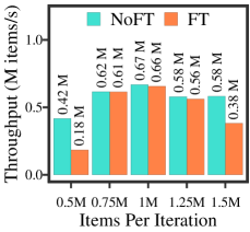
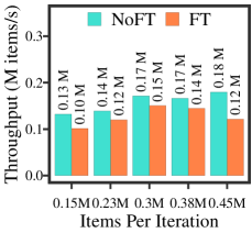
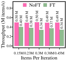
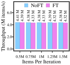
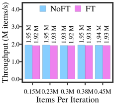
We first examine how fault tolerance mechanisms influence the throughput of model training. For fair comparisons, we configure all systems to operate in the BSP consistency model (§5) and process streaming items in mini-batches, each of which corresponds to an iteration. For Flink, to realize the BSP model, we use its countWindowAll API to aggregate the streaming items in tumbling windows that resemble mini-batches. We set the stream input rates as 0.5 million and 0.15 million items per second for KDDCup and HIGGS, respectively. We vary the iteration size (i.e., the number of items being processed per iteration) in our evaluation. For AF-Stream, we set and vary as 0.1, 1, and 10 and obtain the average results.
Figure 9 compares the throughput with and without fault tolerance versus the iteration size. Recall from Experiment 1 that AF-Stream has high absolute throughput due to a simplified implementation. Thus, our focus here is not to compare the absolute throughput of different systems. Instead, we focus on comparing the performance differences with and without enabling fault tolerance.
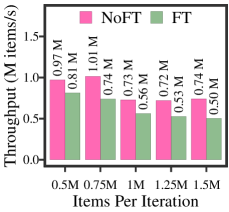
We first consider Spark Streaming. For KDDCup, the fault tolerance overhead in Spark Streaming’s throughput (Figure 9(a)) depends on the iteration size. If the iteration size is 0.5 million items per iteration, enabling fault tolerance drops the throughput by 57%. The reason is that the number of mini-batches over the entire stream becomes high and Spark Streaming needs to trigger a high number of state backups. As the iteration size increases (i.e., the number of mini-batches decreases), the fault tolerance overhead is negligible. However, when the iteration size reaches 1.5 million items per iteration, enabling fault tolerance drops the throughput by 34%, since a worker now needs more resources to process a large number of items in each iteration in time. Spark Streaming shows a similar trend in HIGGS as in KDDCup (Figure 9(b)). When the iteration size is 0.15 million items per iteration, the throughput drops by 23%. The throughput drop reduces to 13% on average when the iteration size increases from 0.23 million to 0.38 million items per iteration, but increases again to 32% when the iteration size reaches 0.45 million items per iteration. We also observe similar results for Flink, in which enabling fault tolerance drops the throughput by 25% and 26% on average in KDDCup and HIGGS, respectively (Figures 9(c) and 9(d)). On the other hand, AF-Stream’s throughput (Figures 9(e) and 9(f)) remains stable for any iteration size in both traces. It drops by only 1.14% and 1.06% on average for KDDCup and HIGGS, respectively, when approximate fault tolerance is used.
 |
 |
| (a) KDDCup, varying , | (b) KDDCup, varying , |
 |
 |
| (c) HIGGS, varying , | (d) HIGGS, varying , |
Experiment 7 (Convergence under failures).
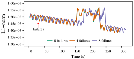
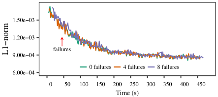
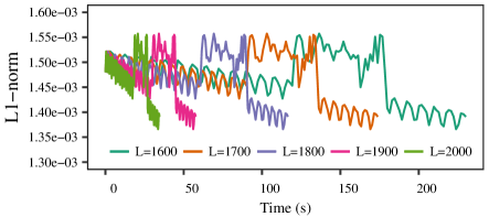
We next evaluate the model convergence time when the systems operate under failures. In all systems, we kill a number of local workers to mimic simultaneous failures after they have processed 10% of all input items. For Spark Streaming, it will recover the lost states and items and re-distribute the workloads to the other non-failed workers. For Flink, when some workers fail, it needs to first stop the whole job, including the processing of other non-failed workers. It then restarts the job from the latest checkpoint. For AF-Stream, we immediately restart the workers at the same machines where they fail. For AF-Stream, we set and . All systems operate under the BSP consistency model. We set the iteration size as 1 million and 0.3 million items per iteration for KDDCup and HIGGS, respectively. We consider the cases when there is no failure and when we issue four or eight failures. Figure 10 shows the results.
First, note that for KDDCup (Figures 10(a), 10(c), and 10(e)), there is a sharp increase in L1-norm even though there is no failure (from time 155s to 229s in Spark Streaming, from time 114s to 168s in Flink, and from time 18s to 26s in AF-Stream). The reason is attributed to the 40 million anomalous tuples with a missing feature in that period. Nevertheless, AF-Stream still ensures that the model converges even under failures as compared to without failures.
Specifically, Spark Streaming provides error-free fault tolerance. For KDDCup (Figure 10(a)), it has the same convergence pattern even with four failures as in the no-failure case. Even when there are eight failures, the convergence time is only slightly delayed, for example, from 297s in the no-failure case to 314s (i.e., 5.7% delay) so as to reach the final L1-norm equal to 1.4e-3. For HIGGS (Figure 10(b)), Spark Streaming has the same convergence pattern with both four and eight failures as in the no-failure case.
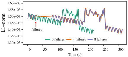
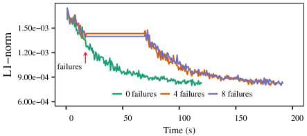
Similarly, Flink sees delayed convergence under failures (Figures 10(c) and 10(d)). In particular, it takes more than 50s to restart the whole job when failures happen. Thus, with eight failures, the convergence time increases from 218s in the no-failure case to 313s to reach the final L1-norm 1.4e-3 in KDDCup, and from 120s in the no-failure case to 191s to reach the final L1-norm 8e-4 in HIGGS.
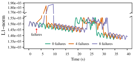
AF-Stream has a different convergence pattern when failures happen. For KDDCup (Figure 10(e)), the L1-norm sharply increases right after the failures are issued and recovered, since AF-Stream incurs errors in gradient computation upon the recovery of failures. Nevertheless, the errors are amortized after processing six and ten iterations for four and eight failures, respectively. The model converges slightly later than the no-failure case, as AF-Stream issues more backups before the errors are amortized. For example, in the no-failure case, the model takes 35.4s to converge to the final L1-norm equal to 1.4e-3; where there are four and eight failures, the convergence time slightly increases to 38.1s (i.e., 7.6% delay) and 40.1s (i.e., 13.3% delay), respectively. For HIGGS (Figure 10(f)), the L1-norm does not significantly change right after the failures are issued and recovered, yet these failures delay the convergence as they trigger more backups in AF-Stream as in KDDCup. With four and eight failures, the convergence time slightly increases from 28.2s to 31.7s (i.e., 12.4% delay) and 33.9s (i.e., 20% delay), respectively, to reach the final L1-norm 8e-4.
 |
 |
| (a) KDDCup | (b) HIGGS |
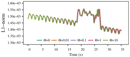
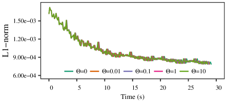
Experiment 8 (Impact of parameters on the model convergence of AF-Stream).
We evaluate how various parameters affect the model convergence of AF-Stream. We focus on studying and , as they affect the convergence performance as shown in the proof of Theorem 1 (Appendix B). We set the iteration size as 1 million and 0.3 million items per second for KDDCup and HIGGS, respectively, and run AF-Stream under the BSP consistency model.
We first study KDDCup. Figure 11(a) shows the model convergence of AF-Stream for different values of for KDDCup, where we fix . If we use smaller , the model convergence time significantly increases. The reason is that AF-Stream now issues more item backups to satisfy the fault tolerance requirement, and such backup overhead significantly degrades the overall performance. Note that increasing beyond 2000 has roughly the same performance as in , so we only show the results of up to 2000 for brevity. Figure 11(b) shows the model convergence of AF-Stream for different values of , where we fix . The model convergence time remains fairly the same. It shows that the impact of is much greater than that of . We also show the impact of parameters for HIGGS (Figures 11(c) and 11(d)), and the observations are similar.
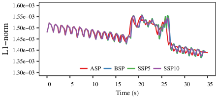
Experiment 9 (Consistency models).
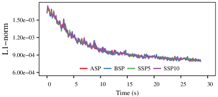
We further study how AF-Stream performs under different consistency models (i.e., ASP, BSP, and SSP); for SSP, we configure each local worker to use the stale model for at most five and ten additional iterations (denoted by SSP-5 and SSP-10, respectively). We set the iteration size as 1 million and 0.3 million items for KDDCup and HIGGS, respectively. We also set and .
Figure 12 shows the results. We find that the model convergence performance is highly similar across different consistency models in both traces. In all cases, the models converge to the same final L1-norm. This demonstrates that AF-Stream works well with different consistency models. In particular, as all local workers have similar processing speeds, we do not see significant performance differences between BSP and ASP, even though all local workers need to wait until receiving the feedback from the global worker in each iteration under BSP (§5).
Discussion.
Our results show that AF-Stream preserves the iterative-convergent and error-tolerant nature of online learning based on stochastic gradient descent, which also validates the conclusion of our theoretical analysis. In particular, AF-Stream maintains the model convergence of online logistic regression in the presence of failures, and the convergence still holds for different traces and parameter settings.
7 Related Work
Best-effort fault tolerance. Some stream processing systems only provide best-effort fault tolerance. They either discard missing items (e.g., [57]) or missing states (e.g., [6, 69, 45]), or simply monitor data loss and return the data completeness to developers (e.g., [43, 51]). These systems may have unbounded errors in the face of failures, making the processing results useless. In contrast, AF-Stream bounds errors upon failures with theoretical guarantees.
Error-free fault tolerance.
Early stream processing systems extend traditional relational databases to distributed stream databases to support SQL-like queries on continuous data streams. They support error-free fault tolerance, and often adopt active standby (e.g., [64, 8]) or passive standby (e.g., [20, 41, 42, 44]). Active standby employs backup nodes to execute the same computations as primary nodes, while passive standby makes periodic backups for states and items to backup nodes. Both approaches, however, are expensive due to maintaining redundant resources (for active standby) or issuing frequent backup operations (for passive standby).
Some stream processing systems realize upstream backup, in which an upstream worker keeps the items that are being processed in its downstream workers until all downstream workers acknowledge the completion of the processing. The upstream worker replays the kept items when failures happen. This approach is used extensively by previous studies [5, 61, 29, 75, 55, 38, 49, 74]. Upstream backup generally incurs significant overhead to normal processing, as a system needs to save a large number of items for possible replays (§3.4.2).
To mitigate the impact on normal processing, asynchronous state checkpoints [53, 30] allow normal processing to be performed in parallel with state backups. However, they are not designed for stream processing and do not address item backups, which could be expensive. StreamScope [48] provides an abstraction to handle failure recovery, but does not address how to trade between performance and accuracy in fault tolerance as in AF-Stream.
Incremental processing.
Incremental processing systems extend batch processing systems for stream processing, by incrementally batching processing at small timescales. Some systems extend MapReduce [27] by pipelining mapper and reducer tasks (e.g., [21]), while others explicitly divide a stream into mini-batches and run batch-based processing for each mini-batch (e.g., [50, 34, 11, 80]). Incremental processing systems inherently support error-free fault tolerance because all data is available to regenerate states upon failures, but they incur high I/O overhead in saving all items for availability.
Approximation techniques.
Recent distributed systems have extensively adopted approximation techniques to improve performance. For example, BlinkDB [2] is a database which samples a subset of data to reduce query latency. Some machine learning systems (e.g., [47, 76, 77]) defer synchronization to reduce communication costs. In the context of stream processing, JetStream [63] deploys tunable operators that automatically trade accuracy for bandwidth saving in wide-area stream processing. Approximate Spark Streaming [3] samples a subset of items in continuous streams for actual processing. AF-Stream differs from them by leveraging approximations in fault tolerance for distributed stream processing.
Load shedding [71, 72] is a technique that enables an overloaded stream processing system to drop unprocessed streaming items, with a trade-off of producing approximate outputs. Both load shedding and AF-Stream target different reliability aspects in stream processing: (i) load shedding addresses system overloading, while AF-Stream focuses on fault tolerance; (ii) load shedding is activated upon system overloading, while AF-Stream proactively mitigates backup overhead and provides error bounds in failure recovery; and (iii) load shedding does not mitigate overhead due to state backup. Nevertheless, AF-Stream can also be integrated with load shedding to address overloading conditions.
LAAR [10] supports adaptive replication by dynamically activating or deactivating replication for processing elements based on the service-level agreement requirements, so as to improve processing capacities. AF-Stream targets the adaptive backups for internal states and streaming items, and we provide error bounds independent of the number of failures.
Zorro [60] introduces approximation techniques to handle failures in graph processing. It exploits vertex replication in distributed graph processing to reconstruct lost states with a high probability. While the idea is similar to approximate fault tolerance, it is not applicable for stream processing since streaming items do not exhibit such replication nature.
Convergence of online learning.
The convergence property of online learning has been well studied and analyzed through game theory [33] or stochastic programming [14]. Many follow-up studies extend the convergence analysis of online learning for different settings, such as signal processing paradigms [16], delayed updates in parallel computing architectures [46], and platforms with adversarial delays [62]. In contrast to the current studies, we analyze the convergence of online learning in distributed stream processing under approximate fault tolerance.
8 Conclusions
We propose AF-Stream, a distributed stream processing system that realizes approximate fault tolerance for both internal states and unprocessed items. AF-Stream achieves not only high performance by reducing the number of backup operations, but also high accuracy by bounding errors upon failures with theoretical guarantees. It provides an extensible programming model and exports user-configurable threshold parameters for configuring the performance-accuracy trade-off. In addition, it provably preserves the iterative-convergent and error-tolerant nature of online learning based on SGD. Experiments on our AF-Stream prototype demonstrate its high performance and high accuracy in various streaming algorithms, as well as its model convergence in various settings.
References
- [1] D. J. Abadi, D. Carney, U. Cetintemel, M. Cherniack, C. Convey, S. Lee, M. Stonebraker, N. Tatbul, and S. Zdonik. Aurora: A New Model and Architecture for Data Stream Management. The VLDB Journal, 12:120–139, 2003.
- [2] S. Agarwal, B. Mozafari, A. Panda, H. Milner, S. Madden, and I. Stoica. BlinkDB: Queries with Bounded Errors and Bounded Response Times on Very Large Data. In Proc. of EuroSys, pages 29–42, 2013.
- [3] S. Agarwal and K. Zeng. BlinkDB and G-OLA: Supporting Continuous Answers with Error Bars in SparkSQL. In Spark Summit, 2015.
- [4] A. Ahmed, M. Aly, J. Gonzalez, S. Narayanamurthy, and A. J. Smola. Scalable Inference in Latent Variable Models. In Proc. of WSDM, 2012.
- [5] T. Akidau, A. Balikov, K. Bekiro, S. Chernyak, J. Haberman, R. Lax, S. Mcveety, D. Mills, P. Nordstrom, and S. Whittle. MillWheel: Fault-Tolerant Stream Processing at Internet Scale. In Proc. of VLDB Endowment, volume 6, pages 1033–1044, 2013.
- [6] Apache Flume. http://flume.apache.org.
- [7] Apache Kafka. http://kafka.apache.org.
- [8] M. Balazinska, H. Balakrishnan, S. R. Madden, and M. Stonebraker. Fault-Tolerance in the Borealis Distributed Stream Processing System. In Proc. of SIGMOD, pages 13–24, 2005.
- [9] P. Baldi, P. Sadowski, and D. Whiteson. Searching for Exotic Particles in High-energy Physics with Deep Learning. Nature communications, 2014.
- [10] P. Bellavista, A. Corradi, S. Kotoulas, and A. Reale. Adaptive Fault-Tolerance for Dynamic Resource Provisioning in Distributed Stream Processing Systems. In Proc. of IEEE EDBT, pages 85–96, 2014.
- [11] P. Bhatotia, A. Wieder, R. Rodrigues, U. Acar, and R. Pasquin. Incoop: Mapreduce for Incremental Computations. In Proc. of SoCC, pages 7:1–7:14, 2011.
- [12] L. Bottou. Online Algorithms and Stochastic Approximations. In Online Learning and Neural Networks, 1998.
- [13] L. Bottou. Large-Scale Machine Learning with Stochastic Gradient Descent. In Proc. of COMPSTAT, 2010.
- [14] L. Bottou and O. Bousquet. The Tradeoffs of Large Scale Learning. In Proc. of NIPS, 2007.
- [15] J. K. Bradley, A. Kyrola, D. Bickson, and C. Guestrin. Parallel Coordinate Descent for L1-Regularized Loss Minimization. In Proc. ICML, 2011.
- [16] S. Busuttil and Y. Kalnishkan. Online Regression Competitive with Changing Predictors. In Proc. of Alogrithmic Learning Theory, pages 181–195, 2007.
- [17] CAIDA Anonymized Internet Traces 2014. http://www.caida.org/data/passive/passive_2014_dataset.xml.
- [18] K. R. K. Canini, L. Shi, and T. L. Griffiths. Online Inference of Topics with Latent Dirichlet Allocation. In Proc. of AISTATS, 2009.
- [19] P. Carbone, A. Katsifodimos, S. Ewen, V. Markl, S. Haridi, and K. Tzoumas. Apache Flink: Stream and Batch Processing in A Single Engine. Bulletin of the IEEE Computer Society Technical Committee on Data Engineering, 2015.
- [20] M. Cherniack, H. Balakrishnan, M. Balazinska, D. Carney, U. Cetintemel, Y. Xing, and S. Zdonik. Scalable Distributed Stream Processing. In CIDR, 2003.
- [21] T. Condie, N. Conway, P. Alvaro, J. M. Hellerstein, K. Elmeleegy, and R. Sears. MapReduce Online. In Proc. of NSDI, pages 21–21, 2010.
- [22] G. Cormode, M. Garofalakis, P. J. Haas, and C. Jermaine. Synopses for Massive Data: Samples, Histograms, Wavelets, Sketches. Now Publishers Inc., 2012.
- [23] G. Cormode and S. Muthukrishnan. What’s New: Finding Significant Differences in Network Data Streams. In Proc. of INFOCOM, pages 1534 – 1545, 2004.
- [24] G. Cormode and S. Muthukrishnan. An Improved Data Stream Summary: The Count-Min Sketch and its Applications. Journal of Algorithms, 55(1):58–75, 2005.
- [25] W. Dai, A. Kumar, J. Wei, Q. Ho, G. Gibson, and E. P. Xing. High-Performance Distributed ML at Scale through Parameter Server Consistency Models. In Proc. of AAAI, 2015.
- [26] T. Das, Y. Zhong, I. Stoica, and S. Shenker. Adaptive Stream Processing using Dynamic Batch Sizing. In Proc. of SoCC, pages 16:1–16:13, 2014.
- [27] J. Dean and S. Ghemawat. MapReduce: Simplified Data Processing on Large Clusters. In Proc. of OSDI, pages 107–113, 2004.
- [28] C. Estan and G. Varghese. New Directions in Traffic Measurement and Accounting. In Proc. of SIGCOMM, pages 323–336, 2002.
- [29] R. C. Fernandez, M. Migliavacca, E. Kalyvianaki, and P. Pietzuch. Integrating Scale Out and Fault Tolerance in Stream Processing using Operator State Management. In Proc. of SIGMOD, pages 725–736, 2013.
- [30] R. C. Fernandez, M. Migliavacca, E. Kalyvianaki, and P. Pietzuch. Making State Explicit for Imperative Big Data Processing. In Proc. of USENIX ATC, pages 49–60, 2014.
- [31] V. Gulisano, R. Jimenez-Peris, M. Patino-Martinez, and P. Valduriez. StreamCloud: A Large Scale Data Streaming System. In Proc. of ICDCS, pages 126–137, 2010.
- [32] P. J. Haas and J. M. Hellerstein. Ripple Joins for Online Aggregation. In Proc. of SIGMOD, pages 287–298, 1999.
- [33] E. Hazan, A. Agarwal, and S. Kale. Logarithmic Regret Algorithms for Online Convex Optimization. Journal of Machine Learning, 69(2-3):169–192, 2007.
- [34] B. He, M. Yang, Z. Guo, R. Chen, B. Su, W. Lin, and L. Zhou. Comet : Batched Stream Processing for Data Intensive Distributed Computing. In Proc. of SoCC, pages 63–74, 2010.
- [35] Q. Ho, J. Cipar, H. Cui, J. K. Kim, S. Lee, P. B. Gibbons, G. A. Gibson, G. R. Ganger, and E. P. Xing. More Effective Distributed ML via A Stale Synchronous Parallel Parameter Server. In Proc. of NIPS, pages 1223–1231, 2013.
- [36] M. Hoffman, D. Blei, and F. Bach. Online Learning for Latent Dirichlet Allocation. In Proc. of NIPS, pages 856–864, 2010.
- [37] M. D. Hoffman, D. M. Blei, C. Wang, and J. Paisley. Stochastic Variational Inference. Journal of Machine Learning Research, 14(1):1303–1347, 2013.
- [38] L. Hu, K. Schwan, H. Amur, and X. Chen. ELF: Efficient Lightweight Fast Stream Processing at Scale. In Proc. of USENIX ATC, pages 25–36, 2014.
- [39] Q. Huang and P. P. C. Lee. Toward High-performance Distributed Stream Processing via Approximate Fault Tolerance. Proc. of the VLDB Endowment, 10(3):73–84, Nov 2016.
- [40] P. Hunt, M. Konar, F. P. Junqueira, and B. Reed. ZooKeeper: Wait-free Coordination for Internet-scale Systems. In Proc. of USENIX ATC, pages 11–11, 2010.
- [41] J.-H. Hwang, M. Balazinska, A. Rasin, U. Çetintemel, M. Stonebraker, and S. Zdonik. High-Availability Algorithms for Distributed Stream Processing. In Proc. of ICDE, pages 779–790, 2005.
- [42] J.-H. Hwang, Y. Xing, U. Cetintemel, and S. Zdonik. A Cooperative, Self-Configuring High-Availability Solution for Stream Processing. In Proc. of ICDE, pages 176 – 185, 2007.
- [43] N. Jain, P. Mahajan, D. Kit, P. Yalagandula, M. Dahlin, and Y. Zhang. Network Imprecision: A New Consistency Metric for Scalable Monitoring. In Proc. of OSDI, pages 87–102, 2008.
- [44] S. Krishnamurthy, M. J. Franklin, J. Davis, D. Farina, P. Golovko, A. Li, and N. Thombre. Continuous Analytics over Discontinuous Streams. In Proc. of SIGMOD, pages 1081–1092, 2010.
- [45] S. Kulkarni, N. Bhagat, M. Fu, V. Kedigehalli, C. Kellogg, S. Mittal, J. M. Patel, K. Ramasamy, and S. Taneja. Twitter Heron: Stream Processing at Scale. In Proc. of SIGMOD, pages 239–250, 2015.
- [46] J. Langford, A. Smola, and M. Zinkevich. Slow Learners are Fast. In Proc. of NIPS, pages 2331–2339, 2009.
- [47] M. Li, D. G. Andersen, J. W. Park, A. J. Smola, A. Ahmed, V. Josifovski, J. Long, E. J. Shekita, and B.-Y. Su. Scaling Distributed Machine Learning with the Parameter Server. In Proc. of OSDI, pages 583–598, 2014.
- [48] W. Lin, Z. Qian, J. Xu, S. Yang, J. Zhou, and L. Zhou. StreamScope: Continuous Reliable Distributed Processing of Big Data Streams. In Proc. of NSDI, pages 439–454, 2016.
- [49] Q. Liu, J. C. Lui, C. He, L. Pan, W. Fan, and Y. Shi. SAND: A Fault-Tolerant Streaming Architecture for Network Traffic Analytics. In Proc. of DSN, pages 80–87, 2014.
- [50] D. Logothetis, C. Olston, B. Reed, K. C. Webb, and K. Yocum. Stateful Bulk Processing for Incremental Analytics. In Proc. of SoCC, pages 51–62, 2010.
- [51] D. Logothetis, C. Trezzo, K. C. Webb, and K. Yocum. In-situ MapReduce for Log Processing. In Proc. of USENIX ATC, pages 9–9, 2011.
- [52] G. Luo, C. J. Ellmann, P. J. Haas, and J. F. Naughton. A Scalable Hash Ripple Join Algorithm. In Proc. of SIGMOD, pages 252–262, 2002.
- [53] A. Martin, T. Knauth, S. Creutz, D. Becker, S. Weigert, C. Fetzer, and A. Brito. Low-overhead Fault Tolerance for High-throughput Data Processing Systems. In Proc. of ICDCS, pages 689 – 699, 2011.
- [54] X. Meng, J. Bradley, B. Yavuz, E. Sparks, S. Venkataraman, D. Liu, J. Freeman, D. Tsai, M. Amde, S. Owen, et al. Mllib: Machine Learning in Apache Spark. The Journal of Machine Learning Research, 2016.
- [55] D. G. Murray, F. McSherry, R. Isaacs, M. Isard, P. Barham, and M. Abadi. Naiad: A Timely Dataflow System. In Proc. of SOSP, pages 439–455, 2013.
- [56] NatSys Lab. http://natsys-lab.com.
- [57] L. Neumeyer, B. Robbins, A. Nair, and A. Kesari. S4: Distributed Stream Computing Platform. In KDCloud, pages 170 – 177, 2010.
- [58] Y. Niu, Y. Wang, G. Sun, A. Yue, B. Dalessandro, C. Perlich, and B. Hamner. The Tencent Dataset and KDD-Cup’12. In KDD-Cup Workshop, 2012.
- [59] Project Gutenberg. http://www.gutenberg.org.
- [60] M. Pundir, L. M. Leslie, I. Gupta, and R. H. Campbell. Zorro: Zero-Cost Reactive Failure Recovery in Distributed Graph Processing. In Proc. of SoCC, pages 195–208, 2015.
- [61] Z. Qian, Y. He, C. Su, Z. Wu, H. Zhu, T. Zhang, L. Zhou, Y. Yu, and Z. Zhang. TimeStream: Reliable Stream Computation in the Cloud. In Proc. of EuroSys, pages 1–14, 2013.
- [62] K. Quanrud and D. Khashabi. Online Learning with Adversarial Delays. In Proc. of NIPS, 2015.
- [63] A. Rabkin, M. Arye, S. Sen, V. S. Pai, and M. J. Freedman. Aggregation and Degradation in JetStream: Streaming Analytics in the Wide Area. In Proc. of NSDI, pages 275–288, 2014.
- [64] M. a. Shah, J. M. Hellerstein, and E. Brewer. Highly Available, Fault-Tolerant, Parallel Dataflows. In Proc. of SIGMOD, pages 827–838, 2004.
- [65] K. Shvachko, H. Kuang, S. Radia, and R. Chansler. The Hadoop Distributed File System. In Proc. of IEEE MSST, pages 1–10, 2010.
- [66] A. Smola and S. Narayanamurthy. An Architecture for Parallel Topic Models. In Proc. of VLDB Endowment, volume 3, pages 703–710, 2010.
- [67] H. H. Song, T. W. Cho, V. Dave, Y. Zhang, and L. Qiu. Scalable Proximity Estimation and Link Prediction in Online Social Networks. In Proc. of IMC, pages 322–335, 2009.
- [68] Spark Kafka Integration Guide. http://spark.apache.org/docs/latest/streaming-kafka-integration.html.
- [69] Storm. http://storm.apache.org.
- [70] Storm Kafka Integration Guide. http://storm.apache.org/releases/2.0.0-SNAPSHOT/storm-kafka.html.
- [71] N. Tatbul, U. Çetintemel, S. Zdonik, M. Cherniack, and M. Stonebraker. Load Shedding in A Data Stream Manager. Proc. of VLDB, 29:309–320, 2003.
- [72] N. Tatbul and S. Zdonik. Staying FIT: Efficient Load Shedding Techniques for Distributed Stream Processing. In Proc. of VLDB, pages 159–170, 2007.
- [73] A. Toshniwal, S. Taneja, A. Shukla, K. Ramasamy, J. M. Patel, S. Kulkarni, J. Jackson, K. Gade, M. Fu, J. Donham, et al. Storm@Twitter. In Proc. of ACM SIGMOD, 2014.
- [74] Trident. http://storm.apache.org/documentation/Trident-tutorial.html.
- [75] H. Wang, L. S. Peh, E. Koukoumidis, S. Tao, and M. C. Chan. Meteor Shower: A Reliable Stream Processing System for Commodity Data Centers. In Proc. of IPDPS, pages 1180 – 1191, 2012.
- [76] J. Wei, W. Dai, A. Qiao, Q. Ho, H. Cui, G. R. Ganger, P. B. Gibbons, G. A. Gibson, and E. P. Xing. Managed Communication and Consistency for Fast Data-Parallel Iterative Analytics. In SoCC, pages 381–394, 2015.
- [77] E. P. Xing, Q. Ho, W. Dai, J. K. Kim, J. Wei, S. Lee, and X. Zheng. Petuum: A New Platform for Distributed Machine Learning on Big Data. In Proc. of KDD, pages 49 – 67, 2015.
- [78] L. Yao, D. Mimno, and A. McCallum. Efficient Methods for Topic Model Inference on Streaming Document Collections. In Proc. of KDD, 2009.
- [79] M. Yu, L. Jose, and R. Miao. Software Defined Traffic Measurement with OpenSketch. In Proc. of NSDI, pages 29–42, 2013.
- [80] M. Zaharia, T. Das, H. Li, T. Hunter, S. Shenker, and I. Stoica. Discretized Streams: Fault-Tolerant Streaming Computation at Scale. In Proc. of SOSP, pages 423–438, 2013.
- [81] Zero Data Loss in Spark Streaming. http://databricks.com/blog/2015/01/15/improved-driver-fault-tolerance-and-zero-data-loss-in-spark-streaming.html.
- [82] ZeroMQ. http://zeromq.org.
- [83] M. Zinkevich. Online Convex Programming and Generalized Infinitesimal Gradient Ascent. In Proc. of ICML, pages 928–936, 2003.
- [84] M. Zinkevich, M. Weimer, A. J. Smola, and L. Li. Parallelized Stochastic Gradient Descent. In Proc. of NIPS, 2010.
Appendix A Error Analysis
In this section, we extend the analysis in §3.5 to derive the error bounds of two streaming algorithms with respect to , , and .
A.1 Heavy Hitter Detection
We consider the heavy hitter (HH) detection with Count-Min Sketch [24]. Count-Min Sketch maintains a matrix of counters with rows and counters per row to keep track of the values of the keys. Given a threshold , a key is reported as an HH if its estimated value exceeds . Lemma 1 presents the error probability of HH detection for an arbitrary key with the true value .
Lemma 1 ([24]).
Consider a Count-Min Sketch with rows and counters per row, where denotes the sum of the values of all keys, and and are error parameters. It reports every HH where without any error. For a non-HH with , it is reported as an HH with an error probability at most .
Theorem 2.
Suppose that AF-Stream deploys a Count-Min Sketch with the same setting as Lemma 1 and the compensation method in Experiment 3 (§6.1). The sketch reports all HHs. On the other hand, upon a single failure, for an arbitrary key with the true value , it is reported as an HH with an error probability at most .
Proof.
With the compensation method, AF-Stream overestimates a key by at most , but does not underestimate any keys. Thus, we ensure that every HH with . On the other hand, let denote the estimated value of key . For a non-HH with , it is reported as an HH if and only if its estimate value . Thus, , due to Markov’s inequality [24]. ∎
Example.
Consider a network traffic stream where the total volume of flows in a window is 40 GB and flows exceeding 10MB are HHs. Let and . By setting and , a Count-Min Sketch reports all HHs. For any non-HH less than 5 MB (i.e., ), it is falsely reported as an HH with an error probability at most based on Lemma 1.
Suppose that we run HH detection with Count-Min Sketch on AF-Stream. Here, we assume 1,500, denoting the maximum packet size in bytes. If we configure and , then the keys with sizes less than 3.5 MB (i.e., ) will be falsely reported as HHs with an error probability at most based on Theorem 2.
A.2 Stream Database Queries
We study Ripple Join [32], an online join algorithm that samples a subset of items in two streams and performs join operations on the sampled subset. Let be the number of sampled items. For aggregation queries (e.g., SUM, COUNT, and AVG), we denote the true value and estimate value by and , respectively. Ripple Join provides the following guarantee of the aggregation error.
Lemma 2 ([32]).
When Ripple Join is applied to sampled items, it guarantees that , where and is a constant number depending on and the specific aggregation.
AF-Stream loses sampled items in failure recovery, which is equivalent to decreasing the sampling rate in Ripple Join. Therefore, AF-Stream (slightly) increases the aggregation error as fewer items are sampled. Theorem 3 quantifies the new aggregation error.
Theorem 3.
When AF-Stream applies Ripple Join to sampled items, it guarantees that , where and is a constant depends on and the specific aggregation.
Proof.
Recall that AF-Stream defines the state divergence as the difference of the numbers of items between the current state and the most recent backup state in Experiment 4. Thus, , since each lost item implies a difference of one in the number of items. AF-Stream ensures that the total number of lost sampled items is at most . By replacing in Lemma 2 with , the theorem concludes. ∎
Example.
Consider two streams with items in a window and Ripple Join employs a sampling rate 10%, leading to an average of sampled items. In this case, the error is less than with a probability at least based on Lemma 2.
Suppose that we run Ripple Join on AF-Stream. Here, is the maximum number of items with which an item can join. Its value depends on how fast a stream is generated and the number of items that we apply the join operation. For example, in Experiment 4 (§6.1), we find that the number of items being joined is no more than 100, so we let . Suppose that we configure , , , AF-Stream loses at most (i.e., ) sampled items and increases the error from to based on Theorem 3.
Appendix B Proof of Theorem 1
We refer readers to the notation and problem setting defined in §4. Our proof makes the same assumptions as in prior variants of SGD [25, 35, 46], including: (i) the function is convex for all ; (ii) the sub-differentials of are bounded: for some (Lipschitz continuous); (iii) the distance function is defined as , and the maximum distance of model parameters is bounded: for some (bounded diameter).
The goal of our proof is to compute the difference between the average risk of the actual model parameters and that of the global optimum , i.e.,
and show that the difference converges to zero when approaches infinity. We first show that a non-failed sequence has bounded errors via Lemmas 3 and 4. Since the function is convex for all , we can bound the difference by:
where denotes the gradients computed using the actual parameters (i.e., ), and the symbol denotes the dot product of two vectors.
First, we decompose as follows:
Lemma 3 ([83]).
If , then
The lemma is part of Theorem 1 in [83]. Prior studies (e.g., [25, 35, 46]) also have similar lemmas. Next, we prove that any non-failed sequence of states has bounded errors:
Lemma 4.
Consider sequential states , where for any ,
Proof of Lemma 4.
By Lemma 3, we show that
We bound each term as follows. For the first term,
For the second term,
For the final term,
Summing up all terms, we have
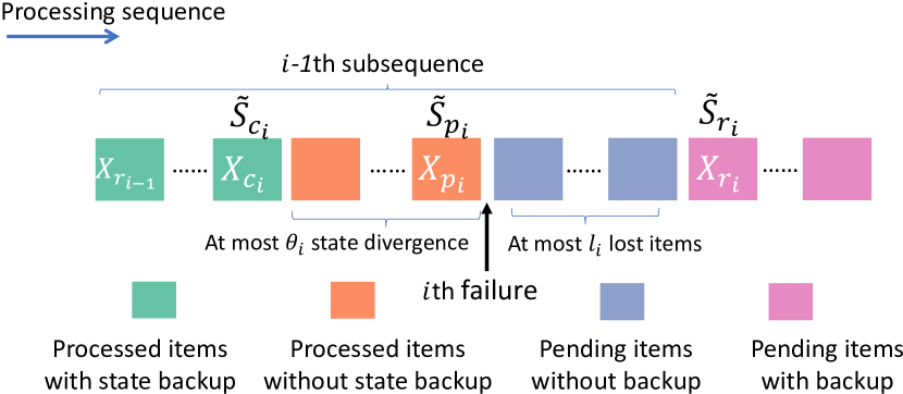
Proof of Theorem 1.
We prove Theorem 1 based on above lemmas. We define the following notation (see Figure 13 for illustration). Suppose that the -th failure happens right after an item, denoted by is processed. To recover from the failure, AF-Stream loads the most recent checkpoint state (i.e., the model parameters), denoted by , which corresponds to the state vector of SGD after the item has been processed. It also resumes SGD from some recovered item, denoted by , where . We can equivalently view that the model updates from to are all discarded, and hence for . Without loss of generality, we set .
Upon the recovery of the -th failure, let denote the divergence between the recovered state and the actual state before the failure, be the number of lost items that are not yet processed and have no backup, and be the state divergence incurred by each lost item. Note that and are dynamic thresholds with respect to and , respectively, and they both decrease as increases to bound the overall errors (see details below). Also, is expected to be bounded in any well-defined machine learning model; otherwise the model becomes unstable. Thus, the total state divergence is .
Our proof has three parts: (i) split all items into subsequences due to failures, (ii) apply Lemma 4 to bound the error of each subsequence, and (iii) sum up the errors of all subsequences.
(i) We first split the sequence into subsequences:
(ii) We next bound the difference of each subsequence. However, for each , we cannot apply Lemma 4 directly since the condition does not hold for . To compensate, we construct another subsequence for , where and for . Then Lemma 4 works for the concatenation of the two subsequences and .
(iii) Finally, we sum up the differences of all subsequences.
To prove Theorem 1, we need to bound three terms: , , and . The first two terms can be bounded by halving and after each failure recovery to make the sum of a geometric series bounded (§3.5.2 and §3.5.3). Specifically, if the initial values are set to be and , we have . For the term , since each must be smaller than , we have .
We can now bound the sum of the differences of all subsequences as follows:
By dividing both sides by , the error is negligible when approaches infinity, i.e.,
Remarks.
In the proof of Theorem 1, the parameters and are used to bound the term . Note that the effect of has already been included in state divergence (i.e., the distance is the accumulated result of unacknowledged processed items), so our proof does not include .
Convergence rate.
AF-Stream has a (slightly) slower convergence rate than the standard SGD. Specifically, the regret difference to the optimum is , while the regret difference is in the failure-free case based on Lemma 4. This implies that AF-Stream requires more steps to achieve the same error level. Nevertheless, our experiments show that the number of extra steps is limited.
Extensions for other optimization methods.
While our analysis focuses on SGD, another well-known class of methods for learning parameters in machine learning is Markov Chain Monte Carlo (MCMC). In particular, Gibbs sampling is one well-known MCMC method, and its efficiency for the Latent Dirichlet Allocation (LDA) model has been well-justified [18, 78, 66, 4]. Even though we cannot apply our analysis of SGD directly to MCMC methods, we briefly discuss how their models converge under AF-Stream. In particular, the divergence from the states to a stationary distribution only depends on how many times the model is updated, i.e., the number of successfully processed items [18]. Since the errors in AF-Stream are equivalent to dropping a bounded number of model updates, AF-Stream still ensures model convergence with sufficient input items.
Appendix C Interfaces and Built-in Primitive Operators in AF-Stream
| Entities | Functions | Descriptions |
| Worker | void AddUpstreamWorker(string& upName) | Adds an upstream worker |
| void AddDownstreamWorker(string& downName) | Adds a downstream worker | |
| void AddUpstreamThread(Thread& thread) | Plugs in the upstream thread | |
| void AddDownstreamThread(Thread& thread) | Plugs in the downstream thread | |
| void AddComputeThread(Thread& thread) | Plugs in a compute thread | |
| void PinCPU(Thread& thread, int core) | Pins a thread to a CPU core | |
| void SetWindow(int type, int length) | Sets the type and length of a window (the window type can be the hopping window, the sliding window, or the decaying window) | |
| void Start() | Starts the execution of the worker | |
| Compute | void ConnectFromUpstreamThread() | Associates the compute thread with the upstream thread |
| thread | void ConnectToDownstreamThread() | Associates the compute thread with the downstream thread |
| void ConnectToComputeThread(Thread& dstThread) | Connects the compute thread to another compute thread | |
| void SendToUp(string& upName, Item& feedback) | Sends a feedback item to an upstream worker | |
| void SendToDown(string& downName, Item& data) | Sends a data item to a downstream worker |
| Entities | Functions | Descriptions |
| Upstream thread | Item ReceiveDataItem() | Receives an input item from data sources or upstream workers |
| int GetDestComputeThread(Item& item) | Returns the compute thread which an item is dispatched | |
| void SendFeedbackItem(Item& feedback) | Sends a feedback item to an upstream worker | |
| Downstream thread | void SendDataItem(Item& feedback) | Sends output items |
| Item ReceiveFeedbackItem() | Receives a feedback item from downstream workers | |
| Compute thread | bool ProcessData(Item& data) | Processes a data item |
| bool ProcessFeedback(Item& feedback) | Processes a feedback item | |
| bool ProcessPunctuation(Item& punc) | Processes a punctuation item | |
| Fault-tolerant operator | double StateDivergence() | Gets the divergence of the up-to-date state and the backup state |
| State BackupState() | Returns the state to be saved by AF-Stream | |
| void RecoverState(State& state) | Obtains the most recent backup state from AF-Stream |
| Operator | StateDivergence | BackupState | RecoverState |
| Numeric variables | Difference of two values | Returns the variable value | Assigns the variable value |
| Vector and matrix | Manhattan distance; Euclidean distance; or maximum difference of values of an index | Returns a list of (index, value) pairs and the length of the list | Fills in restored (index, value) pairs |
| Hash table | Manhattan distance, Euclidean distance, maximum difference of values of a key, difference of the numbers of keys | Returns a list of (key, value) pairs and the length of the list | Inserts the restored (key, value) pairs |
| Set | Difference of the numbers of keys | Returns a list of set members and the length of the list | Inserts the restored set members |