Constraining the three-dimensional orbits of galaxies under ram pressure stripping with convolutional neural networks

Abstract

Ram pressure stripping (RPS) of gas from disk galaxies has long been considered to play vital roles in galaxy evolution within groups and clusters. For a given density of intracluster medium (ICM) and a given velocity of a disk galaxy, RPS can be controlled by two angles ($\theta$ and $\phi$) that define the angular relationship between the direction vector of the galaxy’s three-dimensional (3D) motion within its host cluster and the galaxy’s spin vector. We here propose a new method in which convolutional neutral networks (CNNs) are used to constrain $\theta$ and $\phi$ of disk galaxies under RPS. We first train a CNN by using $\sim 10^{5}$ synthesized images of gaseous distributions of the galaxies from numerous RPS models with different $\theta$ and $\phi$. We then apply the trained CNN to a new test RPS model to predict $\theta$ and $\phi$. The similarity between the correct and predicted $\theta$ and $\phi$ is measured by cosine similarity ($\cos\Theta$) with $\cos\Theta=1$ being perfectly accurate prediction. We show that the average $\cos\Theta$ among test models is $\approx 0.95$ ($\approx 18^{\circ}$ deviation), which means that $\theta$ and $\phi$ can be constrained by applying the CNN to the gaseous distributions. This result suggests that if the ICM is in hydrostatic equilibrium (thus not moving), the 3D orbit of a disk galaxy within its host cluster can be constrained by the spatial distribution of the gas being stripped by RPS. We discuss how this new method can be applied to H i studies of galaxies by ongoing and future large H i surveys such as the WALLABY and the SKA projects.

1 Introduction

Since the crucial influences of ram pressure stripping (RPS) on galaxy evolution was pointed out by idealized models of RPS by Gunn & Gott (1975), the roles of RPS in galaxy evolution within groups and clusters of galaxies have been investigated both observationally and theoretically by many astronomers (e.g., Abadi et al. 1999; Vollmer et al. 2001; Roediger et al. 2005; Kawata & Mulchaey 2008; McCarthy et al. 2008; Kronberger et al. 2008; Tonnesen & Bryan; Bekki 2014, B14). For example, rapid gas removal of cold interstellar medium (ISM) by RPS is responsible for the transformation from gas-rich spiral galaxies into gas-poor S0s (e.g., Quills et al. 2000; Boselli et al. 2006). Galaxy-wide gas distributions and star formation processes can be severely influenced by RPS in disk galaxies within massive groups and clusters (e.g., Bekki & Couch 2003; Crowl et al. 2005; Kenney et al. 2015). The molecular contents and dust of disk galaxies can be also influenced by RPS (e.g., Wong et al. 2014; Cortese et al. 2016; Jachym et al. 2017; Henderson & Bekki 2016).

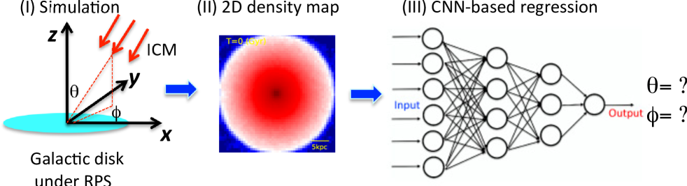
Figure 1: Illustration of the new method to infer the direction of 3D motion of a disk galaxy under strong RPS. The 3D motion with respect to ICM is specified by $\theta$ and $\phi$ (shown in the left part of this figure). The new method consists of the following two components: (i) training a CNN based on a larger number of 2D gas density maps of disk galaxies constructed from numerical simulations and (ii) applying the trained CNN to 2D gas density maps of new models (that are not used in the training of the CNN) to predict $\theta$ and $\phi$.

The strength of RPS for a disk galaxy moving in a cluster of galaxies can be determined largely by the following four parameters (Gunn & Gott 1975; Abadi et al. 1999; Bekki 2009): the ICM density ($\rho_{\rm icm}$), the relative velocity between the galaxy and the ICM ($V_{0}$), and the two angles ($\theta$ and $\phi$) that specify the difference between the direction vector of the relative velocity and the spin vector of the galaxy. Since $\rho_{\rm icm}$ can be inferred from a combination of theoretical models for ICM in hydrostatic equilibrium and X-ray observations of gas (e.g., Matsumoto et al. 2000), $V_{0}$, $\theta$, and $\phi$ are parameters for RPS that appear to be difficult to be constrained by observations. Theoretical models of galaxy formation in clusters provided a prediction on the typical orbital eccentricity ($e_{\rm o}$) for cluster member galaxies (e.g., Ghigna et al. 1998), and the total mass of a cluster ($M_{\rm cl}$) can be informed from other observations (e.g., line-of-sight velocities, $v_{\rm los}$, of cluster member galaxies and X-ray emission from hot ICM). Accordingly, $V_{0}$ of a galaxy in a cluster can be inferred from its (projected) position within the cluster with the observationally estimated $M_{\rm cl}$ (by using the observed $v_{\rm los}$ of the galaxy) and the typical $e_{\rm o}$, though such inference can not be so accurate. Thus $\theta$ and $\phi$ are the key parameters of RPS that appear to be very hard to be constrained by observations and theoretical models.

If $\theta$ and $\phi$ are derived by a comparison between observations and simulations, then such derivation can have the following important implications. Since the inclination angles ($\theta_{\rm v}$ and $\phi_{\rm v}$) of a disk galaxy on the sky can be easily estimated by observations, the derived $\theta$ and $\phi$ can be converted into the direction vector (u) of the galaxy’s motion using $\theta_{\rm v}$ and $\phi_{\rm v}$. Based on u, the 3D orbit of the galaxy within the cluster can be discussed, if the total velocity ($v_{\rm t}$) of the galaxy can be inferred from other observations and theoretical models: it should be noted, however, such inference of $v_{\rm t}$ should be quite difficult. These points are discussed in §4 of this paper. The derived $\theta$ and $\phi$ could be also correlated with other physical properties of galaxies under RPS, such as the spatial distributions of star-forming regions, because RPS can suppress ISM to enhance star formation and $\theta$ and $\phi$ can be key parameters for this process (B14). For example, if $\theta\approx 0^{\circ}$ in a disk galaxy, then the disk’s outer edge (confronting with the ICM compression) shows an enhanced star formation. These correlations accordingly can possibly improve our understanding of how RPS can influence galaxy-wide star formation in clusters. Furthermore, the 3D orbits of galaxies have been discussed by previous cosmological simulations of clusters of galaxies (e.g., Ghigna et al. 1998). Thus, inference of $\theta$ and $\phi$ can have some benefits in understanding galaxy evolution in clusters.

The purpose of this paper is to constrain $\theta$ and $\phi$ of disk galaxies under RPS using convolutional neutral networks (CNNs). CNNs have been fundamental elements in recent classification technique using deep learning, and they have been recently applied to morphological classification of galaxies. For example, Dieleman et al. (2015) demonstrated how artificial intelligence can automate the classification of galaxy morphologies by training a CNN on the crowdsourced classifications of the Galaxy Zoo project (see also more recent work by Dominguez Sanchez et al. 2018). In the present work, we explore the prediction of $\theta$ and $\phi$ using CNN techniques on 2D images of the simulated gas content. It is well known that the detailed distributions of galactic cold gas being stripped by RPS depend on $\theta$ and $\phi$ (e.g., Abadi et al. 1999; B14). Accordingly, the gaseous distributions can have information on $\theta$ and $\phi$. We use a larger number ($>10^{4}$) of the (projected) 2D gaseous distributions of disk galaxies under RPS as input dataset to train a CNN in the present study. Once the trained CNN is found to predict accurately $\theta$ and $\phi$, then we use it for testing new dataset.

The plan of the paper is as follows. We describe the models of RPS in gas-rich disk galaxies within clusters and the new way to infer $\theta$ and $\phi$ of the galaxies using CNNs in §2. We present the results of numerical simulations of disk galaxies under strong RPS to discuss the accuracy of predictions on $\theta$ and $\phi$ of the galaxies for various test models in §3. Based on these results, we provide several implications of the present results and discuss how we can prove the accuracy of the predictions in our future works in §4. We summarize our conclusions in §5.

2 The model

2.1 The outline

Fig. 1 illustrates the three basic components of the present study. First, we run numerous RPS models with different $\theta$ and $\phi$ for different initial models of RPS (e.g., ICM density determined by the 3D positions of disk galaxies). We then investigate the 2D density maps of cold gas using the results of hydrodynamical simulations. These 2D density maps (referred to as “images”) are input into a CNN so that the CNN can be well trained for accurate predictions of $\theta$ and $\phi$. Finally, the trained CNN is used to predict the 3D motion of a disk galaxy under RPS with respect to ICM (defined by $\theta$ and $\phi$) for each of test models that are not used in the training phase of the CNN. This new CNN-based method to predict $\theta$ and $\phi$ from simulation dataset is essentially similar to those adopted in our recent studies.

Since we adopt the same RPS model used in our previous paper (B14), we briefly describe the model in the present paper. In B14, the orbit of a disk galaxy within its host cluster galaxy is first calculated for a given set of initial conditions (e.g., the 3D position of the galaxy with respect to the cluster center) using the adopted gravitational potential of the cluster. Then the strength of RPS is self-consistently estimated at each time step in each model so that the details of RPS of gas can be investigated. In the present study, we do not discuss much about the orbits of disk galaxies in its host cluster.

2.2 Disk galaxy

A disk galaxy is assumed to move in a cluster of galaxies and the ram pressure force of the ICM on the disk galaxy is calculated according to the position and velocity of the galaxy with respect to the cluster center. We use our original chemodynamical simulation code that can be run on GPU machines (Bekki 2013, B13) in order to investigate the details of the spatial distribution of gas in disk galaxies under RPS at different times steps. A disk galaxy is composed of dark matter halo, stellar disk, stellar bulge, and gaseous disk, and we mainly investigate luminous MW-like disk models in which the mass ratio of the dark matter halo ($M_{\rm h}$) to the disk ($M_{\rm s}+M_{\rm g}$) in a disk galaxy is fixed at 16.7 and $M_{\rm h}=10^{12}{\rm M}_{\odot}$. We adopt the ‘NFW’ profile for the dark matter halo (Navarro, Frenk & White 1996) suggested from CDM simulations with the $c$-parameter of 10 and the virial radius of 245 kpc.

The mass and size of the galactic bulge in a disk galaxy are free parameters denoted as $M_{\rm b}$ and $R_{\rm b}$, respectively. The radial ($R$) and vertical ($Z$) density profiles of the adopted exponential stellar disk are assumed to be proportional to $\exp(-R/R_{0})$ with scale length $R_{0}=0.2R_{\rm s}$ and to ${\rm sech}^{2}(Z/Z_{0})$ with scale length $Z_{0}=0.04R_{\rm s}$, respectively. The gas disk with a size $R_{\rm g}=R_{\rm s}$ has the radial and vertical scale lengths of $0.2R_{\rm g}$ and $0.02R_{\rm g}$, respectively. The disk of the present MW model has $R_{\rm s}=17.5$ kpc and In addition to the rotational velocity caused by the gravitational field of disk, bulge, and dark halo components, the initial radial and azimuthal velocity dispersions are assigned to the disc component according to the epicyclic theory with Toomre’s parameter $Q$ = 1.5. The gas mass fraction ($f_{\rm g}=M_{\rm g}/M_{\rm s}$) is also a free parameter.

We mainly investigate the “Milky-Way (MW)” model with $M_{\rm b}=10^{10}{\rm M}_{\odot}$, $R_{\rm b}=3.5$ kpc, and $f_{\rm g}=0.1$ in the present study. This MW model is used for RPS models to train a CNN. We also investigate “Sa” models with a larger bulge-to-disk-ratio of 0.5 (i.e., $M_{\rm b}=3\times 10^{10}{\rm M}_{\odot}$) and $f_{\rm g}=0.1$ and “Sd” bulge-less disk models with $M_{\rm b}=0$ and $f_{\rm g}=0.2$. These two models are not used in the training of a CNN and rather it is used in RPS simulations as test models for the trained CNN in the present study. It would not be enough for the present study to use only three different Hubble types to train/test a CNN. However, since this study is the first step toward a very accurate prediction of 3D motion of a disk galaxy under RPS, we consider that investigation of RPS models based on the three different initial disk models can be more than enough.

Star formation, chemical evolution, dust evolution, metallicity-dependent radiative cooling, feedback effects of supernovae, formation of molecular gas are all included in the present study, and the details of these modeling are given in B13 and Bekki (2015). The Kennicutt-Schmidt law for galaxy-wide star formation (e.g., Kennicutt 1998) is adopted the threshold gas density for star formation being 1 atom cm^-3. The initial central metallicity of gas in a disk ([Fe/H]₀) is set to be 0.34 and the radial metallicity gradient is $-0.04$ dex kpc^-1. The formation of molecular hydrogen from neutral one on dust grains is properly modeled using the dust abundance of gas and the interstellar radiation field around the gas. Chemical yields for SNIa and SNII and those for AGB stars are adopted from Tsujimoto et al. (1995; T95) and van den Hoek and Groenewegen (1997; VG97), respectively. The dust growth and destruction timescales ($\tau_{\rm acc}$ and $\tau_{\rm dest}$, respectively) are set to be 0.25 Gyr and 0.5 Gyr, respectively. The canonical Salpeter initial mass function of stars (IMF) with the exponent of IMF being $-2.35$ is adopted.

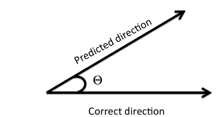
Figure 2: Illustration of a way to quantify the cosine distance (similarity) between correct and predicted direction vectors of galaxy motion for a model. The correct and predicted vectors are specified by two angles, $\theta_{\rm c}$ and $\phi_{\rm c}$ for the correct vector, and $\theta_{\rm p}$ and $\phi_{\rm p}$ for the predicted vector. The angle between the correct and predicted vectors is demoted as $\Theta$, and $\cos\Theta$ is considered to measure the level of similarity between the two vectors.

2.3 Time-varying ram pressure force

We consider that a disk galaxy within its host cluster of galaxies is embedded in hot ICM with temperature $T_{\rm ICM}$, density ${\rho}_{\rm ICM}$, and velocity $V_{\rm r}$. Here the relative velocity of ICM with respect to the velocity of the disk galaxy is denoted as $V_{\rm r}$. The ICM surrounding the disk galaxy is represented by SPH particles in a cube with the size ($R_{\rm box}$) of $3R_{\rm g}$ (where $R_{\rm g}$ is the initial gas disk size corresponding to the stellar disk size in the present work). This value of $3R_{\rm g}$ is demonstrated to be large enough to model RPS in disk galaxies (B14). This “bound box model” is adopted in previous works (e.g., Abadi et al. 1999; B14) so that a huge particle numbers to represent the entire ICM in clusters of galaxies can be avoided. The galaxy is initially located at the exact center of the cube and the direction of the orbit (within a cluster) is the $x$-axis in the Cartesian coordinate of the cube.

Since we follow the orbit of the galaxy under the adopted cluster potential (constructed from the NFW profile), we can investigate both ${\rho}_{\rm ICM}$ and velocity $V_{\rm r}$ self-consistently at each time step. Accordingly, we consider that the strength of ram pressure force on the disk should be time-dependent and described as follows:

$$P_{\rm ram}(t)=\rho_{\rm ICM}(t)V_{\rm r}^{2}(t),$$ (1)

where ${\rho}_{\rm ICM}(t)$ and $V_{\rm r}$(t) are determined by 3D positions and velocities of a galaxy at each time step in a simulation, as described in B14. The total mass of ICM within the cubic box is therefore time-dependent as follows:

$$M_{\rm ICM}(t)=\rho_{\rm ICM}(t)R_{\rm box}^{3}.$$ (2)

Accordingly, $M_{\rm ICM}(t)$ is different from its initial value ($M_{\rm ICM,0}$) at the start of a simulation. Each ICM gas particle therefore needs its mass ($m_{\rm ICM}$) to change with time according to the change of $M_{\rm ICM}$. For example, when a galaxy is approaching to the core of its host cluster, then $m_{\rm ICM}$ can increase with time.

The total ICM mass with a cubic box at the starting time of a simulation is not significantly larger than the total gas mass of a disk galaxy. For example, $M_{\rm ICM}$ is $1.1\times 10^{10}{\rm M}_{\odot}$ in the fiducial RPS model (described in Table 1), which means that $m_{\rm ICM}$ is about 60% of the adopted mass resolution ($m_{\rm g}$) for the gas disk if $40^{3}$ meshes in the cubic box are adopted: if $60^{3}$ meshes are adopted (B14), $m_{\rm ICM}$ can be significantly smaller than $m_{\rm g}$. Accordingly, the present simulations can avoid the overestimation of RPS effects caused by $m_{\rm ICM}$ much larger than $m_{\rm g}$. The ICM mass can change with time in the simulations, however, $m_{\rm ICM}$ can not be too much larger than $m_{\rm g}$ in the present study. We mainly investigate the “Coma” cluster model with $M_{\rm h}=10^{15}{\rm M}_{\odot}$ and $T_{\rm ICM}=1.2\times 10^{8}$ K, because RPS is quite efficient in most of galaxies close to the cluster core (B14).

In the following simulations, the spin axis of a disk galaxy under RPS is specified by two angle $\theta$ and $\phi$ (in units of degrees): $\theta$ is the angle between the $z$-axis and the vector of the spin of a disk and $\phi$ is the azimuthal angle measured from $x$-axis to the projection of the spin vector of a disk on to $xy$ plane. The direction of ram pressure force with respect to gaseous motion in a local region of a galaxy depends strongly on these two angles $\theta$ and $\phi$. This is a main reason why $\theta$ and $\phi$ can be inferred from the spatial distribution of gas influenced by RPS. The initial position of the disk galaxy is set to be ($x$, $y$, $z$)=($R_{\rm i}$, 0, 0), where $R_{\rm i}$ is the initial distance of the galaxy from the center of its host cluster as follows:

$$R_{\rm i}=f_{\rm p}R_{\rm vir}$$ (3)

where $f_{\rm p}$ is a free parameter that controls the initial position and ranges from 0.1 and 0.5. The initial velocity of the galaxy is set to be ($V_{\rm x}$, $V_{\rm y}$, $V_{\rm z}$)=(0, $V_{\rm i}$, 0), where $V_{\rm i}$ is as follows:

$$V_{\rm i}=f_{\rm v}v_{\rm c}$$ (4)

where $v_{\rm c}$ is the circular velocity of the galaxy at its initial position within the host cluster. This parameter $f_{\rm v}$ is set to range from 0.5 to 0.7. In these modeling of initial positions and velocities of a galaxy in a cluster, we consider that the gravitational potential of the cluster is spherical symmetric just for simplicity. The present simulations are different from B14 in the sense that galaxies are initially within the virial radius of their host cluster. This is mainly because B14 already found that RPS can not strip the gas disks significantly until they become close to the inner regions of their cluster (see Fig. 2 in B14). Since the main purpose of this paper is to investigate the 2D density maps of galaxies under strong RPS, such modeling of galaxies (i.e., starting from strong RPS phases) would not be a problem.

Table 1: Description of the basic parameter values for the fiducial RPS model (T0) in a massive cluster of galaxies.

Physical properties	Parameter values
Total cluster mass	$M_{\rm dm}=1.0\times 10^{15}{\rm M}_{\odot}$
Cluster virial radius	$R_{\rm vir}=2.69$ Mpc
$c$ parameter of cluster halo	$c=3.6$
ICM mass	$M_{\rm icm}=1.5\times 10^{14}{\rm M}_{\odot}$
ICM temperature	$T_{\rm icm}=1.2\times 10^{8}$ K
Total halo mass (galaxy)	$M_{\rm dm}=1.0\times 10^{12}{\rm M}_{\odot}$
DM structure (galaxy)	NFW profile
Galaxy virial radius (galaxy)	$R_{\rm vir}=245$ kpc
$c$ parameter of galaxy halo	$c=10$
Stellar disk mass	$M_{\rm s}=6.0\times 10^{10}{\rm M}_{\odot}$
Stellar disk size	$R_{\rm s}=17.5$ kpc
Gas disk size	$R_{\rm g}=17.5$ kpc
Disk scale length	$R_{0}=3.5$ kpc
Gas fraction in a disk	$f_{\rm g}=0.1$
Bulge mass	$M_{\rm b}=10^{10}{\rm M}_{\odot}$
Bulge size	$R_{\rm b}=3.5$ kpc
Mass resolution	$3.0\times 10^{5}{\rm M}_{\odot}$
Size resolution	252 pc
Initial ICM mass ($M_{\rm ICM,0}$)	$1.1\times 10^{10}{\rm M}_{\odot}$
Time-dependent $M_{\rm ICM}$	Included
Star formation law	The KS law with $\rho_{\rm th}=1$ ${\rm cm}^{-3}$
Initial central metallicity	${\rm[Fe/H]_{0}}=0.34$
Initial metallicity gradient	$\alpha_{\rm d}=-0.04$ dex kpc-1
Chemical yield	T95 for SN, VG97 for AGB
Dust yield	B13
Dust formation model	$\tau_{\rm acc}=0.25$ Gyr, $\tau_{\rm dest}=0.5$ Gyr
Initial dust/metal ratio	0.4
${\rm H_{2}}$ formation	Dependent on dust abundance (B13)
Feedback	SNIa and SNII (no AGN)
IMF	The canonical IMF

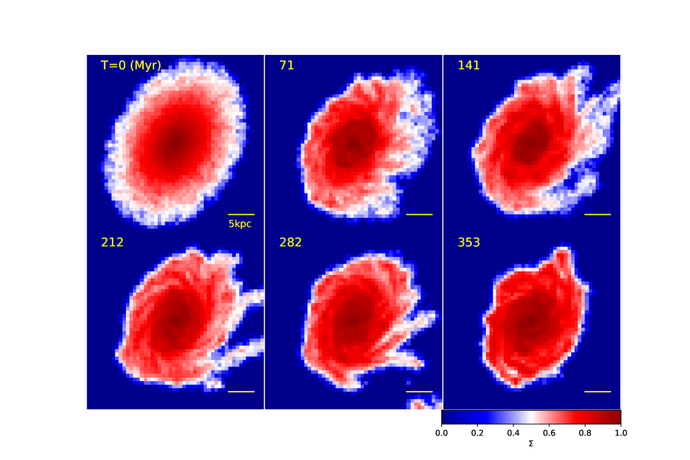
Figure 3: Time evolution of the surface mass density ($\Sigma$ in logarithmic scale) of gas in a disk galaxy under strong RPS projected onto the $x$-$y$ plane for the fiducial model with $\theta=30$ degrees, $\phi=45$ degrees, $f_{\rm p}=0.3$, and $f_{\rm v}=0.5$. Time ($T$) that has elapsed since the start of this simulation is shown in the upper left corner of each frame. The scale bar of 5 kpc is shown in the lower right at each panel. The mass density at each frame is normalized using all pixel values in each image (produced at each time step) so that the minimum and maximum density can be 0 and 1, respectively. $50\times 50$ meshes are used to produce these images in this model.

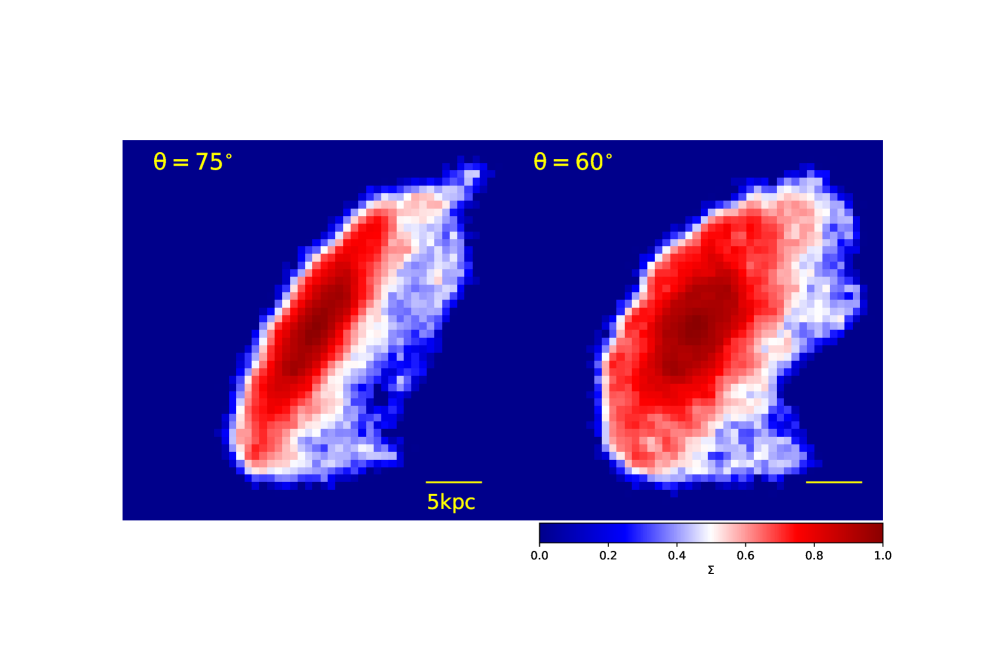
Figure 4: The same as Fig. 3 but for the models with $\theta=75^{\circ}$ (left) and $\theta=60^{\circ}$ (right) at $T=71$ Myr. For these models, $\phi$ is fixed at $30^{\circ}$. These can be compared with the 2D density map at $T=71$ Myr in Fig. 3.

2.4 2D density and velocity map

In order to train the CNN, we need to produce a larger number of 2D mass-density and (line-of-sight) velocity maps (often referred to as “images” ) for simulated galaxies using the projected positions and the line-of-sight velocities ($V_{\rm los}$) of gaseous particles of the galaxies. We use only the 2D gas density maps to train a CNN in the present paper, however, we also explain the way to produce normalized velocity map too, because they are shown to describe the effects of RPS on stellar kinematics of disk galaxies. The 2D velocity (kinematic) maps of cold gas in disk galaxies will be used to improve the accuracy of CNN-based predictions in our future papers.

We here try to derive the 2D density maps of simulated galaxies for $R\leq R_{\rm g}$. We first divide the gas disk ($R\leq R_{\rm g}$) of a galaxy into $50\times 50$ small areas (meshes) and estimate the mean gas density at each mesh point. The projected mass density of gas in a simulated galaxy can be estimated as follows:

$$\Sigma_{i,j,0}=\frac{1}{{\Delta R_{i,j}}^{2}}\sum_{k=1}^{N_{\it i,j}}m_{k},$$ (5)

where $\Delta R_{i,j}$, $N_{i,j}$, and $m_{k}$ are the mesh size at the mesh point ($i$, $j$), the total number of gas particles in the mesh, and the mass of a gas particle, respectively. In training a CNN, we use the logarithm of $\Sigma_{i,j,0}$ to base 10 as follows:

$$\Sigma_{i,j}=\log_{10}\Sigma_{i,j,0}.$$ (6)

The mesh size is $0.04R_{\rm g}$ which corresponds roughly to 0.7 kpc for a Milky Way-type disk galaxy. We also smooth out the density (velocity) field using a Gaussian kernel with the smoothing length ($h_{\rm sm}$) of $0.05R_{\rm s}$ (0.86 kpc). This smoothing is to mimic an observational resolution (e.g., beam size of a radio telescope) in a large survey of galaxies such as the WALLABY project. We discuss how the present results can depend on $h_{\rm sm}$ in §4 later. We need to normalize the 2D data in order to feed the data into CNNs, and the normalized 2D gas density map can be derived as follows:

$$\Sigma_{i,j}^{\prime}=\frac{\Sigma_{i,j}-\Sigma_{\rm min}}{\Sigma_{\rm max}-\Sigma_{\rm min}},$$ (7)

where $\Sigma_{\rm min}$ and $\Sigma_{\rm max}$ are the minimum and maximum values of $\Sigma$ among the $50\times 50$ meshes in a model for a given projection. This normalization procedure is taken for each image at each time step. This procedure of normalization ensures that the 2D density ranges from 0 to 1. Therefore, the normalization factor is different in different models with different projections.

Figure 5: Normalized distribution of $\cos\Theta$ for the fiducial test model T0. The vertical dotted line represents the mean $\cos\Theta$ in this model. Cosine similarity ($\cos\Theta$) is derived for each of 10,000 2D gas density maps (images) and the total number of images in each $\Theta$ bin ($N_{\rm t}$) is counted. This $N_{\rm t}$ distribution is normalized by the maximum number of $N_{\rm t}$ in this figure for clarity.

2.5 CNN architecture

The adopted CNN architecture consists of 2 convolutional layers (“Conv2D”), and 1 max pooling layers (“Max Pool”), two dropout layers (“Dropout”), 1 flatten layer (“Flatten”), 1 fully connected layers (“FC1”), and output layer (“Output”). Conv2D is a neutral network layer (NNL) that performs two-dimensional (2D) layer convolution whereas Max Pooling is a NNL that can reduce the size of the state of the network through down-sampling based on the highest pixel value in each region. Flatten is a NNL that is designed to reshape vector shapes inside a network into a 1D vector, and Dropout is a NNL can reduce the probability of over-fitting in a network by randomly nulling a certain percentage of neurons in a previous layer. FC1 is a NNL in which all neurons are connected between two layers.

The filter size is $3\times 3$ for Conv2D and $2\times 2$ for Max Pool. The drop out rate is set to be 25% and 50% for the first and second Dropout layers, respectively, so that over-fitting can be avoided during CNN training. ReLu activation function is adopted for Conv2D and FC1 whereas linear one is adopted for Output. The “ADADELTA” (Adaptive Learning Rate Method; Zeiler 2012) is adopted for gradient descent in the training phase of a CNN.

These CNN settings of Conv2D, Max Pool, FC1, Output layers are almost exactly the same as those adopted in Bekki et al. (2018): the linear activation function instead of the softmax is adopted in the present study. In order to develop the above CNN through supervised learning based on a lager number of images from simulations, we use the publicly available Keras (Chollet 2015) which is a collection of neutral network libraries for deep learning. The details of the CNN architecture and the basic method to determine $\theta$ and $\phi$ by applying the Keras code to the 2D density maps of gas from simulated and observed galaxies are given in Appendix A.

2.6 Training CNNs

We use 60,000 synthesized images of 2D gaseous distributions constructed from 600 RPS models with the MW-type initial disk and different sets of RPS parameters ($\theta$, $\phi$, $f_{\rm p}$ and $f_{\rm v}$) for 100 viewing angles (per RPS model). The two viewing angles, $\theta_{\rm v}$ and $\phi_{\rm v}$, are evenly distributed across the $theta$- and $\phi$-directions (i.e., not selected using a random number generator). For this training set of data, the results at $T=71$ Myr are used to produce the images: multiple images from a single galaxy is used for training the CNN.

These RPS parameters are chosen randomly using a random number generator. These RPS models used for this training phase are referred to as “TR1”, and the model parameters are briefly summarized in Table 2. We also trained a CNN using 60,000 images of gaseous distributions constructed from RPS models (“TR2”) for which the RPS parameters are chosen by using a random number generator with the seed number being different from the one used in TR1. Since we found that the predictions of $\theta$ and $\phi$ of test models based on the CNN trained by TR2 are essentially similar to those by TR1, we show only the predictions from the CNN trained by TR1 in the present paper.

The CNN is trained for 100, 300, and 1000 epochs ($N_{\rm epoch}$) so that the “accuracy rate” ($R_{\rm a}$), which is defined as the mean of $\cos\Theta$ for all models here, can be very high ($0.998$, corresponding to deviation of $\Theta\approx 3.6^{\circ}$). We confirm that $R_{\rm a}$ is almost identical between $N_{\rm epoch}=300$ and 1000 (i.e., no need to train CNNs for more than $N_{\rm epoch}=300$). The NVIDIA GPU GTX1080 on the “Pleiades” GPU cluster at the University of Western Australia is used to train a CNN in the present study. It takes 6.5 CPU/GPU hours to train a CNN with the total input images ($N_{\rm i}$) of 60,000 for $N_{\rm epoch}=300$. The number of images fed into a CNN in the training phase of the CNN is limited by the available CPU memory of the Pleiades GPU cluster. Although the required CPU/GPU time is not a limitation in the present study, $N_{\rm i}$ that can be fed into the GPU cluster is a strong limitation in the present study.

2.7 Cosine similarity

The two angles $\theta$ and $\phi$ predicted by the trained CNN for each model (defined as $\theta_{\rm p}$ and $\phi_{\rm p}$, respectively) needs to be compared with the correct (i.e., initially set) $\theta$ and $\phi$ (defined as $\theta_{\rm c}$ and $\phi_{\rm c}$, respectively) so that the accuracy of the prediction can be measured. In order to quantify the accuracy of the prediction by the trained CNN for each model, we use the cosine similarity method (e.g., Singhal 2001). In this method, we consider the following two vectors: one (u_c) is ($\theta_{\rm c}$, $\phi_{\rm c}$), which describes the “correct direction”, and the other (u_p) is ($\theta_{\rm p}$, $\phi_{\rm p}$), which describes the “predicted direction”. It should be noted here that the two vectors are defined in the $\theta$-$\phi$ plane. We first normalize these two vectors so that the values of $\theta$ and $\phi$ can range from 0 to 1. Then we calculate the inner product in each model using the normalized vectors: the cosine similarity, however, is not different between models with and without this normalization. Accordingly, the cosine similarity (or distance) between the two normalized vectors (defined as $\cos\Theta$) for each image is as follows:

$$\cos\Theta=\theta_{\rm c}\theta_{\rm p}+\phi_{\rm c}\phi_{\rm p}.$$ (8)

Since each test model produces numerous images ($\geq 10^{4}$), we make an average of $\cos\Theta$ in each test model as follows:

$$\cos\Theta_{\rm m}=\frac{1}{N}\sum_{k=1}^{N}\cos\Theta_{k},$$ (9)

where $N$ is the total number of images for the model. Fig. 2 illustrates the adopted cosine similarity method very briefly. It should be stressed here that an apparently large $\cos\Theta$ value (e.g., $>0.8$) does not mean a high level of consistency between predicted and correct angles.

2.8 Accuracy test for representative models

Using the trained CNN, we investigate whether $\cos\Theta$ in new test models that are not used in training the CNN can be quite high ($>0.95$). Although we investigated numerous models with different model parameters, we mainly describe the results of ten representative models (T0 - T9) in the present study. The fiducial model with a fixed $\theta$ and $\phi$ is referred to as T0, and it is most extensively discussed in the present paper. Table 1 briefly summarizes the model parameter for T0. For each of these ten models, $\theta$ and $\phi$ are inferred for 10,000 images using the trained CNN. The parameter values for these test models and TR1 and the mean $\cos\Theta$ ($\cos\Theta_{\rm m}$) for the test models are summarized in Table 2. Each set of model (e.g., T1 etc) uses 100 different RPS models with different RPS parameters (for 100 viewing angles). Accordingly, the total number of galaxy models used for training and testing phases are 600 and 1000, respectively. The total number of images used for training and testing phases are 60,000 and 100,000, respectively.

The test models T1, T2, and T3 are those in which $f_{\rm p}$ is different (0.1, 0.3, and 0.5 respectively) for a fixed $f_{\rm v}$ (=0.5). Accordingly, the initial strength of RPS is quite different between the three, though cold gas can be significantly influenced by RPS in these. T4 and T5 are based on RPS models in which $f_{\rm v}$ and $f_{\rm p}$ are changed. The adopted range of $\theta$ in T6 is very narrow ($\theta\leq 30^{\circ}$), because we try to investigate how $\cos\Theta$ depends on $\theta$: we show the results of this model, because we found that the trained CNN can less accurately predict $\theta$ and $\phi$ for lower $\theta$. T7 is different from other models in that the 2D density map at $T=0.14$ Gyr (i.e., different RPS phase) is used for testing in this model. Galaxy types in T8 and T9 are different from other models with the MW-type disk. It is our strategy to use the CNN trained by RPS models with only one galaxy type for testing new RPS models in the present study. If $\cos\Theta$ can be quite high for the testing models with initial disk models that are different from those used in the training phase, such a result can be considered to be promising. This is because it is practically less feasible to generate numerous images of gas distributions from numerous different initial disk models, though such a diversity in disk galaxies is reality.

Table 2: Description of the model parameters for the RPS model used for training CNN (TR1) and 10 representative test models (T0, T1, .. and T9). The model T0 is the fiducial model for which the results are the most extensively discussed. Either the investigated value of a model parameter or the range is shown in each column. Tests by the trained CNN are done at the time $T_{\rm r}$ (6th column), which is time that has elapses since the start of RPS ($T=0$). The mean $\cos\Theta$ estimated from all images of test models and from those produced from test models with $\theta\leq 30^{\circ}$ are shown in the 8th and 9th columns, respectively.

Model ID	$f_{\rm p}$	$f_{\rm v}$	$\theta$ (∘)	$\phi$ (∘)	$T_{\rm r}$ (Myr)	Galaxy type	$\cos\Theta_{\rm m}$ (all)	$\cos\Theta_{\rm m}$ ($\theta\leq 30^{\circ}$)
TR1	$0.1-0.3$	$0.5-0.7$	$0-180$	$0-360$	71	MW	$-$	$-$
T0	$0.1-0.3$	$0.5-0.7$	45	30	71	MW	0.971	$-$
T1	$0.1$	$0.5$	$0-180$	$0-360$	71	MW	0.936	0.797
T2	$0.5$	$0.5$	$0-180$	$0-360$	71	MW	0.949	0.830
T3	$0.7$	$0.5$	$0-180$	$0-360$	71	MW	0.942	0.831
T4	$0.3$	$0.5-0.7$	$0-180$	$0-360$	71	MW	0.941	0.830
T5	$0.1-0.5$	$0.5-0.7$	$0-180$	$0-360$	71	MW	0.924	0.834
T6	$0.3$	$0.5$	$0-30$	$0-360$	71	MW	0.947	0.799
T7	$0.3$	$0.5$	$0-180$	$0-360$	142	MW	0.939	0.810
T8	$0.3$	$0.5$	$0-180$	$0-360$	71	Sd	0.942	0.810
T9	$0.3$	$0.5$	$0-180$	$0-360$	71	Sa	0.940	0.821

3 Results

3.1 Fiducial model

Fig. 3 shows how the 2D density ($\Sigma$) maps of gas in a disk galaxy under RPS in the fiducial model T0 can be influenced by hydrodynamical interaction between cold ISM and hot ICM. The cold ISM is strongly compressed by ICM in the upstream side (corresponding to the left part of the disk) so that a very sharp density cut-off can be clearly seen in the upstream side at $T=71$ Myr (i.e., sudden change in color from blue to red with a small number of white-colored meshes). Stripping of cold ISM can be clearly seen in the downstream side (i.e., right part of the disk), and such stripped gas can form short tails (“tentacles in jerryfish”) at $T=141$ and 212 Myr. The gas disk can become significantly more compact in comparison with the original size at $T=353$ Myr, when a fraction of gas is completely stripped by ram pressure. The highly asymmetric distribution of ISM, sharp edges, in particular, in the upstream side, and characteristic gaseous tails can be used to constrain the direction of galaxy motion (i.e., $\theta$ and $\phi$). It should be noted that this efficient stripping is not due to large mass-ratios of ICM to ISM particles (i.e., not due to numerical artifact). The time evolution of the mass-ratio of ICM to ISM particles ($r_{\rm m}=m_{\rm ICM}/m_{\rm g}$) and some brief discussion on this are given in Appendix C.

The results at $T=71$ Myr in Fig 3 and those in Fig. 4 show that the 2D distributions of gas projected onto the $x$-$y$ plane are appreciably different between models with slightly different $\theta$ ($45^{\circ}$, $60^{\circ}$, and $75^{\circ}$). These results demonstrate that such differences in 2D density map can be used for CNN classification to find the direction of galaxy motion with respect to ICM (i.e., inference of $\theta$ and $\phi$), if the derived characteristic features of gas distributions can be detected in ongoing and future observations. Although the sizes of gas disks in late-type disk galaxies are observed to be significantly larger than their stellar disks, we adopted an assumption of $R_{\rm g}=R_{\rm s}$. Accordingly, the 2D images in Figs. 3 and 4 can represent the relatively high-density (surface density of more than $1{\rm M}_{\odot}$ pc^-2) part of the disk galaxy. We thus suggest that it is feasible for ongoing observations (e.g., WALLABY) to detect such gaseous features. The stripped gas outside the cubic box is not considered in the image production.

Figure 6: The same as Fig. 5 but for nine representative models (T1-T9). All 2D images in each model are used to derive $\cos\Theta$.

The above-mentioned unique features in the 2D density (and kinematic) maps of gas within the disk galaxy under RPS can depend on the direction of the galaxy’s motion specified by $\theta$ and $\phi$. Although human eye could capture such dependence on $\theta$ and $\phi$, it would be almost impossible for human eye to quantify $\theta$ and $\phi$ (e.g., $\theta=30^{\circ}$ or $45^{\circ}$). The directions of gaseous tails emerging from one-side of a disk galaxy, the location of the kink in the zero-velocity curve (discussed in §4), the degree of randomness in the 2D kinematics (§4), and the characteristic 2D kinematics in the gaseous tails (§4) can all be used to distinguish between different $\theta$ and $\phi$. If a CNN is trained by 2D density (and/or kinematic) maps produced from many models with different $\theta$ and $\phi$, then the CNN can learn which features are characteristic for a model with a particular set of $\theta$ and $\phi$. Here we try to train a CNN by using only 2D density maps of gas in disk galaxies under RPS: we will discuss how a combination of 2D density and kinematics maps can improve the accuracy of predictions for $\theta$ and $\phi$ in our forthcoming papers.

In Fig. 5, the CNN trained by 60,000 2D density maps is applied to 10,000 2D density map (images) produced by the fiducial model with $\theta=45^{\circ}$ and $\phi=30^{\circ}$. Fig. 5 clearly shows quite high $\cos\Theta$ ($>0.95$ corresponding to $\Theta<18.2^{\circ}$) for most of images and thus demonstrates that the CNN can accurately predict the direction of galaxy motion in the fiducial model. The cosine similarity is estimated to be higher than 0.98 (corresponding to $\Theta<11.5^{\circ}$) for 54% of the 10,000 images from the fiducial model. The mean $\cos\Theta$ ($\cos\Theta_{\rm m}$) is 0.97, which means that the angle of the correct and predicted vectors is $\approx 13.6$ degrees. Although such a difference in the direction between the two vectors is not extremely small, it clearly demonstrates that a CNN that can accurately predict the direction of galaxy motion with respect to ICM can be developed using 60,000 images. This is quite promising, given that only the MW-type disk galaxy with a fixed bulge fraction is used to train the CNN. It is possible that such a high $\cos\Theta_{\rm m}$ is achieved only in this fiducial model. Therefore, it is important for the present paper to test whether the trained CNN can accurately predict the direction of galaxy motion for other models.

Figure 7: The same as Fig. 6 but for 2D images constructed from models with $\theta\leq 30$ degrees and $0\leq\phi\leq 360$ degrees.

3.2 Accuracy test

Fig. 6 show that all nine representative models with different model parameters show $\cos\Theta$ distributions with high mean $\cos\Theta_{\rm m}$ (ranging from 0.92 to 0.95) that are very similar to those derived in the fiducial model. The mean $\cos\Theta_{\rm m}$ for the nine model is 0.94, which corresponds to 19.9^∘ difference between the correct and predicted vectors for galaxy motion. Although these results confirm that the CNN can accurately predict the direction of galaxy motion for a range of model parameters, the prediction of galaxy motion is not extremely accurate. Accordingly, there is much room for future studies to improve the accuracy of CNN-based prediction for galaxy motion with respect to ICM. Given that only one galaxy type is adopted for training the CNN, increasing the number of galaxy models in the training can possibly improve the accuracy of prediction. This point needs to be confirmed in our future study.

It should be stressed here that the RPS model at a different RPS phase ($T=141$ Myr; the test model T7) shows $\cos\Theta_{\rm m}=0.94$, though the CNN is trained by models at $T=71$ Myr only. It is confirmed that models with $71\leq T\leq 212$ Myr also show high $\cos\Theta_{\rm m}$ ($\approx 0.95$) in the present study. These results imply that we do not need a larger number of models with different RPS phases to train CNNs for predicting the direction of galaxy motion. Furthermore, the models with bulge-to-disk-ratios being different from that of the MW model (T8 and T9) show high $\cos\Theta_{\rm m}$ (0.94 for both). This result implies that a larger number models with different bulge-to-disk-ratios are not necessary to train CNNs for predicting the direction of galaxy motion. This result is quite encouraging, because it is practically not so feasible to run numerous models with different bulge-to-disk-ratios for a given set of model parameters for RPS (e.g., cluster mass and ICM density). However, as mentioned in the previous sub-section, training CNNs with different galaxy models would be required to achieve very high $\cos\Theta_{\rm m}$ ($>0.98$).

A very minor fraction of models show lower $\cos\Theta_{\rm m}$ ($<0.85$) in Fig. 6, and the models with a particular range of $\theta$ (and $\phi$) can be responsible for the lower $\cos\Theta_{\rm m}$. We accordingly investigated the $\cos\Theta_{\rm m}$ distribution for a given range of $\theta$ and found that the models with lower $\theta$ show lower $\cos\Theta_{\rm m}$. Fig. 7 demonstrates that $\cos\Theta_{\rm m}$ is not high (ranging from 0.80 to 0.85) for the models with $0^{\circ}\leq\theta<30^{\circ}$ and $0^{\circ}\leq\phi<360^{\circ}$. These lower $\cos\Theta$ correspond to $\Theta$ deviation of $32^{\circ}-37^{\circ}$, which suggests that the trained CNN can not so accurately predict the direction of galaxy motion with respect to ICM motion for lower $\theta$. Most representative models show double peaks at $\cos\Theta\approx 0.8$ and 0.98 in the $\cos\Theta$ distributions with the first peaks being more pronounced in T1 and T2. These results suggest that the lower $\cos\Theta$ seen in Fig. 6 can originate from the models with low $\theta$ $<30^{\circ}$. These indicate a certain limitation of the trained CNN to provide an accurate prediction for galaxy motion. We discuss how to remove this limitation in §4. It should be also noted that the test model T7 does not show a peak at $\cos\Theta\approx 0.98$, which means that the CNN can not so accurately predict $\theta$ and $\phi$ for different RPS phases for lower $\theta$ in T7.

In order to discuss how the two viewing angles, $\theta_{\rm v}$ and $\phi_{\rm v}$, for a disk galaxy can influence $\cos\Theta$, we investigated the mean $\cos\Theta$ ($\cos\Theta_{\rm m}$) for each of ten $\theta_{\rm v}$ and $\phi_{\rm v}$ bins using all models (T1-T9). Fig. 8 shows that $\cos\Theta_{\rm m}$ does not depend on $\theta_{\rm v}$ and $\phi_{\rm v}$ in the present study: $\cos\Theta_{\rm m}$ is constantly as high as $\approx 0.94$ (corresponding to $\Theta$ difference of 19.9^∘) for all viewing angles However, the 1-$\sigma$ dispersion in the predicted $\cos\Theta_{\rm m}$ is not so small (0.08) for all viewing angles, which means that the difference in the correct and predicted galaxy motion can be different by $\approx 30^{\circ}$ for some viewing angles. It is accordingly our future study how we can improve $\cos\Theta_{\rm m}$ for all viewing angles. A possible way to overcome this problem is to significantly increase the number of trained models, in particular, those with lower $\theta$.

Figure 8: Dependence of $\cos\Theta_{\rm m}$ (mean $\cos\Theta_{\rm m}$) on the two viewing angles $\theta_{\rm v}$ and $\phi_{\rm v}$. An error bar in each bin indicates the $1\sigma$ dispersion of $\cos\Theta_{\rm m}$. All test models are used to derive this dependence on $\theta_{\rm v}$ and $\phi_{\rm v}$.

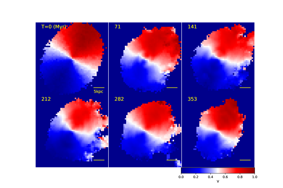
Figure 9: The same as Fig. 3 but for 2D gaseous kinematics (line-of-sight-velocity; $V_{\rm los}$).

4 Discussion

4.1 Further improvement

Although we have demonstrated that accurate predictions of the direction of galaxy motion with respect to ICM are possible ($\cos\Theta_{\rm m}=0.945$) for most models, we consider that further improvement on the predictions would be possible. We have so far focused exclusively on the predictions of galaxy motion with respect to ICM through CNNs trained by a large number of images of projected gaseous density, which is regarded as ‘mono-modal’ (one-channel) prediction. We here stress that more than one physical quantities of simulated galaxies under RPS can be fed into CNNs to have better accuracies in the new prediction methods. 2D stellar kinematics of gas in disk galaxies under RPS as well as 2D density map can be also used to train CNNs for the predictions. Such a ‘multi-modal’ prediction can improve the accuracy, because the 2D kinematics of gas in disk galaxies under RPS can be sensitive to the galaxy motions, as shown in this paper.

In order to discuss whether 2D kinematics can be useful for the inference of $\theta$ and $\phi$, we here derive the 2D velocity maps of simulated galaxies, as done for 2D density maps. We first divide the gas disk ($R\leq R_{\rm g}$) of a galaxy into $50\times 50$ small areas (meshes) and estimate the mean $V_{\rm los}$ at each mesh point. Therefore, the mean $V_{\rm los}$ at a mesh point ($i$, $j$) (denoted as $V_{i,j}$) is as follows:

$$V_{i,j}=\frac{1}{M_{i,j}}\sum_{k=1}^{N_{\it i,j}}m_{k}v_{k},$$ (10)

where $M_{i,j}$, $N_{i,j}$, $m_{k}$, $v_{k}$ are the total mass of gas particles in the mesh point ($i$, $j$), the total number of gas particles in the mesh, the mass of a gas particle, and the line-of-sight velocity of the particle, respectively. We also normalize the 2D data as done for 2D density maps as follows:

$$V_{i,j}^{\prime}=\frac{V_{i,j}-V_{\rm min}}{V_{\rm max}-V_{\rm min}},$$ (11)

where $V_{\rm min}$ and $V_{\rm max}$ are the minimum and maximum values of $V$ among the $50\times 50$ meshes in a model for a given projection. This normalization procedure is taken for each image at each time step. This procedure of normalization ensures that $V_{i,j}^{\prime}$ ranges from 0 to 1.

As shown in Fig. 9, 2D kinematic map of cold ISM shows a number of unique features during strong RPS phases ($T=71$, 141, and 282 Myr). Although the zero-velocity curve (indicated by white-colored meshes) is symmetric looks like an almost straight-line at $T=0$, it starts to bend at $T=71$ Myr during RPS. Such bending or “kink” in the zero-velocity curve of the 2D kinematic map can be clearly seen at $T=141$, 212, and 282 Myr in this model. Such an asymmetric zero-velocity curve can not be so clearly seen at $T=353$ Myr, when a fraction of ISM of the disk galaxy has been removed from the galaxy. Also, the 2D kinematic map shows a certain degree of randomness in the downstream side (i.e., right part of the disk galaxy) at $T=71$, 141, 212, and 282 Myr, which is caused by gas particles in the short tails (“tentacles”) being stripped by ram pressure. These characteristic gaseous kinematics seen only in some localized areas of disk galaxies can be also used to make multi-model prediction for $\theta$ and $\phi$.

One of other key issues in the new method is the less accurate predictions for galaxies with smaller $\theta$ ($\leq 30^{\circ}$). This could be overcome, if we use a much larger number of images $N_{i}>10^{5}$ constructed from models with smaller $\theta$. Although this is feasible for available (GPU) computing resources (to the author), it is a considerably time-consuming work both for the performance of the required simulations of galaxies under RPS (i.e., running a large number of models, $>10^{3}$) and for the CNN-training for a larger number of images. If the accuracy of CNN-based prediction for smaller $\theta$ is indeed improved by increasing $N_{\rm i}$ significantly, then the CNN can be practically applied to the observed galaxies in which any combination of $\theta$ and $\phi$ is possible. It is thus our future study to train a CNN with significantly larger $N_{\rm i}$. An alternative method to improve the accuracy of prediction for $\theta<30^{\circ}$ is to combine the present models used for training a CNN with many new models with $\theta<30^{\circ}$ and thereby to train a CNN again. At this point, it is not clear how many additional models for $\theta<30^{\circ}$ is required for the substantial improvement of predictability, and it is unclear whether this method does work to overcome the above-mentioned problem. However, it is doubtlessly worthwhile for our future studies to investigate this problem based on the above alternative method. If $\theta$ is better predicted in our future studies, then the developed CNN can be applied to real observational data with spatial resolutions similar to those adopted in the present study. Since gaseous distributions and kinematics of galaxies within clusters and groups are being investigated by the WALLABY project, our CNN will be able to be first applied for such gaseous data.

4.2 Constraining the 3D motion of galaxies under RPS

We have demonstrated that CNNs trained by synthesized images of simulated disk galaxies under RPS can determine $\theta$ and $\phi$ of the galaxies accurately. The next step is to apply the trained CNNs to real observational datasets. As shown in Fig. 10, the level of accuracy in the CNN-based prediction of $\theta$ and $\phi$ is not so much different between models with different spatial resolutions of $h_{\rm sm}=0.88$ kpc and 1.75 kpc. This implies that the direction of galaxy motion with respect to ICM can be inferred from 2D gas density maps of galaxies under RPS, if the spatial resolutions of the maps are as high as $\sim 1-2$ kpc. Such a required spatial resolution can be achieved for nearby groups of galaxies in the ongoing WALLABY H i (ASKAP HI All-Sky Survey; Koribalski et al. 2012) project with the spatial resolution of 30 arcsec for galaxies in groups and clusters. Since the spatial resolution for galaxies in the Fornax cluster is $\sim 3$ kpc in the WALLABY survey, it might be a bit difficult to determine $\theta$ and $\phi$ using the CNN trained in the present study. However, future observational studies of galaxies by the Square Kilometre Array (SKA) will be able to have much better spatial resolutions so that determination of $\theta$ and $\phi$ from observational datasets can be much more feasible not only for galaxies in nearby clusters (e.g., Virgo and Fornax) but also for those in distant clusters (Coma etc).

If $\theta$ and $\phi$ are determined for a disk galaxy under RPS in a cluster of galaxies, then the next question is as to whether the 3D motion of the galaxy with respect to the cluster’s center can be inferred. Since $\theta$ and $\phi$ are defined as inclination angles of the disk with respect to the relative velocity between the ICM and the galaxy, the 3D motion with respect to the cluster center can be inferred, only when the ICM is in hydrostatic equilibrium and thus not moving. Although this required condition of hydrostatic equilibrium is reasonable in dynamically relaxed clusters, such a condition would not be met in growing clusters through merging of other groups and clusters. We here consider that it is still useful to provide a method to convert $\theta$ and $\phi$ into the 3D motion in a Cartesian coordinate for a case where ICM is not moving. In the following discussion, we assume that the total velocity ($V_{0}$) of a disk galaxy under RPS in a cluster can be inferred from other observations of the cluster and a theoretical model of the gravitational potential for the cluster and (ii) the center of the Cartesian coordinate is coincident with the center of the cluster.

First, we have to find the direction of 3D motion of a disk galaxy with respect to the cluster center. Here we consider that the spin axis of the galaxy is inclined by $\theta_{\rm s}$ degree with respect to the $z$-axis and $\phi_{\rm s}$ is the angle between the $x$-axis and the projected spin vector onto the $x$-$y$ plane. These $\theta_{\rm s}$ and $\phi_{\rm s}$ can be easily calculated from the observed viewing angles, $\theta_{\rm v}$ and $\phi_{\rm v}$, owing to the adopted Cartesian coordinate. The direction of the 3D motion (u) in the cluster is therefore as follows:

$${\bf u}={\bf T}(\theta,\phi){\bf S}(\theta_{\rm s},\phi_{\rm s}){\bf z}$$ (12)

where u is the unit vector of the galaxy’s motion, T is the rotation matrix as a function $\theta$ and $\phi$, S is the rotation matrix as a function $\theta_{\rm s}$ and $\phi_{\rm s}$, and z is the unit vector of the $z$-axis (i.e., z=(0,0,1)). Here ${\bf S}(\theta_{\rm s},\phi_{\rm s}){\bf z}$ denotes the direction of the spin vector of the disk galaxy in the Cartesian coordinate. Accordingly, the 3D velocity vector (V) of the galaxy is as follows:

$${\bf V}=V_{0}{\bf u},$$ (13)

where $V_{0}$ is the total velocity of the galaxy.

Since this vector V is defined with respect to the cluster center, further calculations are required to derive the proper motion of the galaxy on the sky. Since the line-of-sight-velocity ($v_{\rm los}$) of the galaxy can be derived from spectroscopic observations, the tangential motion ($v_{\rm t}$) can be derived using the following equation:

$$V_{0}=\sqrt{v_{\rm los}^{2}+v_{\rm t}^{2}}.$$ (14)

The projected direction vector of the galaxy motion (${\bf u_{\rm g}}$) on the sky can be calculated by using the above vector u. This conversion from u to ${\bf u_{\rm g}}$ can be done in a straightforward manner. Using $v_{\rm t}$ and ${\bf u_{\rm g}}$, one can discuss the PM of the galaxy on the sky in principle. So far we have assumed that $V_{0}$ can be derived from other observations and theoretical models of the cluster. However, it is a formidable task to derive $V_{0}$ for a given projected distance of a galaxy from the center of its cluster, partly because the 3D position can not be derived in a straightforward manner. It is our future study to investigate whether we can simultaneously constrain $V_{0}$, $\theta$, and $\phi$ of a disk galaxy under RPS by applying CNNs to observations (under an assumption that $\rho_{\rm icm}$ can be constrained by other observations). If such simultaneous constraint is confirmed to be possible, then we can discuss the 3D motion of the galaxy in its host cluster without using results from other observations and gravitational potential models of the cluster.

Figure 10: The same as Fig. 5 but for models with different Gaussian smoothing lengths of $h_{\rm sm}=0.88$ kpc and 1.75 kpc. In these models, $\theta$ ($\phi$) ranges from $45^{\circ}$ ($30^{\circ}$) to $60^{\circ}$ ($60^{\circ}$).

5 Conclusion

We have adopted a convolutional neutral network (CNN) in order to infer the direction of 3D motion of a disk galaxy under RPS with respect to ICM of its host cluster based on the 2D gas density map of the galaxy. The present study is the very first step toward CNN-based very accurate predictions of 3D motion of galaxies under RPS. We have found that if the CNN is trained by $\sim 60000$ 2D density maps (images) produced by numerous RPS models, then the trained CNN can accurately predict the direction of galaxy motion. The mean cosine similarity between correct and predicted directions of galaxy motion in test models is $\cos\Theta_{\rm m}=0.95$ corresponding to $\Theta$ of $18.2^{\circ}$ (with $\cos\Theta_{\rm m}=1$ meaning perfect consistency between the two directions): the mean difference between predicted and correct vectors of galaxy motion is $\approx 18^{\circ}$. This is a promising result in this preliminary study, given that we did not fully explore the sets of model parameters that control the strength of RPS, the masses of clusters, and the types of galaxies.

However, the trained CNN can not so accurately ($\cos\Theta_{\rm m}\sim 0.85$ corresponding to $\Theta 32^{\circ}$) predict the direction of 3D motion of galaxies for a certain range of angles ($\theta$ and $\phi$) between the spin axes of galaxies under RPS and the direction of 3D motion of the galaxies. This problem will need to be overcome in our future study so that the 3D motion of galaxies can be precisely predicted for any $\theta$ and $\phi$ of the 3D motion of the galaxies. Once this problem is fixed, then we can try to drive the 3D motion of galaxies with respect to the center of their host cluster by adopting an assumption that ICM is in hydrostatic equilibrium and thus not moving with respect to the cluster center. Such an assumption of static ICM may be true only for dynamically relaxed clusters without merging of sub-clusters.

If the 3D orbits (e.g., orbital eccentricities) for an enough number of disk galaxies can be well constrained by the method presented in this paper, they can be used to discuss whether the orbit of a disk galaxy can be correlated with (i) their morphological properties (e.g., S0s in more radial orbits ?), (ii) star formation histories (e.g., more likely to have been quenched in small pericenter distances ?), and the 2D distributions of star-forming regions (e.g., peculiar distributions of H$\alpha$ emission in infalling galaxy populations ?). Also they can be used to discuss the orbital properties of cluster member galaxies predicted from $\Lambda$CDM models (e.g., Ghigna et al. 1998). Accordingly, constraining the 3D orbits of cluster member galaxies can have important implications on the cosmological models of galaxy formation. It is thus our future study to improve greatly the accuracy of prediction on $\theta$ and $\phi$ for disk galaxies under RPS in cluster environments.

6 Acknowledgment

I (Kenji Bekki; KB) am grateful to the referee for constructive and useful comments that improved this paper.

Appendix A CNN-based determination of directions vectors

Fig. A1 briefly describes the adopted CNN architecture and the basic method to determine the 3D motion of a disk galaxy under RPS (i.e., determination of $\theta$ and $\phi$). There are only two differences in the adopted CNN between the present study and Stanley & Bekki (2018). One is the mesh sizes of the input layer: $50\times 50$ in the present study and $20\times 20$ in SB18. The other is the activation function in the final layer: liner function in the present study and softmax one in SB18. We have only discussed the CNN-based training and testing phases of simulated 2D images of disk galaxies, not the observed ones in the present study. As discussed in Bekki et al. (2018), the application of CNNs trained by simulations dataset is not so simple owing to a number of observational factors such as observational errors and different resolutions between observations and simulations. These are beyond the scope of this paper and will be discussed in our future papers.

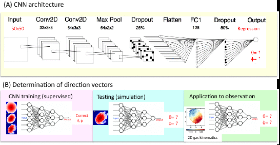
Figure 11: Illustration of the adopted CNN architecture and the basic method to determine the direction vector of the 3D motion ($\theta$ and $\phi$) of a disk galaxy under RPS based on the training CNN. The details of the method is given in the main text. This figure is produced by using figures from Nathan & Bekki (2018) and galaxy images from the SAMI survey (e.g., Croom et al. 2014).

Appendix B Consistency check for $\theta$ and $\phi$

Although $\cos\Theta$ is a good way to measure the level of consistency between predicted and correct directions of galaxy motion (with respect to ICM motion), it is instructive to show how accurately the trained CNN can predict $\theta$ and $\phi$ separately. Fig. B1 describes the predicted angles ($\theta_{\rm p}$ and $\phi_{\rm p}$) as a function of correct ones ($\theta_{\rm c}$ and $\phi_{\rm c}$) for selected 6000 models. For each of the selected $\theta$, the results for 10 different $\phi$ are shown in this figure. Clearly, the trained CNN can predict the two angles well, though the prediction is not so precise for a given $\theta$: some models shows significant deviation from correct $\theta$. (Our initial expectation was that the CNN can less accurately predict $\phi$). The level of these deviation of predicted $\theta$ and $\phi$ is found to be similar between different sets of models (T0-T9). A possible way to solve this problem is discussed in the main text (§4).

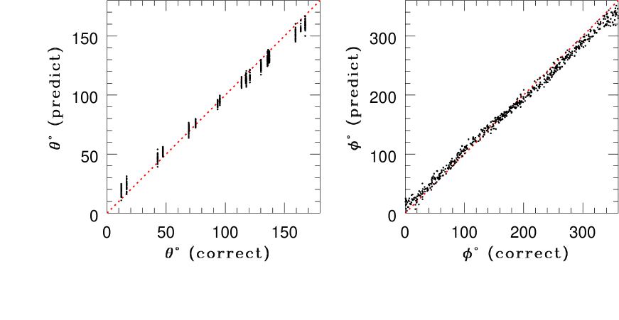
Figure 12: The predicted and correct $\theta$ (left) and $\phi$ (right) for the selected 6000 models. The red dotted lines indicate $\theta_{\rm p}=\theta_{\rm c}$ (left) and $\phi_{\rm p}=\phi_{\rm c}$ (right).

Appendix C The mass-ratio of ICM to ISM particles

It is instructive for this study to show the time evolution of the mass-ratio ($r_{\rm m}$) of ICM particle ($m_{\rm ICM}$) to ISM particle ($m_{\rm g}$), because $r_{\rm m}$ can influence significantly the RPS processes (in particular, for very large $r_{\rm m}$). Fig. C1 shows the time evolution of $r_{\rm m}$ for $\sim 0.28$ Gyr in the fiducial model. The masses of ISM particles in a galaxy can change with time owing to gas ejection from SNe and AGB stars, and the change rates are different between different particles (owing to the different chemical enrichment histories between different gas particles). Therefore we estimate the mean of $m_{\rm g}$ at each time step in order to estimate $r_{\rm m}$. The initial masses of ICM and ISM particles are $1.7\times 10^{5}{\rm M}_{\odot}$ and $3.0\times 10^{5}{\rm M}_{\odot}$, respectively. As the spiral galaxy moves into the core of the Coma cluster model, $r_{\rm m}$ can increase owing to the increase of the ICM density. However, $r_{\rm m}$ can be kept lower, i.e., $<2$, which confirms that gas stripping due to large $r_{\rm m}$ (i.e., numerical artifact) can be avoided in the present RPS model using a cubic box. Owing to gas ejection of Type II SNe, gas particles very close to such SNII can increase $m_{\rm g}$ only slightly during a simulation. Therefore, $m_{\rm g}$ can be regarded as being almost constant when it comes to the discussion on $m_{\rm ICM}/m_{\rm g}$ evolution here.

Figure 13: Time evolution of the mass-ratio ($r_{\rm m}$) of ICM particle ($m_{\rm ICM}$) to ISM particle ($m_{\rm g}$) in the fiducial model.

References

- (1) Abadi, M. G., Moore, B., Bower, R. G., 1999, MNRAS, 308, 947
- (2) Bekki, K. 2009, MNRAS, 399, 2221
- (3) Bekki, K., 2013, MNRAS, 432, 2298 (B13)
- (4) Bekki, K., 2014, MNRAS, 438, 444 (B14)
- (5) Bekki, K., 2015, MNRAS, 449, 1625
- (6) Bekki, K., Couch, W. J., 2003, ApJ, 596, L13
- (7) Boselli, A., Gavazzi, G., 2006, PASP, 118, 517
- (8) Cortese, K., et al., 2016, MNRAS, 459, 3574
- (9) Crowl, H. H., Kenney, J. D. P., 2008, AJ, 136, 1623
- (10) Dieleman, S., Willett, K. W., Dambre, J., 2015, MNRAS, 450, 1441
- (11) Dominguez Sanchez, H., Huertas-Company, M., Bernardi, M., Tuccillo, D., Fischer, J. L., 2018, MNRAS, in press
- (12) Henderson, B., Bekki, K., 2016, ApJ, 822, L33
- (13) Ghigna, S., Moore, B., Governato, F., Lake, G., Quinn, T., Stadel, J., 1998, MNRAS, 300, 146
- (14) Gunn, J. E., Gott, J. R. III., 1972, ApJ, 176, 1
- (15) Jáchym, P., et al., 2017, ApJ, 839, 114
- (16) Kawata, D., Mulchaey, J. S., 2008, ApJ, 672, L103
- (17) Kenney, J. D. P., Abramson, A., Bravo-Alfaro, H., 2015, AJ, 150, 59
- (18) Kennicutt, R. C. 1998, ApJ, 498, 541
- (19) Chollet, F., 2015, https://keras.io/
-
(20)
Koribalski et al. 2012, http://www.atnf.csiro.au/
research/WALLABY/ - (21) Kronberger, T., Kapferer, W., Ferrari, C., Unterguggenberger, S., Schindler, S., 2008, A&A, 481, 337
- (22) Larson, R. B., Tinsley, B. M., Caldwell, C. N., 1980, ApJ, 237, 692
- (23) McCarthy, I. G., Frenk, C. S., Font, A. S., Lacey, C. G., Bower, R. G., Mitchell, N. L., Balogh, M. L., Theuns, T., 2008, MNRAS, 383, 593
- (24) Matsumoto, H., Tsuru, T. G., Fukazawa, Y., Hattori, M., Davis, D. S., 2000, PASJ, 52, 153
- (25) Navarro, J. F., Frenk, C. S., White, S. D. M., 1996, ApJ, 462, 563 (NFW)
- (26) Neto, A. F., 2007, MNRAS, 381, 1450
- (27) Quilis, V., Moore, B., Bower, R., 2000, Sci, 288, 1617
- (28) Roediger, E., Hensler, G., 2005, A&A, 433, 875
- (29) Singhal, A., 2001, Bulletin of the IEEE Computer Society Technical Committee on Data Engineering, 24, 35
- (30) Stanley, N., Bekki, K., in prepartion (SB18)
- (31) Tonnesen, S., Bryan, G. L., 2012, MNRAS, 422, 1609
- (32) Vollmer, B., Cayatte, V., Balkowski, C., Duschl, W. J., 2001, ApJ, 561, 708
- (33) Wong, O. I., Kenney, J. D. P., Murphy, E. J., Helou, G., 2014, ApJ, 783, 109
- (34) Zeiler, M. D., astro-ph/arXiv:1212.5701