Approximate Curve-Restricted Simplification of Polygonal Curves

Abstract

The goal in the min-# curve simplification problem is to reduce the number of the vertices of a polygonal curve without changing its shape significantly. We study curve-restricted min-# simplification of polygonal curves, in which the vertices of the simplified curve can be placed on any point of the input curve, provided that they respect the order along that curve. For local directed Hausdorff distance from the input to the simplified curve in $\mathbb{R}^{2}$, we present an approximation algorithm that computes a curve whose number of links is at most twice the minimum possible.

Keywords: Curve simplification, geometric algorithms, computational geometry.

2010 Mathematics subject classification: 68U05.

1 Introduction

The goal of the classical curve simplification problem is to reduce the number of the vertices of a polygonal curve, without changing its shape significantly. There are several applications in which curve simplification plays an important role. In trajectory analysis, for instance, there are two important reasons for this reduction. First, it reduces the storage and bandwidth requirements for storing and transferring huge and growing collections of trajectory data. Second, and probably more importantly, the complexity of most trajectory analysis algorithms depends on the number of the vertices of the input curves, and simplifying trajectories can reduce the running time of these algorithms.

Let $P=\left<p_{1},p_{2},...,p_{n}\right>$ be a polygonal curve on the plane. The curve $P^{\prime}=\left<p^{\prime}_{1},p^{\prime}_{2},...,p^{\prime}_{m}\right>$ is a simplification of $P$, if $p^{\prime}_{1}=p_{1}$, $p^{\prime}_{m}=p_{n}$, $m\leq n$, and the distance between $P$ and $P^{\prime}$ is at most $\epsilon$ (the definition of the distance between these curves and the value of $\epsilon$ is described below). The simplified curve may be vertex-restricted, curve-restricted, or unrestricted. In vertex-restricted simplification, the vertices of $P^{\prime}$ coincide with the vertices of the input curve, i.e. for each $i$ where $1\leq i\leq m$, $p^{\prime}_{i}=p_{j}$ for some index $j$, where $1\leq j\leq n$. In curve-restricted simplification, the vertices of $P^{\prime}$ can be placed on any point of the input curve, and in unrestricted simplification there is no limitation on the placement of the internal vertices of $P^{\prime}$. In the first two cases, which is the focus of the present paper, the vertices of the simplified curve should appear in order on the input curve, and thus split $P$ into sub-curves. For each edge of the simplification $p^{\prime}_{i}p^{\prime}_{i+1}$, in which $1\leq i\leq m-1$, let $P_{p^{\prime}_{i}p^{\prime}_{i+1}}$ denote the sub-curve of $P$ from $p^{\prime}_{i}$ to $p^{\prime}_{i+1}$.

The distance between two curves is computed using measures such as Fréchet or Hausdorff [1] (other measures too are sometimes used such as [2]). Let $D(C,C^{\prime})$ denote the function that computes the distance between two curves using any such measure. The distance between the original and simplified curves is either global and computed for the curves as a whole, or is local and computed as the maximum distance of the corresponding sub-curves, i.e. $\max_{1\leq i\leq m-1}D(p^{\prime}_{i}p^{\prime}_{i+1},P_{p^{\prime}_{i}p^{\prime}_{i+1}})$.

Curve simplification is usually studied in two settings [3]. In the min-$\epsilon$ setting the maximum value of $m$ (the number of the vertices of the simplified curve) is specified and $\epsilon$ (the amount of distance between the original and simplified curves) is minimised, and in the min-# setting $\epsilon$ is given while $m$ is minimised. There are numerous results on vertex-restricted curve simplification in the min-# setting, only some of which provide a guarantee on the number of the vertices of the simplification. In the rest of this paper we focus on the min-# problem, and assume that $\epsilon$ is specified as an input.

The well-known algorithm presented by Douglas and Peucker [4] does not minimise the number of the vertices of the simplified curve, but is both simple and effective. It assumes local directed Hausdorff distance from the input curve to the simplified curve. For simplifying $P$ with the maximum distance $\epsilon$, it finds the most distant vertex $p_{k}$ from segment $p_{1}p_{n}$; if their distance is at most $\epsilon$, this segment is a link of the simplification. Otherwise, the algorithm recursively simplifies $\left<p_{1},...,p_{k}\right>$ and $\left<p_{k},...,p_{n}\right>$. The worst-case time complexity of this algorithm is $O(n^{2})$. Hershberger and Snoeyink [5, 6] improved the running time of this algorithm to $O(n\log n)$ and later to $O(n\log^{*}n)$.

Among algorithms that compute an optimal simplification, i.e. a simplification with the minimum number of links, the one presented by Imai and Iri [7] is probably the most popular for local Hausdorff distance. It creates a shortcut graph, the vertices of which represent the vertices of the input curve. An edge $p_{i}p_{j}$ shows that the distance between link $p_{i}p_{j}$ and sub-curve $\left<p_{i},p_{i+1},...,p_{j}\right>$ is at most $\epsilon$. A shortest path algorithm on this graph, finds the simplification with the minimum number of vertices. The time complexity of this algorithm is $O(n^{2}\log n)$. Chan and Chin [8], and also Melkman and O’Rourke [9] improved the running time of this algorithm to $O(n^{2})$, and Chen and Daescu [10] reduced its space complexity to $O(n)$.

There are many other results on vertex-restricted simplification that consider the Fréchet distance or compute the distance of the curves globally. For instance, van Kreveld at al. [11] studied the performance of the Douglas and Peucker [4] and Imai and Iri [7] algorithms, described above, under the global Hausdorff or Fréchet distance measures. They showed that computing an optimal vertex-restricted simplification using the global undirected Hausdorff distance or global directed Hausdorff distance from the simplified to the optimal curve is NP-hard, and presented an output-sensitive dynamic programming algorithm with the time complexity $O(mn^{5})$ for computing an optimal simplification under the global Fréchet distance. A faster dynamic programming algorithm for the same variation of the problem was presented by van de Kerkhof et al. [12] with the time complexity $O(n^{4})$.

Some results on vertex-restricted simplification do not obtain an optimal simplification but provide a guarantee on the number of the links of the resulting simplifications using approximation algorithms. Agarwal et al. [1] for instance, presented a near-linear time approximation algorithm for local Hausdorff distance using the uniform distance metric, in which the distance between a point and a curve is defined as their vertical distance. They also presented an approximation algorithm for local Fréchet distance under $L_{p}$ metric. Both of these algorithms are simple and greedy in nature. Among these results, there are also vertex-restricted simplification algorithms that assume streaming input or online setting [13, 14, 15, 16], in which a limited storage is available or the curve should be simplified in one pass. It is beyond the scope of this paper to review the literature on curve simplification extensively; even many heuristic algorithms, such as [17, 18], have been presented for curve simplification (Zhang et al. [19] surveyed many of them for trajectory simplification).

Despite the number of results on vertex-restricted curve simplification, curve-restricted simplification, which has attracted less attention, can yield a curve with much fewer vertices, as in Figure 1, in which a curve-restricted simplification with only four vertices is demonstrated for a curve whose vertex-restricted simplification is the same as the input curve. For global directed Hausdorff distance, van de Kerkhof et al. [12] showed that curve-restricted simplification is NP-hard and provided an $O(n)$ algorithm for global Fréchet distance in $\mathbb{R}^{1}$.

Figure 1: An example showing that curve-restricted simplifications can have far fewer vertices compared to vertex-restricted simplifications; the dashed links are a curve-restricted simplification of the curve with solid edges.

In this paper, we study the min-# curve-restricted simplification problem with maximum local Hausdorff distance $\epsilon$ from the input curve to the simplified curve. We present a dynamic programming algorithm that computes a simplified curve, the number of the links of which is at most twice the minimum possible. This paper is organized as follows: In Section 2 we introduce the notation used in this paper. In Section 3, we show how to compute a simplification link between two edges of the input curve and in Section 4, we present our main algorithm. We conclude this paper Section 5.

2 Preliminaries and Notation

A two-dimensional polygonal curve is represented as a sequence of vertices on the plane, with line segments as edges between contiguous vertices. The directed Hausdorff distance between curves $C$ and $C^{\prime}$, denoted as $H(C,C^{\prime})$, is defined as the maximum of the distance between any point of $C$ to the curve $C^{\prime}$, i.e. $H(C,C^{\prime})=\max_{p\in C}\mathit{dist}(p,C^{\prime})$, in which $\mathit{dist}(p,C^{\prime})$ is the Euclidean distance between point $p$ and curve $C^{\prime}$.

Let $P^{\prime}=\left<p^{\prime}_{1},p^{\prime}_{2},...,p^{\prime}_{m}\right>$ be a curve-restricted simplification of $P$. We have $p^{\prime}_{1}=p_{1}$, $p^{\prime}_{m}=p_{n}$, $m\leq n$, and the distance between $P$ and $P^{\prime}$ is at most $\epsilon$. Also, the vertices of $P^{\prime}$ should appear in order along $P$. Given a parameter $\epsilon$, the goal in the min-# simplification is to find a simplified curve with the minimum number of vertices, such that the distance between the original and simplified curves is at most $\epsilon$. In what follows, we use the term link to refer to the edges of the simplified curve, to distinguish them from the edges of the input curve.

For a link $\ell$ of $P^{\prime}$, suppose $x$ and $y$ on $P$ are points corresponding to the start and end points of $\ell$ and suppose $x$ is on edge $p_{i}p_{i+1}$ and $y$ is on $p_{j}p_{j+1}$. Then, $\ell$ covers all edges $p_{k}p_{k+1}$ for $i\leq k\leq j$. Let $P_{\ell}$ be the sub-curve of $P$ corresponding to link $\ell$, i.e. the sub-curve of $P$ from point $x$ to $y$. The local Hausdorff distance from $P$ to $P^{\prime}$ is the maximum of $H(P_{\ell},\ell)$ over all links $\ell$ of $P^{\prime}$. In this paper we assume local Hausdorff distance to measure the distance between the input and simplified curves.

The $\epsilon$-neighbourhood of a vertex of $P$ or a segment which is defined as follows.

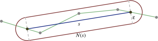
Figure 2: The $\epsilon$ neighbourhood of a segment

Definition 2.1.

The $\epsilon$-neighbourhood of a point $p$, denoted as $N(p)$ is a disk of radius $\epsilon$ and with centre is at $p$. Clearly, the set of points inside $N(p)$ are all points at distance at most $\epsilon$ from $p$. Similarly, the $\epsilon$-neighbourhood of a segment $s$, denoted as $N(s)$, is the set of points at distance at most $\epsilon$ from any point of the segment $s$.

The $\epsilon$-neighbourhood of a segment $s$ is demonstrated in Figure 2.

3 Identifying Simplification Links

Lemma 3.1.

For the curve $P=\left<p_{1},p_{2},...,p_{n}\right>$, a segment $s$ from point $x$ on edge $p_{i}p_{i+1}$ to point $y$ on edge $p_{j}p_{j+1}$ can be a link of a (not necessarily optimal) curve-restricted simplification if and only if it intersects $N(p_{k})$ for every index $k$, where $i<k\leq j$.

Proof.

Let $C$ be the sub-curve $P$ from $x$ to $y$. If $s$ is a link of a simplification of $P$, $H(C,s)$ is at most $\epsilon$. This implies that the distance of every point of $C$ to $s$ is at most $\epsilon$. For each vertex $p$ of $C$ this means that $s$ should include at least one point from $N(p)$.

For the converse, suppose $s$ intersects $p_{i}p_{i+1}$ at $x$ and $p_{j}p_{j+1}$ at $y$, as well as $N(p)$ for every vertex of $C$, the sub-curve of $P$ from $x$ to $y$. It is enough to show that $H(C,s)\leq\epsilon$. For each edge, since the distance between its end points and $s$ is at most $\epsilon$, the distance of other points of the edge cannot be greater. This holds for every internal edge of $C$ and implies $H(C,s)\leq\epsilon$ as required. ∎

Lemma 3.1 corresponds to a similar statement for vertex-restricted simplifications. We use this lemma later to compute the links of a simplification.

Corollary 3.2.

For the curve $P=\left<p_{1},p_{2},...,p_{n}\right>$, a segment $s$ from point $x$ on edge $p_{i}p_{i+1}$ to point $y$ on edge $p_{j}p_{j+1}$ is a link of a (not necessarily optimal) curve-restricted simplification if and only if $N(s)$ contains $p_{k}$ for every index $k$, where $i<k\leq j$.

Corollary 3.2 holds because if a segment $s$ intersects the $\epsilon$-neighbourhood of a vertex $v_{k}$, the distance of $v_{k}$ to $s$ is at most $\epsilon$ and it should be inside $N(s)$. We use Corollary 3.2 later to improve the time complexity of detecting simplification links.

Lemma 3.3.

Suppose $\ell$ is a link of a curve-restricted simplification of curve $P=\left<p_{1},p_{2},...,p_{n}\right>$, such that $\ell$ starts from point $x$ on edge $p_{i}p_{i+1}$ and ends at point $y$ on edge $p_{j}p_{j+1}$. There exists another link $\ell^{\prime}$ covering the same set of edges such that the line that results from extending $\ell^{\prime}$ has the following property for at least two values of $k$ where $i<k\leq j$: either i) it is a tangent to $N(p_{k})$, or ii) it passes through one of the end points of $p_{i}p_{i+1}$ or $p_{j}p_{j+1}$, or their intersection with $N(p_{k})$.

Proof.

Let $L$ be the line resulting from extending the segment $\ell$. If none of the mentioned properties hold for any value of $k$, we move $L$ downwards until one of them holds for some value $k$, i.e. it becomes tangent to the $\epsilon$-neighbourhood of $p_{k}$ or passes through the intersection of the $\epsilon$-neighbourhood of $p_{k}$ and the last or the first edge covered by the $s$. We then rotate $L$ around $p_{k}$ for case i, or the intersection of case ii, until one of the conditions holds for another index. Let $s$ be the segment on line $L$ with end points on $p_{i}p_{i+1}$ and $p_{j}p_{j+1}$; such a segment surely exist, since the movement or rotation stops at the end points of these edges.

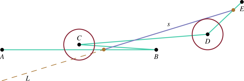
Figure 3: Rotating line $L$ around $N(D)$ counterclockwise; $s$ no longer intersects $N(C)$.

Clearly $L$ cannot leave $N(p_{k})$ for any possible index $k$ for both the downward movement and the rotation; just before leaving $N(p_{k})$, $L$ becomes its tangent. The only problem may be that although $N(p_{k})$, for some $k$ where $i<k\leq j$, is intersected by both $\ell$ and $L$, $s$ may be too short to intersect $N(p_{k})$; this is demonstrated in Figure 3. However, since the rotation stops at the intersection the first or the last edge and $N(p_{k})$, this case never happens. ∎

Lemma 3.4.

A link of a curve-restricted simplification of $P=\left<p_{1},p_{2},...,p_{n}\right>$, from a point on edge $p_{i}p_{i+1}$ to a point on edge $p_{j}p_{j+1}$ can be found with the time complexity $O(m^{3})$ where $m=j-i+1$, provided such a link exists.

Proof.

We find a line for which the condition mentioned in Lemma 3.3 holds. To do so, we find three parallel lines at distance $\epsilon$ on the plane, $L_{1}$, $L_{2}$, and $L_{3}$, such that a link can be found on line $L_{2}$. We consider possible placements of these lines according to Lemma 3.3 and check for which of them the condition of Lemma 3.1 holds for a segment on $L_{2}$. If $L_{2}$ is a tangent to $N(p_{k})$ for some value of $k$ where $i<k\leq j$, then either $L_{1}$ or $L_{3}$ should pass through $p_{k}$. We therefore try different placements of these three lines such that the following property holds for two values of $k$ for $i<k\leq j$: either i) $L_{1}$ or $L_{3}$ passes through $p_{k}$, or ii) $L_{2}$ passes through the intersection $N(p_{k})$ and one of $p_{i-1}p_{i}$ or $p_{j}p_{j+1}$ or the end points of these edges. Since there are $O(m)$ choices for the first and the second conditions, the number of total cases to consider is $O(m^{2})$.

For each of $O(n^{2})$ possible placements of these lines, we have to verify if there exists a segment $s$ on $L_{2}$ such that $H(C,s)$ is at most $\epsilon$. Let $x$ be the intersection of $L_{2}$ and $p_{i}p_{i+1}$ and let $y$ be the intersection of $L_{2}$ and $p_{j}p_{j+1}$; if $x$ or $y$ do not exist, $L_{2}$ cannot contain a link. Based on Lemma 3.1, if the segment $xy$ intersects $N(p_{k})$ for every $i<k\leq j$, it is a valid link. This can be checked with the time complexity $O(m)$. ∎

Corollary 3.5.

To force the link to start from $p_{i}$, instead of any point on edge $p_{i}p_{i+1}$ in Lemma 3.4, we can fix this point on $L_{2}$ and try the condition mentioned in the proof of Lemma 3.4 for only one value of $k$.

Algorithms based on the construction of the shortcut graph of Imai and Iri [7] perform steps similar to Lemma 3.4: for each $i$ and $j$, where $1\leq i<j\leq n$, it should be verified if the segment $p_{i}p_{j}$ intersects the $\epsilon$-neighbourhood of every vertex $p_{k}$ for $i<k<j$. This task can be optimised by computing the set of lines that pass through $p_{i}$ and intersect the $\epsilon$-neighbourhood of the vertices that appear after it (the intersection of double cones; see [10], for instance). Unfortunately, for curve-restricted simplification that does not seem possible, since the end points of each link may not be a vertex and are chosen from a much larger set (see Lemma 3.3). Therefore, to improve the time complexity of Lemma 3.4, we should use an alternative strategy.

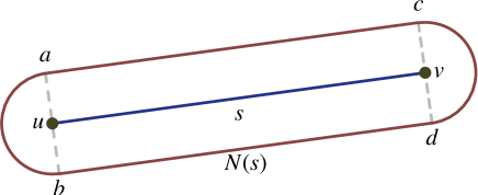
Figure 4: Symbols used for $N(s)$ in Lemma 3.6

Lemma 3.6.

Let $S$ be a set of $n$ points on the plane and let $\delta$ be a constant, where $0<\delta<1$. There exists a data structure with $O(n^{1+\delta})$ preprocessing time and space, which, for any segment $s$, can verify if all points in $S$ are inside the $\epsilon$-neighbourhood of $s$ in $O(2^{1/\delta}\log n)$ time.

Proof.

We first compute the convex hull $H$ of the points in $S$. The most distant point of $S$ from $s$ is a vertex of $H$. Let $\ell(x,y)$ be the line that results from extending the segment from point $x$ to point $y$, and let $h(x,y)$ be the halfplane on the left side of $\ell(x,y)$. All members of $S$ are in $N(s)$, if and only if there is no point in the following four regions (we use the symbols defined in Figure 4):

1. $h(a,c)$,

2. $h(d,b)$,

3. $h(b,a)\setminus N(u)$, and

4. $h(c,d)\setminus N(u)$.

Since, the intersections of a convex polygon and a line can be computed in logarithmic time, the first two regions can be checked in $O(\log n)$. The other two regions can be checked using halfplane proximity queries: given a directed line $\ell$ and a point $q$, report the point farthest from $q$ among those to the left of $\ell$. Aronov et al. [20] presented a data structure that uses $O(n^{1+\delta})$ preprocessing time and space, to answer such queries in $O(2^{1/\delta}\log n)$ time, for any $\delta$ ($0<\delta<1$). Therefore, to check the third region, we perform a halfplane proximity query for line $\ell(b,a)$ and point $u$; only if the distance of the farthest point to $u$ in $h(b,a)$ is at most $\epsilon$, the third region is empty. Similarly, to check the fourth region, we perform a halfplane proximity query, specifying line $\ell(c,d)$ and point $v$ as inputs. ∎

Lemma 3.7.

Let $\delta$ be a constant, where $0<\delta<1$. With $O(n^{3+\delta})$ preprocessing time and space, a link of a curve-restricted simplification of a polygonal curve $P=\left<p_{1},p_{2},...,p_{n}\right>$, from any edge $p_{i}p_{i+1}$ to any other edge $p_{j}p_{j+1}$ can be found with the time complexity $O(n^{2}\log n)$, provided that such a link exists.

Proof.

For every pair of indices $x$ and $y$, where $1<x\leq y<n$, we initialize the data structure mentioned in Lemma 3.6 $D_{xy}$ for points $\{p_{x},p_{x+1},...,p_{y}\}$. This can be done with the time complexity $O(n^{3+\delta})$. In Lemma 3.4, to check if a segment from $p_{i}p_{i+1}$ to $p_{j}p_{j+1}$ is a link, we test to see if it intersects $N(p_{k})$ for every index $k$, where $i<k\leq j$. We improve the time complexity of this task to $O(\log n)$ by using $D_{xy}$. ∎

4 Simplification Algorithm

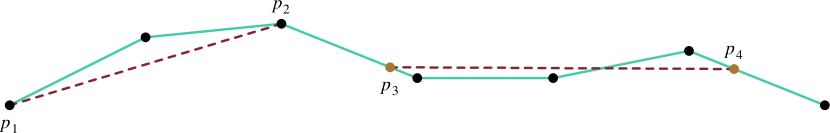
Figure 5: A DLC $\left<p^{\prime}_{1}p^{\prime}_{2},p^{\prime}_{3}p^{\prime}_{4}\right>$ of a curve with six links (Definition 4.1)

Definition 4.1.

A sequence of segments $D=\left<p^{\prime}_{1}p^{\prime}_{2},p^{\prime}_{3}p^{\prime}_{4},...,p^{\prime}_{2k-1}p^{\prime}_{2k}\right>$ is a disjoint link chain (DLC) for curve $P=\left<p_{1},p_{2},...,p_{n}\right>$, if i) $p^{\prime}_{1}$ is on $p_{1}p_{2}$ and $p^{\prime}_{2k}$ is on $p_{n-1}p_{n}$, ii) for each index $i$, where $1\leq i\leq k$, $p^{\prime}_{2i-1}p^{\prime}_{2i}$ is a valid simplification link, and iii) for each index $i$, where $1\leq i<k$, $p^{\prime}_{2i}$ and $p^{\prime}_{2i+1}$ are on the same edge of $P$, and iv) the vertices of $D$ appear in order on $P$ (i.e. first $p^{\prime}_{1}$ appears on $P$, then $p^{\prime}_{2}$, then $p^{\prime}_{3}$, and so forth).

Figure 5 demonstrates a DLC of a curve with six links.

Proposition 4.2.

Given a DLC $D=\left<p^{\prime}_{1}p^{\prime}_{2},p^{\prime}_{3}p^{\prime}_{4},...,p^{\prime}_{2k-1}p^{\prime}_{2k}\right>$ for curve $P=\left<p_{1},p_{2},...,p_{n}\right>$, such that $p^{\prime}_{1}=p_{1}$, a curve-restricted simplification of $P$ with $2k$ links can be obtained from $D$ by connecting the end of each link of $D$ to the start of its next link and connecting the end of the last one to $p_{n}$.

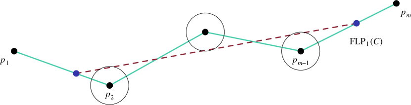
Figure 6: $\mathrm{FLP}_{1}(\left<p_{1},p_{2},...,p_{m}\right>)$ of a curve with six links (Definition 4.3)

Definition 4.3.

For a polygonal curve $C=\left<p_{1},p_{2},...,p_{m}\right>$, the first link point with $k$ links, denoted as $\mathrm{FLP}_{k}(C)$, is the first point $x$ on $p_{m-1}p_{m}$, such that there exists a disjoint link chain $D=\left<p^{\prime}_{1}p^{\prime}_{2},p^{\prime}_{3}p^{\prime}_{4},...,p^{\prime}_{2k-1}p^{\prime}_{2k}\right>$ of $C$, in which $p^{\prime}_{2k}=x$.

Figure 6 demonstrates $\mathrm{FLP}_{1}$ of a curve with four edges. Since the line containing a link can be moved or rotated to obtain a new link, unless the conditions mentioned in Lemma 3.3 holds for it, Lemma 3.7 yields the following corollary.

Corollary 4.4.

For a sub-curve $Q=\left<q_{1},q_{2},...,q_{m}\right>$ of a polygonal curve $P=\left<p_{1},p_{2},...,p_{n}\right>$, $\mathrm{FLP}_{1}(Q)$ and its corresponding link can be computed with the time complexity $O(n^{2}\log n)$, after some preprocessing with the time complexity $O(n^{3+\delta})$, for some constant $\delta$ ($0<\delta<1$).

In Theorem 4.5 we present an algorithm for computing a minimum-sized DLC.

Theorem 4.5.

A DLC of minimum size for curve $P=\left<p_{1},p_{2},...,p_{n}\right>$ can be computed in $O(n^{5}\log n)$.

Proof.

We use dynamic programming to fill a two-dimensional table $F$. $F[i,j]$, for $1\leq i\leq n$ and $1\leq j\leq n$, denotes $\mathrm{FLP}_{j}(\left<p_{1},p_{2},...,p_{i}\right>)$. Parallel to table $F$, we can store the last link of $F[i,j]$ in another two-dimensional table $L$ to reconstruct the chain. For points $u$ and $v$ on $P$, $u<v$ holds if $u$ appears before $v$ on $P$. We fill the tables as follows.

1. $F[i][1]$ is initialized as $\mathrm{FLP}_{1}(\left<p_{1},p_{2},...,p_{i}\right>)$, forcing the first vertex of the resulting link to be on $p_{1}$ (Corollary 3.5). $L[i][1]$ is initialised as the link corresponding to $\mathrm{FLP}_{1}(\left<p_{1},p_{2},...,p_{i}\right>)$. If there is no such link, $F[i][1]$ and $L[i][1]$ are not filled.

2. For $d$ from $2$ to $n$, $F[i][d]$ and $L[i][d]$ for $1\leq i\leq n$ are filled as follows: The value $F[i][d]$ is the minimum value of $\mathrm{FLT}_{1}(\left<F[j][d-1],p_{j+1},p_{j+2},...,p_{i}\right>)$, over all indices of $j$, where $j<i$ and $F[j][d-1]$ is filled. The value of $L[i][d]$ should indicate the link corresponding to of $\mathrm{FLT}_{1}(\left<F[j][d-1],p_{j+1},p_{j+2},...,p_{i}\right>)$.

Based on Corollary 4.4, filling these tables can be done with the time complexity $O(n^{5}\log n)$.

Let $m$ be the lowest index, such that $F[n][m]$ is filled. By following the links backwards using dynamic programming tables, we obtain a DLC $D=\left<p^{\prime}_{1}p^{\prime}_{2},p^{\prime}_{3}p^{\prime}_{4},...,p^{\prime}_{2k-1}p^{\prime}_{2k}\right>$. We prove that the size of $D$ is the minimum possible. To do so, we use induction on $d$ to show that $F[i][d]$ for $1\leq i\leq n$ is filled if and only if there is a DLC for $\left<p_{1},p_{2},...,p_{i}\right>$ with $d$ links. For $d=1$, the statement is trivial and follows from the definition of $\mathrm{FLT}_{1}$ and its computation (Corollary 3.5). For $d>1$, suppose there is a DLC $\left<q^{\prime}_{1}q^{\prime}_{2},q^{\prime}_{3}q^{\prime}_{4},...,q^{\prime}_{2d-1}q^{\prime}_{2d}\right>$ for $\left<p_{1},p_{2},...,p_{i}\right>$. Let $q^{\prime}_{2d-2}$ be on $p_{j}p_{j+1}$. Obviously, $\left<q^{\prime}_{1}q^{\prime}_{2},q^{\prime}_{3}q^{\prime}_{4},...,q^{\prime}_{2d-3}q^{\prime}_{2d-2}\right>$ is a DLC of $\left<p_{1},p_{2},...,p_{j+1}\right>$. By induction hypothesis, $F[j][d-1]$ is filled with a point on or before $q^{\prime}_{2d-d}$. Since $q^{\prime}_{2d-1}q^{\prime}_{2d}$ is a valid link, where $q^{\prime}_{2d-1}$ appears after $q^{\prime}_{2d-2}$ on $P$, there is a valid link from $q^{\prime}_{2d-2}p_{j+1}$ to $p_{i-1}p_{i}$, and $P[i][d]$ is filled in the dynamic programming algorithm. ∎

Theorem 4.6.

A curve-restricted simplification of a polygonal curve $P=\left<p_{1},p_{2},...,p_{n}\right>$ can be computed in $O(n^{5}\log n)$, such that its number of links is at most twice the number of the links of an optimal simplification.

Proof.

Let $D$ be the DLC of $P$ with $k$ links computed using Theorem 4.5. We can obtain a curve-restricted simplification $P^{\prime}$ from $D$ with $m=2k$ links (Proposition 4.2). Let $O$ be a curve-restricted simplification of $P$ with the minimum number of links $x$. Based on Definition 4.1, $O$ is also a DLC of $P$. Since $D$ is a DLC with the minimum number of links, $x\geq k$. This implies $2x\geq 2k=m$. ∎

5 Concluding Remarks

Although, the min-# curve-restricted simplification of polygonal curves can reduce the number of the vertices of the curves much better than vertex-restricted simplification, the time complexity of the algorithm presented in this paper is not very appealing for real-world applications. A faster approximate or exact algorithm may fill this gap.

References

- [1] P. K. Agarwal, S. Har-Peled, N. H. Mustafa, and Y. Wang. Near-linear time approximation algorithms for curve simplification. Algorithmica, 42(3–4):203–219, 2005.
- [2] L. Buzer. Optimal simplification of polygonal chain for rendering. In Symposium on Computational Geometry, pages 168–174, 2007.
- [3] H. Imai and M. Iri. Computational-geometric methods for polygonal approximations of a curve. Computer Vision, Graphics, and Image Processing, 36(1):31–41, 1986.
- [4] D. H. Douglas and T. K. Peucker. Algorithms for the reduction of the number of points required to represent a digitized line or its caricature. Cartographica, 10(2):112–122, 1973.
- [5] J. Hershberger and J. Snoeyink. An implementation of the Douglas-Peucker algorithm for line simplification. In Annual ACM Symposium on Computational Geometry, pages 383–384. ACM, 1994.
- [6] J. Hershberger and J. Snoeyink. Cartographic line simplification and polygon CSG formulae and in time. In International Workshop on Algorithms and Data Structures, pages 93–103. Springer, 1997.
- [7] H. Imai and M. Iri. Polygonal approximations of a curve - formulations and algorithms. In G. T. Toussaint, editor, Computational Morphology: A computational Geometric Approach to the Analysis of Form, pages 71–86. North-Holland, 1988.
- [8] W. S. Chan and F. Chin. Approximation of polygonal curves with minimum number of line segments or minimum error. International Journal of Computational Geometry & Applications, 6(1):59–77, 1996.
- [9] A. Melkman and J. O’Rourke. On polygonal chain approximation. In G. T. Toussaint, editor, Computational Morphology: A Computational Geometric Approach to the Analysis of Form, pages 87–95. North-Holland, 1988.
- [10] D. Z. Chen and O. Daescu. Space-efficient algorithms for approximating polygonal curves in two-dimensional space. International Journal of Computational Geometry & Applications, 13(2):95–111, 2003.
- [11] M. J. van Kreveld, M. Löffler, and L. Wiratma. On optimal polyline simplification using the Hausdorff and Fréchet distance. In Symposium on Computational Geometry, pages 56:1–56:14, 2018.
- [12] M. van de Kerkhof, I. Kostitsyna, M. Löffler, M. Mirzanezhad, and C. Wenk. On optimal min-# curve simplification problem. CoRR, abs/1809.10269, 2018.
- [13] M. A. Abam, M. de Berg, P. Hachenberger, and A. Zarei. Streaming algorithms for line simplification. Discrete & Computational Geometry, 43(3):497–515, 2010.
- [14] X. Lin, S. Ma, H. Zhang, T. Wo, and J. Huai. One-pass error bounded trajectory simplification. PVLDB, 10(7):841–852, 2017.
- [15] W. Cao and Y. Li. Dots - an online and near-optimal trajectory simplification algorithm. Journal of Systems and Software, 126:34–44, 2017.
- [16] J. Muckell, P. W. Olsen, J.-H. Hwang, C. T. Lawson, and S. S. Ravi. Compression of trajectory data - a comprehensive evaluation and new approach. GeoInformatica, 18(3):435–460, 2017.
- [17] M. Chen, M. Xu, and P. Fränti. A fast multiresolution polygonal approximation algorithm for gps trajectory simplification. IEEE Transactions on Image Processing, 21(5):2770–2785, 2012.
- [18] H. V. Jagadish C. Long, R. C.-W. Wong. Direction-preserving trajectory simplification. PVLDB, 6(10):949–960, 2013.
- [19] D. Zhang, M. Ding, D. Yang, Y. Liu, J. Fan, and H. T. Shen. Trajectory simplification - an experimental study and quality analysis. Proceedings of the VLDB Endowment, 11(9):934–946, 2018.
- [20] B. Aronov, P. Bose, E. D. Demaine, J. Gudmundsson, J. Iacono, S. Langerman, and M. H. M. Smid. Data structures for halfplane proximity queries and incremental voronoi diagrams. Algorithmica, 80(11):3316–3334, 2018.