Experimental and numerical observation of dark and bright discrete solitons in the band-gap of a diatomic–like electrical lattice

Abstract

We observe dark and bright intrinsic localized modes (ILMs) or discrete breathers (DB) experimentally and numerically in a diatomic–like electrical lattice. The generation of dark ILMs by driving a dissipative lattice with spatially-homogenous amplitude is, to our knowledge, unprecedented. In addition, the experimental manifestation of bright breathers within the bandgap is also novel in this system. In experimental measurements the dark modes appear just below the bottom of the top branch in frequency. As the frequency is then lowered further into the band-gap, the dark DBs persist, until the nonlinear localization pattern reverses and bright DBs appear on top of the finite background. Deep into the bandgap, only a single bright structure survives in a lattice of 32 nodes. The vicinity of the bottom band also features bright and dark self-localized excitations. These results pave the way for a more systematic study of dark breathers and their bifurcations in diatomic–like chains.

I Introduction

The study of discrete breathers was arguably initiated by the works of ST ; TKS on the so-called Fermi-Pasta-Ulam-Tsingou lattices. It was subsequently significantly propelled forward by the rigorous proof of their existence in a large class of models starting from the uncoupled, so-called anti-continuous limit MA . Since then, there has been a wide variety of systems in which experimental observations of structures have been reported that are exponentially localized in space and periodic in time. Among them, one can note arrays of Josephson junctions Trias ; Ustinov , mechanical Lars ; Pal16 and magnetic pendula Russell2 , microcantilevers Sato , electrical chains electric1 ; Faustino2 , granular crystals, granular2 ; granular , ionic crystals such as PtCl Swanson and antiferromagnets Sato2 . Moreover, these types of structures have been offered as plausible explantions of experimental findings in settings such as the DNA denaturation Peyrard ,  $\alpha$-uranium Uranium or NaI NaI ; see also the relevant review of flachrev .

A significant playground for the exploration of discrete breathers, since early on, has been offered by the setting of electrical lattices remoiss . Progressively, over the last decade, these lattices have enjoyed a larger degree of control of their external drive and lattice configurations (one- vs. two-dimensional, nearest- vs. beyond nearest-neighbor configurations, etc.) electric1 ; electric2 ; electric3 ; electric4 ; electric5 ; electric6 . In these works, a qualitatively and semi-quantitatively accurate model of the dynamics has also been put forth. Building on this existing experimental, theoretical and computational background, we now advance a diatomic-like electrical lattice model.

More specifically, we construct a coupled-resonator circuit where one of the inductive elements alternates between two values for adjacent nodes, endowing the lattice with a diatomic structure. Such electrical lattices have been proposed (and even experimentally explored) since the early days of solitonic dynamics; see, e.g., kofane . Here, however, we explore some features not previously discussed, to the best of our knowledge. After confirming the linear two-band spectrum, we search the bandgap for the existence of nonlinear excitations. Both in the experiment and in the numerical simulations of the model, we identify breather structures consisting of density dips in a finite background, namely the so-called dark breathers (DBs). To the best of our knowledge, such dark breathers have previously been induced experimentally only in granular crystals granular , on the basis of earlier theoretical predictions in Hamiltonian and dissipative lattices, such as azucena ; guill ; chong2 . Nevertheless, the latter setting only affords control of the driving boundaries, while no drive or spatio-temporal controls are available within the chain, as is the case herein. Hence, it can be argued that the present setting is far more amenable to the controllable generation and persistence of these states. Dark breathers are found in the vicinity of the top band and, as we drive deeper in the spectral gap, the nonlinear states sustain a fundamental change of character and become bright ones, on top of the finite background (which previously supported the DBs). In addition, we have found that below the bottom band the system features dark and bright ILMs structures as well. To the best of our knowledge such features are unprecedented in electrical chains or, for that matter, in experimentally tractable nonlinear dynamical lattices generally.

Our presentation is structured as follows. First, we present the experimental setup and corresponding theoretical model. We then discuss our results for both dark and bright discrete breathers. Finally, we summarize our findings and present some directions for future study.

II Experimental and theoretical setup

In our electrical lattice, the connected nodes are RLC resonators comprised of inductors $L_{2}^{(a,b)}$ and varactor diodes providing a voltage-dependent, nonlinear capacitance, $C(V)$. In order to make this lattice a diatomic system, we have incorporated two different cells, $(a)$ and $(b)$, with different values of inductors, $L_{2}^{(a)}$ and $L_{2}^{(b)}$, located on alternate sites. Thus, the unit cell is the node-pair, and each node of one type is surrounded by two nodes of the other type. Neighboring nodes are coupled inductively via inductors, $L_{1}$, and driven by a sinusoidal signal via a resistor, $R$. We also connect the last circuit cell to the first, thus implementing periodic boundary conditions.

The sinusoidal driver is spatially homogenous in amplitude, but staggered in space from one unit cell to the next. This means that we instituted a phase shift of $\pi$ between two consecutive nodes of the same type, so that the zone boundary plane-wave modes could be excited. (The two sites within a given unit cell were driven in phase.) We denote the driver amplitude by $V_{d}$, and its angular frequency by $\omega_{d}$. A sketch of the system is shown in Fig. 1.

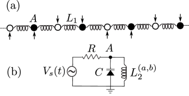
Figure 1: (a) Schematic circuit diagrams of the electrical lattice, where the blank points represents circuit cells of type $(a)$ and black points represent circuit cells of type $(b)$. Black arrows represent driving and its phase. (b) Each cell is connected to a periodic voltage source $V_{s}(t)$ via a resistor $R$, and grounded. Each point $A$ of an elemental circuit is connected via inductors $L_{1}$ to the corresponding points $A$ of neighboring cell. Voltages are monitored at point $A$.

Furthermore, the concrete parameter values of the system (comprised of inductors, resistors and capacitors) are $L_{1}=0.68$ mH, $L_{2}^{(a)}=102.7$ $\mu$H, $L_{2}^{(b)}=970$ $\mu$H, $R=10$ k$\Omega$ and a NTE 618 varactor, for which the capacitance at zero voltage is $C_{0}=770$ pF. The number of nodes of each type was $N^{(a)}=N^{(b)}$ = 16, equaling 16 unit cells for a total of 32 nodes. Experimentally, node voltages $V_{n}$ at points $A$ were measured at a rate of 2.5 MHz using a multichannel analog-to-digital converter.

It has been shown that the basic dynamics of this electrical network can be qualitatively described by a simple model where the introduction of an amplitude-dependent phenomenological resistor, $R_{l}$, in parallel to the cell capacitance, is enough to reproduce experimentally observed features quite well electric1 . Accordingly, the dimensionless equations of motion read

$$\frac{di_{n}}{d\tau}=\frac{L_{2}^{(a)}}{L_{1}}(v_{n+1}+v_{n-1}-2v_{n})-\frac{L_{2}^{(a)}}{L_{2}^{(n)}}v_{n}$$ (1)

$$\frac{dv_{n}}{d\tau}=\frac{1}{c(v_{n})}\left[i-i_{d}+\frac{\cos(\Omega\tau)}{\omega_{0}RC_{0}}-\frac{v_{n}}{\omega_{0}R_{e}C_{0}}\right],$$

where $L_{2}^{(n)}=L_{2}^{(a)}$ if site $(n)$ corresponds to nodes $(a)$, or $L_{2}^{(n)}=L_{2}^{(b)}$ if it corresponds to nodes $(b)$. The following dimensionless variables have been used: $\tau=\omega_{0}t$; $i_{n}=(I_{v}-I_{2})/(\omega_{0}C_{0}V_{d})$, where $I_{v}$ is the full current through the unit cell and $I_{2}$ is the current through the inductor $L_{2}^{(n)}$, both corresponding to cell $n$; $v_{n}=V_{n}/V_{d}$. Here, $V_{d}$ is the driver amplitude, and $V_{n}$ is the measured voltage at node $n$; $\Omega=\omega_{d}/\omega_{0}$, $\omega_{0}=1/\sqrt{L_{2}^{(a)}C_{0}}$; $i_{d}=I_{D}/(\omega_{0}C_{0}V_{d})$, where $I_{D}$ is the current through the varactor diode; $c=C(V)/C_{0}$, and $C(V)$ is the nonlinear capacitance of the diode. $R_{e}$ is the equivalent resistance so $1/R_{e}=1/R+1/R_{l}$.

III Results and Discussion

In the limit of no driving and for small-amplitude oscillations the linear modes possess frequencies grouped into two bands, as expected on the basis of the diatomic structure of the lattice. The top (optic-like) and bottom (acoustic-like) bands of the linear spectrum are found to lie within the intervals $[314-356]$ and $[645-666]$ kHz, respectively. A plot of the theoretical dispersion bands - obtained from linearizing Eq. (1) - is shown in Fig. 2, and the linear modes corresponding to top and bottom of the two bands are shown in Fig. 3. Using the spatial signature of the driving outlined before, we are able to experimentally excite and pump the linear mode of Fig. 3(c) and (b), and we proceed to explore the dynamics of such a mode for frequencies within the bandgap (i.e., in the regime of nonlinear, breather-like excitations flachrev ).

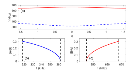
Figure 2: (a) Electrical line linear mode frequencies $f$ as function of the wavevector $q=n\pi/N$, where $n=-N/2\ldots N/2$ and $N=N^{(a)}+N^{(b)}$. A solid line is used to denote the top and a dashed to denote the bottom band. Figures (b) and (c) show the ratios between different linear mode amplitudes in the bands, where $A$ correspond to oscillation amplitudes of cells of type $(a)$ and $B$ to cells of type $(b)$.

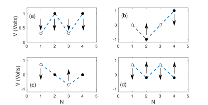
Figure 3: Different linear modes corresponding to the top and the bottom of the bands shown in Fig. 2 . (a) Uniform linear mode corresponding to the bottom of the lower band. (b) Linear mode corresponding to the top of the lower band, where the $L_{2}^{(b)}$ sub-lattice oscillates out-of-phase and the other sub-lattice is at rest. (c) Linear mode corresponding to the bottom of the upper band, where the $L_{2}^{(a)}$ sub-lattice oscillates out-of-phase, and the other sub-lattice is at rest. (d) Linear mode corresponding to the top of the upper band, where all neighboring cells oscillate out-of phase.

III.1 Dark gap breathers

The existence of bright ILMs below the lower linear dispersion band has been well established in such systems, driven either directly or with a subharmonic driver electric1 ; electric2 ; electric3 ; electric4 ; electric5 . In this work, we focus on the existence and properties of discrete breathers in the band-gap, where we have, remarkably, found both dark and bright breathers (with non-vanishing background), depending on the precise driver frequency within the gap.

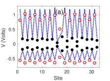
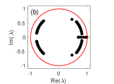
Figure 4: (a) Numerical (dotted line) and experimental (circles) dark breather profile (maximum and minimum amplitude) corresponding to $V_{d}=3.5$ Volts and $f=571$ kHz. Blank points represent circuit cells of type $(a)$ and black points represent circuit cells of type $(b)$. (b) Floquet multiplier numerical linearization spectrum confirming that, since all multipliers are inside the unit circle, the stability of the solution

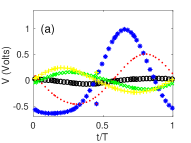
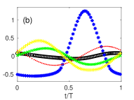
Figure 5: (a) Experimental and (b) numerical voltage oscillations of the dark breather corresponding to $V_{d}=3.5$ Volts and $f=571$ kHz: site 16 (black circles), first neighbors sites 15 (blue,diamond) and 17 (red dots), and second neighbors: sites 14 (green crosses) and 18 (yellow pluses).

Figure 4 shows the experimental result for driving at a frequency of 571 kHz, about 25% into the gap from above, and 74 kHz below the lower band-edge of the top band (the zone-boundary mode is at 645 kHz). The amplitude is $V_{d}=3.5$ Volts. The lattice profile of maximum and minimum node voltages in Fig. 4 clearly indicates the presence of a dark localized mode located around nodes 16 and 17. The term “dark” is used to describe a localized mode for which the amplitude of oscillation is large and constant in the lattice except at the ILM center and in its close vicinity (where it is near vanishing). Such structures, although theoretically proposed early on in guill , were only identified quite recently in a materials system (a granular crystal) in the work of granular2 . There, they were produced as a result of the destructive interference of waves emanating from the boundary, while here they are robustly created by the drive within the bandgap, as evidenced in the computational stability analysis of Fig. 4. Figure 5 shows the experimental time series at selected nodes. On one sublattice, node 17 (red dots) is suppressed relative to node 15 (blue diamonds), and on the other sublattice, node 16 (black, open circle) is suppressed relative to nodes 14 (green crosses) and 18 (yellow pluses). Experimentally (left panel), we see that the amplitude on the large-oscillation sublattice is reduced at the dark ILM center to about half the value in the wings. Numerically (left panel) the reduction is similarly (or even more) pronounced for these particular driving conditions.

In other experimental runs, the center of the dark ILM forms at different locations within the lattice, so this is not an impurity effect and as expected in a longer (nearly) homogeneous lattice the DB enjoys the discrete shift invariance of the diatomic chain. Nevertheless, we also observe that the the location can be predetermined (i.e., designed) by placing a temporary impurity at the chosen site before turning on the driver. The sign of the impurity necessary to seed a dark ILM is opposite to the one needed for bright ILMs. Numerically, we find stable one–peak dark breathers existing in the range of [569.5-600] kHz for a drive amplitude of $V_{d}=3.5$ Volts. It remains an important, albeit numerically rather demanding, question as to whether the dark breather can be found in computations throughout the system’s bandgap.

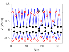
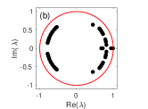
Figure 6: (a) Numerical (dotted line) and experimental (circles) two–peak dark breather profile (maximum and minimum amplitude) corresponding to $V_{d}=3.5$ Volts and $f=570$ kHz. Blank points represent circuit cells of type $(a)$ and black points represent circuit cells of type $(b)$. (b) Floquet multiplier numerical linearization spectrum confirming the stability of the solution since all multipliers are inside the unit circle.

Decreasing the driving frequency further into the bandgap, a pattern of multi-peak dark ILMs emerges, as shown in Fig. 7 . The number of dark ILMs in the lattice is very sensitive to the precise driver frequency at constant amplitude. In general, decreasing the driving frequency produces multi-peak structures and numerical solutions show overall good agreement with experimental results. However, numerics and experiments differ as to the precise localization centers, and in experiments they are found to be spaced somewhat more closely than in the numerical results. Nevertheless, the numerical results strongly suggest that such coherent structures should be dynamically robust, in line with the corresponding experimental observations. As also seen in previous studies, where the ILM is generated by a uniform driver, it can be sensitive to small lattice impurities which are, unfortunately, hard to completely eliminate in a manufactured lattice.

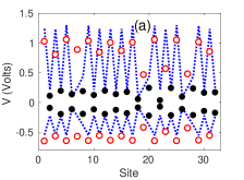
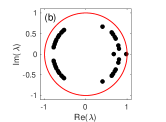
Figure 7: (a) Numerical (dotted line) and experimental (circles) three–peak dark breather profile (maximum and minimum amplitude) corresponding to $V_{d}=3.5$ Volts and $f=567$ kHz. Blank points represent circuit cells of type $(a)$ and black points represent circuit cells of type $(b)$. (b) Floquet multiplier numerical linearization spectrum confirming the stability of the solution since all multipliers are inside the unit circle.

III.2 Bright gap breathers

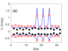
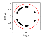
Figure 8: (a) Numerical (dotted line) and experimental (circles) three–peak bright breather profile (maximum and minimum amplitude) corresponding to $V_{d}=3.5$ Volts and $f=532$ kHz. Blank points represent circuit cells of type $(a)$ and black points represent circuit cells of type $(b)$. (b) Floquet multiplier numerical linearization spectrum confirming the stability of the solution.

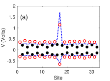
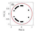
Figure 9: (a) Numerical (dotted line) and experimental (circles) one–peak bright breather profile (maximum and minimum amplitude) corresponding to $V_{d}=3.5$ Volts and $f=528$ kHz. Blank points represent circuit cells of type $(a)$ and black points represent circuit cells of type $(b)$. (b) Floquet multiplier numerical linearization spectrum confirming, similarly as above, the stability of the solution.

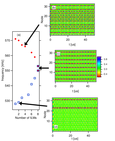
Figure 10: Summary of the progression from dark to bright multi-peak ILM structures. Panels (a) show the driver frequency as a function of the number of breathers, both dark (circles, red) and bright (squares, blue). At around 550 kHz, we observe an equal mixture of bright and dark breathers. (b) - (d) show the experimental data corresponding to select frequencies.

As we have seen, upon lowering the frequency, the DBs persist and apparently the number of their stable dips is increased within the chain. It is interesting that this is analogous to the phenomenology observed in the granular case, as discussed in granular2 . Nevertheless, as the frequency is further reduced, an unprecedented (to our knowledge) scenario develops. More specifically, the localized pattern inverts, i.e., an excited set of nodes appears above the background value. Thus, a train of bright (or perhaps anti-dark kivsharbook ) localized modes appears. If the frequency is further lowered within the gap, the peaks within this multi-peak pattern become more sparse until finally only a single such bright breather survives. Below this lower threshold, the driver cannot sustain any lattice modes at the given driving amplitude - linear or nonlinear - until we get into the vicinity of the bottom band. For an amplitude of 3.5V, the experimental threshold lies at 528 kHz, well above the upper edge of the bottom band.

Figures 8 and 9 depict these bright localized modes for two different drive frequencies, separated by 4 kHz. At the higher frequency, three ILMs survive, whereas at 528 kHz, we are left with a single bright breather. Let us briefly examine the spatial structure of this state. Its center always resides on the $L_{2}^{(a)}$ sublattice, namely on a cell with lower inductance, $L_{2}$. Further, these breathers are extremely sharp - the nearest neighbors on the $L_{2}^{(b)}$ sublattice register a slightly larger oscillation amplitude compared to the wings, but beyond that no increase beyond background can be discerned. The background oscillation is characterized by the $L_{2}^{(b)}$ sublattice almost at rest, undergoing only small oscillations, whereas the $L_{2}^{(a)}$ sublattice is oscillating out-of-phase. Thus, the ILM wings, or background, is consistent with the top (i.e., optic) zone-boundary mode pattern. These observations are in good agreement with numerical results. The precise width of any stability region is hard to match because there exist regions of different peak numbers and regions of different families with the same number of peaks that all overlap. While the close matching of the numerical and experimental pictures clearly validates the existence of these structures, a detailed bifurcation analysis associated with the frequency variations remains an intriguing topic for future study.

Figure 10(a) effectively summarizes the experimental picture and thus yields a first clue to the kind of bifurcation diagram mentioned above. In particular, it depicts the transition from dark to bright breathers as the frequency is lowered starting closer to the bottom of the top mode and moving progressively deeper into the bandgap. At the highest frequency considered within the gap, the zone-boundary plane-wave mode is excited at high amplitude. As the frequency is somewhat lowered, first a single dark breather, and then multi-peak dark DBs, are generated. Then, as the frequency is further lowered into the bandgap, eventually a striped nonlinear pattern is seen (Fig. 10(c)), which could also be characterized as a (roughly) equal mixture of bright and dark breathers. Below that frequency, we observe bright breathers, whose numbers in the lattice decrease as the drive frequency is further lowered. It is worth noting that the bright breathers, when multiple of them arise, are found to always be in phase.

The supporting panels, Fig. 10(b)-(d), depict the experimental data in time and space at select drive frequencies. This is one of the especially appealing aspects of this system, namely the ability for distributed characterization/visualization of the dynamics (in addition to the distributed driving capabilities for this system). Note that the pattern characterizing equal numbers of bright and dark ILMs is qualitatively different from the nonlinear zone-boundary mode. In fact, its spatial periodicity is doubled, and one could describe the resulting pattern as a dynamically induced superlattice. We also note that while the dark breathers are sharply localized in this system (as are the bright ones), they do encompass several lattice nodes. Finally, the dark breathers can be shepherded spatially via temporarily induced impurities at neighboring sites. This tunability can be important for the controllable transfer of energy within such a system.

III.3 Near the bottom band

The vicinity of the bottom band also features bright and dark ILMs. Figure 11 depicts the situation at a driver frequency of 280 kHz, just below the bottom of the band. One dark breather is clearly visible at site n=13 in the experimental data. Simulations also find this dark breather, although the background amplitude is slightly higher than in the experiment under identical driving conditions. Floquet analysis again shows that this mode is dynamically stable; see Fig. 11(b).

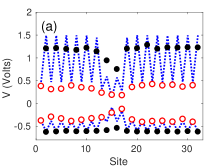
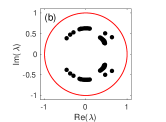
Figure 11: (a) Numerical (dotted line) and experimental (circles) dark breather profile (maximum and minimum amplitude) corresponding to $V_{d}=3.5$ Volts and $f=280$ kHz. Blank points represent circuit cells of type $(a)$ and black points represent circuit cells of type $(b)$. (b) Floquet multiplier numerical linearization spectrum confirming the stability of the solution.

If the driving frequency is lowered by a mere 10 kHz to 270 kHz, bright ILMs are generated. These bright ILMs just below the bottom band are different from the bright ILMs of the top band in that their localization centers are on the opposite sublattice, namely the sublattice of $L_{2}^{(b)}$ sites characterized by the larger inductance value. The situation is succinctly depicted in Fig. 12 where so-called frequency shift key modulation (FSK) is employed to switch the driver frequency abruptly from one value to another. Here a shift from 271 kHz to 543 kHz was initiated in the experiment at a time of 2000 $\mu$s. The first frequency is consistent with two bright breathers with the associated (lower) frequency, whereas the second generates two bright breathers with the corresponding (higher) frequency in a different location. We see that the breathers are initially located on even sites, but after 2000 $\mu$s quickly settle on odd sites.

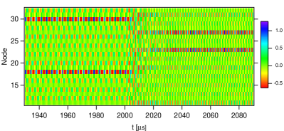
Figure 12: Experimental FSK modulation that switches abruptly between two distinct values of the driving frequency while keeping the amplitude fixed at 3.5 V. Initially, for $f=$271 kHz, two breathers are seen, but then when the frequency switches to 543 kHz, two distinct ILMs at a different location with the latter frequency (centered on odd sites) develop.

IV Conclusions & Future Work

In the present work, we have examined the setting of electrical lattices in the form of a controllable/tunable diatomic-like system. Building on the modeling successfully used earlier for the monatomic case, we have considered both the linear and especially the nonlinear properties of this system, examining them in parallel both at the experimental and numerical level. We have found these lattices to be very useful playgrounds for the exploration of dark breather and multi-breather structures. Such states have spontaneously emerged in the experiments at different frequencies within the bandgap near the top band. However, as one further lowers the frequency, a bright nonlinear structure (on top of a background) emerged, involving initially multiple peaks, which then become progressively fewer (as the frequency was further lowered), before eventually disappearing altogether well above the cutoff frequency of the bottom band.

While the structures reported here, we feel, are intriguing, they also pose numerous open questions for future consideration. Many of these can be addressed by a systematic analysis of the bifurcations of single and multiple dark and bright breathers in the bandgap. Such an analysis, while computationally demanding, would offer a more systematic roadmap for future experiments. There we could explore what happens in the immediate vicinity of the (upper edge of the) bottom branch, as well as the (lower edge of the) top branch. Extensions of these fairly controllable structures would also be worthwhile to consider in higher dimensional systems. Some of these questions are currently under consideration and will be reported in future publications.

- (1) A.J. Sievers, S. Takeno, Phys. Rev. Lett. 61, 970 (1988).
- (2) S. Takeno, K. Kisoda, A.J. Sievers, Prog. Theor. Phys. Suppl. 94, 242 (1988).
- (3) R.S. MacKay, S. Aubry, Nonlinearity 7, 1623 (1994).
- (4) E. Trías, J.J. Mazo, T.P. Orlando, Phys. Rev. Lett. 84, 741 (2000).
- (5) P. Binder, D. Abraimov, A.V. Ustinov, S. Flach, Y. Zolotaryuk, Phys. Rev. Lett. 84, 745 (2000).
- (6) J. Cuevas, L.Q. English, P.G. Kevrekidis, M. Anderson, Phys. Rev. Lett. 102, 224101 (2009).
- (7) F. Palmero, J. Han, L.Q. English, T.J. Alexander, P.G. Kevrekidis, Phys. Lett. A 380, 401 (2016).
- (8) F.M. Russell, Y. Zolotaryuk, J.C. Eilbeck, T. Dauxois, Phys. Rev. B 55, 6304 (1997).
- (9) M. Sato, B.E. Hubbard, A.J. Sievers. Rev. Mod. Phys. 78, 137 (2006).
- (10) F. Palmero, L.Q. English, J. Cuevas, R. Carretero-González, P.G. Kevrekidis, Phys. Rev. E 84, 026605 (2011).
- (11) L.Q. English, F. Palmero, J.F. Stormes, J. Cuevas, R. Carretero-González, P.G. Kevrekidis, Phys. Rev. E 88, 022912 (2013).
- (12) N. Boechler, G. Theocharis, S. Job, P. G. Kevrekidis, Mason A. Porter, and C. Daraio Phys. Rev. Lett. 104, 244302 (2010).
- (13) C. Chong, F. Li, J. Yang, M.O. Williams, I.G. Kevrekidis, P.G. Kevrekidis, C. Daraio, Phys. Rev. E 89, 032924 (2014).
- (14) B.I. Swanson, J.A. Brozik, S.P. Love, G.F. Strouse, A.P. Shreve, A.R. Bishop, W.-Z. Wang, M.I. Salkola, Phys. Rev. Lett. 82, 3288 (1999).
- (15) M. Sato, A.J. Sievers, Nature 432, 486 (2004).
- (16) M. Peyrard, Nonlinearity 17, R1 (2004).
- (17) M.E. Manley, M. Yethiraj, H. Sinn, H.M. Volz, A. Alatas, J.C. Lashley, W.L. Hults, G.H. Lander, J. L. Smith, Phys. Rev. Lett. 96, 125501 (2006).
- (18) M.E. Manley, A.J. Sievers, J.W. Lynn, S.A. Kiselev, N.I. Agladze, Y. Chen, A. Llobet, A. Alatas, Phys. Rev. B 79, 134304 (2009).
- (19) S. Flach and A. V. Gorbach, Phys. Rep. 467, 1 (2008).
- (20) M. Remoissenet, Waves called solitons, Springer-Verlag (New York, 1999).
- (21) L.Q. English, F. Palmero, P. Candiani, J. Cuevas, R. Carretero-Gonzalez, P. G. Kevrekidis, and A.J. Sievers, Phys. Rev. Lett. 108, 084101 (2012).
- (22) M. Sato, S. Yasui, M. Kimura, T. Hikihara, A. J. Sievers, EPL 80, 30002 (2007).
- (23) L.Q. English, R.B. Thakur, R. Stearrett, Phys. Rev. E 77, 066601 (2008).
- (24) L. Q. English, F.Palmero, P. Candiani, J. Cuevas, R. Carretero-González, P. G. Kevrekidis and A. J. Sievers, Phys. Rev. Lett., 108, 084101 (2012).
- (25) Xuan-Lin Chen, Saidou Abdoulkary, P. G. Kevrekidis, and L. Q. English, Phys. Rev. E 98, 052201 (2018).
- (26) T. Kofane, B. Michaux, M. Remoissenet, J. Phys. C: Solid State Phys. 21, 1395 (1988).
- (27) A. Álvarez, J.F.R. Archilla, J. Cuevas, and F.R. Romero, New J. Phys. 4, 1 (2002).
- (28) B. Sánchez-Rey, G. James, J. Cuevas, and J. F. R. Archilla Phys. Rev. B 70, 014301 (2004).
- (29) C. Chong, P. G. Kevrekidis, G. Theocharis, and Chiara Daraio Phys. Rev. E 87, 042202 (2013).
- (30) Yu.S. Kivshar and G.P. Agrawal, Optical solitons: from fibers to photonic crystals, Academic Press (San Diego, 2003).