Prediction and forecasting models based on patient’s history and biomarkers with application to Scleroderma disease

Abstract

This paper aims at predicting lung function values based on patients historical lung function values and serum biomarkers in Scleroderma patients. The progression of disease is measured by three lung function indexes (FVC, TLC, DLCO). Values of four biomarkers (TIMP1, P3NP, HA, NT-proBNP) are available. The data are sparse (6 months intervals) and irregular (many visits are missed). We consider two modeling approaches to achieve our goal, namely, the mixed effects model which is the standard approach in epidemiological studies and the functional principal component analysis model which is typically used for dense temporal datasets. We find that functional data methodology was able to recover the trajectories of three lung function indexes and to predict the future values very well.

Keywords: functional principal component analysis, mixed effects model, prediction, Scleroderma, sparse and irregular functional data.

1 Introduction

With the introduction of the Electronic Health Records (EHR), it is now possible to use retrospective information on outcomes, biomakers and classical risk factors to build a prediction model for a specific outcome. These models can be used for decision making with regards to planning of hospital visits, expensive measurements and treatment. Especially for diseases with heterogeneous trajectories, i.e. where the progress and type of the disease differ across patients, patient specific prediction is relevant. Unfortunately, building models from EHR data is often complex. The visits of patients are typically irregular and sparse and the number of patients with regular observations might be small. The heterogeneity in disease and underlying risks needs to be taken into account. Finally the data are typically noisy.

In epidemiology linear mixed models are often used to model the relationship between biomarkers and a repeatedly measured outcome. Here correlation between measurements for the same person is modeled via random effects. For mixed effects model theory see Verbeke and Molenberghs (2009), Hedeker and Gibbons (2006), Wu and Zhang (2006), Wu and Tian (2018) and the references therein. Forecasting of future disease trajectories based on the current values of the risk factors, covariates and outcomes might be performed with these models, see Skrondal and Rabe-Hesketh (2009).

Alternative approaches are in the framework of functional data analysis. The advantages of these latter methods are that they are very flexible with regard to the functional model for the outcome over time and they can deal with irregular and sparse data, see e.g. Beran and Liu (2014, 2016), Peng and Paul (2009), Yao et al. (2005), James (2010), James et al. (2000). For general methods and theory on functional data analysis, one may refer to the monographs such as Ramsay and Silverman (2005), Horvath and Kokoszka (2012), Kokoszka and Reimherr (2017) and the references therein. In the FDA framework estimation of future disease trajectories is straightforward, in contrast to predictions based on a mixed model, which requires integration over the posterior multivariate distribution of the random effects. On the other hand, a mixed model provides a straightforward prediction of the outcome by just filling in the covariate values and zeros for the random effects. This paper is motivated by an ongoing study on predicting the disease trajectory of Scleroderma patients. Here we discuss methods for prediction of expensive measurements based on historical and biomarker data. We will consider linear mixed models and functional data analysis for this purpose.

We will build prediction models for Scleroderma disease. Scleroderma disease is a rare, clinically heterogeneous multisystem disorder which might affect the patients’ physical and psychological functioning and impairs their ability to participate in work and social activities (see Jaeger et al. 2017, Gabrielli et al. 2009, and Muangchan et al. 2013). The disease is heterogeneous since only 30% of the patients progress to a severe disease status. Further the patients can progress to various outcomes. Currently, the most common outcomes of disease progression include modified rodnan skin score (mRSS) and three lung functions (FVC, TLC, DLCO) which are age and gender specific predicted percentages. In this paper, we will not consider mRSS since it is quite noisy and depends on the observer (see Khanna et al. 2017 and Clements et al. 1993). Since the lung functions are expensive measurements, good predictions of these functions based on historical or biomarker data will be valuable. Further, we have data on four candidate biomarkers, namely TIMP1, P3NP, HA, and NT-proBNP. In the rest of the paper, we denote TIMP1 by TIMP and NT-proBNP by NT.

Data for this study come from outpatient EHRs of patients attending Scleroderma clinics every six months. Scleroderma patients visit the hospital every six months. In our dataset the number of patients with regular visits is very limited. On the other hand we have a few patients with several measurements over a longer time period. To assess prediction accuracy based on current values of the biomarkers we will use linear mixed models for a subset of patients with at least two observations at 0, 6, 12 months. Since the outcomes change continually over time, they are functional data. We propose therefore to use a functional principal component analysis (FPCA) method to predict the future values of outcomes. Here we use the subset of patients who have at least two observations in the first 60 months. Restricted maximum likelihood framework is used to estimate the eigenelements of underlying covariance operator (see Peng and Paul 2009) and the scores are estimated by the principal components analysis through conditional expectation (PACE) method (see Yao et al. 2005). Then the trajectories are recovered by using the truncated Karhunen-Loève decomposition based on the estimated eigenelements and scores.

In section 2 we describe the dataset in more detail. In Section 3 we will introduce the methods. Section 4 presents the results. Finally section 5 is a conclusion and future research lines are provided.

2 Dataset

In total, 255 Scleroderma patients with information from hospital visits from 1995 to 2015 have been retrospectively recruited to our study, the majority of the observations are from after 2010). Data were collected according to ethically approved protocol for observational study HRA number 15/NE/0211. Typically, the Scleroderma patients visit hospital every six months. However, many patients missed their appointments or data were not recorded. Therefore, our dataset has only 573 observations. We have three lung function indexes FVC, TLC, DLCO with values larger than 0 and small values for severe disease. Four biomarkers are measured, namely TIMP, P3NP, HA and NT. After removing the observations with missing values, our dataset comprises 421 measurements from 208 patients. Further data cleaning results in 316 measurements from 117 patients see Figure 1 for details.

First for mixed effects models, we select the patients who have at least two observations at 0, 6, 12 months and the number of patients is 73. Second for the functional data analysis model, we use all the 117 patients for modelling. For forecasting, we need patients at least three observations in the first 60 months and the number of patients is 60.

The profiles of these patients with regard to the biomarkers and outcomes are depicted in Figure 2. Figure 2 also shows that the observations are sparse, irregular and unbalanced, with more observations in the first two years and less in the last two years. From these patients, only 60 patients (with 202 measurements) have data for at least three visits. For time 0, i.e. the first visit time, the mean and covariance of biomarker and outcomes are shown in Table 1. The correlations between FVC, TLC and DLCO are quite large, with the largest value of 0.80 for the correlation between FVC and TLC. The correlations between the biomarkers are smaller and range from 0.15 to 0.44.

	TIMP	P3NP	HA	NT	FVC	TLC	DLCO
mean
	234	7	49	130	102	93	65
variance
	3188	11	2098	14875	540	329	267
correlation
TIMP	1.00	0.35	0.30	0.21	-0.21	-0.28	-0.19
P3NP		1.00	0.44	0.15	-0.32	-0.35	-0.36
HA			1.00	0.15	0.05	-0.08	-0.04
NT				1.00	-0.08	-0.21	-0.21
FVC					1.00	0.80	0.47
TLC						1.00	0.51
DLCO							1.00

Table 1: At time 0 (112 observations), mean and variance of biomarkers and outcomes, correlations between biomarkers and outcomes.

Figure 1: Patient chart flow.

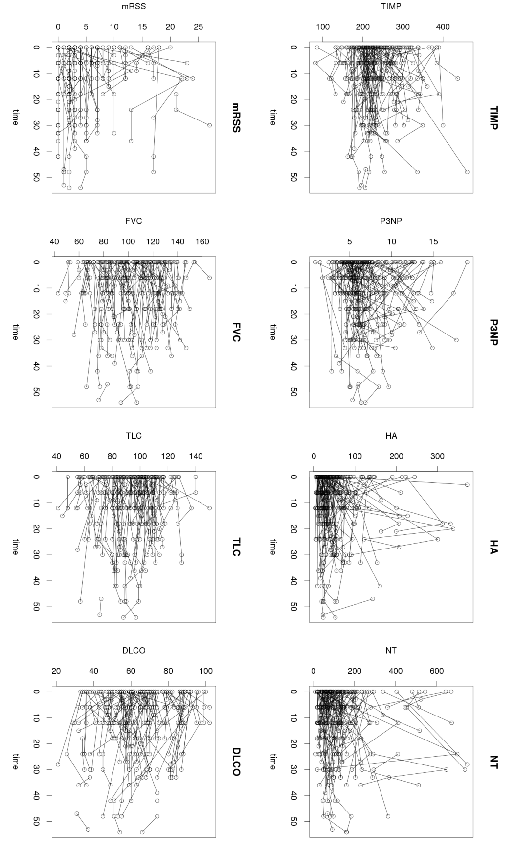
Figure 2: Clean data.

3 Methods

Our aim is to predict and forecast the lung functions by using either biomarkers or past lung function values. The classical way to analyse sparse longitudinal data is the linear mixed effects model. The grid of visits should be regular although missing outcomes for some visits are allowed. Alternatively sparse and irregular longitudinal data are functional data, and forecasting based on historical outcomes can be performed by using functional principal component analyses. For our dataset we will consider both methods.

3.1 Linear mixed effects models

To model the relationship between biomarkers and lung function indexes, linear mixed effects models are fitted to the data from patients with observations at time 0 ($n=73$) and at least one observation at 6 months ($n=42$) or at 12 months ($n=44$).

For individual $i$ ($i=1,...,73$) and measurement $j$ ($j=1,...,N_{i}$ with $N_{i}\in\{2,\ 3\}$ the number of observations for individual $i$), let $y_{ij}$ be the observation at time $t_{ij}$, $x_{ij}$ be the logarithm of the value of the biomarker for individual $i$ at time $t_{ij}$. Then the following linear mixed effects model is considered

$$y_{ij}=\beta_{0}+\beta_{1}t_{ij}+\beta_{2}x_{ij}+\gamma_{0i}+\gamma_{1i}t_{ij}+e_{ij}$$ (1)

where $t_{ij}=0,6$ or 12 months, $\beta_{0j}+\beta_{1}t_{ij}$ is the time specific intercept and $\beta_{2j}$ represents the effect of the biomarker at time point $t_{ij}$. The the person specific random intercept $\gamma_{0i}$ and slope $\gamma_{1i}$ model follow the following distribution

$$(\gamma_{0i},\gamma_{1i})^{T}\sim N(0,\Sigma)$$

with

$$\Sigma=\left({\begin{array}[]{cc}\sigma^{2}_{0}&\sigma_{01}\\ \sigma_{01}&\sigma^{2}_{1}\\ \end{array}}\right).$$

Finally the term $e_{ij}$ is the random residual. Note that since it is expected that heterogeneity across the patients with regard to disease progress exist we included a random intercept and slope.

Based on the linear mixed model, a prediction for a new lung function value can be computed based on current biomarkers by plugging in the mean of the random effects (i.e. 0) in (1) (see Skrondal and Rabe-Hesketh 2009). To evaluate the prediction accuracy of this model, the cross validated mean squared error (MSE) is computed. To this end we base the prediction of the vector of outcomes $y_{i}$ on the vector of biomarkers $x_{i}$ and a model fitted on the data set obtained by leaving out the data of indivivual $i$. Specifically

$$\hat{y}_{ij}=\hat{\beta}^{(-i)}_{0}+\hat{\beta}^{(-i)}_{1}x_{ij}+\hat{\beta}^{(-i)}_{2}t_{ij}$$

where $\hat{\beta}^{(-i)}_{0},\hat{\beta}^{(-i)}_{1},\hat{\beta}^{(-i)}_{2}$ are the corresponding estimates of $\beta_{0},\beta_{1},\beta_{2}$ of model (1) on the data set obtained by leaving out the observations of individual $i$. Now the leave one out cross validated average MSE is defined as:

$$MSE=\frac{1}{\sum_{i=1}^{n}N_{i}}\sum_{i=1}^{n}\sum_{j=1}^{N_{i}}(y_{ij}-\hat{y}_{ij})^{2}.$$

In principle linear mixed models can also be used to forecast a new measurement in an existing cluster. However since in our dataset we have only a few patients ($n=13$) who have three observations at 0, 6, 12 months, the performance of these predictions cannot be evaluated. An alternative is functional principal component analysis.

3.2 Functional principal component analysis

Let $X_{i}(t)$ be the trajectory of the $i$th patient, where $i\in\{1,...,n\},\ t\in[0,1]$. Here the time scale is transformed from 0 to 60 months to $[0,1]$. We assume $X_{i}(t)$ are independent realizations of a squared integrable random function $X(t)$ on $[0,1]$, i.e. $X(t)\in L^{2}[0,1]$. We denote $\mu(t)=E[X(t)]$ the mean function of $X(t)$ and $C(s,t)=E[(X(s)-\mu(s))(X(t)-\mu(t))]$ the covariance function of $X(t)$, then by Mercer’s theorem

$$C(s,t)=\sum_{l=1}^{\infty}\lambda_{l}\phi_{l}(s)\phi_{l}(t)$$

where $\lambda_{1}\geq\lambda_{2}\geq...\geq 0$ with $\sum\lambda_{l}<\infty$ are the eigenvalues of $C$. $\phi_{l}(t)$ is the $l$th eigenfunction corresponding to $\lambda_{l}$ and $\{\phi_{l}\}$ forms a complete orthonormal basis for $L^{2}[0,1]$. Then $X_{i}(t)$ has the following Karhunen-Loève decomposition

$$X_{i}(t)=\mu(t)+\sum_{l=1}^{\infty}\xi_{il}\phi_{l}(t)$$

where $\xi_{il}=\int(X_{i}(t)-\mu(t))\phi_{l}(t)dt$ is the associated functional principal score with $var(\xi_{il})=\lambda_{l}$ and $\phi_{l}$ is also called the $l$th functional principal component. In practice, $X_{i}(t)$ is usually well approximated by the first $L$ leading functional principal components and scores

$$\tilde{X}_{i}(t)=\mu(t)+\sum_{l=1}^{L}\xi_{il}\phi_{l}(t)$$

For patient $i$ the trajectory $X_{i}(t)$ is observed at a sparse grid $t_{i1},...t_{iN_{i}}$. For example, $X_{i}(t_{i1}),..,X_{i}(t_{i_{N_{i}}})$ are the observed discrete DLCO values for patient $i$ at time $t_{i1}...,t_{i_{N_{i}}}$ (after rescaling). The number and spacing of the observed time points vary per patient, i.e. for $i\neq j$, $N_{i}$ and $N_{j}$ might be different and $t_{i2}-t_{i1}$ might be different from $t_{j2}-t_{j1}$.

In order to recover the individual-specific curves $X_{i}(t)$, one has to estimate the mean function $\mu(t)$, FPC scores $\xi_{il}$, FPCs $\phi(t)$, and determine the number of FPCs to be included $L$. The mean function $\mu(t)$ is estimated by a local linear smoother and it is subtracted from the observations before estimating the other model parameters.

Since the eigenfunctions corresponding to the largest several eigenvalues can be well approximated by using less complex basis, cubic B-spline basis with equally spaced knots is used to expand $\phi_{l}$. Under the Gaussianity of the process, i.e. $\xi_{il}\overset{iid}{\sim}N(0,\lambda_{l})$ and the errors $\epsilon$ are normal, the coefficients of expansion of $\phi_{l}$, eigenvalues $\lambda_{l}$ and other nuisance parameters can be estimated through the restricted maximum likelihood procedure proposed by Peng and Paul (2009). The number of nonzero eigenvalues and the number of basis for representing the eigenfunctions are selected by leave-one-curve-out cross-validation criteria.

Finally, for each patient, we need to estimate the FPC scores. The traditional way to estimate the FPC scores $\xi_{il}=\langle X_{i}-\mu,\phi_{l}\rangle$ is through numerical integration if the sampling is dense, see e.g. Beran and Liu (2016). However, for sparse functional data, numerical integration estimator will not be a reasonable estimate of $\xi_{il}$. Under the Gaussian assumption on the process, the estimation of FPC scores can be obtained based on conditional expectation proposed by Mardia et al. (1979) or Yao et al. (2005).

Once obtaining $\hat{\mu}(t)$, $\hat{\phi}_{l}(t)$, $\hat{\xi}_{il}$ and the number of nonzero eigenvalues $L$, the trajectory of the $i$th patient can be estimated by

$$\hat{X}_{i}(t)=\hat{\mu}(t)+\sum_{l=1}^{L}\hat{\xi}_{il}\hat{\phi}_{l}(t).$$ (2)

After selecting the number of nonzero eigenvalues $L$ and estimating the mean curve $\hat{\mu}(t)$, the corresponding FPC $\hat{\phi}_{l}(t)$ and the FPC score $\hat{\xi}_{il}$ from all available data, we can estimate missing values and predict future values of individual $i$ using the recovered trajectory (2)

$$\hat{X}_{i}(t)=\hat{\mu}(t)+\sum_{l=1}^{L}\hat{\xi}_{il}\hat{\phi}_{l}(t)$$

where time $t$ can be any past or future time points.

To evaluate the accuracy in forecasting lung function values, the cross validated mean square error can be computed. For patients who have more than two observations ($n=60$), we predict the last visit value by using all previous outcomes of this patient and by borrowing the information of all the other patients ($n=117$) using the above FPCA method. Thus to predict the last value for individual $i$, the training set on which the model is based, includes the information of all the patients except for the value of the last visit of patient $i$. The forecast is given by

$$\hat{X}_{i}^{(-last)}(t)=\hat{\mu}^{(-last)}(t)+\sum_{l=1}^{L^{(-last)}}\hat{\xi}^{(-last)}_{il}\hat{\phi}^{(-last)}_{l}(t)$$

where $\hat{\mu}^{(-last)}(t)$ is a local linear estimator of $\mu(t)$ with the last value of individual $i$ being excluded, $\hat{\phi}^{(-last)}_{l}(t)$ is the estimator of $\phi_{l}(t)$ with the last value of individual $i$ being excluded, $\hat{\xi}^{(-last)}_{il}$ is the estimator of $\phi_{l}(t)$ with the last value of individual $i$ being excluded, $L^{(-last)}$ is the number of nonzero eigenvalues selected by CV with the last value of individual $i$ being excluded. Therefore, the estimation of the last value of individual $i$ by using its own historical information and all the information of others is given by

$$\hat{X}_{i}^{(-last)}(t_{i,last})=\hat{\mu}^{(-last)}(t_{i,last})+\sum_{l=1}^{L^{(-last)}}\hat{\xi}^{(-last)}_{il}\hat{\phi}^{(-last)}_{l}(t_{i,last})$$

where $t_{i,last}$ is the last visiting time for individual $i$.

To assess the accuracy of the forcasts the mean squared errors are computed, i.e.

$$MSE=\frac{1}{n}\sum_{i=1}^{n}(x_{i}-\hat{x}_{i})^{2}.$$

for observations are $x_{1},...,x_{n}$ and corresponding prediction values are $\hat{x}_{1},...,\hat{x}_{n}$.

Finally the coefficient of determination $R^{2}$ which assesses the importance of the improvement in fit from the simpler model is computed:

$$R^{2}=1-\frac{MSE_{1}}{MSE_{0}},$$

where $MSE_{1}$ and $MSE_{0}$ are the MSE for the model based on the historical values and the null model, respectively.

Finally we assess whether the biomarkers have an effect on the forcast. We regress the residuals of the predicted values of the three outcomes (FVC, TLC, DLCO), i.e. $r_{i,t_{i,last}}=X_{i}(t_{i,last})-\hat{X}_{i}^{(-last)}(t_{i.last})$, on the observed values of the biomarker $z_{i,t_{i,last}}$ at last time points for the patients who have at least three observations ($n=60$). Specifically, we consider the simple linear regression

$$r_{i,t_{i,last}}=\alpha+\beta z_{i,t_{i,last}}+\epsilon_{i}$$

and denote the estimated intercept and slope as $\hat{\alpha}$ and $\hat{\beta}$ respectively. Then the residuals are estimated as $\hat{r}_{i,t_{i,last}}=\hat{\alpha}+\hat{\beta}z_{i,t_{i,last}}$. We then compute our updated predicted value as

$$\hat{X}_{i}(t_{i.last})=\hat{X}_{i}^{(-last)}(t_{i.last})+\hat{r}_{i,t_{i,last}}$$

Notice that for NT, the logarithm transformation is used.

4 Results

4.1 Linear mixed effects models

For each combination of lung function index (FVC, TLC, DLCO) and biomarker (TIMP, P3NP, HA, NT), linear mixed model (1) is fitted. Table 2 shows the $p$-values of the chi-square tests which compare the model with the biomarker to the null model without a biomarker. It appears that there is not much evidence for an association between the biomarkers and the lung function indexes. Only the effect of P3NP on DLCO is statistically significant at the 5% level.

	TIMP	P3NP	HA	NT
FVC	0.25	0.21	0.68	0.99
TLC	0.87	0.61	0.38	0.37
DLCO	0.13	0.02	0.85	0.52

Table 2: The $p$-values for the effects of the biomarkers on the outcomes.

For each lung function biomarker combination, the leave one out cross validated average MSE of the prediction based on the mixed effects model is given in Table 3. Here, also the leave one out cross validated average MSE of the prediction is given based on a mixed effects model without the biomarker (null model). It appears that the mixed effects models including one of the biomarkers only slightly improve the prediction compared to the null model. The largest improvement is 5.3 % for the combination of P3NP on DLCO.

	TIMP	P3NP	HA	NT	null
FVC	644	646	654	650	649
TLC	405	400	405	401	401
DLCO	306	300	320	318	317

Table 3: The cross validated MSE’s for predictions based on various model. Null is the model without a biomarker, i.e. only time is included in the mixed effects model

4.2 Functional principal component analysis

The estimated mean functions of the outcomes (FVC, TLC, DLCO) decrease during the whole period of five years (see Figure 3). Note that we rescaled the 60 months into a [0, 1] interval. All the biomarkers increase in the first two to three years. During the last two to three years, the biomarkers P3NP, HA and NT have a decreasing trend. At the end of the interval the estimate of the curves for the biomarkers appears to be uncertainty, which is probably caused by the lack of sampling points at the end of the interval (see Figure 2).

The mean function for mRSS has a decreasing trend. Note, however, that the measurement error is around 5 points, hence the slight decrease is not medical relevant and we may assume that the mean function is constant over time.

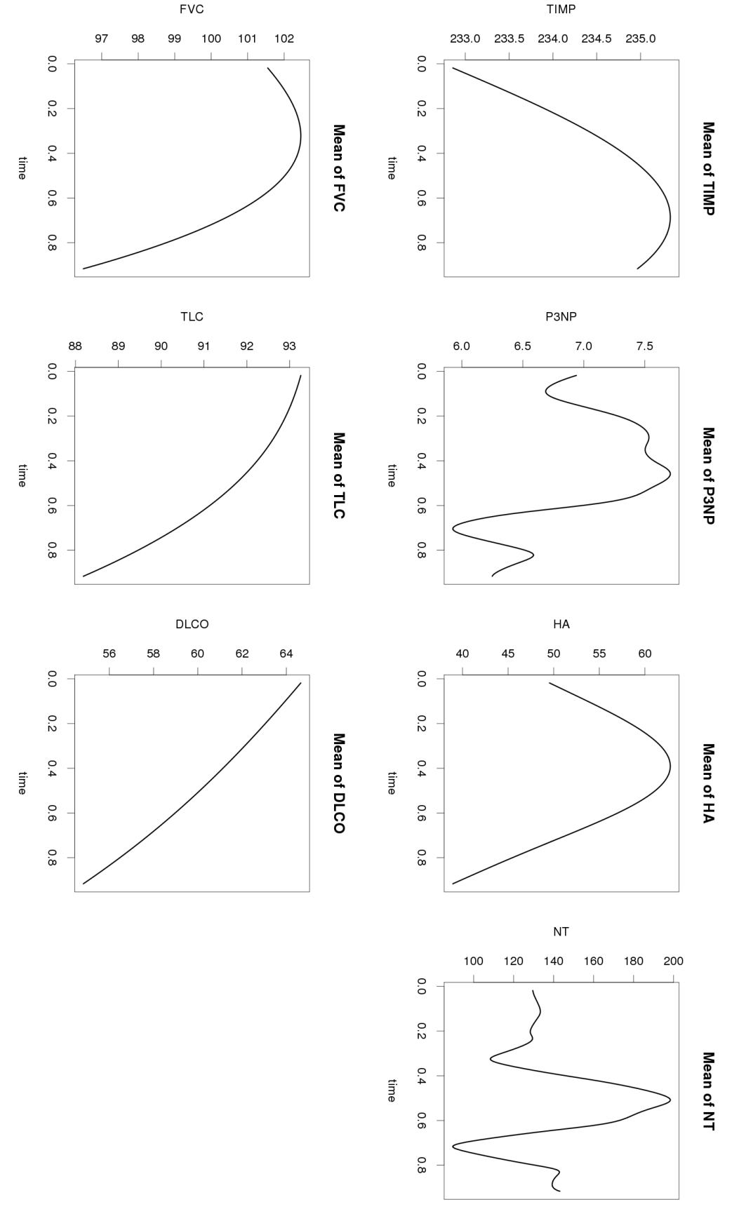
Figure 3: Mean.

We used two or three principal components to approximate the individual curves. Figure 4 displays the curves for the first 10 patients for TIMP, P3NP, HA, NT, FVC, TLC, and DLCO (from bottom to top). Overall, the trajectories for each patient captures the behavior of the observations. For the batches of blue lines, the recovered cures fluctuate due to the shape of the mean functions (see Figure 3).

Figure 4: Trajectory.

In order to quantify the prediction performance of our FPCA model, the predicted values of the last visit are computed. We only predicted the last values of the patients who have at least three measurements ($n=60$ patients). Figure 5 shows the prediction results. Here the blue points are the predicted values, and the black points are the observed values. The length of the red bars are the prediction errors. We observe that in general the predictions are good, however for patients who had a long period between the last and the previous visit and for time points in the second half of the time interval, the prediction error appears to be larger. This is probably due to lack of information to predict this value.

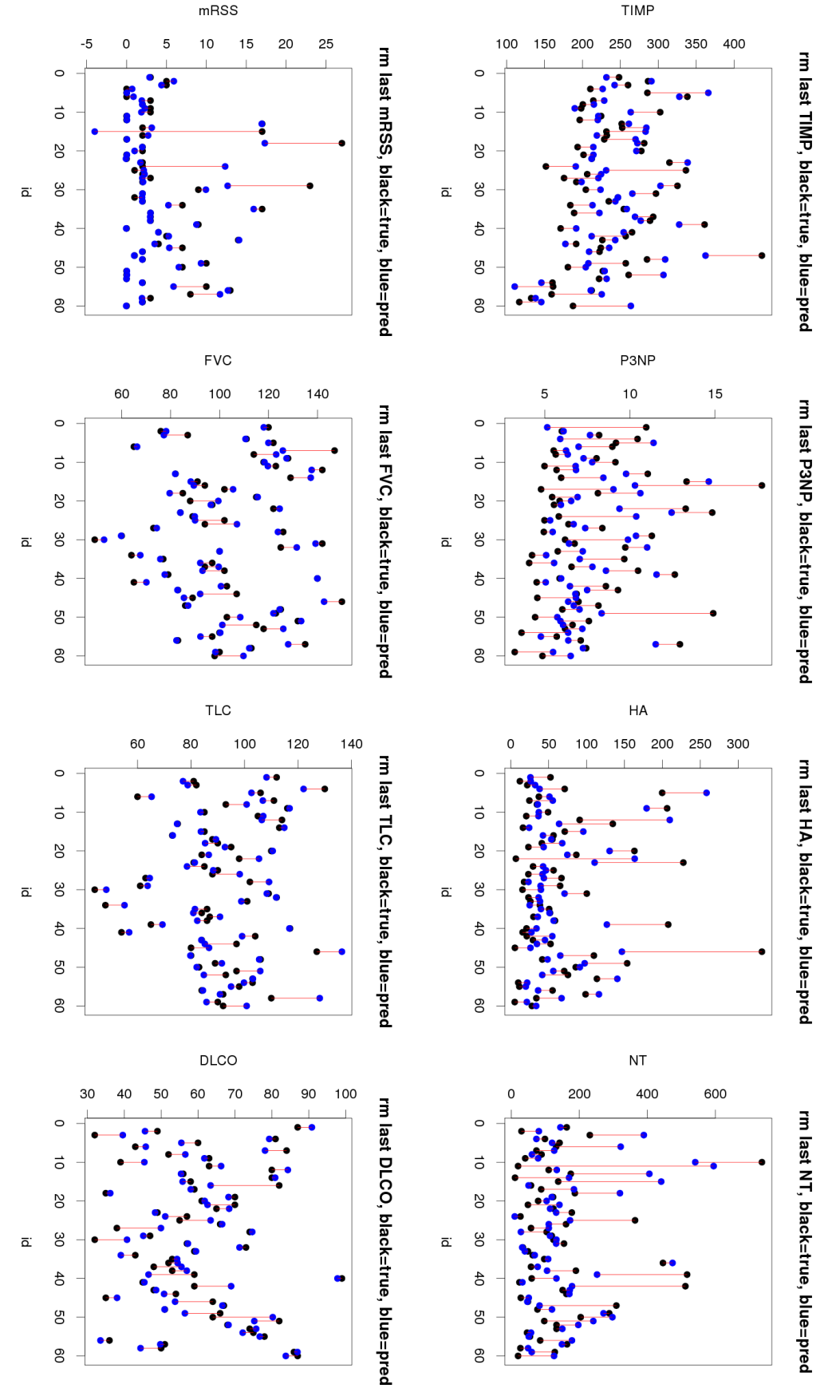
Figure 5: Prediction.

The cross validated MSE’s for the prediction are shown in Table 4. The cross validated MSE for the null model, i.e. prediction of the last value by the average of the 60 patients is also provided. Compared to the null model, our model has a much smaller cross validated MSE. In addition the improvement in prediction using historical data is better (90% reduction in MSE) than the improvement in prediction by using the biomarkers in the mixed-effects model (1% reduction in MSE) (Table 3). Table 4 also shows the MSE for the subgroup of patients who have a time interval of less than six months between the last and previous visit (near) (41 out of 60 patients) and the remaining patients (far) (19 out of 60 patients). We also considered the cross validated MSE in the subgroup of patients who have their last visit in the first 24 months (early) (36 out of 60 patients) and the remaining patients (late) (24 out of 60 patients). The MSE for “near” and “early” groups are smaller for most outcomes than for “far” and “late” group, because for these groups more information (more visits and more patients) is available. For TLC, there is not much difference between “early” and “late” groups. However, there is a difference between “near” and “far” groups, where the ”far” group performs better. The reason is that for the “near” group the variation between the last two observations in each individual is quite large. Our model has difficulties in capturing this since we used the B-spline basis. Finally the coefficient of determinations are given in Table 4. Here the smallest coefficient is 0.87 (DLCO).

	MSE						R2
	null	full	near	far	early	late	full
# patients	60	60	41	19	36	25	60
FVC	538	39	32	53	23	62	0.93
TLC	327	27	31	20	28	27	0.92
DLCO	244	32	22	55	21	49	0.87

Table 4: Results of forecasting the outcomes of 60 patients using functional data analysis. Reported are MSE and R². The “null” model is the prediction of the last value using the average of the 60 patients. “near” corresponds to the group which have their last observation within a period of six months after the previous visit, “far” comprises the rest of the patients. “early” corresponds to the subgroup of patients which has the last observation time within the first 24 months of disease onset, “late” comprises the rest of the patients.

Finally we investigated whether the biomarkers can further improve the prediction performance of our model. A linear regression model was fitted where the residuals of our model are regressed on the current biomarker values. The $p$-values for the regression coefficients are shown in Table 5. It appears that the biomarkers, P3NP, HA and NT are associated with the prediction of DLCO based on the historical data. The biomarker NT is associated with the prediction of FVC and TLC based on their historical values. The MSEs and the R² values for the updated predictions are also given in Table 5. It appears that the predictions are only slightly improved. Thus the biomarkers do not improve the prediction either when added to the null model or to the model based on the historical data.

	TIMP	P3NP	HA	NT
p-values
FVC	0.807	0.365	0.578	0.034
TLC	0.589	0.865	0.627	0.032
DLCO	0.819	0.013	0.012	0.069
MSE
FVC (39)	38	38	38	35
TLC (27)	27	27	27	25
DLCO (32)	32	29	29	31
R2
FVC	0.00	0.04	0.03	0.10
TLC	0.00	0.00	0.00	0.07
DLCO	0.00	0.09	0.09	0.03
cross validated MSE
FVC (39)	40	40	40	39
TLC (27)	29	29	30	28
DLCO (32)	35	32	31	34

Table 5: Results of the methods which include the biomarker information of the last time point in the forecast model based on patients historical observations. Reported are p-values to assess association and MSE and R² to assess prediction performance.

5 Discussion

In this paper we considered two methodological approaches to predict new lung function values using candidate biomarkers and patient’s historical information on these lung functions measured for Scleroderma patients. We considered linear mixed models to assess the predictive value of the biomarkers. Linear mixed models are popular for the analysis of data from epidemiological studies. However data from EHR are irregular. Indeed in our study we could only analyze data from 73 patients with regular observations, while we had 117 patients in total. Unfortunately to forecast new values based on historical information using mixed models was not possible since we do not have sufficient patients with more than two regular observed values. Therefore for forecasting based on historical data, we considered functional data analysis methods.

With regards to the biomarkers we obtained some evidence for association between the biomarkers P3NP, HA and NT with the three lung functions DLCO (all three) and FVC and TLC (HA and NT). However the added predictive value to the null model and to the model with historical data was small. It might be that our models are too simple to capture the relationship between the biomarkers and the outcomes. More advanced methods are needed to model non linear relationships or a delayed effect of the biomarker on the outcome. Unfortunately, the dataset was too small to investigate this kind of models.

Forecasting based on historical data using functional data analysis methods performed well. The cross validated MSEs of these models were much smaller than the cross validated MSEs of the null model. Especially for time intervals less than or equal to six months and in the first two years after disease onset, estimation of the lung function values was good. It is expected that when more data are available even better predictions can be obtained for the whole disease trajectory if the time gaps are not too large. Further improvements of prediction accuracy might be obtained by including the biomarker trajectories in the regression part instead of only the last values, by joint modelling of the three correlated lung functions and by considering a model based on a mixture approach with as unobserved status the membership of the group which will develop the disease (30% of the patients).

A drawback of functional data analysis methods is that it is not likelihood based. Hence parameter estimates might be biased if we have data missing at random. In this study we have no drop out so we expect that our estimates are unbiased. For studies with drop outs, inverse probability weighting (Kurland and Heagerty, 2006) might be a solution.

To conclude we successfully applied functional data analyses methods to forecast new lung function values based on historical data. These methods are relevant since lung function measurements are expensive. Moreover applications of these methods might result in less visits to the hospital which improves quality of life of Scleroderma patients. Further in the future improvements might be obtained by development of new methodology for a larger group of patients with a longer follow up time.

References

- [1] Beran, J. and Liu, H. (2014). On estimation of mean and covariance functions in repeated time series with long-memory errors. Lithuanian Mathematical Journal, 54(1), 8-34.
- [2] Beran, J. and Liu , H. (2016). Estimation of eigenvalues, eigenvectors and scores in FDA models with dependent errors. Journal of Multivariate Analysis, 147, 218-233.
- [3] Clements, P.J., Lachenbruch, P.A., Seibold, J.R., Zee, B., Steen, V.D., Brennan, P., … and Massa, M. (1993). Skin thickness score in systemic sclerosis: an assessment of interobserver variability in 3 independent studies. The Journal of rheumatology, 20(11), 1892-1896.
- [4] Gabrielli, A., Avvedimento, E.V., and Krieg, T. (2009). Scleroderma. New England Journal of Medicine, 360(19), 1989-2003.
- [5] Hedeker, D., and Gibbons, R. D. (2006). Longitudinal data analysis (Vol. 451). John Wiley & Sons.
- [6] Horvath, L. and Kokoszka, P. (2012). Inference for functional data with application. Springer Science and Business Media.
- [7] Kokoszka, P. and Reimherr, M. (2017). Introduction to functional data analysis. CRC Press.
- [8] Kurland, B.F. and Heagerty, P.J. (2005). Directly parameterized regression conditioning on being alive. Biostatistics, 6, 241-258.
- [9] Jaeger, V. K., Distler, O., Maurer, B., Czirjak, L., Lorand, V., Valentini, G., … and Nihtyanova, S. (2017). Functional disability and its predictors in systemic sclerosis: a study from the DeSScipher project within the EUSTAR group. Rheumatology, 57(3), 441-450.
- [10] James, G. (2010). Sparseness and functional data analysis. The Oxford Handbook of Functional Data Analaysis, 298-323.
- [11] James, G., Hastie, T., and Sugar, C. (2000) Principal Component Models for Sparse Functional Data, Biometrika 87, 587-602.
- [12] Khanna, D., Furst, D. E., Clements, P. J., Allanore, Y., Baron, M., Czirjak, L., … and Mayes, M. (2017). Standardization of the modified Rodnan skin score for use in clinical trials of systemic sclerosis. Journal of scleroderma and related disorders, 2(1), 11.
- [13] Mardia, K. V., Kent, J. T., and Bibby, J. M. (1979). Multivariate Analysis. Academic Press.
- [14] Muangchan, C., Baron, M., Pope, J., and Canadian Scleroderma Research Group. (2013). The 15% rule in scleroderma: the frequency of severe organ complications in systemic sclerosis. A systematic review. The Journal of rheumatology, jrheum-121380.
- [15] Peng, J. and Paul, D. (2009). A geometric approach to maximum likelihood estimation of the functional principal components from sparse longitudinal data. Journal of Computational and Graphical Statistics, 18(4), 995-1015.
- [16] Ramsay, J.O. and Silverman, B.W. (2005). Functional Data Analysis (Second Edition).
- [17] Skrondal, A. and Rabe‐Hesketh, S. (2009). Prediction in multilevel generalized linear models. Journal of the Royal Statistical Society: Series A (Statistics in Society), 172(3), 659-687.
- [18] Verbeke, G. and Molenberghs, G. (2009). Linear Mixed Models for Longitudinal Data. Springer, New York.
- [19] Wu, C. O. and Tian, X. (2018). Nonparametric Models for Longitudinal Data: With Implementation in R. Chapman and Hall/CRC.
- [20] Wu, H. and Zhang, J. T. (2006). Nonparametric regression methods for longitudinal data analysis: mixed-effects modeling approaches (Vol. 515). John Wiley & Sons.
- [21] Yao, F., Müller, H. G. and Wang, J. L. (2005). Functional data analysis for sparse longitudinal data. Journal of the American Statistical Association, 100(470), 577-590.