Kinematics of the Broad-line Region of 3C 273 from a Ten-year Reverberation Mapping Campaign

Abstract

Despite many decades of study, the kinematics of the broad-line region of 3C 273 are still poorly understood. We report a new, high signal-to-noise, reverberation mapping campaign carried out from November 2008 to March 2018 that allows the determination of time lags between emission lines and the variable continuum with high precision. The time lag of variations in H$\beta$ relative to those of the 5100Å continuum is $146.8_{-12.1}^{+8.3}$ days in the rest frame, which agrees very well with the Paschen-$\alpha$ region measured by the GRAVITY at The Very Large Telescope Interferometer. The time lag of the H$\gamma$  emission line is found to be nearly the same as for H$\beta$. The lag of the Fe ii emission is $322.0_{-57.9}^{+55.5}$ days, longer by a factor of $\sim$2 than that of the Balmer lines. The velocity-resolved lag measurements of the H$\beta$ line show a complex structure which can be possibly explained by a rotation-dominated disk with some inflowing radial velocity in the H$\beta$-emitting region. Taking the virial factor of $f_{\rm BLR}=1.3$, we derive a BH mass of $M_{\bullet}=4.1_{-0.4}^{+0.3}\times 10^{8}M_{\odot}$ and an accretion rate of $9.3\,L_{\rm Edd}\,c^{-2}$ from the H$\beta$ line. The decomposition of its HST images yields a host stellar mass of $M_{*}=10^{11.3\pm 0.7}M_{\odot}$, and a ratio of $M_{\bullet}/M_{*}\approx 2.0\times 10^{-3}$ in agreement with the Magorrian relation. In the near future, it is expected to compare the geometrically-thick BLR discovered by the GRAVITY in 3C 273 with its spatially-resolved torus in order to understand the potential connection between the BLR and the torus.

1 Introduction

After its discovery (Schmidt, 1963), 3C 273 has been intensively studied over the whole range of the electromagnetic spectrum (from radio to $\gamma$-ray bands) and has become one of the most representative quasars (Courvoisier, 1998), as it shows most of the intriguing features of active galactic nuclei (AGNs), e.g., the jet and the large flux variations at all wavelengths. Although 3C 273 is classified as a blazar for its high-energy radiation above 100 MeV, it shows a prominent big blue bump and strong emission lines in the UV and optical bands. These coexistent characteristics make 3C 273 an interesting object (Türler et al., 1999). However, the geometry and kinematics of its broad-line region (BLR) are far from fully understood.

It has been shown that reverberation mapping (RM; see, e.g., Bahcall et al. 1972; Blandford & McKee 1982; Peterson et al. 1993, 1998, 2002, 2004; Kaspi et al. 2000, 2007; Bentz et al. 2008, 2009; Denney et al. 2009; Barth et al. 2011, 2013, 2015; Rafter et al. 2013; Du et al. 2014, 2015, 2016b, 2018b, 2018a; Wang et al. 2014; Shen et al. 2016; Jiang et al. 2016; Fausnaugh 2017; Grier et al. 2017; De Rosa et al. 2018) is a reliable way of measuring the masses of black holes (BHs) in AGNs (but time-consuming for very massive black holes) and investigating the geometry and kinematics of their BLRs. In Kaspi et al. (2000), the light curves of the H$\alpha$, H$\beta$, and H$\gamma$ emission lines of 3C 273 versus the variation of its continuum at 5100Å yielded slightly different time lags, and the cross-correlation functions (CCFs) peak at lags of $\tau_{\rm H\alpha}\sim 500$ days, $\tau_{\rm H\beta}\sim 380$ days, and $\tau_{\rm H\gamma}\sim 300$ days, respectively. The other emission lines, such as Fe ii, have not been reported yet. The large season gaps and the low sampling cadence (about 30 nights) of the light curves of 3C 273 in Kaspi et al. (2000) plausibly influence the accuracy of its time lag measurement, and result in fairly large uncertainties. Moreover, the velocity-resolved RM, which measures the time lags of the emission line at different velocities, is gradually adopted to understand the BLR kinematics and structure in recent years, and has been applied to more than a dozen AGNs (e.g., Bentz et al., 2008, 2009, 2010; Denney et al., 2009, 2010; Grier et al., 2013; Kollatschny & Zetzl, 2013; De Rosa et al., 2015; Du et al., 2016a; Lu et al., 2016; Pei et al., 2017; Xiao et al., 2018). But higher quality spectra are needed for velocity-resolved analysis than for just getting a mean time lag of an emission line. With the very massive black hole ($10^{8}\sim 10^{9}M_{\odot}$) in the center of 3C 273, it varies on a time scale of years (see Figure 3 in Kaspi et al. 2000). Thus, a long-term RM campaign with high calibration precision, which can continue for several years, is required.

In this paper, we report a new RM campaign of 3C 273 with high quality which spans about ten years (from Nov 2008 to Mar 2018). In Section 2, we describe the observation and data reduction. The light curve measurement and the inter-calibration of the data from the different telescopes are provided in Section 3. The time lags of the emission lines and the velocity-resolved RM result are given in Section 4. The BH mass is estimated in Section 6.2, and the host decomposition of 3C 273 is also provided in this section. We briefly summarize this paper in Section 7. We adopt the $\Lambda$CDM cosmology with $\Omega_{M}=0.32$, $\Omega_{\Lambda}=0.68$, and $H_{0}=67\ {\rm km\ s^{-1}\ Mpc^{-1}}$ (Planck Collaboration et al., 2018) in this paper, and the luminosity distance is 782.7 Mpc.

2 Observations and Data

2.1 Steward Observatory spectropolarimetric monitoring project

The spectroscopic and photometric data of 3C 273 used in this paper are mainly derived from the Steward Observatory (SO) spectropolarimetric monitoring project, which is a long-term optical program to support the Fermi $\gamma$-ray Space Telescope. The project began just after the launch of Fermi in 2008 and provides almost a decade of spectropolarimetric, photometric and spectroscopic data for more than 70 blazars (Smith et al., 2009).

The SO campaign utilizes both the 2.3 m Bok Telescope on Kitt Peak and the 1.54 m Kuiper Telescope on Mt. Bigelow in Arizona. All of the observations are carried out using the SPOL spectropolarimeter (Schmidt et al., 1992), which is a versatile, high-throughput, and low-resolution spectropolarimeter. A $600\ {\rm mm^{-1}}$ grating is used, providing a wavelength coverage of 4000-7550Å and a spectral resolution of 15$\sim$25Å (FWHM of the line spread function) depending on the slit width chosen (Smith et al., 2009). Four slits were used for the the observations of 3C 273: 4.1^′′, 5.1^′′, 7.6^′′, and 12.7^′′. Primarily, the 7.6^′′-wide slit was used for the spectropolarimetric observations, which yields high-S/N spectra of the object. The 12.7^′′-wide slit was used for shorter observations of the quasar and a calibrated field comparison star to determine the apparent magnitude of 3C 273 in a synthetic Johnson $V$ filter bandpass and thereby calibrate the spectrophotometry.

There are a total of 374 spectroscopic epochs for 3C 273 up until 2018 March from the SO program. Flux calibration of the spectra is based on the average sensitivity function derived from multiple observations of spectrophotometric standard stars (BD+28 4211 and/or G191 B2B) obtained during each observing campaign (typically about a week in length). Further night-to-night relative calibration was accomplished by convolving the spectra with a standard Johnson $V$ filter bandpass and then scaling the spectrum to agree with the $V$-band photometric light curve.

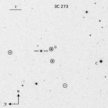
3C 273 has 297 $V$-band photometric epochs, and their magnitudes were calibrated by differential photometry using the star C in Figure 1 (see more details in Smith et al. 1985). The $V$-band light curve from SO is shown in the following Section 3.3.

Figure 1: The field around 3C 273. Star C ($V=11.87$; Smith et al., 1985) is used as the spectrophotometric standard star for the SO observation. Star G was used as the spectroscopic comparison star for the observations from Lijiang Observatory, while stars in circle were used to calibrate the Lijiang photometry. Here, we just adopt the same historical designation of “C” and “G” in Smith et al. (1985).

For the 374 spectroscopic observations, there are only 291 spectra that have the photometric observations in the same nights. They were calibrated using the corresponding photometric magnitudes, and are used in the following analysis. After combining the exposures in the same night, there are totally 283 spectroscopic epochs. The other 83 spectra with no simultaneous photometric observations are not used in this paper.

It should be noted that the aperture used in the spectroscopic observation includes almost all of the starlight from the host galaxy and the host contribution in the aperture is less than 6% (estimated from the image fitting in Section 6.2.3). Thus, the night-to-night calibration should not be significantly influenced by the host contribution in the different apertures used in the spectroscopy and photometry. The consistency of the SO and Lijiang light curves in the following Section 3.3 also supports that.

Table 1: Continuum and emission-line fluxes of 3C 273

Spectra							Photometry
JD	$F_{5100}$	$F_{\rm H\beta}$	$F_{\rm H\gamma}$	$F_{\rm Fe}$	Obs.		JD ($V$)	Mag ($V$)	Obs.
2454795.02	$21.75\pm 0.27$	$18.17\pm 0.24$	$6.93\pm 0.13$	$14.95\pm 0.28$	S		2454795.01	$12.71\pm 0.02$	S
2454800.99	$22.95\pm 0.28$	$18.27\pm 0.25$	$6.70\pm 0.16$	$15.41\pm 0.34$	S		2454801.00	$12.68\pm 0.02$	S
2454802.99	$24.09\pm 0.27$	$18.00\pm 0.23$	$6.27\pm 0.12$	$15.11\pm 0.27$	S		2454802.99	$12.66\pm 0.02$	S
2454803.97	$22.28\pm 0.27$	$16.92\pm 0.23$	$5.90\pm 0.11$	$14.41\pm 0.25$	S		2454804.04	$12.74\pm 0.02$	S
2454828.98	$20.40\pm 0.27$	$17.64\pm 0.23$	$6.02\pm 0.11$	$14.93\pm 0.24$	S		2454804.05	$12.70\pm 0.02$	S

Note. — $F_{5100}$ is the continuum flux at 5100Å in units of ${\rm 10^{-15}erg\,s^{-1}cm^{-2}\AA^{-1}}$. The emission-line flux is given in units of ${\rm 10^{-13}erg\,s^{-1}cm^{-2}}$. Obs. is the observatory, “S” $=$ SO, “L” $=$ Lijiang, and “A” $=$ ASAS-SN. This table is available in its entirety in a machine-readable form in the on-line journal. A portion is shown here for guidance regarding its form and content.

2.2 SEAMBH Campaigns of the Lijiang 2.4m telescope

As a candidate for super-Eddington accreting massive black holes (SEAMBHs), 3C 273 was selected as a target in our SEAMBH campaign (Du et al., 2014, 2015, 2016b, 2018b; Wang et al., 2014) for cosmology (Wang et al., 2013). We monitored 3C 273 from December 28, 2016 to June 13, 2017 using the 2.4 m telescope at the Lijiang Station of the Yunnan Observatories, Chinese Academy of Sciences. It is mounted with the Yunnan Faint Object Spectrograph and Camera (YFOSC), which is a multi-functional instrument both for photometry and spectroscopy. The YFOSC detector is a ${\rm 2k\times 4k}$ back-illuminated CCD with pixel size of 13.5$\,{\rm\mu m}$, providing a ${\rm 10^{\prime}\times 10^{\prime}}$ field of view (${\rm 0^{\prime\prime}.283}$ per pixel). Grism 14 and a $2^{\prime\prime}.5$-width slit were used, which provide a spectral dispersion of ${\rm 1.74\,\AA\,pixel^{-1}}$ and a resolution of $\sim$ 500 km/s (Du et al., 2016a). The wavelength coverage is 3800–7200Å, and the wavelength was calibrated by neon and helium lamps. The spectra were reduced using the standard IRAF v2.16 procedures.

We adopted the calibration approach based on in-slit comparison star (e.g., Maoz et al., 1990; Kaspi et al., 2000; Du et al., 2014, 2018b) rather than the [O iii]-based approach (e.g., van Groningen & Wanders, 1992; Peterson et al., 2013; Barth et al., 2015; Fausnaugh, 2017) for the spectroscopic observation. We observed 3C 273 and a nearby comparison star (star G in Figure 1) simultaneously by rotating the long slit, and used the comparison star as a standard to do the calibration. The fiducial spectrum of the comparison star is generated by averaging the spectra observed in photometric conditions. This approach ensures highly accurate relative flux calibration with a precision of $\sim 2\%$ (Du et al., 2014, 2018b; Lu et al., 2016).

We also performed photometric observations using the Johnson $V$ filter. The light curve of 3C 273 in $V$-band is measured by differential photometry using 4 stars (the circled stars in Figure 1) in the same field. There are 28 photometric and 27 spectroscopic epochs in Lijiang observations, respectively. The average sampling interval is $\sim 6$ days. The photometric light curve from Lijiang, which has been scaled to match the SO $V$-band light curve, is shown in Section 3.3.

2.3 All-Sky Automated Survey for Supernovae project

For comparison, we also show the $V$-band light curve of 3C 273 from the All-Sky Automated Survey for Supernovae (ASAS-SN) project . The ASAS-SN project (Shappee et al., 2014; Kochanek et al., 2017) is working toward imaging the entire sky every night down to $V\sim 17$ magnitude, and spans $\sim 2-5$ years with $\sim 100-400$ observational epochs for different objects. The ASAS-SN light curve of 3C 273 used here consists of 348 epochs in a 6-year period after averaging multiple observations obtained within a night. The ASAS-SN $V$-band light curve, after scaling to the SO light curve, is provided in the following Section 3.3.

3 measurements

3.1 Mean and RMS spectra

Small wavelength shifts in the spectra, which average to about 1.4Å for the SO data and 1.2Å for the Lijiang data, caused by instrument flexure, uncertainties in the wavelength calibration, and any mis-centering of the object within the slit have been corrected by aligning all spectra to [O iii]$\lambda 5007$. In addition, correction for the Galactic extinction of $A_{V}=0.057$ has been applied to the spectra (Cardelli et al., 1989; Schlafly & Finkbeiner, 2011).

Figure 2: Mean and RMS spectra of 3C 273 (observed flux vs. rest-frame wavelength).

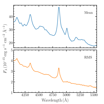
To show the general properties of the spectra and evaluate the variations at different velocities, we plot the mean and the root-mean-square (RMS) spectra in Figure 2. The definitions of the mean and RMS spectra are

$$\bar{F}_{\lambda}=\sum_{i=1}^{N}F_{\lambda}^{i}/N$$ (1)

and

$$S_{\lambda}=\left[\sum_{i=1}^{N}\left(F_{\lambda}^{i}-\bar{F}_{\lambda}\right)^{2}/N\right]^{1/2},$$ (2)

respectively, with $N$ being the total number of spectra, and $F_{\lambda}^{i}$ being the $i$-th spectrum. The strong signatures of emission lines in the RMS spectrum indicate that their variations are significant.

3.2 Light curves

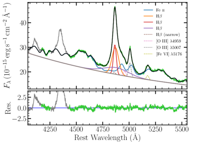
We use the multi-component spectral fitting approach to measure the light curves of the emission lines (e.g., Barth et al., 2013; Hu et al., 2015, 2016). The continuum is modeled with a power-law and the narrow emission-line components ([O iii]$\lambda\lambda 4959,5007$ and narrow H$\beta$) by a single Gaussian. The emission features of Fe ii are modeled using the template from Boroson & Green (1992). The profile of broad H$\beta$ line is modeled by 3 Gaussians. In addition, there are some other narrow emission lines in the optical Fe ii region (Vanden Berk et al., 2001). The high-S/N spectra of 3C 273 allow us to add extra line to improve the fitting, which can also compensate the potential inconsistency between the Fe ii of 3C 273 and the Fe ii template of I Zw 1 from Boroson & Green (1992). Similar to Hu et al. (2015), we add a coronal line [Fe vi]$\lambda 5176$ in our fitting. All of the narrow lines are fixed to have the same width and shift. The [O iii]$\lambda$4959 and the narrow H$\beta$ are fixed to have $1/3$ (Osterbrock & Ferland, 2006) and $1/10$ (Kewley et al., 2006; Stern & Laor, 2013) of the [O iii]$\lambda$5007 flux, respectively. We tried to fit the broad H$\beta$ using two Gaussians, but got poor fitting results with significant broad H$\beta$ signal in the residual spectra, which means two Gaussians are not enough to describe the H$\beta$ profile. Therefore, we changed to using three Gaussians in the fitting. The contribution of the host galaxy in the slit is estimated to be $\lesssim 6\%$ (estimated from our image fitting in Section 6.2.3), thus is ignored in the fitting. The fitting is performed mainly at 4430-5550Å (the H$\beta$ and Fe ii region), and the window 4170-4260Å is also added to constrain the continuum slope (Hu et al., 2008). We do not add the H$\gamma$ region in the fitting window in order to reduce the number of model components. An example of a fit is shown in Figure 3.

Figure 3: An example of the spectral fitting. The part of the spectrum included in the fitting is plotted in green, excluded part is marked in gray. The best-fit model (in black) is composed of the power-law continuum, Fe ii emission (blue line, using the template from Boroson & Green 1992), broad H$\beta$ (red, orange, and purple lines), and a group of narrow emission lines (dashed lines). The residual is shown in the bottom panel.

After subtracting the continuum, Fe ii, [O iii]$\lambda\lambda$4959,5007, and [Fe vi]$\lambda 5176$, the light curves of the H$\beta$ and H$\gamma$ emission lines are measured by integrating the fluxes of the residual spectra in the windows 4800-4920Å and 4280-4420Å in the rest frame, respectively. We do not subtract narrow H$\beta$ in the integration window; thus, the H$\beta$ light curve contains the contribution from its narrow component. Considering that the variability time scale of narrow line is much longer, it does not influence the lag measurement. The 5100Å continuum and the Fe ii (4434-4684Å) light curves are derived directly from the fitting results.

Spectra obtained in very poor weather conditions, or at extremely large airmasses are removed from the analysis. This includes 11 SO spectra and three spectra from Lijiang. In addition, some data points in the $V$-band light curve were edited out of the analysis for similar reasons and are colored gray in Figure 4. Error bars shown in the light curves contain both Poisson noise and systematic uncertainties. The systematic uncertainties are estimated by the median filter method (Du et al., 2014). We first smooth the light curve by a median filter with 5 points, and then subtract the smoothed light curve from the original one. The standard deviation of the residual is used as the estimate of the systematic uncertainty.

3C 273 emits strong radio and high-energy radiation (e.g., Courvoisier, 1998; Türler et al., 1999; Soldi et al., 2008). Fortunately, the contribution from the synchrotron light in the optical band is weak (Impey et al., 1989; Smith et al., 1993), which is also supported by the non-blazar-like flux variations in its optical band. Meanwhile, the SO polarimetry shows that its polarization (potentially produced by the synchrotron emission) remains exceptionally low, except at the beginning of the program.

Furthermore, the RMS spectrum in Figure 2 shows stronger signal in the blue part, which means 3C 273 is more variable at shorter wavelengths. This is also evidence for the dominant contribution from the accretion disk in the optical band, because the non-thermal emission from the jet is much redder. The photometric monitoring campaign from Zeng et al. (2018) also confirms this result. In addition, the variability analysis in Chidiac et al. (2016, 2017) did not show any correlation between the optical/IR and the radio/X-ray/$\gamma$-ray emission, which also suggests the optical flux is dominated by the thermal emission from the accretion disk. Only a few flare-like events are found in the $V$-band light curve (e.g., Julian date 100 and 580, from the zero point of 2454700 in Figure 4), but they do not cause serious disruption to the time-series analysis. Therefore, the jet emission of 3C 273 does not influence the lag measurements in the following sections.

Figure 4: Light curves and CCFs. The left panels are the light curves of the $V$-band, the continuum at 5100Å, and the various emission lines. The $V$-band light curve was observed by SO, ASAS-SN, and Lijiang. 11 points in gray are removed in the time-series analysis of this paper (see more details in Section 3.2). The $F_{5100}$ light curve is in units of ${\rm{10}^{-15}erg\,s^{-1}\,{cm}^{-2}\,\AA^{-1}}$, and emission-line fluxes are in ${\rm{10}^{-13}erg\,s^{-1}\,{cm}^{-2}}$. Here Fe ii  is the blue blend from 4430Å to 4680Å. The gray dashed line in the 5100Å light curve is the linear fit for detrending. The black points in panels b-f are obtained from Lijiang after the inter-calibration (see Section 3.3). All of the other spectroscopic data points are from the SO observations. In the right panels, black curves denote the CCFs (or ACFs). Blue histograms show the corresponding CCCD. The CCFs are obtained from $F_{5100}$ (after detrending) and the corresponding emission-line light curves. The January 1 of each year is marked on the time axis of the upper panel.

3.3 Inter-calibration

Because of the different apertures used for the SO, Lijiang, and ASAS-SN observations, inter-calibration of the three light curves is necessary. We adopt the method used by Peterson et al. (1991) to scale the Lijiang light curve to match the SO light curve. For the continuum, we assume

$$F_{\mathrm{S}}(\mathrm{5100\mbox{\AA}})=\varphi_{5100}F_{\mathrm{L}}(\mathrm{5100\mbox{\AA}})-G_{0},$$ (3)

where $G_{0}$ is a constant to account for the difference in the contribution of the host galaxy (aperture effect), $\varphi_{5100}$ is a scale factor, $F_{\mathrm{S}}(\mathrm{5100\mbox{\AA}})$ and $F_{\mathrm{L}}(\mathrm{5100\mbox{\AA}})$ are the 5100Å continuum fluxes of adjacent epochs ($<$ 4 day apart) of the SO and Lijiang observations. For the Balmer lines and Fe ii emission, we assume

$$F_{\rm S}({\rm line})=\varphi_{\rm line}F_{\rm L}({\rm line}),$$ (4)

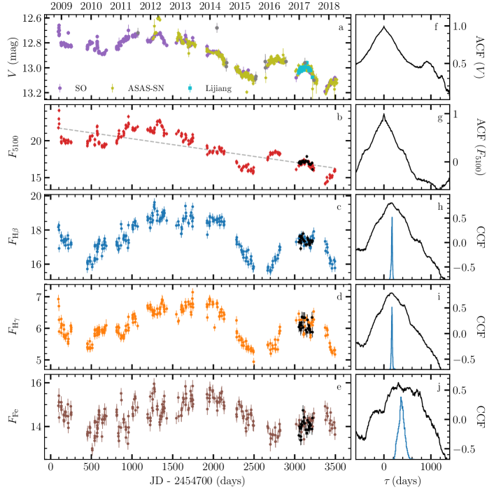
where “line” refers to the relevant emission line, $\varphi_{\rm line}$ is the scale factor, and $F_{\rm S}$ and $F_{\rm L}$ are the emission-line fluxes measured for epochs $<$ 4 days apart. Considering that the central wavelength of H$\beta$ is not far from 5100Å, we assume $\varphi_{\rm H\beta}=\varphi_{5100}$. Using the Levenberg-Marquardt algorithm (Press et al., 1992), the best-fit values are $\varphi_{5100,\rm H\beta}=0.9986$, $\varphi_{\rm H\gamma}=1.0571$, $\varphi_{\rm FeII}=0.9906$, and $G_{0}={\rm 0.02\times 10^{-15}}$ ${\rm erg\ s^{-1}\ cm^{-2}\ \mbox{\AA}^{-1}}$. The small value of $G_{0}$ indicates that the aperture effect with respect to the host galaxy contribution to the spectrum is negligible and that the overall contamination by the host galaxy to the data is weak (see Section 2.1). The calibrated light curves are shown in Figure 4 and provided in Table 1. Similarly, the ASAS-SN and Lijiang $V$-band light curves shown in Figure 4 have also been scaled to match the SO $V$-band light curve.

4 Analysis

4.1 Variability characteristics

The $F_{\rm var}$ parameter (Rodríguez-Pascual et al., 1997; Edelson et al., 2002) is adopted to quantify the variability amplitude of the light curve. It is defined as

$$F_{\rm var}=\frac{\left(\sigma^{2}-\Delta^{2}\right)^{1/2}}{\langle f\rangle},$$ (5)

where $\langle f\rangle$ is the mean flux in the light curve, $\sigma$ is the square root of the variance

$$\sigma^{2}=\frac{1}{N-1}\sum_{i=1}^{N}\left(f_{i}-\langle f\rangle\right)^{2},$$ (6)

and $\Delta^{2}$ is the mean square value of the uncertainties $\Delta_{i}$

$$\Delta^{2}=\frac{1}{N}\sum_{i=1}^{N}\Delta_{i}^{2}.$$ (7)

The $F_{\rm var}$ of each light curve is listed in Table 2. The variation amplitudes of the continuum and H$\beta$ fluxes are 10.9% and 5.2%, respectively. In addition, we also list $R_{\rm max}$ in Table 2, which is defined as the ratio of the maximum to the minimum in the light curve, as well as the median values of the light curves and their standard deviations.

Table 2: Light Curve Statistics

Lines	Median Flux	$F_{\rm var}(\%)$	$R_{\rm max}$
H$\beta$	$17.40\pm 0.94$	$5.24\pm 0.23$	1.23
H$\gamma$	$6.02\pm 0.47$	$7.44\pm 0.33$	1.32
Fe ii	$14.44\pm 0.61$	$3.81\pm 0.19$	1.18
$F_{5100}$	$19.46\pm 2.09$	$10.88\pm 0.45$	1.51

Note. — The emission-line fluxes and 5100Å  continuum are in units of ${\rm 10^{-13}\,erg\,s^{-1}\,cm^{-2}}$ and ${\rm 10^{-15}\,erg\,s^{-1}\,cm^{-2}\,\AA^{-1}}$, respectively. The flux, $F_{\rm var}$, and $R_{\rm max}$ of the $F_{5100}$ light curve are measured in the observed frame (with Galactic extinction correction).

4.2 Time lags

The continuum light curve of 3C 273 shows long-term variations that do not appear in the emission-line light curves (see Figure 4). This long-term trend may bias the lag detection, and thus we “detrend” the 5100Å light curve by subtracting a linear fit before the lag measurement (suggested by Welsh 1999, see also, e.g., Peterson et al. 2004; Denney et al. 2010). This fit is shown in Figure 4. The detrending improves the correlation coefficients in the following cross-correlation analysis. We tried to detrend the emission-line light curves, but the slopes of their linear fits are all close to zero within 3-$\sigma$ uncertainties. Therefore, we only detrend the 5100Å light curve.

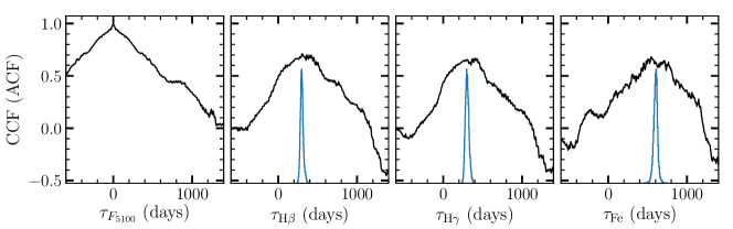
We adopt the interpolated cross-correlation function (ICCF; see Gaskell & Sparke, 1986; Gaskell & Peterson, 1987; White & Peterson, 1994) to measure the time lags of the emission lines relative to the variation of the continuum at 5100Å after detrending. The centroid of the CCF above a typical value (80%) of the maximum correlation coefficient ($r_{\rm max}$) is used as the lag measurement.

The uncertainties of the time lags are obtained through the “flux randomization/random subset sampling (FR/RSS)” method (Maoz et al., 1990; Peterson et al., 1998, 2004), which both randomizes the measured fluxes based on their uncertainties and resamples the light curves. The resampling is performed by randomly selecting $N$ points from the light curve (redundant selection is allowed), where $N$ is the total number of epochs in the light curve. A subsample is constructed after ignoring the redundant points (roughly a fraction of $\sim 0.37$). We repeat this process 10000 times and obtain the cross-correlation centroid distribution (CCCD) by performing CCF to the light-curve subsamples. It is similar to the so-called “bootstrapping” technique. Then the values of the time lags and the corresponding uncertainties are obtained from the median, 15.87%, and 84.13% ($1\sigma$) quantiles of the CCCD.

The auto-correlation functions (ACFs), CCFs, and CCCDs between the emission-line light curves and the detrended 5100Å light curve are shown in the right panels of Figure 4. We also provide the results without the detrending in Appendix. The time lags of the emission lines are listed in Table 3. The time lag of the H$\beta$ emission line is $146.8^{+8.3}_{-12.1}$ days in the rest frame, consistent with the lag found for the H$\gamma$ line. The response of Fe ii to continuum variations is found to be nearly a factor of 2 longer than that of the Balmer lines, at $322.0^{+55.5}_{-57.9}$ days in the rest frame. The lag uncertainties in our measurements are smaller than those in Kaspi et al. (2000), because of our denser sampling cadence, higher S/N ratios, and longer monitoring period.

Figure 5: Time lag ratio of Fe ii to H$\beta$ vs. their intensity ratio. The orange triangles show the two objects in Barth et al. (2013). The blue circles are the objects presented in Hu et al. (2015).

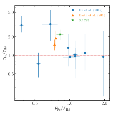
Hu et al. (2015) show a tentative correlation between the time lag ratio ($\tau_{\rm Fe}/\tau_{\rm H\beta}$) and the intensity ratio ($F_{\rm Fe}/F_{\rm H\beta}$) of the Fe ii and H$\beta$ lines. The Fe ii lag is similar to the H$\beta$ lag if $F_{\rm Fe}/F_{\rm H\beta}\gtrsim 1$, while the Fe ii lag tends to be longer if $F_{\rm Fe}/F_{\rm H\beta}<1$. The Fe ii and H$\beta$ time lags of 3C 273 are in good agreement with the $\tau_{\rm Fe}/\tau_{\rm H\beta}$ – $F_{\rm Fe}/F_{\rm H\beta}$ correlation (Figure 5).

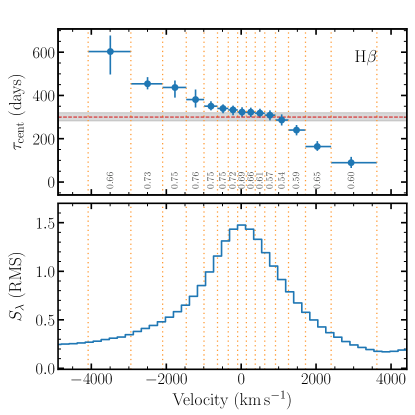
4.3 Velocity-resolved lags of H$\beta$

We use velocity-resolved RM to investigate the geometry and kinematics of the BLR in 3C 273. The H$\beta$ line is divided into 15 velocity bins, with each bin having the same flux as in the RMS spectrum created after the subtraction of continuum, Fe ii, and narrow lines in Section 3.2 (e.g., Bentz et al., 2008; Denney et al., 2010; Grier et al., 2013; Du et al., 2016a; De Rosa et al., 2018). The fluxes in each bin are integrated to generate light curves that are used to cross-correlate with the 5100Å variations (after detrending). The time lag and the associated uncertainties of each bin are obtained using the same method described in Section 4.2.

Figure 6: Velocity-resolved time lags of the H$\beta$ line in the observed frame. The top panel shows the centroid time lags and their uncertainties in velocity bins denoted by the vertical dotted lines. The horizontal dashed line and the shadowed region are the mean time lag and its associated 1-$\sigma$ uncertainties. The gray numbers in the top panel are the maximum correlation coefficients of the CCFs in the velocity bins. The RMS spectrum is shown in the bottom panel in units of ${\rm 10^{-15}\,erg\,s^{-1}\,cm^{-2}\,\AA^{-1}}$.

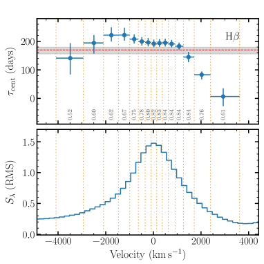
We plot the velocity-resolved time lags (in the observed frame) in Figure 6. The maximum correlation coefficients for individual bins are also shown in Figure 6. The velocity-resolved result shows a complex structure. In general, the lags are longer at small velocities and shorter at high velocities, which is the signature of a Keplerian disk or virialized motion. However, the lags at the blue velocities are systematically longer than those in the red wing. There are at least several possibilities: (1) a classic explanation is that the H$\beta$-emitting gas has some inflowing radial velocity (e.g., Bentz et al., 2008; Denney et al., 2010; Grier et al., 2013; Du et al., 2016a; De Rosa et al., 2018); (2) a rotating disk wind model suggested by Mangham et al. (2017) can produce the velocity-resolved lags resembling the “red-leads-blue” inflow signature; and (3) the BLR gas is located in an eccentric or lopsided disk, and shows net velocity along the line of sight. The BLR dynamical modeling technique (e.g., Pancoast et al., 2011, 2012; Grier et al., 2017; Williams et al., 2018) is required to investigate the geometry and kinematics of the BLR of 3C 273 in more detail in the future.

Table 3: Emission-line Time Lags

Lines	$r_{\rm max}$	lags (days)
		observed frame	rest frame
H$\beta$	0.81	$170.0_{-14.0}^{+9.6}$	$146.8_{-12.1}^{+8.3}$
H$\gamma$	0.79	$169.7_{-11.2}^{+10.2}$	$146.5_{-9.7}^{+8.8}$
Fe ii	0.63	$373.0_{-67.1}^{+64.3}$	$322.0_{-57.9}^{+55.5}$

4.4 Line widths

We investigate the behavior of the broad emission-line profiles of H$\beta$ and H$\gamma$ through the measurement of the FWHM and the line dispersion ($\sigma_{\rm line}$). The line dispersion is defined as

$$\sigma_{\rm line}^{2}(\lambda)=\left<\lambda^{2}\right>-\lambda_{0}^{2},$$ (8)

where $\lambda_{0}=\int\lambda f(\lambda)d\lambda/\int f(\lambda)d\lambda$ is the flux-weighted centroid wavelength of the emission line profile, $\left<\lambda^{2}\right>=\int\lambda^{2}f(\lambda)d\lambda/\int f(\lambda)d\lambda$, and $f(\lambda)$ is the flux density. Line widths are measured from the line profiles in the mean and RMS spectra after subtraction of the continuum, Fe ii emission, and narrow emission lines. The uncertainties of the line widths are estimated by the bootstrap method (Peterson et al., 2004). We randomly select $N$ spectra with replacement (redundant selection is allowed, $N$ is the total number of spectra for 3C 273), and construct a spectral subset after removing the redundant spectra. Then, the mean and RMS spectra are generated from the subset, and are used to measure the line widths. This process is repeated 10000 times to create the line width distributions. The standard deviations of the FWHM and $\sigma_{\rm line}$ distributions are regarded as the uncertainties.

The line widths of H$\beta$ and H$\gamma$ are calculated separately for the SO and Lijiang data. To estimate the spectral broadening caused by the instruments and seeing, we compare our spectra with higher-resolution spectra obtained with an instrument with a well-understood line spread function. In this case, we use the o44301010 and o44301020 observations of 3C 273 made by STIS aboard the Hubble Space Telescope (Hutchings et al., 1998). The spectral broadening of SO and Lijiang are $1157\pm 46$ km/s and $485\pm 38$ km/s, respectively. After subtracting the spectral broadening in quadrature, the line widths of the H$\beta$ and H$\gamma$ lines are listed in Table 4. For the SO spectra, the FWHM of H$\beta$ and H$\gamma$ are both around $\sim$3300 km/s. We adopt the FWHM from the mean spectrum to calculate of BH mass in the following sections, because the $\sigma_{\rm line}$ measurement is sensitive to the wings of the emission line and the accuracy of the continuum subtraction. The FWHM of Fe ii is 2142.4$\pm$116.1 km/s, which is obtained directly from the fitting. Compared with the H$\beta$ and H$\gamma$, the FWHM of Fe ii is significantly narrower. This suggests that the Fe ii-emitting region is farther away from the BH than the region in the BLR producing the Balmer emission.

Table 4: Emission-line Widths

	Lines	Line width (mean)			Line width (RMS)
		FWHM (${\rm km\,s^{-1}}$)	$\sigma_{\rm line}$ (${\rm km\,s^{-1}}$)		FWHM (${\rm km\,s^{-1}}$)	$\sigma_{\rm line}$ (${\rm km\,s^{-1}}$)
Steward	H$\beta$	$3314.1\pm 59.3$	$1698.8\pm 25.1$		$1941.4\pm 69.5$	$1098.9\pm 39.9$
	H$\gamma$	$3313.8\pm 59.2$	$1667.7\pm 25.2$		$2439.1\pm 82.5$	$1444.5\pm 46.4$
	Fe ii	$2142.4\pm 116.1$	$\cdots$		$\cdots$	$\cdots$
Lijiang	H$\beta$	$3196.9\pm 39.2$	$1702.9\pm 16.5$		$3305.2\pm 420.1$	$1081.0\pm 238.8$
	H$\gamma$	$3139.0\pm 40.5$	$1535.9\pm 19.6$		$4079.7\pm 509.2$	$1176.9\pm 260.8$
	Fe ii	$2039.3\pm 70.6$	$\cdots$		$\cdots$	$\cdots$

Figure 7: Variability of the H$\beta$ profile in 3C 273. Two measures of the H$\beta$ width from SO are plotted with respect to time over a period of almost 10 years. The error bars of the line widths are estimated by the median filter method (see more details in Section 3.2).

Figure 8: Emission-line width of H$\beta$ as a function of its flux (for the SO program). The orange lines are the best fits to the data. The error bars of the line widths are same as in Figure 7.

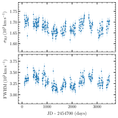
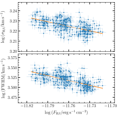
The FWHM and $\sigma_{\rm line}$ of individual spectra are also measured to investigate the line width changes during the campaign. After correcting for spectral broadening, the FWHM and $\sigma_{\rm line}$ of H$\beta$ from SO for the entire monitoring period are shown in Figure 7. Figure 8 plots the correlation between H$\beta$ emission-line flux and line width. There is a strong anti-correlation between line flux and width in H$\beta$ (Pearson’s coefficient and the null probability are $-0.59$ and $3.8\times 10^{-27}$ for FWHM vs. $F_{\rm H\beta}$, and are $-0.54$ and $4.5\times 10^{-22}$ for $\sigma_{\rm line}$ vs. $F_{\rm H\beta}$, respectively.) To quantify the correlation, we perform the linear regression of

$$\log V_{\rm H\beta}=\alpha+\beta\log F_{\rm H\beta},$$ (9)

where $V_{\rm H\beta}$ is $\rm FWHM_{H\beta}$ or $\sigma_{\rm H\beta}$. The uncertainties of the parameters are obtained using the bootstrap technique. The results are shown in Figure 8. The best-fit values for ($\alpha$, $\beta$) are ($-1.28\pm 0.37$, $-0.41\pm 0.03$) and ($1.46\pm 0.15$, $-0.15\pm 0.01$) for flux versus FWHM and $\sigma_{\rm H\beta}$, respectively. Similar correlations are reported for some other objects (e.g., Barth et al., 2015).

4.5 Line width versus lags

The RM campaign of 3C 273 performed by the International Ultraviolet Explorer (IUE) yielded time lags of $\tau_{\rm{\rm Ly\alpha}+N{\sc v}}=435_{-77}^{+77}$ and $\tau_{\text{C~{}{\sc iv}}}=690_{-106}^{+102}$ days in the rest frame for Ly$\alpha$ + N v and C iv lines relative to the UV continuum variation (Paltani & Türler 2005). The echo of the Ly$\alpha$ + N v lines with respect to the UV continuum is quite good with $r_{\rm max}\approx 0.6$, but the C iv response remains largely uncertain. Paltani & Türler (2005) took the centroid lag above $0.6\,r_{\rm max}$ of the Ly$\alpha$ + N v CCF as the lag measurement. For comparison to our optical measurements, we re-calculated their Ly$\alpha$ + N v lag using the $0.8\,r_{\mathrm{max}}$ criterion. There are multiple peaks in the ultraviolet CCF, and we only adopt the highest peak in the calculation. The re-determined Ly$\alpha$ + N v lag is $\tau_{\rm Ly\alpha+N{\sc v}}=72.2_{-23.5}^{+58.1}$ days in the rest frame. We plot the correlation between the lags and the FWHMs both for the UV and optical lines in Figure 9 , where it is seen that ${\rm FWHM}\propto\tau^{-0.55\pm 0.01}$ for the optical emission lines. This is similar to the results for NGC 5548 (Peterson & Wandel, 1999). This relation steepens to ${\rm FWHM}\propto\tau^{-1.1\pm 0.3}$ with the inclusion of the Ly$\alpha$ + N v lines.

Figure 9: Emission-line widths vs. their rest-frame time lags. The FWHM of Ly$\alpha$ + N v is taken from Paltani & Türler (2005), with the time lag recalculated in Section 4.5. The best linear fit for all emission lines is shown by the dotted line. The dashed line represents the best fit that omits Ly$\alpha$ + N v.

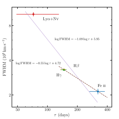
3C 273 shows a ${\rm FWHM}\propto\tau^{-0.56}$ relation for its optical emission lines that the UV emission lines do not follow. It implies that the geometry or kinematics of the UV-emitting clouds are different from the optical-line region, i.e., their virial factors in the BH mass measurements should be very different. The optical emission lines are relatively closer to ${\rm FWHM}\propto\tau^{-0.5}$ relation (consistent with the velocity-resolved result that the kinematics in the H$\beta$ region is generally a Keplerian disk or virialized motion); thus, we prefer to estimate the BH mass based on those lines. Given that the IUE campaign was carried out more than a decade before the optical RM program, the steeper slope may also be caused by a physical change in the geometry and/or kinematics of the BLR.

5 Black hole mass and accretion rate

Combining the results for the time lag, $\tau_{\rm line}$, and the line width, $V_{\rm line}$, the BH mass can be estimated by

$$M_{\bullet}=f_{\rm BLR}\frac{R_{\rm BLR}V_{\rm line}^{2}}{G},$$ (10)

where $R_{\rm BLR}=c\tau_{\rm line}$ is the emissivity-weighted radius of the BLR, $V_{\rm line}$ is given by the FWHM or $\sigma_{\rm line}$, $c$ is the speed of light, $G$ is the gravitational constant, and $f_{\rm BLR}$ is the virial factor depending on the kinematics, geometry, and inclination angle of the BLR. In general, the average $f_{\rm BLR}$ can be estimated by comparing RM-based BH masses for AGNs with available bulge stellar velocity dispersions with BH masses predicted from the $M-\sigma$ relation of inactive galaxies (e.g., Onken et al., 2004; Ho & Kim, 2014; Woo et al., 2015; Park et al., 2012; Grier et al., 2013; Ho & Kim, 2014). Specifically, for FWHM of H$\beta$ measured from their mean spectra, Ho & Kim (2014) demonstrate that the $f_{\rm BLR}$ is $1.3$ for AGNs with classical bulges or elliptical host galaxies (see also Mejía-Restrepo et al. 2018).

Independent from the calibration based on the $M_{\bullet}-\sigma_{*}$ relation, the Bayesian-based BLR dynamical modeling method (Pancoast et al., 2011, 2012) has been adopted in recent years to provide $f_{\rm BLR}$ for individual AGNs with different BLR geometry and kinematics (e.g., Pancoast et al., 2014a, b, 2018; Grier et al., 2017; Li et al., 2013, 2018; Williams et al., 2018). The velocity-resolved time lags of 3C 273 show “red-leads-blue” signatures, which may arise from inflow kinematics (in Section 4.3). Virial factors for AGNs with inflowing signatures as derived from dynamical modeling are diverse and range from $0.58-3.98$ (Grier et al., 2017; Pancoast et al., 2014b), but they average close to the value found by Ho & Kim (2014). Thus, we simply adopt $f_{\rm BLR}=1.3$ to calculate the BH mass for 3C 273, but acknowledge that there is a large amount of uncertainty in the value of this parameter (we do not include the uncertainty of $f_{\rm BLR}$ in our mass calculation). Based on the measurements of $\tau_{\rm H\beta}=146.8_{-12.1}^{+8.3}$ days (in the rest frame) and ${\rm FWHM_{H\beta}}=3314.1\pm 59.3$ km/s, the BH mass of 3C 273 is $M_{\bullet}=4.1_{-0.4}^{+0.3}\times 10^{8}M_{\odot}$.

The relativistic jet is found to have an inclination of $10^{\circ}$ with a Lorentz factor of $\Gamma\approx 11$ (Davis et al., 1991; Abraham & Romero, 1999), which is nicely agreeable with the measurements ($i=12^{\circ}\pm 2^{\circ}$) of the GRAVITY (see Section 6.1), showing that the BLR and the jet are perpendicular to each other (Gravity Collaboration et al., 2018). Since $\Theta_{\rm BLR}\approx 45^{\circ}$, the inclination ($12^{\circ}$) implies that the present estimate of SMBH mass is less affected by inclinations since the normalization factor $f_{\rm BLR}\propto\left[(H_{\rm BLR}/R)^{2}+\sin^{2}i\right]^{-1}$ is dominated by the geometric factor of $H_{\rm BLR}/R$ (i.e., $H_{\rm BLR}/R=\tan\Theta_{\rm BLR}$, where $H_{\rm BLR}$ is the half-thickness of the BLR).

The GRAVITY observations provide an SMBH mass of $M_{\bullet}=(2.6\pm 1.1)\times 10^{8}M_{\odot}$ (Gravity Collaboration et al., 2018), which is consistent with the present results within the uncertainties. We would like to point out that the most uncertainties of SMBH masses from Eq. (10) are due to $f_{\rm BLR}$. Detailed modelling BLR through Markov Chain Monte Carlo (MCMC) simulations can be done for the mass as well as the BLR geometry (Pancoast et al., 2011, 2014a; Li et al., 2013, 2018) independent of this factor. Application of the MCMC technique to 3C 273 will be carried out separately (Li et al. 2019 in preparation).

We use the equation for the dimensionless accretion rate of

$$\dot{\mathscr{M}}_{\bullet}=20.1\,\left(\frac{\ell_{44}}{\cos i}\right)^{3/2}m_{7}^{-2},$$ (11)

(e.g., Du et al., 2014) to find $\dot{\mathscr{M}}_{\bullet}=\dot{M}_{\bullet}/L_{\rm Edd}c^{-2}\approx 9.6$ in 3C 273, where $L_{\rm Edd}$ is the Eddington luminosity, $i(=12^{\circ})$ is the disk inclination angle, $\ell_{44}=L_{5100}/10^{44}{\rm erg~{}s^{-1}}=84.3$, and $m_{7}=M_{\bullet}/10^{7}M_{\odot}=41.0$. Using the bolometric luminosity for 3C 273 of $L_{\rm bol}\approx 1.3\times 10^{47}{\rm erg~{}s^{-1}}$ determined by Shang et al. (2005) (The luminosity has been transformed to the value corresponding to the cosmological parameters used in this paper), we find that $L_{\rm bol}/L_{\rm Edd}\approx 2.4$, indicating that the BH is accreting in this quasar at a mildly super-Eddington rate.

Table 5: Comparison of the RM-campaigns

	Cadence		Length	$N_{\rm spec}$
	Obs. season	Entire	(start$-$end yr)
	(days)	(days)	(days)
Kaspi et al. (2000)	40.3	66.8	2606 (1991-98)	39
This campaign	7.4	12.5	3400 (2008-18)	296

Note. — “Obs. season” cadence means that it is averaged only during observable seasons and the entire one does that it is averaged for the entire campaign. Length refers to the total period from the start to end. $N_{\rm spec}$ is the number of spectra taken from the corresponding campaigns.

6 discussion

6.1 Comparing with the previous and the GRAVITY results

Before the present work, Kaspi et al. (2000) made a mapping measurement of 3C 273 through a 7-year campaign of the Bok telescope and the Wise 1m telescope. They obtained the centroid lags of reverberation of the Balmer lines, $(R_{\rm H\alpha},R_{\rm H\beta},R_{\rm H\gamma})=(514_{-64}^{+65},382_{-96}^{+117},307_{-86}^{+57})$ltd, respectively, that are twice more as long as the present results. But the error bars of the present measurements are much smaller than those given by Kaspi et al. (2000). Peterson et al. (2004) revisited the data of Kaspi et al. (2000) and found $R_{\rm H\beta}=306.8_{-90.9}^{+68.5}$ltd, it is still double the present measured result in this paper. A brief comparison of the two campaigns is given by Table 5, showing that the present campaign has a much higher cadence than Kaspi et al. (2000). Considering the BLR dynamical timescales of $\tau_{\rm BLR}\approx R_{\rm BLR}/V_{\rm FWHM}=37.4\,R_{150}V_{3300}^{-1}$ yrs, the BLR cannot change by a factor of 2 in the last 27 yrs (since 1991), where $R_{150}=R_{\rm BLR}/150$ltd and $V_{3300}=V_{\rm FWHM}/3300{\rm km\,s^{-1}}$. Moreover, variations of the 5100Å  luminosity are about $\Delta L/L_{5100}\lesssim 1/4$ during the two campaigns and thus the difference of H$\beta$ lags measured by the campaigns is not caused by luminosity changes. The present measurements are more robust and reliable.

Very recently, the GRAVITY instrument installed on the Very Large Telescope Interferometer (VLTI) found a flatten disk structure of the BLR in 3C 273 with a half-opening angle of $\Theta_{\rm BLR}={45^{\circ}}_{-6}^{+9}$ and an emissivity-averaged radius of the Paschen-$\alpha$ emission region $R_{\rm Pa\alpha}=145\pm 35$ltd (Gravity Collaboration et al., 2018). It is exciting to find that $R_{\rm Pa\alpha}=R_{\rm H\beta}=R_{\rm H\gamma}$ holds within their error bars as listed in Table 3. This lends a robust demonstration that RM measurements are very reliable to spatially resolve compact regions in time domain through small telescopes.

Moreover, the opening angle of the geometrically thick BLR in 3C 273 might agree with that of the dusty torus. This is helpful to understand the hypothesis that the BLR-clouds are supplied by tidally captured clumps from the torus (Wang et al., 2017). In principle, the torus opening angles can be estimated by infrared emission as the reprocessed emission of optical and UV luminosities (Wang et al., 2005; Cao, 2005; Maiolino et al., 2007), but the infrared emissions in 3C 273 could be seriously contaminated by non-thermal emission from the jet. So it’s hard to estimate the opening angle of the torus in this way. Fortunately, the [O iii]  luminosity is $L_{\rm[O\,III]}\approx 1.5\times 10^{43}\rm erg\,s^{-1}$ from this campaign, allowing an estimate of the torus half-opening angle of $\Theta_{\rm torus}\approx 30^{\circ}\pm 10^{\circ}$ from the correlation between type 2 quasar ratio and [O iii]  luminosity (i.e., the receding torus model, e.g. Fig. 12 in Reyes et al., 2008). This shows potential evidence for the hypothesis of the physical connection between the BLR and the torus. The GRAVITY observation of the torus in 3C 273 in the future, as done in NGC 1068 (Jaffe et al., 2004), will directly measure the torus geometry to check if the geometrically-thick BLR matches that of the dusty torus. This will observationally justify the hypothesis of the BLR origin from the failed outflows of the outer part accretion disk (Czerny & Hryniewicz, 2011) or from torus (Wang et al., 2017).

6.2 Host galaxy

Figure 10: GALFIT decomposition for 3C 273. The upper panels show the fitting result in F105W filter. The lower panels show the fitting result in F547M filter. In each row, 1D profile, 2D image of the original data, the best-fit model for the host (the AGN is excluded to better highlight the host) and the residuals images are displayed. The 1D azimuthally averaged profile shows the original data (black dots), the best fit (violet solid line), and the subcomponents (PSF in dark blue dot-dashed line and bulge in red dashed lines). The axes of the images are in units of arcseconds. All images are on an asinh stretch.

6.2.1 Data

AGNs show strong correlations with their host galaxies, for example, the BH mass is strongly correlated with the mass of the galactic bulge of the host (e.g., Magorrian et al., 1998; Kormendy & Ho, 2013). To derive the bulge mass in 3C 273, we analyze its HST/WFC3 images, which were observed on March 17, 2013 (GO-12903, PI: Luis C. Ho) with the F547M filter in the UVIS channel for 360 sec and with F105W filter in the IR channel for 147 sec. Two additional short F547M exposures for 18 sec and 6 sec were taken to warrant against saturation of the nucleus in the long exposure. These two filters were selected to mimic the $B$ and $I$ bands in the rest frame of 3C 273. To better sample the point-spread function (PSF), the long UVIS observation was taken with a three-point linear dither pattern, while the IR observation was taken with the four-point box dither pattern. To avoid overheads due to buffer dump, we employed the UVIS2-M1K1C-SUB 1k$\times$1k subarray for the UVIS channel and the IRSUB512 subarray for the IR channel, which results in a restricted field-of-view of 40$\times$40 arcsec and 67$\times$67 arcsec, respectively.

Because of the sparseness of field stars in the vicinity of 3C 273, the observations were conducted in GYRO mode, leading to a considerable degradation of the PSF of the dither-combined image generated from the standard data reduction pipeline. Instead, we use the DrizzlePac task AstroDrizzle (v1.1.16) to correct the geometric distortion, align the sub-exposures, perform sky subtraction, remove cosmic rays, and, finally combine the different exposures. The core of the AGN was severely saturated in the long F547M exposure, and it was replaced with an appropriately scaled version of the 6 sec short exposure. Because the PSF of HST/WFC3 is under-sampled, we broaden the science image and the PSF by a Gaussian kernel such that the final images are Nyquist-sampled (Kim et al., 2008a). This largely removes the sub-pixel mismatch of the core of the PSF.

Table 6: Fitted Model Parameters for HST Images

Filter	$m_{\rm nuc}$	$m_{\rm host}$	$R_{e}$	$n$	$\mu_{e}$	RMS.	$\chi^{2}/\nu$	${a}_{1}$
	(mag)	(mag)	(′′)		(mag arcsec-2)
(1)	(2)	(3)	(4)	(5)	(6)	(7)	(8)	(9)
F105W	$12.12\pm 0.03$	$14.87\pm 0.60$	$11.87\pm 5.76$	$4\pm 1$	$23.63\pm 0.80$	0.19	4.44	$-0.09\pm 0.07$
F547M	$12.69\pm 0.01$	$16.43\pm 0.71$	$11.87\pm 5.76$	$4\pm 1$	$25.19\pm 0.67$	0.22	0.77	$-0.09\pm 0.07$

Note. — Col. (1): HST filter. Col. (2): Apparent nuclear magnitude in the observed filter. Col. (3): Apparent host magnitude fitted by a Sérsic component in the observed filter. Col. (4): Effective radius of the host galaxy. Col. (5): Sérsic index for the host galaxy. Col. (6): Surface brightness of the host galaxy at the effective radius. Col. (7): RMS of the 1D profile residual in the source-dominated region. Col. (8): $\chi^{2}/\nu$ for the fit. Col. (9): Amplitude of the first Fourier mode, which is a measure of the lopsidedness of the galaxy.

6.2.2 Image decomposition

The F105W filter image for 3C 273 shows a dominant nucleus and a host galaxy with no clear disk component. The F547M filter image is considerably shallower. To extract quantitative measurements of the bulge, we use the program GALFIT (Peng et al., 2002, 2010) to fit two-dimensional surface brightness distributions to the HST images. A crucial ingredient is the PSF, which will have a strong effect on the brightness of the active nucleus. Unfortunately, no suitable bright star is available to be used as the PSF within the limited field-of-view of the subarray WFC3 images. Instead, we generated a high-S/N empirical PSF by combining a large number (24 for F105W and 12 for F547M) of bright, isolated, unsaturated stars observed in other WFC3 programs. Extensive tests, consisting of fits to isolated bright stars, indicate that our stacked empirical PSF is far superior to synthetic PSFs generated from the TinyTim program (Krist & Hook, 2008), and it has higher S/N than the PSFs of individual stars. The reduced chi-squared of the fits are $\sim$3 times larger for the TinyTim synthetic PSF. Comparison of empirical PSFs observed from different programs indicate that the WFC3 PSF does not vary significantly with time ($<$ 10%).

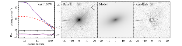
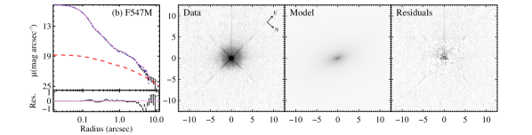
We first obtain the best global fit on the deeper F105W image, whose redder wavelength coverage is more sensitive to the host. Models consisting of two components are adopted, with a point source (represented by the PSF) for the nucleus, and the bulge parameterized by a Sérsic function (Sérsic, 1968) with index $n$. Models with $n\approx 3-5$ give the best fitting residuals. We adopt $n=4$ as the best model and include the difference between the $n=3$ and $n=5$ model into the uncertainty. Figure 10 summarizes the model fits in F105W and F547M filter for the $n=4$ model. We use the $m=1$ Fourier mode, which is sensitive to lopsidedness, to gauge the degree of global asymmetry of the galaxy (see, e.g., Kim et al., 2008b, 2017). Since the host is considerably weaker in the F547M image, it is fit by keeping the structural parameters fixed to the values obtained from the F105W model, solving only for the magnitudes of the nucleus and host.

The best-fit parameters are given in Table 6. For bright type 1 AGNs, such as 3C 273, the uncertainties are dominated by errors in the PSF adopted for the nucleus. We estimate the uncertainties in the PSF by generating variants of the empirical PSF by combining different subsets of stars, and then repeating the fit. Subtraction of the background can also affect the fit. We subtract $\pm 1\sigma$ of the background level from the image, and then take the mean of the differences relative to the fiducial value of the sky as the uncertainty. The uncertainties caused by the PSF, background subtraction, and the Sérsic index $n$ are all taken into account in the final error estimation.

6.2.3 Stellar mass

The GALFIT decomposition of the HST images yields F547M and F105W magnitudes for the bulge of the host galaxy of 3C 273. We convert these HST-based magnitudes into intrinsic, rest frame $I$-band magnitude and $B-I$ color, from which we can estimate the stellar mass following the prescriptions of Bell & de Jong (2001). To estimate the $K$-correction, we use Bruzual & Charlot (2003) models with solar metallicity, a Chabrier (2003) stellar initial mass function (IMF), and an exponentially decreasing star formation history with a star formation timescale of 0.6 Gyr to generate a series of template spectra with ages spanning 1 to 12 Gyr. After accounting for Galactic extinction and redshift, we convolve the spectra with the response functions of the HST filters to generate synthetic F547M and F105W magnitudes.

The observed host color is $\mathrm{F547M-F105W}=1.6\pm 0.9$. This color is best matched with a stellar population template of ${2.5}$ Gyr (the templates of 1 Gyr and 12 Gry for the lower and upper limits), resulting in $M_{I}=-24.3\pm 0.6$ and $B-I$ = $1.5\pm 1.0$. Following Bell & de Jong (2001) and the correction of Longhetti & Saracco (2009), we derive a stellar mass of $M_{*}=10^{11.3\pm 0.7}M_{\odot}$, assuming solar metallicity and a Chabrier IMF. The ratio of BH mass and spheroid is about $2.0\times 10^{-3}$, which agrees with the Magorrian relation (e.g., Kormendy & Ho, 2013).

7 summary

We present the results from a reverberation mapping campaign of 3C 273 from Nov 2008 to Mar 2018. Time lags relative to the observed continuum variations of the active nucleus of several emission lines were successfully detected, and we measure the velocity-resolved lags for the H$\beta$ line.

• The time lags of the H$\beta$ and H$\gamma$ emission lines are $(\tau_{\rm H\beta},\tau_{\rm H\gamma})=(146.8_{-12.1}^{+8.3},146.5_{-9.7}^{+8.8})$ days in the rest frame, which are very similar to each other.

• The Fe ii lines have a lag of $\tau_{\rm Fe}=322.0_{-57.9}^{+55.5}$ days in the rest frame, which follows the $\tau_{\rm Fe}/\tau_{\rm H\beta}-F_{\rm Fe}/F_{\rm H\beta}$ correlation found in Hu et al. (2015). The Fe ii and the Balmer line regions follow the virialized relation of $\tau\propto V_{\rm FWHM}^{-2}$, showing the stratified structures in space.

• The velocity-resolved lag measurements of the H$\beta$ line show a complex structure. The lags are longer at small velocities and shorter at high velocities, which is the signature of a rotation-dominated disk. In addition, the blue wing shows longer lags than those at red velocities. This may be explained by inflowing radial motions in the H$\beta$-emitting gas or some other special BLR kinematics.

• Along with the UV lines, we find that 3C 273 has a stratified structure in its BLR, with higher-ionization lines arising from inner regions but lower-ionization lines from the outer part. The UV lines deviate significantly from the ${\rm FWHM}\propto\tau^{-0.5}$ relation.

• Adopting a virial factor of $f_{\rm BLR}=1.3$, 3C 273 has a BH mass of $M_{\bullet}=4.1_{-0.4}^{+0.3}\times 10^{8}M_{\odot}$ and is accreting with a rate of $9.3\,L_{\rm Edd}\,c^{-2}$, indicating that the black hole is undergoing intermediate super-Eddington accretion.

• From decomposition of its HST images, we obtain a host stellar mass of $M_{*}=10^{11.3\pm 0.7}M_{\odot}$. We find that a ratio of BH mass and host spheroid ($2\times 10^{-3}$) follows the Magorrian relation.

Considering that the geometrically thick BLR of 3C 273 detected by the GRAVITY is roughly consistent with the torus obtained by the receding statistic, we expect to compare with torus structure spatially resolved by the VLTI in order to reveal the origin of BLR clouds, which is suggested to be supplied by the central black hole tidal capture of clumps from the torus (Wang et al., 2017).

We thank an anonymous referee for a helpful report. We acknowledge the support by National Key R&D Program of China (grants 2016YFA0400701 and 2016YFA0400702), by NSFC through grants NSFC-11873048, -11833008, -11573026, -11473002, -11721303, -11773029, -11833008, -11690024, and by Grant No. QYZDJ-SSW-SLH007 from the Key Research Program of Frontier Sciences, CAS, by the Strategic Priority Research Program of the Chinese Academy of Sciences grant No.XDB23010400. Data from the Steward Observatory spectropolarimetric monitoring project were used. This program is supported by Fermi Guest Investigator grants NNX08AW56G, NNX09AU10G, NNX12AO93G, and NNX15AU81G. We also acknowledge the support of the staff of the Lijiang 2.4m telescope. Funding for the telescope has been provided by CAS and the People’s Government of Yunnan Province.

For completeness, we also show the results of the time-series analysis and the velocity-resolved lag measurement without detrending in Figures 11 and 12. The time lags of the H$\beta$, H$\gamma$, and Fe ii  lines are listed in Table 7. The long-term variations in 5100Å light curve (i.e., the long-term trending) bias the lag measurements and the velocity-resolved results significantly. Comparing with Table 3, we find that CCF correlations are also stronger than the results without detrending (see Table 7). We adopt the detrended results given in Table 3 of the main text.

Figure 11: Light curves and CCFs without detrending. The meanings of the panels, symbols, lines, and units are the same as in Figure 4.

Figure 12: Velocity-resolved time lags of the H$\beta$ line without detrending in the observed frame. The meanings of the panels, symbols, lines, and units are the same as in Figure 6.

Table 7: Lags without detrending

Lines	$r_{\rm max}$	lags (days)
		observed frame	rest frame
H$\beta$	0.71	$298.1^{+19.3}_{-16.8}$	$257.4^{+16.6}_{-14.5}$
H$\gamma$	0.67	$302.5^{+23.5}_{-21.8}$	$261.2^{+20.3}_{-18.9}$
Fe ii	0.68	$603.0^{+21.8}_{-25.6}$	$520.6^{+18.8}_{-22.1}$

References

- Abraham & Romero (1999) Abraham, Z., & Romero, G. E. 1999, A&A, 344, 61
- Bahcall et al. (1972) Bahcall, J. N., Kozlovsky, B.-Z., & Salpeter, E. E. 1972, ApJ, 171, 467
- Barth et al. (2011) Barth, A. J., Pancoast, A., Thorman, S. J., et al. 2011, ApJ, 743, L4
- Barth et al. (2013) Barth, A. J., Pancoast, A., Bennert, V. N., et al. 2013, ApJ, 769, 128
- Barth et al. (2015) Barth, A. J., Bennert, V. N., Canalizo, G., et al. 2015, ApJS, 217, 26
- Bell & de Jong (2001) Bell, E. F., & de Jong, R. S. 2001, ApJ, 550, 212
- Bentz et al. (2008) Bentz, M. C., Walsh, J. L., Barth, A. J., et al. 2008, ApJ, 689, L21
- Bentz et al. (2009) Bentz, M. C., Walsh, J. L., Barth, A. J., et al. 2009, ApJ, 705, 199
- Bentz et al. (2010) Bentz, M. C., Walsh, J. L., Barth, A. J., et al. 2010, ApJ, 716, 993
- Blandford & McKee (1982) Blandford, R. D., & McKee, C. F. 1982, ApJ, 255, 419
- Boroson & Green (1992) Boroson, T. A., & Green, R. F. 1992, ApJS, 80, 109
- Bruzual & Charlot (2003) Bruzual, G., & Charlot, S. 2003, MNRAS, 344, 1000
- Cao (2005) Cao, X. 2005, ApJ, 619, 86
- Cardelli et al. (1989) Cardelli, J. A., Clayton, G. C., & Mathis, J. S. 1989, ApJ, 345, 245
- Chabrier (2003) Chabrier, G. 2003, PASP, 115, 763
- Chidiac et al. (2016) Chidiac, C., Rani, B., Krichbaum, T. P., et al. 2016, A&A, 590, A61
- Chidiac et al. (2017) Chidiac, C., Rani, B., Krichbaum, T. P., et al. 2017, 6th International Symposium on High Energy Gamma-Ray Astronomy, 1792, 050016
- Courvoisier (1998) Courvoisier, T. J.-L. 1998, A&A Rev., 9, 1
- Czerny & Hryniewicz (2011) Czerny, B., & Hryniewicz, K. 2011, A&A, 525, L8
- Davis et al. (1991) Davis, R. J., Unwin, S. C. & Muxlow, T. W. B. 1991, Nature, 354, 374
- De Rosa et al. (2015) De Rosa, G., Peterson, B. M., Ely, J., et al. 2015, ApJ, 806, 128
- De Rosa et al. (2018) De Rosa, G., Fausnaugh, M. M., Grier, C. J., et al. 2018, ApJ, 866, 133
- Denney et al. (2009) Denney, K. D., Peterson, B. M., Pogge, R. W., et al. 2009, ApJ, 704, L80
- Denney et al. (2010) Denney, K. D., Peterson, B. M., Pogge, R. W., et al. 2010, ApJ, 721, 715
- Du et al. (2014) Du, P., Hu, C., Lu, K.-X., et al. 2014, ApJ, 782, 45
- Du et al. (2015) Du, P., Hu, C., Lu, K.-X., et al. 2015, ApJ, 806, 22
- Du et al. (2016a) Du, P., Lu, K.-X., Hu, C., et al. 2016a, ApJ, 820, 27
- Du et al. (2016b) Du, P., Lu, K.-X., Zhang, Z.-X., et al. 2016b, ApJ, 825, 126
- Du et al. (2018a) Du, P., Brotherton, M. S., Wang, K., et al. 2018a, ApJ, 869, 142
- Du et al. (2018b) Du, P., Zhang, Z.-X., Wang, K., et al. 2018b, ApJ, 856, 6
- Edelson et al. (2002) Edelson, R., Turner, T. J., Pounds, K., et al. 2002, ApJ, 568, 610
- Fausnaugh (2017) Fausnaugh, M. M. 2017, PASP, 129, 024007
- Gaskell & Sparke (1986) Gaskell, C. M., & Sparke, L. S. 1986, ApJ, 305, 175
- Ho & Kim (2014) Ho, L. C., & Kim, M. 2014, ApJ, 789, 17
- Gaskell & Peterson (1987) Gaskell, C. M., & Peterson, B. M. 1987, ApJS, 65, 1
- Grier et al. (2013) Grier, C. J., Peterson, B. M., Horne, K., et al. 2013, ApJ, 764, 47
- Grier et al. (2017) Grier, C. J., Pancoast, A., Barth, A. J., et al. 2017, ApJ, 849, 146
- Hu et al. (2008) Hu, C., Wang, J.-M., Ho, L. C., et al. 2008, ApJ, 687, 78-96
- Hu et al. (2015) Hu, C., Du, P., Lu, K.-X., et al. 2015, ApJ, 804, 138
- Hu et al. (2016) Hu, C., Wang, J.-M., Ho, L. C., et al. 2016, ApJ, 832, 197
- Hutchings et al. (1998) Hutchings, J. B., Baum, S. A., Weistrop, D., et al. 1998, AJ, 116, 634
- Impey et al. (1989) Impey, C. D., Malkan, M. A., & Tapia, S. 1989, ApJ, 347, 96
- Jaffe et al. (2004) Jaffe, W., Meisenheimer, K., Röttgering, H. J. A., et al. 2004, Nature, 429, 47
- Jiang et al. (2016) Jiang, L., Shen, Y., McGreer, I. D., et al. 2016, ApJ, 818, 137
- Kaspi et al. (2000) Kaspi, S., Smith, P. S., Netzer, H., et al. 2000, ApJ, 533, 631
- Kaspi et al. (2007) Kaspi, S., Brandt, W. N., Maoz, D., et al. 2007, ApJ, 659, 997
- Kewley et al. (2006) Kewley, L. J., Groves, B., Kauffmann, G., & Heckman, T. 2006, MNRAS, 372, 961
- Kim et al. (2008a) Kim, M., Ho, L. C., Peng, C. Y., et al. 2008a, ApJ, 283, 305
- Kim et al. (2008b) Kim, M., Ho, L. C., Peng, C. Y., et al. 2008b, ApJ, 687, 767
- Kim et al. (2017) Kim, M., Ho, L. C., Peng, C. Y., Barth, A. J., & Im, M. 2017, ApJS, 232, 21
- Kochanek et al. (2017) Kochanek, C. S., Shappee, B. J., Stanek, K. Z., et al. 2017, PASP, 129, 104502
- Kollatschny & Zetzl (2013) Kollatschny, W. & Zetzl, M. 2013, A&A, 549, 100
- Kormendy & Ho (2013) Kormendy, J., & Ho, L. C. 2013, ARA&A, 51, 511
- Krist & Hook (2008) Krist, J., & Hook, R. 1999, The Tiny Tim User’s Guide (Baltimore: STScI)
- Li et al. (2013) Li, Y.-R., Wang, J.-M., Ho, L. C., Du, P. & Bai, J.-M. 2013, ApJ, 779, 110
- Li et al. (2018) Li, Y.-R., Songsheng, Y.-Y., Qiu, J., et al. 2018, ApJ, 869, 137
- Longhetti & Saracco (2009) Longhetti, M., & Saracco, P. 2009, MNRAS, 394, 774
- Lu et al. (2016) Lu, K.-X., Du, P., Hu, C., et al. 2016, ApJ, 827, 118
- Magorrian et al. (1998) Magorrian, J., Tremaine, S., Richstone, D., et al. 1998, AJ, 115, 2285
- Maiolino et al. (2007) Maiolino, R., Shemmer, O., Imanishi, M., et al. 2007, A&A, 468, 979
- Mangham et al. (2017) Mangham, S. W., Knigge, C., Matthews, J. H., et al. 2017, MNRAS, 471, 4788
- Maoz et al. (1990) Maoz, D., Netzer, H., Leibowitz, E., et al. 1990, ApJ, 351, 75
- Mejía-Restrepo et al. (2018) Mejía-Restrepo, J. E., Lira, P., Netzer, H., Trakhtenbrot, B., & Capellupo, D. M. 2018, Nature Astronomy, 2, 63
- Onken et al. (2004) Onken, C. A., Ferrarese, L., Merritt, D., et al. 2004, ApJ, 615, 645
- Osterbrock & Ferland (2006) Osterbrock, D. E., & Ferland, G. J. 2006, Astrophysics of gaseous nebulae and active galactic nuclei, 2nd. ed. by D.E. Osterbrock and G.J. Ferland. Sausalito, CA: University Science Books, 2006,
- Paltani & Türler (2005) Paltani, S., & Türler, M. 2005, A&A, 435, 811
- Pancoast et al. (2011) Pancoast, A., Brewer, B. J., & Treu, T. 2011, ApJ, 730, 139
- Pancoast et al. (2012) Pancoast, A., Brewer, B. J., Treu, T., et al. 2012, ApJ, 754, 49
- Pancoast et al. (2014a) Pancoast, A., Brewer, B. J., & Treu, T. 2014a, MNRAS, 445, 3055
- Pancoast et al. (2014b) Pancoast, A., Brewer, B. J., Treu, T., et al. 2014b, MNRAS, 445, 3073
- Pancoast et al. (2018) Pancoast, A., Barth, A. J., Horne, K., et al. 2018, ApJ, 856, 108
- Park et al. (2012) Park, D., Woo, J.-H., Treu, T., et al. 2012, ApJ, 747, 30
- Pei et al. (2017) Pei, L., Fausnaugh, M. M., Barth, A. J., et al. 2017, ApJ, 837, 131
- Peng et al. (2002) Peng, C. Y., Ho, L. C., Impey, C. D., & Rix, H.-W. 2002, AJ, 124, 266
- Peng et al. (2010) Peng, C. Y., Ho, L. C., Impey, C. D., & Rix, H.-W. 2010, AJ, 139, 2097
- Peterson et al. (1991) Peterson, B. M., Balonek, T. J., Barker, E. S., et al. 1991, ApJ, 368, 119
- Peterson et al. (1993) Peterson, B. M., Ali, B., Horne, K., et al. 1993, PASP, 105, 247
- Peterson et al. (1998) Peterson, B. M., Wanders, I., Bertram, R., et al. 1998, ApJ, 501, 82
- Peterson & Wandel (1999) Peterson, B. M. & Wandel, A. 1999, ApJ, 521, L95
- Peterson et al. (2002) Peterson, B. M., Berlind, P., Bertram, R., et al. 2002, ApJ, 581, 197
- Peterson et al. (2004) Peterson, B. M., Ferrarese, L., Gilbert, K. M., et al. 2004, ApJ, 613, 682
- Peterson et al. (2013) Peterson, B. M., Denney, K. D., De Rosa, G., et al. 2013, ApJ, 779, 109
- Planck Collaboration et al. (2018) Planck Collaboration, Aghanim, N., Akrami, Y., et al. 2018, arXiv:1807.06209
- Press et al. (1992) Press, W. H., Teukolsky, S. A., Vetterling, W. T., & Flannery, B. P. 1992, Cambridge: University Press, —c1992, 2nd ed.,
- Rafter et al. (2013) Rafter, S. E., Kaspi, S., Chelouche, D., et al. 2013, ApJ, 773, 24
- Reyes et al. (2008) Reyes, R., Zakamska, N. L., Strauss, M. A., et al. 2008, AJ, 136, 2373
- Rodríguez-Pascual et al. (1997) Rodríguez-Pascual, P. M., Alloin, D., Clavel, J., et al. 1997, ApJS, 110, 9
- Schlafly & Finkbeiner (2011) Schlafly, E. F., & Finkbeiner, D. P. 2011, ApJ, 737, 103
- Schmidt (1963) Schmidt, M. 1963, Nature, 197, 1040
- Schmidt et al. (1992) Schmidt, G. D., Stockman, H. S., & Smith, P. S. 1992, ApJ, 398, L57
- Sérsic (1968) Sérsic, J. L. 1968, Cordoba, Argentina: Observatorio Astronomico, 1968,
- Shang et al. (2005) Shang, Z., Brotherton, M., Green, R. et al. 2005, ApJ, 619, 41
- Shappee et al. (2014) Shappee, B. J., Prieto, J. L., Grupe, D., et al. 2014, ApJ, 788, 48
- Shen et al. (2016) Shen, Y., Horne, K., Grier, C. J., et al. 2016, ApJ, 818, 30
- Smith et al. (1985) Smith, P. S., Balonek, T. J., Heckert, P. A., Elston, R., & Schmidt, G. D. 1985, AJ, 90, 1184
- Smith et al. (1993) Smith, P. S., Schmidt, G. D., & Allen, R. G. 1993, ApJ, 409, 604
- Smith et al. (2009) Smith, P. S., Montiel, E., Rightley, S., et al. 2009, arXiv:0912.3621
- Soldi et al. (2008) Soldi, S., Türler, M., Paltani, S., et al. 2008, A&A, 486, 411
- Stern & Laor (2013) Stern, J., & Laor, A. 2013, MNRAS, 431, 836
- Gravity Collaboration et al. (2018) Gravity Collaboration, Sturm, E., Dexter, J., et al. 2018, Nature, 563, 657
- Türler et al. (1999) Türler, M., Paltani, S., Courvoisier, T. J.-L., et al. 1999, A&AS, 134, 89
- Vanden Berk et al. (2001) Vanden Berk, D. E., Richards, G. T., Bauer, A., et al. 2001, AJ, 122, 549
- van Groningen & Wanders (1992) van Groningen, E., & Wanders, I. 1992, PASP, 104, 700
- Wang et al. (2005) Wang, J.-M., Zhang, E.-P., & Luo, B. 2005, ApJ, 627, L5
- Wang et al. (2013) Wang, J.-M., Du, P., Valls-Gabaud, D. & Netzer, H. 2013, Phys. Rev. Lett., 110, 081301
- Wang et al. (2014) Wang, J.-M., Du, P., Hu, C. et al. 2014, ApJ, 793, 108
- Wang et al. (2017) Wang, J.-M., Du, P., Brotherton, M. S., et al. 2017, Nature Astronomy, 1, 775
- Welsh (1999) Welsh, W. F. 1999, PASP, 111, 1347
- White & Peterson (1994) White, R. J., & Peterson, B. M. 1994, PASP, 106, 879
- Williams et al. (2018) Williams, P. R., Pancoast, A., Treu, T., et al. 2018, ApJ, 866, 75
- Woo et al. (2015) Woo, J.-H., Yoon, Y., Park, S., Park, D., & Kim, S. C. 2015, ApJ, 801, 38
- Xiao et al. (2018) Xiao, M., Du, P., Horne, K., et al. 2018, ApJ, 864, 109
- Zeng et al. (2018) Zeng, W., Zhao, Q.-J., Dai, B.-Z., et al. 2018, PASP, 130, 024102