Static and sliding contact of rough surfaces: effect of asperity-scale properties and long-range elastic interactions

Abstract

Friction in static and sliding contact of rough surfaces is important in numerous physical phenomena. We seek to understand macroscopically observed static and sliding contact behavior as the collective response of a large number of microscopic asperities. To that end, we build on Hulikal et al.[1] and develop an efficient numerical framework that can be used to investigate how the macroscopic response of multiple frictional contacts depends on long-range elastic interactions, different constitutive assumptions about the deforming contacts and their local shear resistance, and surface roughness. We approximate the contact between two rough surfaces as that between a regular array of discrete deformable elements attached to a elastic block and a rigid rough surface. The deformable elements are viscoelastic or elasto/viscoplastic with a range of relaxation times, and the elastic interaction between contacts is long-range. We find that the model reproduces main macroscopic features of evolution of contact and friction for a range of constitutive models of the elements, suggesting that macroscopic frictional response is robust with respect to the microscopic behavior. Viscoelasticity/viscoplasticity contributes to the increase of friction with contact time and leads to a subtle history dependence. Interestingly, long-range elastic interactions only change the results quantitatively compared to the meanfield response. The developed numerical framework can be used to study how specific observed macroscopic behavior depends on the microscale assumptions. For example, we find that sustained increase in the static friction coefficient during long hold times suggests viscoelastic response of the underlying material with multiple relaxation time scales. We also find that the experimentally observed proportionality of the direct effect in velocity jump experiments to the logarithm of the velocity jump points to a complex material-dependent shear resistance at the microscale.

1 Introduction

Contact between surfaces plays an important role in many natural phenomena and engineering applications. Most surfaces are rough at the microscale and thus the real area of contact is only a fraction of the nominal area. Interactions between surfaces such as the flow of electric current, heat, the normal and shear forces happen across this small real area of contact [2, 3]. Contact area is determined by a number of factors: surface topography, material properties, the applied load, sliding speed etc. Since the applied load is sustained over a small area, stresses at the contacts can be high and time-dependent properties of the material become important. The macroscopic friction resulting from the collective and interactive behavior of a population of microscopic contacts shows complex time and history dependence.

In many materials, the static friction coefficient $\mu_{s}$ increases with the time of contact, and a logarithmic increase is found to be a good empirical fit:

$$\mu_{s}(t)=\mu_{0}+A\log(Bt+1),$$ (1)

where $t$ is the time of stationary contact, $\mu_{0},A$, and $B$ are constants dependent on the two surfaces across the interface [4, 5]. Typically, for rocks, $\mu_{0}$ is $0.7$-$0.8$, $A$ is $0.01$-$0.02$ and $B$ is of the order of $1$ second^-1 [6]. Experiments on different materials show [7] that the kinetic friction coefficient $\mu_{k}$ depends not only on the current sliding speed but also on the sliding history. A class of empirical laws called “Rate-and-State” (RS) laws has been proposed to model this behavior [8, 9]. “Rate” refers to the relative speed across the interface and “state” refers to one or more internal variables used to represent the memory in the system. These laws, used widely in simulations of earthquake phenomena, have been successful in reproducing many of the observed features of earthquakes [10, 11, 12, 13, 14]. One commonly used RS formulation with a single state variable takes the form:

$$\mu_{k}=\mu_{0}+a\ln(\frac{v}{v^{*}})+b\ln(\frac{v^{*}\theta}{D_{c}}),\quad\dot{\theta}=1-\frac{v\theta}{D_{c}},$$ (2)

where $\mu_{k}$ is the coefficient of friction, $v$ is the sliding velocity, $a,b,v^{*},\mu_{0}$, and $D_{c}$ are constants, and $\theta$ is an internal variable with dimensions of time. The second equation is an evolution law for $\theta$. At steady state, $\dot{\theta}=0$, $\theta_{ss}(v)=D_{c}/v$. Using this, the steady state friction coefficient is given by:

$$\mu_{ss}(v)=\mu_{0}+(a-b)\ln(\frac{v}{v^{*}}).$$ (3)

If $a-b>0$, the steady-state friction coefficient increases with increasing sliding speed and if $a-b<0$, the steady-state friction coefficient decreases with increasing sliding speed. The two cases are known as velocity strengthening and velocity weakening respectively. The steady-state velocity dependence has implications for sliding stability, a requirement for stick-slip being $a-b<0$ [9, 15]. For more details on experimental results on static/sliding friction and the rate-and-state laws, see [6, 8, 9, 15, 7] and references therein.

The goal of our work is to understand the microscopic origin of these observations. As already mentioned, most surfaces have roughness features at many length-scales and the macroscopic friction behavior is a result of the statistical averaging of the microscopic behavior of contacts along with the interactions between them. We would like to understand what features that are absent at the microscopic scale emerge at the macroscopic scale as a result of collective behavior, which factors at the microscale survive to influence the macroscopic behavior, and which ones are lost in the averaging process. Further, we want to understand which microscopic factors underlie a particular aspect of macroscopic friction, for example the timescale of static friction growth.

To bridge the micro and macro scales, the smallest relevant length-scales must be resolved while, at the same time, the system must be large enough to be representative of a macroscopic body. A numerical method like the Finite Element Method, though useful to study the stress distribution at contacts, plasticity and such, results in a large number of degrees of freedom [16, 17] and can be intractable during sliding of surfaces. To overcome this, boundary-element-like methods have been proposed in the literature and many aspects of rough surface contact have been studied using these methods [18, 19, 20, 21, 22, 23, 24]. As far as we know, time-dependent behavior and sliding of rough surfaces have not been studied, and this is the main focus here.

Our prior work [1] considered the collective behavior of an ensemble of independent viscoelastic elements in contact with a rough rigid surface and interacting through a mean field. We showed that the model reproduces the qualitative features of static and sliding friction evolution seen in experiments. We also showed that the macroscopic behavior can be different from the microscopic one; for example, even if each contact is velocity-strengthening, the macroscopic system can be velocity-weakening. However, that model neglected a number of potentially important features of the problem, such as the elastic interactions between contacts, spatial correlation of surface roughness, and viscoplasticity of contacts.

Here, we build on our previous work and model the contact between two rough surfaces as that between a regular array of discrete deformable elements attached to a elastic block and a rigid rough surface. The deformable elements are viscoelastic/viscoplastic with a range of relaxation times. Further, the interactions between contacts response is taken to be long-range – the length change of any element depends on the force acting on all other elements – consistent with the Boussinesq response of a semi-infinite solid.

Our numerical model combines and builds on features from previous theoretical models that have been proposed to connect the asperity scale to the experimentally observed features of the macroscopic frictional behavior. One class of such models expands the classical formulation of Bowden and Tabor [3] and links the macroscopic shear response to the velocity-dependent shear resistance of the individual contacting asperities multiplied by the evolving total contact area [25, 26, 7, 27, 28, 29]. We use these ideas to compute the shear resistance in our models. Hence, in this work, the evolving asperity population affects the friction only through the evolution of the total contact area. An important difference of our model from the previous theoretical works is that our numerical model can study the dependence of the area evolution on the following factors: (i) different constitutive assumptions about the deforming asperities, (ii) long-range elastic interactions, and (iii) surface roughness. The presence of realistic surface roughness, in particular, links our model to another class of theoretical models [30, 31, 32], in which the nature of the surface roughness and the collective behavior of asperities becomes paramount in explaining the macroscale properties. The numerical framework presented in this study can be used to explore other assumptions about the local shear resistance, in which different asperities have different shear strength that depends on their individual characteristics, and hence surface roughness may play a dominating role, as discussed in the section on conclusions.

We describe the model, as well as the numerical method used to solve the resulting equations, in Section 2. We validate the model in Section 3, and then study static contact in Section 4 and sliding contact in Section 5. We conclude in Section 6 with a summary of our main findings and some discussion of open issues.

2 Model

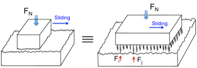
Figure 1: Contact of two surfaces, one of the surfaces is approximated by a set of discrete elements, the other surface is assumed to be rigid. The only degree of freedom of the elements is normal to the interface.

2.1 Setting

The contact between two rough surfaces is dominated by the interaction between a small number of asperities on the two surfaces. We model one of these surfaces as a collection of a regular array of discrete deformable elements attached to a rigid block while we model the other as a rigid rough surface (Figure 1). Contact is determined by the interaction between a small number of discrete elements with peaks on the rigid surface, thereby mimicking the interaction between asperities. We denote the relaxed (or stress-free) length of the $i^{\text{th}}$ element by $z_{i}^{0}$ and its reference lateral position by $(x_{i}^{0},y_{i}^{0})$. The height of the rough surface at the position $(x,y)$ is $h(x,y)$.

The kinematic state of the system is described by two macroscopic variables – the dilatation or nominal separation $d$ between the two surfaces and the relative lateral distance $\bar{x}$ of one surface relative to the other (or equivalently the distance of sliding) – and $N$ microscopic variables $u_{i}$ describing the change in lengths of the elements from its original length (so that the total length of the element is $z_{i}^{0}+u_{i}$). At any given dilatation $d$ and lateral position $\bar{x}$, the distance between the $i^{\text{th}}$ element and the rough surface is

$$d_{i}=d-z_{i}^{0}-u_{i}-h(x_{i}^{0}+\bar{x},y_{i}^{0}).$$ (4)

We require $d_{i}\geq 0$ to represent the non-interpenetrability of matter. Further, $d_{i}=0$ signifies the contact of the $i^{\text{th}}$ element with the rough surface.

Corresponding to the kinematic variables, we have two macroscopic forces – the macroscopic normal force $F_{N}$ and the macroscopic shear force $F_{S}$ – as well as $N$ microscopic normal forces $F_{i}$ and $N$ microscopic shear strengths $S_{i}$. In this work, we assume that adhesion is negligible and hence the force on the $i^{\text{th}}$ element is always compressive: $F_{i}\leq 0$.

We postulate time-dependent constitutive relations at the microscopic scale – one between the length change $u_{i}$ and force $F_{i}$ of each element, and another for the microscopic strength $S_{i}$. We then study the equilibrium of the system ($F_{N}=\sum F_{i}$, $F_{S}=\sum S_{i}$) to infer the macroscopic contact and friction laws.

2.2 Rough surface

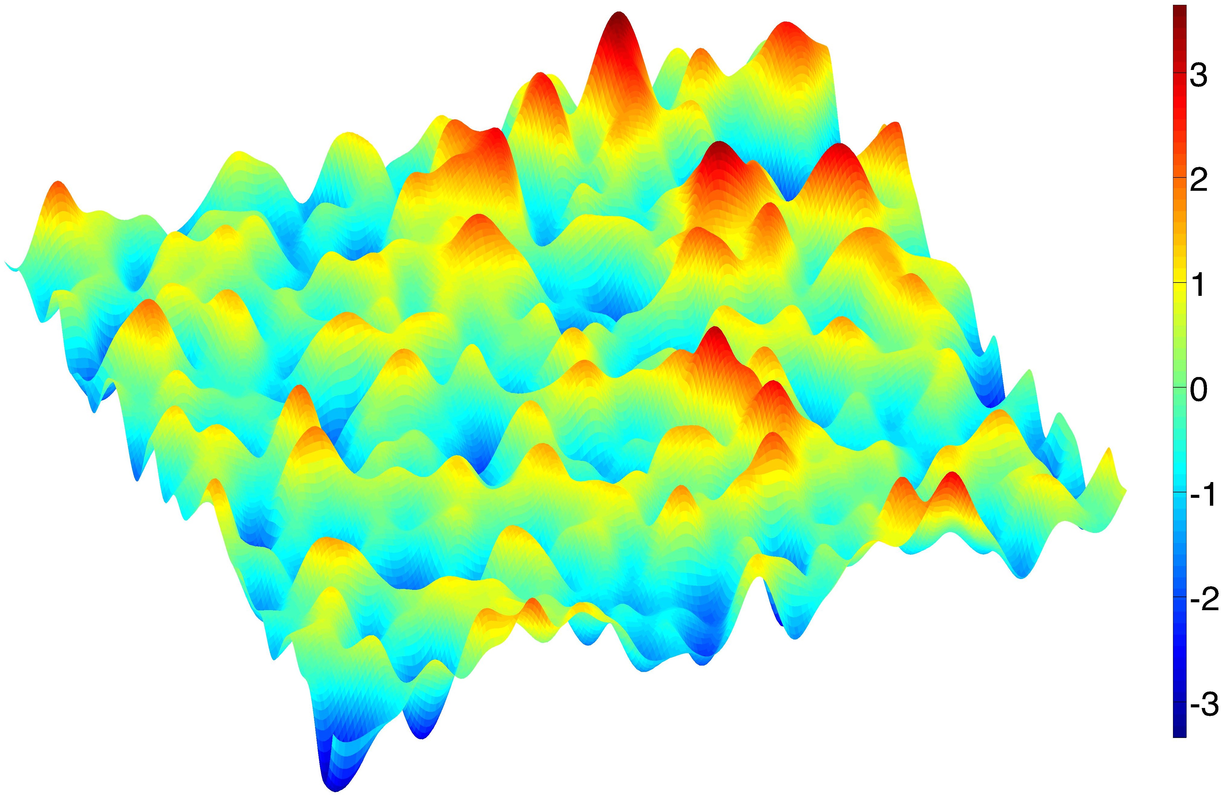
(a)

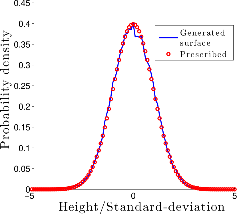
(b)

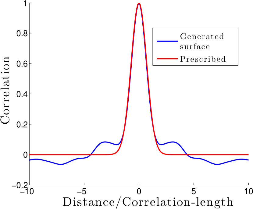
(c)

Figure 2: (a) Rough surface with a Gaussian distribution of heights and a Gaussian autocorrelation (vertical features magnified). Statistical properties of the generated surfaces: (b) probability density (Gaussian) of heights, and (c) Gaussian spatial correlation.

Rough surfaces have been characterized as a stochastic process [33, 34, 35] and this characterization has been used extensively in exploring various aspects of contact between surfaces [31, 36, 37]. The stochastic process is specified by two functions, a probability distribution of heights which describes features normal to the interface and an autocorrelation function which is related to how the vertical features vary along the interface. For many surfaces, the probability distribution of heights is Gaussian,

$$P(h)=\frac{1}{\sigma\sqrt{2\pi}}e^{-h^{2}/(2\sigma^{2})},$$

where $h$ is the height of a surface from the mean, $P(h)$ is the probability density, and $\sigma$ is the root mean square roughness [38]. The autocorrelation is found to decay exponentially or as a Gaussian [38, 39]. In this study, we consider surfaces with a Gaussian autocorrelation:

$$R(\delta_{x},\delta_{y})=\langle h(x,y)h(x+\delta_{x},y+\delta_{y})\rangle=\sigma^{2}e^{-(\delta_{x}^{2}/\beta_{x}^{2}+\delta_{y}^{2}/\beta_{y}^{2})},$$

where $R$ is the autocorrelation function, $\beta_{x},\beta_{y}$ are the correlation lengths along $x$ and $y$ directions, and $\langle\ \rangle$ denotes expectation with respect to the probability distribution.

Rough surfaces with these statistical properties are created by generating a set of independent Gaussian random numbers and using a linear filter [40]. The weights of the linear filter are determined from the autocorrelation. The heights of the resulting rough surfaces are known only at discrete locations and are interpolated using a cubic spline for intermediate values. A typical realization of such a surface, its probability distribution of heights and autocorrelation are shown in Figure 2. The generated surface shows a good match with the prescribed properties.

Since we are interested in two rough surfaces, we need to use two stochastic processes, one for the rigid rough surface $h(x,y)$ and one for the elements $z_{i}^{0}$. However, in this work, we take all the elements to have the same stress-free heights $z_{i}^{0}=0$. We can see from (4) that this does not pose a loss of generality when we are in static contact ($\bar{x}=0$) since we may redefine $z_{i}^{0}+h(x_{i},y_{i})$ to be a random variable as long as we understand the statistics to be the joint statistics of the two surfaces. However, this is a non-trivial assumption in the case of sliding contact, especially in the case of viscoplastic interactions.

In what follows, we non-dimensionalize the equations. In part, we introduce a characteristic length $L^{*}$ and set $\bar{h}=h/L^{*},\bar{\sigma}=\sigma/L^{*},$ etc. Since the characteristic root-mean-square roughness ($\sigma$) of most experimental surfaces is of the order of 1 $\mu$m [38], we take $L^{*}=1\ \mu$m.

2.3 Constitutive relation for the deformation of the elements

In this work, we consider three different kinds of constitutive relations for the deformation of the elements. The first two are viscoelastic and the third is viscoplastic. We note that, in the viscoelastic models, the change in length $u_{i}$ eventually (exponentially in time) returns to zero when the force is released.

2.3.1 Viscoelastic element without elastic interactions

Here we assume that the length change $u_{i}$ of element $i$ depends only on its force history and is governed by a finite number $N_{T}$ of relaxation times. Therefore, given a force history $F_{i}(t)\leq 0$,

$$u_{i}(t) =C^{0}\left[F_{i}(t)+\int_{0}^{t}\sum_{k=1}^{N_{T}}A_{k}e^{-\lambda_{k}(t-\tau)}F_{i}(\tau)\ \mathrm{d}\tau\right]$$ (5)

where $C^{0}$ is the elastic compliance of the elements and $A_{k}$ is the amplitude of the viscoelastic effect associated with the $k^{\text{th}}$ relaxation rate $\lambda_{k}$. Most of our examples use a single relaxation rate ($N_{T}=1$).

It is convenient to non-dimensionalize the equations. We use $L^{*},T^{*},F^{*}$ to nondimensionalize length, time and force and set

$$\bar{u}=\frac{u}{L^{*}},\quad\bar{t}=\frac{t}{T^{*}},\quad\bar{\tau}=\frac{\tau}{T^{*}},\quad\bar{F}=\frac{F}{F^{*}},\quad\bar{A}_{k}=A_{k}T^{*},\quad\bar{\lambda}_{k}=\lambda_{k}T^{*},\quad\bar{C}^{0}=\frac{C^{0}F^{*}}{L^{*}},\quad\dots$$ (6)

Substituting these into (5), the equation remains unchanged except all terms are non-dimensional (replace unbarred symbols with barred ones).

To understand this constitutive equation, assume that we have a single relaxation rate $\bar{\lambda}$. Consider a force $\bar{F}_{j}(\bar{t})=\bar{F}^{0}_{j}H(\bar{t})$, where $H(\bar{t})$ is the Heaviside function. For $\bar{t}>0$,

$$\bar{u}_{i}(\bar{t})=\bar{C}_{0}\left[1+\frac{\bar{A}}{\bar{\lambda}}\left(1-e^{-\bar{\lambda}\bar{t}}\right)\right]\bar{F}^{0}_{j}.$$

If $\bar{t}\ll 1/\bar{\lambda}$,

$$\bar{u}_{i}(\bar{t})\approx\bar{C}_{0}\bar{F}^{0}_{j},$$

and for $\bar{t}\gg 1/\bar{\lambda}$,

$$\bar{u}_{i}(\bar{t})\approx\bar{C}_{0}(1+\bar{A}/\bar{\lambda})\bar{F}^{0}_{j}.$$

Thus, the instantaneous compliance of the system is $\bar{C}_{0}$, the steady-state compliance is $(1+\bar{A}/\bar{\lambda})\bar{C}_{0}$, and the length change reaches steady state at the decay rate $\bar{\lambda}$.

Since the typical timescale of static friction growth in rocks is of the order of seconds [6], we take $T^{*}=1$ sec. As before, we take $L^{*}=1\ \mu$m.

2.3.2 Viscoelastic element with Boussinesq interaction

Here, the length change $u_{i}$ of element $i$ depends not only on force history of that element, but also on the force history of all the other elements. As before, we assume that the viscoelastic response is governed by a finite number $N_{T}$ of relaxation times. However, the interaction between elements $i$ and $j$, for $i\neq j$, depends on the distance $r_{ij}$ between the elements. Specifically, we assume that given a force history $F_{i}(t)\leq 0$,

$$\begin{split}u_{i}(t)&=\frac{1-\nu}{2\pi G}\left[\frac{3.8}{\Delta}\left(F_{i}(t)+\int_{0}^{t}\sum_{k=1}^{N_{T}}A_{k}e^{-\lambda_{k}(t-\tau)}F_{i}(\tau)\mathrm{d}\tau\right)\right.\\ &\phantom{asdfasdfasdf}+\left.\sum_{j\neq i}\frac{1}{r_{ij}}\left(F_{j}(t)+\int_{0}^{t}\sum_{k=1}^{N_{T}}A_{k}e^{-\lambda_{k}(t-\tau)}F_{j}(\tau)\mathrm{d}\tau\right)\right].\end{split}$$ (7)

where $G$ is the shear modulus and $\nu$ the Poisson’s ratio of the medium, $\Delta$ is the distance between neighboring elements and $A_{k}$ is the amplitude of the viscoelastic effect associated with the $k^{\text{th}}$ relaxation rate $\lambda_{k}$. Most of our examples use a single relaxation rate.

The constitutive relation above is motivated by the Boussinesq solution that describes the normal displacement $u(r)$ at position $r$ on the surface of a homogeneous elastic half-space due to an applied normal force $F$ at the origin (e.g. [41]):

$$u(r)=\frac{1-\nu}{2\pi G}\frac{F}{r}.$$

This equation, the superposition principle and the viscoelastic correspondence principle motivate the form of (7) when $i\neq j$. Note that the expression becomes singular when $i=j$ since $r=0$. However, this singularity is regularized if the point force is replaced by a uniform pressure over an area. Therefore we assume that $F_{i}$ is uniformly distributed over a square area of side-length $\Delta$ (the distance between the elements). The first term (with the factor 3.8) is obtained using a solution by Love [42] and the viscoelastic correspondence principle.

We non-dimensionalize the equations according to (6) and $\bar{r}_{ij}=r_{ij}/L^{*},\bar{\Delta}=\Delta/L^{*}$. As mentioned before, we take $L^{*}=1\ \mu$m. We assume $T^{*}=1$ s and set $F^{*}=\frac{2\pi G{L^{*}}^{2}}{1-\nu}$ so that our constitutive relation is

$$\begin{split}\bar{u}_{i}(t)&=\frac{3.8}{\bar{\Delta}}\left(\bar{F}_{i}(\bar{t})+\int_{0}^{\bar{t}}\sum_{k=1}^{N_{T}}\bar{A}_{k}e^{-\bar{\lambda}_{k}(\bar{t}-\bar{\tau})}\bar{F}_{i}(\bar{\tau})\mathrm{d}\bar{\tau}\right)\\ &\phantom{asdfasdfasdf}+\sum_{j\neq i}\frac{1}{\bar{r}_{ij}}\left(\bar{F}_{j}(\bar{t})+\int_{0}^{\bar{t}}\sum_{k=1}^{N_{T}}\bar{A}_{k}e^{-\bar{\lambda}_{k}(\bar{t}-\bar{\tau})}\bar{F}_{j}(\bar{\tau})\mathrm{d}\bar{\tau}\right).\end{split}$$ (8)

By considering a situation with one relaxation time and applying a step load, we can see that the instantaneous and steady-state compliance of the system are $3.8/\bar{\Delta}$ and $3.8(1+\bar{A}/\bar{\lambda})/\bar{\Delta}$ respectively when $i=j$ and $1/\bar{r}_{ij}$ and $(1+\bar{A}/\bar{\lambda})/\bar{r}_{ij}$ respectively when $i\neq j$.

2.3.3 Elastic/viscoplastic element

Here we assume that the element can undergo permanent deformation through viscoplastic creep. We specify this constitutive relation directly in non-dimensional quantities. First, the total length change is split into elastic (recoverable) and plastic (permanent) parts:

$$\bar{u}_{i}=\bar{u}_{i}^{e}+\bar{u}_{i}^{p}$$ (9)

where $\bar{u}_{i},\bar{u}_{i}^{e},\bar{u}_{i}^{p}$ are the total, elastic, and plastic length changes, respectively, of the $i^{\text{th}}$ element.

The elastic length change is linearly related to the force, and we take this to be nonlocal:

$$\bar{u}_{i}^{e}=\sum_{i,j}\bar{C}_{ij}\bar{F}_{j}$$ (10)

where $\bar{C}_{ij}$ is the compliance and it is taken to be the elastic part of (8).

The evolution of the plastic deformation is local, and it is given by a power-law creep where the rate of change of the plastic length change depends on the current force and the history of the plastic deformation

$$\dot{\bar{u}}_{i}^{p}=\bar{A}_{cr}(|\bar{F}_{i}|/{\bar{F}}_{i}^{y})^{n}\text{ sign}(\bar{F}_{i}),$$ (11)

where ${\bar{F}}_{i}^{y},\bar{A}_{cr},n$ are the yield force, the creep rate, and the creep exponent, respectively. $\bar{A}_{cr}$ and $n$ are material constants. The yield force $\bar{F}_{i}^{y}$ of the $i^{\text{th}}$ element evolves with the deformation according to the following hardening law:

$$\dot{{\bar{u}}}_{i}^{acc}=|\dot{{\bar{u}}}^{p}|,{\bar{F}}_{i}^{y}={\bar{F}}_{y}^{0}(1+\bar{B}{\bar{u}}_{i}^{acc})^{m},$$ (12)

where ${\bar{u}}_{i}^{acc},{\bar{F}}_{y}^{0},\bar{B},m$ are the accumulated plastic length change in the $i^{\text{th}}$ element, the initial yield stress, the hardening rate and the hardening exponent, respectively. The last three are material parameters.

2.4 Calculation of macroscopic friction coefficient

The friction coefficient is given by the ratio of the macroscopic shear strength $\bar{F}_{S}$ to the normal force $\bar{F}_{N}$:

$$\mu=\frac{\bar{F}_{S}}{\bar{F}_{N}},$$ (13)

where $\bar{F}_{S}=\sum_{i}\bar{S}_{i}$ and $\bar{S}_{i}$ is the shear force on element $i$. We assume that the shear force that any element in contact with the rough surface can sustain depends on the shear strength of the material. Therefore, for an element in contact,

$$\bar{S}_{i}=\begin{cases}\bar{\tau}_{S}\bar{A}_{i}&\bar{v}=0\\ \displaystyle{\left(\bar{\tau}_{S}+\alpha\log(\bar{v})\right)\bar{A}_{i}}&\text{else}\\ \end{cases}$$ (14)

where $\bar{\tau}_{S}$ is the (non-dimensional) shear strength of the material, $\bar{A}_{i}$ is area of element $i$, $\alpha$ is the velocity-hardening coefficient, and $\bar{v}$ is the sliding velocity. Importantly, we assume that the microscopic shear force is independent of the microscopic normal force as long as the element is in contact. If the surfaces are in static contact, the shear strength is $\bar{\tau}_{S}$. If the surfaces are sliding at a relative speed $\bar{v}$, the asperities in contact are sheared at a strain rate proportional to the sliding speed, and if the shear resistance depends on the strain rate, then the local friction law will be velocity-dependent. Taking cue from experimental results, we assume this velocity dependence to be logarithmic. A theoretical justification for the logarithmic dependence has been proposed by Rice et al. [43].

Summing equation (14) over all elements in contact,

$$\bar{F}_{S}=\begin{cases}\bar{\tau}_{S}\bar{A}&\bar{v}=0,\\ \displaystyle{\left(\bar{\tau}_{S}+\alpha\log(\bar{v})\right)\bar{A}}&\text{else,}\\ \end{cases}$$ (15)

where the total contact area $\bar{A}$ is given by the sum of all elements in contact.

2.5 Simulation of evolving contacts

Now that we have the rough surfaces and the constitutive equations for the elements, let us look at the simulation of static/sliding contact. Consider two rough surfaces in contact under a given macroscopic normal force $\bar{F}_{N}$ and sliding at a velocity $v$ relative to each other ($v=0$ for static contact). We seek to use the model above to determine the time-evolution of the macroscopic shear force $\bar{F}_{S}$ and the macroscopic dilatation $\bar{d}$. We are also interested in the statistical features of the contact.

We assume that we know the prior history of all microscopic variables up to some time which we set as $\bar{t}=0$. We now solve for the microscopic variables $\bar{u}_{i}(\bar{t}),\bar{F}_{i}(\bar{t})$ and the macroscopic variable $\bar{d}(\bar{t})$ satisfying the appropriate constitutive relation (CR) in Section 2.3 subject to the constraints

$$\bar{d}_{i}(\bar{t})\bar{F}_{i}(\bar{t})=0,\quad\bar{d}_{i}(\bar{t})\geq 0,\quad\bar{F}_{i}(\bar{t})\leq 0;$$ (16)

$$\bar{F}_{N}(\bar{t})=\sum_{i}\bar{F}_{i}(\bar{t})$$ (17)

where $d_{i}$ is given by (4) with $\bar{x}(t)=\bar{v}\bar{t}$.

We implement the model numerically by discretizing the constitutive relations using a first-order Euler method and applying an iterative approach as described in detail in Algorithm 1. Note that (CR) refers to the appropriate constitutive relation of the element.

Given $\bar{F}_{N},\bar{v}$, constitutive relation for each element denoted by (CR) below

Given history $\bar{u}_{i}(\bar{\tau}),\bar{F}_{i}(\bar{\tau}),\bar{d}(\bar{\tau})$ for $\bar{\tau}\leq\bar{t}$

repeat Take a time step $\bar{t}\to\bar{t}+\Delta\bar{t}$

       Assume the set of elements in contact $\mathcal{I}_{c}$ does not change in the time-step $\Delta\bar{t}$.

       Guess two dilatation rates $\dot{\bar{d_{1}}}$ and $\dot{\bar{d_{2}}}$. One of these can be dilatation rate of the previous time-step. Compute two dilatation guesses $\bar{d}_{1}(\bar{t}+\Delta\bar{t})$ and $\bar{d}_{2}(\bar{t}+\Delta\bar{t})$. We will use a secant root-finding method to find the new dilatation that conserves the total normal force.

       repeat

             For each rate

             for $i=1,\dots,N$ do

                   if $i\in\mathcal{I}_{c}$ then

                        set $\bar{d}_{i}(\bar{\tau})=0$ for $\bar{\tau}\in(\bar{t},\bar{t}+\Delta\bar{t})$ and use (CR) to compute $\bar{F}_{i}(\bar{t}+\Delta\bar{t})$

                  else

                         set $\bar{F}_{i}(\bar{\tau})=0$ for $\bar{\tau}\in(\bar{t},\bar{t}+\Delta\bar{t})$ and use (CR) to compute $\bar{u}_{i}(\bar{t}+\Delta\bar{t})$

                  

            Compute the total force $\sum_{i}\bar{F}_{i}(\bar{t}+\Delta\bar{t})$ at the two rates. Call these $\bar{F}_{N}^{1},\bar{F}_{N}^{2}$.

             Use the secant root-finding method with the new dilatation rate guess $\dot{\bar{d}}_{\text{new}}=\dot{\bar{d_{1}}}+(\dot{\bar{d_{2}}}-\dot{\bar{d_{1}}})(\bar{F}_{N}-\bar{F}_{N}^{1})/(\bar{F}_{N}^{2}-\bar{F}_{N}^{1})$

      until $\sum\bar{F}_{i}(\bar{t}+\Delta\bar{t})=\bar{F}_{N}$;

      Use (15) to compute $\bar{F}_{S}(\bar{t}+\Delta\bar{t})=\sum S_{i}(\bar{t}+\Delta\bar{t}),\ i=1,\dots,N$

       for $i=1,\dots,N$ do

             if $\bar{F}_{i}>0$ then

                  set $\bar{F}_{i}=0$, remove $i$ from $\mathcal{I}_{c}$ (loss of contact)

            if $\bar{d}_{i}<0$ then

                  set $\bar{d}_{i}=0$, add $i$ from $\mathcal{I}_{c}$ (contact formed)

            

       Note $I_{c},\{u_{i}\},\{\bar{F}_{i}\},\bar{d},$ at $\bar{t}+\Delta\bar{t}$

       Compute $\mu(\bar{t}+\Delta\bar{t})$ from (13)

      

until $\bar{t}=\bar{T}$;

Algorithm 1 Algorithm to simulate contact under a given global normal force.

2.5.1 Computational memory and complexity considerations

In the Boussinesq interaction case, because the deformation due to a point force decays only as $1/r$, the compliance matrix $C_{ij}$ is dense and for a large system, storing the matrix entries leads to large memory requirements. We circumvent this challenge by computing the matrix-vector product $C_{ij}F_{j}$ in a matrix-free way and using an iterative solver (GMRES) [44] when a linear system needs to be solved. Because of the $1/r$ decay, a brute force computation of the interactions would involve $O(N^{2})$ operations where $N$ is the number of elements, and this can be prohibitively expensive for large systems. Two things come to our rescue here. First, for rough surfaces, the actual area of contact is only a small fraction of the nominal area; so, at any instant of time, the forces are nonzero for only a small fraction of the elements and only these elements need to be considered in computing the displacements. Second, the $1/r$ interactions can be computed to within prescribed error tolerance in $O(N\log(N))$ operations using the Fast Multipole Method (FMM) [45, 46]. In all results presented here, we use an FMM method of order $5$ since which we found to be sufficient by comparison with a brute force calculation.

2.6 Parameters used in simulations

Unless mentioned otherwise, the parameters used in our simulations are listed in Table 1.

Parameter	Value
System size	512 $\mu$m by 512 $\mu$m
No-interaction elastic compliance $\bar{C}^{0}$	16 (Section 2.3.1)
Shear modulus $G$	30 GPa
Poisson ratio $\nu$	0.25
Rough surfaces	Flat deformable against rough rigid
Probability distribution of heights	Gaussian
Rms-roughness $\sigma$	1 $\mu$m
Autocorrelation of heights	Gaussian
Correlation lengths $\beta_{x},\beta_{y}$	10 $\mu$m
Viscoelasticity parameters	$\bar{\lambda}=1,\bar{A}=0.2$
Viscoplasticity parameters	$n=3,\bar{A}_{cr}=10^{-4}$ $\bar{F}_{y}^{0}=0.016,\bar{B}=0,m=1$ (Section 2.3.3)
Static shear strength $\tau_{S}$	2.5 GPa (Equation 14)
Velocity-hardening parameter $\alpha$	0.0002 (Equation 14)

Table 1: Parameters used in our simulations.

$G,\nu$ values are typical for rocks. The shear strength $\tau_{S}$ of a contact can be a significant fraction of the shear modulus [43, 47], here we use $\tau_{S}$ = 2.5 GPa. $\bar{F}_{y}^{0}=0.016$ corresponds to a yields stress of 4 GPa. We choose $\bar{C}^{0}=16$ since this gives us true contact areas of the order of 1% of nominal areas, similar to experimental observations.

The main parameters that vary in the following simulations are the material behavior (viscoelastic parameters $\bar{\lambda},\bar{A}$ and the viscoplasticity parameters in Table 1), the constitutive response (with or without long-range elastic interactions), and the sliding velocity $\bar{v}$. All our simulations use the same rough surface.

3 Validation using Hertzian contact

To validate our formulation, we simulate the Hertzian contact of a homogenous linear-elastic sphere of radius $1$ with a rigid flat surface. The geometry of the sphere is simulated using the undeformed lengths of the elements. The two surfaces are initially apart, and the force and length changes of all the elements are initialized to zero. The surfaces are then brought into contact by decreasing the dilatation. The evolution of the length changes and forces of the elements is computed using an algorithm similar to Algorithm 1 but with the dilatation prescribed.

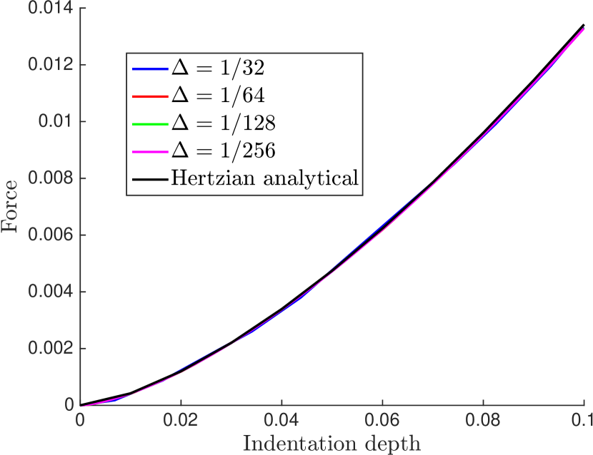
(a)

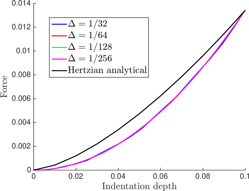
(b)

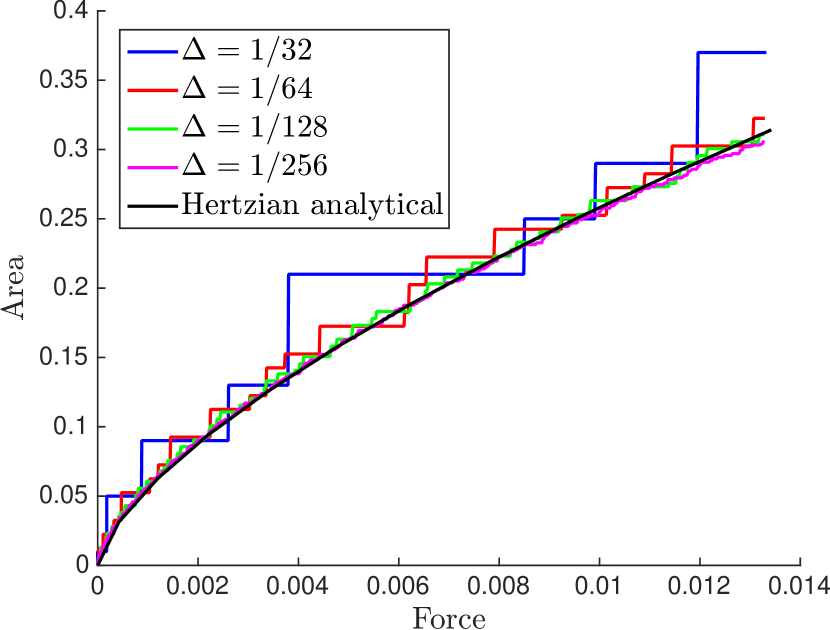
(c)

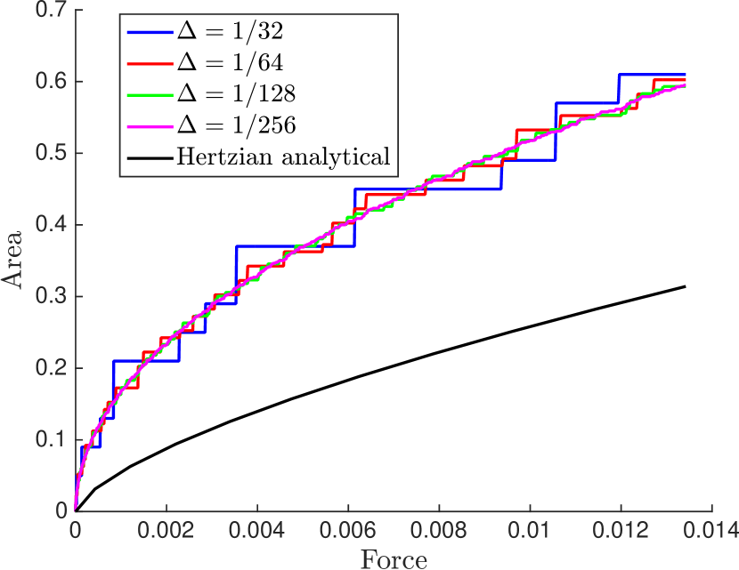
(d)

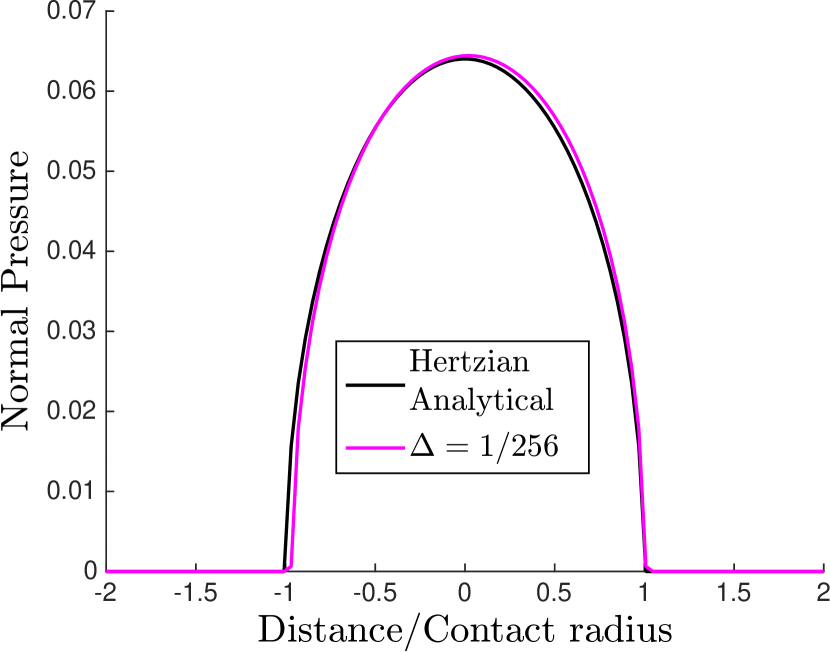
(e)

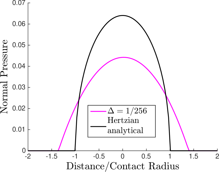
(f)

Figure 3: Comparison of analytical and numerical solutions for contact of a linear-elastic sphere against a rigid flat: (left column) with Boussinesq interaction, (right column) with no elastic interaction. Lines of different colors correspond to different discretization sizes $\Delta$, the distance between the elements.

In the case with Boussinesq interaction, there is an excellent match between the numerical and analytical solutions (Figure 3). The elastic constants used in the analytical and numerical solutions are the same and no other parameters are used in obtaining the numerical results. For the case with no elastic interaction, $\bar{C}^{0}$ is chosen to make the force at the final indentation match the analytical solution. However, we find that the scaling of the force and area deviates from the Hertzian solution in this case.

4 Static contact

We start by considering the static contact of rough surfaces. The surfaces, initially apart, are loaded “instantaneously” to a nominal pressure of $100$ MPa. The system is then evolved keeping the global normal force constant. The evolution of the forces, length changes of the elements, and contact area is computed. Let us first look at the viscoelastic case.

4.1 Evolution of contact and force distribution

After the initial compression, the forces at the contacts start relaxing because of the viscoelastic behavior. To keep the global normal force constant, more contacts are formed and the contact area increases. As in experiments [7], existing contacts grow with time, some contacts coalesce, and some new ones are formed (Figure 4).

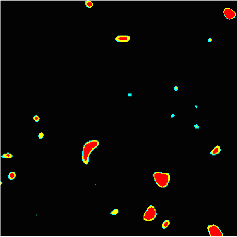
(a)

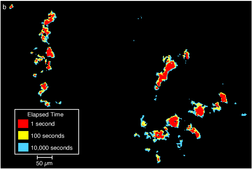
(b)

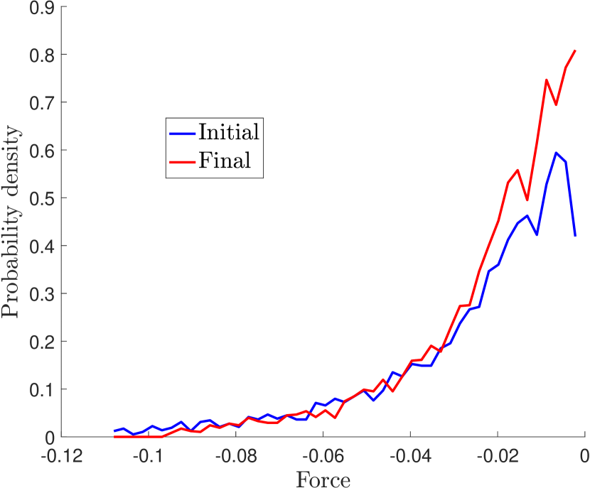
(c)

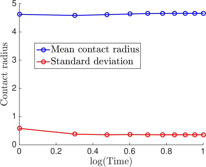
(d)

Figure 4: Evolution of contacts, in (a) our simulations and (b) experiments [7], during a static contact test. In (a), contacts at $\bar{t}=0$ are in red, $\bar{t}=10$ are in yellow, and $\bar{t}=100$ are in cyan. Existing contacts grow, some coalesce, and some new contacts are formed. Panel (b) is reproduced with permission from [7]. (c) Distribution of contact forces at the initial and final states. Initially, the area of contact is lower but the average force on a contact is higher. With time, as the forces relax, the number of contacts increases but the average force per contact decreases. (d) Evolution of the average contact size with time (the mean and standard deviation are computed across $15$ realizations of the rough surface). Even though the total contact area increases, the average contact size does not change significantly.

As contact forces relax and contact area increases, the force distribution spreads and the force per unit contact area decreases (Figure 4(c)). The first moment of the force distribution, which is the total normal force, is the same for initial and final states, by the design of the numerical experiment. The zeroth moment (area under the curve), which is the total contact area, is larger at the final state.

Even though the total contact area increases, the average contact radius, calculated as $\sqrt{\text{Contact area}/(\pi\times\text{Number of contacts})}$, remains nearly constant (Figure 4(d)). This is because, as the contact area increases, the number of contacts also increases keeping the average contact radius approximately constant. A similar observation was made by Greenwood and Williamson in their statistical model of elastic contacts [31] and in experiments [7].

4.2 Increase of contact area and friction with time

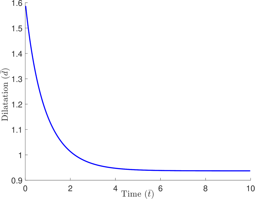
(a)

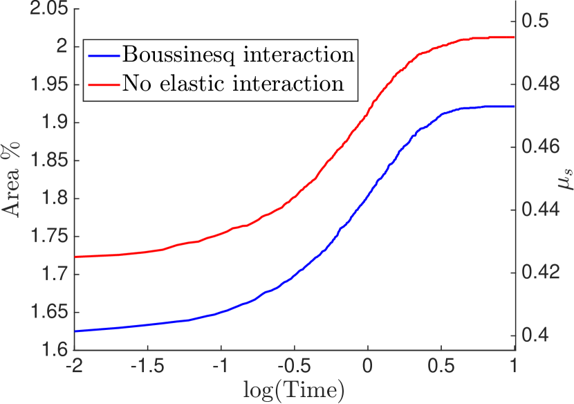
(b)

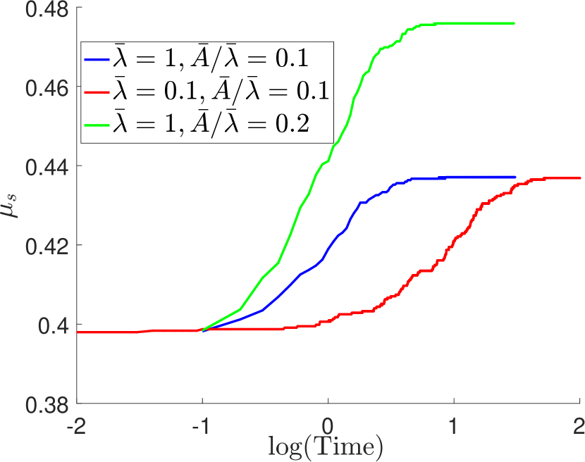
(c)

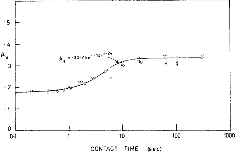
(d)

Figure 5: Evolution of (a) dilatation and (b) contact-area/friction-coefficient with the time of contact. Because of viscoelastic relaxation, the surfaces move closer and the area of contact increases with time. The timescale and the magnitude of evolution are unchanged by the presence of long-range Boussinesq interactions. (c) Evolution of friction coefficient for three different combinations of viscoelastic parameters. The timescale of evolution is determined by $\bar{\lambda}$ and the difference between initial and final states is determined by the ratio $\bar{A}/\bar{\lambda}$. For some duration, the growth is logarithmic in time and saturates to a steady state at long times. (d) Evolution of friction coefficient in experiments of Richardson et al. (reproduced with permission from [48]) showing similar behavior.

As the individual contact forces relax, dilatation decreases (the surfaces move closer to each other) and the contact area increases (Figure 5(a)). Consequently, the static friction coefficient always increases with time (Figure 5(b)) and this has been universally observed in experiments [4, 5, 48]. In Figure 5(b), there is a logarithmic growth phase that lasts about $3$ decades in time. If we have only one relaxation time, then saturation time is inversely proportional to $\lambda$ as can be seen by from the constitutive equations (5) and (7). If $\{u(t,\lambda),F(t,\lambda)\}$ is a solution, then so is $\{u(nt,\lambda/n),F(nt,\lambda/n)\}$. In some materials like mild steel, a similar duration of static friction growth with saturation at small and long times is observed [48], as shown in Figure 5(d). Thus, our results are consistent with these experimental observations.

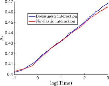
Figure 6: Evolution of friction coefficient during static contact for a material with four viscoelastic timescales. The region of logarithmic growth lasts over $4$ decades, as seen in experiments on rocks.

In experiments on rocks, the logarithmic growth persists throughout the duration of the experiments, some of which have lasted up to six decades in time [5, 6]. We find that there are two possible reasons.

Multiple relaxation times lead to an extended period of increase.

The simulations above considered a constitutive relation with a single relaxation time. However, common materials have multiple relaxation times. Longer timescales of relaxation lead to longer times of growth in contact area and hence friction. To study the dependence of friction evolution of the viscoelastic properties, we perform static contact simulations for three different combinations of the parameters $\bar{\lambda}$ and $\bar{A}$ (Figure 5(c)). The blue and green curves (both have $\bar{\lambda}=1$) reach steady state at about the same time but the magnitude of the change in friction is different. The blue and red curves have different $\bar{\lambda}$ and thus reach steady state at different times. However, they have the same $\bar{A}/\bar{\lambda}$ and thus the steady-state friction coefficient is the same. This tells us that the timescale of evolution of area and friction is determined by $\bar{\lambda}$ while the steady state stiffness (and the magnitude of the difference between the initial and final states) is determined by the ratio $\bar{A}/\bar{\lambda}$. The initial value of friction is determined by the instantaneous stiffness of the system (stiffness corresponding to fast loading rates) and is hence independent of the viscoelastic properties. If we thus have a material with multiple relaxation times, the growth in friction will persist over times corresponding to the longest relaxation time. This is confirmed in Figure 6 where the material has four viscoelastic relaxation timescales ($N_{T}=4,\bar{\lambda}_{k}=1,0.1,0.01,0.001,\bar{A}_{k}=0.05,0.005,0.0005,0.00005$). The linear growth regime of friction now extends over four decades in time.

Viscoplasticity also leads to continued increase.

We now repeat the simulations assuming the viscoplastic constitutive relation (Section 2.3.3). As in the viscoelastic case, the area of contact and thus $\mu_{s}$ increase with the time of contact and, after an initial phase, grows logarithmically with time (Figure 7). In the viscoelastic case, the growth saturates after about $3$ decades. However, here the growth seems to continue indefinitely and shows no signs of saturation. This is expected from the viscoplastic model without hardening, since the contacts continue to creep under any nonzero force. Figure 7 also shows the dependence of the friction evolution on the creep rate $\bar{A}_{cr}$. Larger creep rates lead to a faster and larger growth in $\mu_{s}$ (also see [25]).

Elastic interactions do not change qualitative behavior.

We find that that static friction evolution with and without long-range elastic interactions is qualitatively the same (Figures 5(b) and 6). The elastic interactions do not affect either the duration or the magnitude of friction growth.

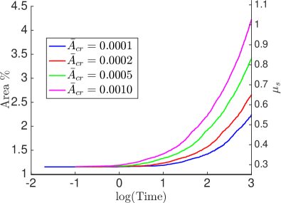
Figure 7: Evolution of contact area and static friction coefficient with time for a viscoplastic material. $\mu_{s}$ grows logarithmically with time with no signs of saturation, as seen in many experiments.

4.3 Friction coefficient is nearly independent of the normal force

The friction coefficient is known to be independent of the normal force for macroscopic rough surfaces (Amontons law). In the Bowden and Tabor model, this is explained by the plasticity of contacts [3], whereas in the Greenwood-Williamson (GW) model, this is a result of the statistics of the rough surface [31]. The GW model ignores interactions between contacts which might be important. Our simulations suggest that both with and without elastic interactions, the friction coefficient is nearly independent of the applied normal pressure (Figure 8).

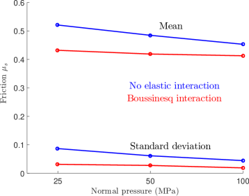
Figure 8: Dependence of friction coefficient on normal pressure for three system sizes. The mean and the standard deviation for $15$ realizations is shown. Considering the mean and the standard deviation, the friction coefficient is independent of both the system size and the applied nominal pressure.

5 Sliding contact

Let us move on to the sliding contact of rough surfaces. The results presented here are for a $512\times 512$ deformable rough surface sliding on a larger $512\times 1024$ rigid flat surface. We conduct two kinds of numerical experiments. First, to study sliding at a given sustained velocity $\bar{v}$, we compress two rough surfaces to a nominal pressure of $100$ MPa and, starting at the same initial state, slide at $\bar{v}$ until the contact area and macroscopic friction reach steady state (sections 5.1-5.3). Note that the correlation length for our rough surface is of the order of 10, and thus we achieve steady state when we slide over distances of a few times the correlation length. Then, we conduct velocity jump experiments (sections 5.4-5.6).

5.1 Evolution of contacts

As a deformable element slides on the rigid rough surface, its length and normal force evolve depending on the surface profile it encounters, as well on the long-range interactions with other elements. The evolution of a typical element during sliding is shown in Figure 9. The element repeatedly comes into and goes out of contact with the surface. When not in contact, its normal force is zero, and the change in its length depends on its viscoelastic relaxation as well as on the evolution of the global dilatation of the surface, to keep the global normal force constant. For example, the wiggles of the element height in the region marked as $1$ are from the variations in the global dilatation (to keep the normal force constant). In the region marked $2$, the element height rapidly increases, because of a rapid change in the global dilatation.

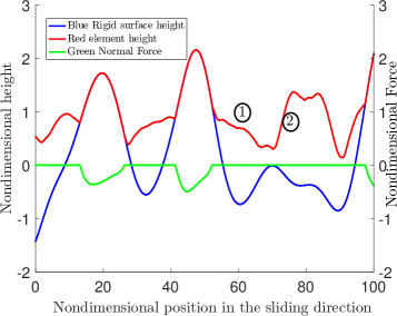
Figure 9: Evolution of a single element as it slides along a rough surface in a simulation with viscoelastic properties and long-range interactions. The element is initially out of contact and the force is zero. As it slides, it repeatedly comes into and goes out of contact with the rigid surface and correspondingly, the force on it also evolves. The element also gets perturbed by the overall dilatation of the sliding surface.

As the deformable surface slides on the rigid rough one, the elements and their forces evolve as an ensemble (Figure 10). Contacts form, some of them grow, while others dwindle. With continuing slip, eventually all of them go out of existence, replaced by others.

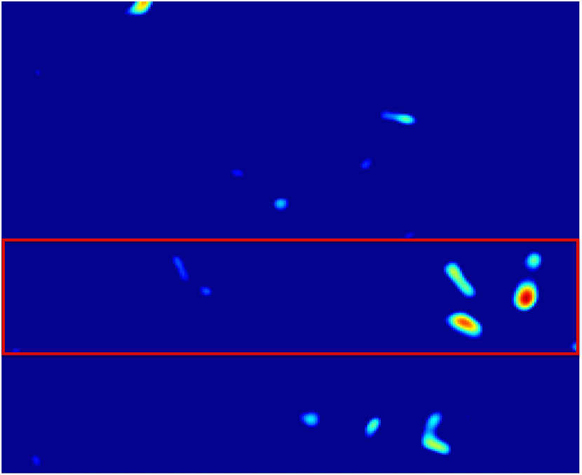
(a)

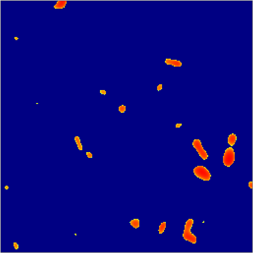
(b)

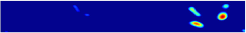
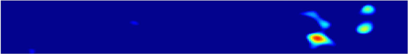
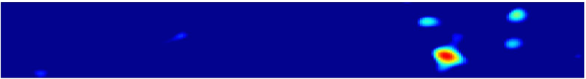
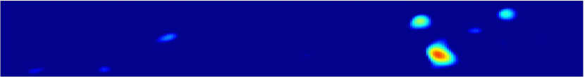
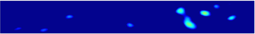
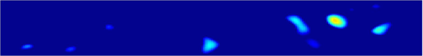
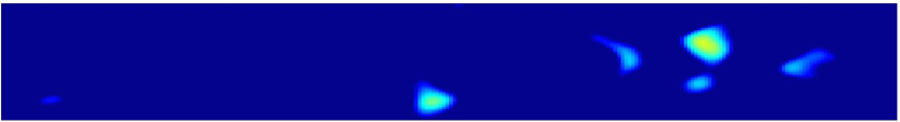
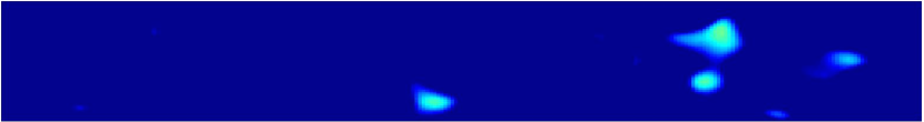
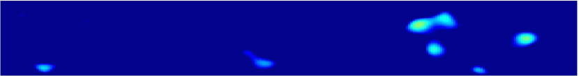
(c)

Figure 10: Evolution of forces on a subset of the elements of the surface during sliding. The subset of elements considered in (c) is marked by a red box in (a). (b) shows the forces in (a) on a logarithmic scale (to better display the smaller forces not evident in (a)). The color in (a) and (c) indicates the nondimensionalized normal force on each element. The time interval between the snapshots in (c) is $\Delta\bar{t}=1$ and the sliding speed is $\bar{v}=5$ (the surfaces slide a distance of $5$ between snapshots, the rms-roughness $\bar{\sigma}=1$ and the correlation length $\bar{\beta}=10$.

5.2 Distribution of forces

For a given total normal force $F_{N}$, the distribution of the normal forces on the elements depends on the sliding speed. At higher sliding speeds, for the same global normal force, fewer sliders need to be in contact since the normal force on each of the ones in contact is higher on average (because of the rate-dependent viscoelastic behavior). This can be seen in Figure 11 which shows force distribution at steady state at different sliding speeds. The area under the curve, which represents the fraction of sliders in contact, is smaller at higher speeds. However, the first moment of the force distribution, which is the total normal force is the same for the different velocities, by the design of the numerical experiments.

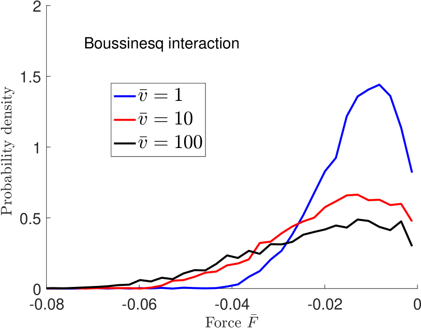
(a)

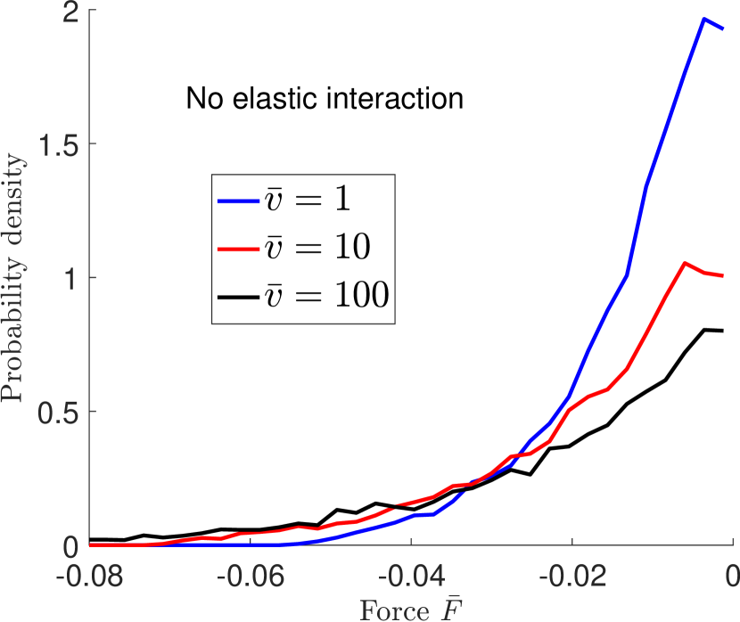
(b)

Figure 11: Force distribution at contacts at steady state at different sliding speeds. The area under the curve is less than $1$ since only a small percentage of the nominal area is in contact.

5.3 Decreasing contact area with increasing velocity

With increasing slip velocity, the steady-state dilatation always increases and the total contact area always decreases (Figure 12). The two timescales relevant to sliding contact are the viscoelastic relaxation timescale (determined by $\bar{\lambda}$) and the ratio of the correlation length to the sliding speed, $\bar{\beta}/\bar{v}$.

Apart from the surface roughness, the steady-state contact area at a given velocity depends on the viscoelastic properties. In static contact (section 4), the duration of friction evolution is determined by $\bar{\lambda}$ and the magnitude of the friction increase by $\bar{A}/\bar{\lambda}$ (Section 4.2). Instantaneous and steady-state behavior of the static contact is somewhat analogous to sliding at very high and very low velocity. Thus, $\bar{\lambda}$ is related to the range of slip velocities at which the system is velocity-dependent and $\bar{A}/\bar{\lambda}$ is related to the magnitude of the sensitivity. This is reflected in Figure 13(a) which shows the steady-state area as a function of the sliding speed for four combinations of $\bar{A},\bar{\lambda}$ and three values of $\bar{A}/\bar{\lambda}$ of 10, 1, and 0.1. Cases with the same value of $\bar{\lambda}$ but larger value of $\bar{A}/\bar{\lambda}$ have larger area changes over the velocity range shown. The two cases with the same $\bar{A}/\bar{\lambda}=1$, but different relaxation times of $\bar{\lambda}=1$ (blue line) and $\bar{\lambda}=0.1$ (purple line), have similar area changes for a range of slip velocities shifted by an order of magnitude; compare velocity ranges from 10 to 100 for $\bar{\lambda}=1$ (blue line) and from 1 to 10 for $\bar{\lambda}=0.1$ (purple line).

The average contact size remains approximately independent slip velocity (Figure 13(b)). With increasing velocity, the total contact area decreases but so do the number of contacts and the average contact size remains approximately the same. This is similar as in static contact where the average contact radius remains nearly constant with time under a constant total normal force (Figure 4(d)).

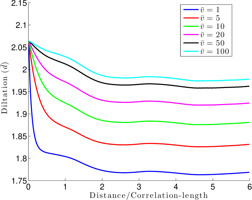
(a)

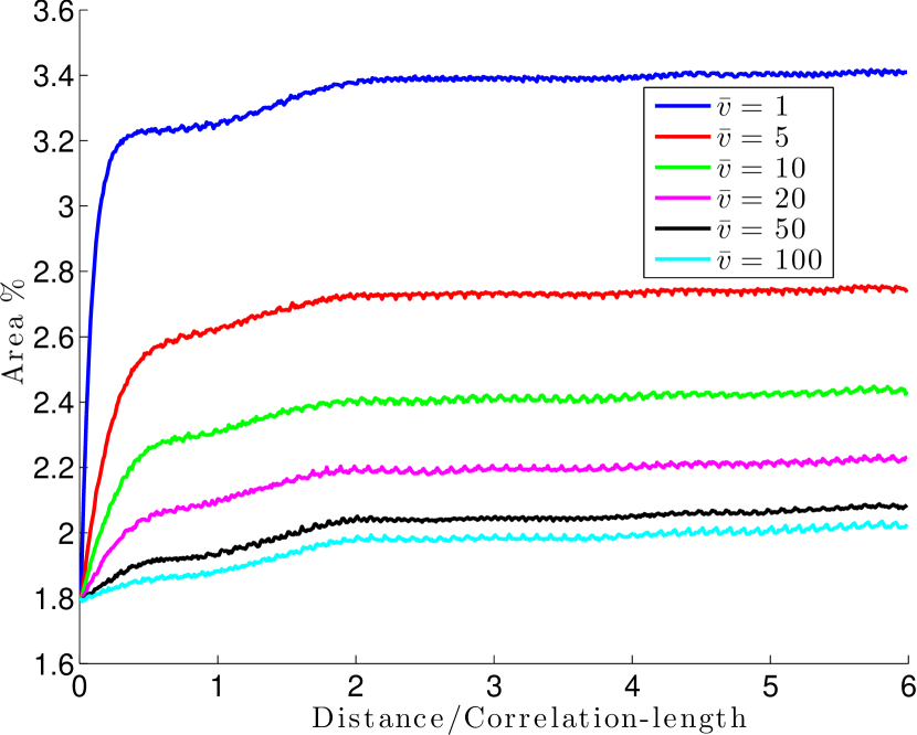
(b)

Figure 12: Evolution of (a) dilatation and (b) contact area starting from the same initial state and sliding at different speeds. At higher sliding speeds, the average force on a contact is higher and thus, to sustain the same global normal force, the dilatation is higher and the total area of contact is smaller.

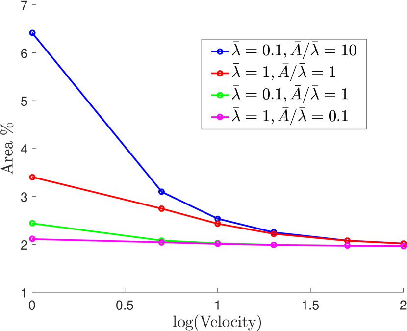
(a)

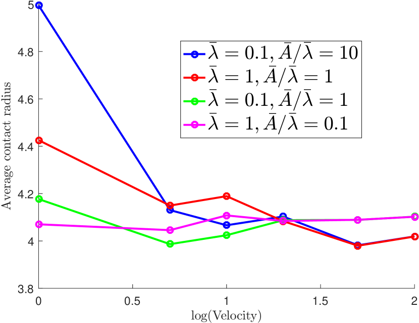
(b)

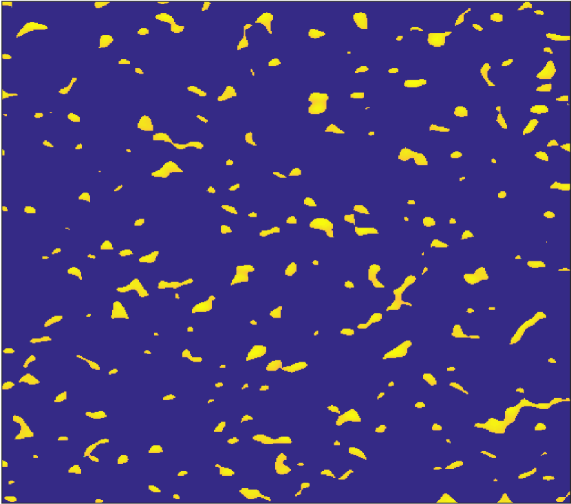
(c)

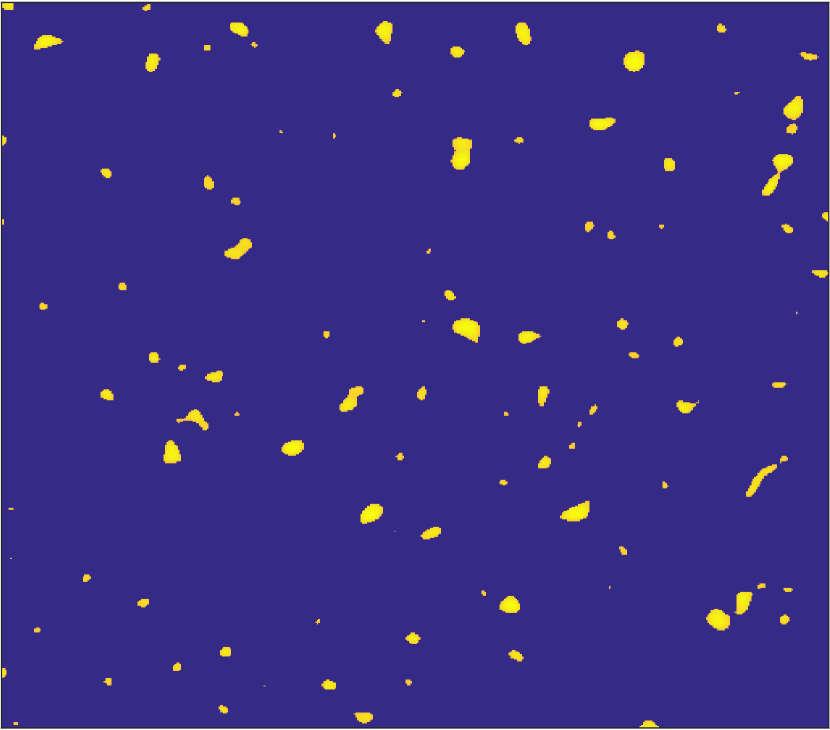
(d)

Figure 13: (a) Steady state contact area at different sliding speeds for four combinations of the viscoelastic parameters. The contact area always decreases with increasing speed. The magnitude of change and the velocities where $\mathrm{d}$Area/$\mathrm{d}$Velocity is large depends on the viscoelastic properties (see Section 5.3). (b) The average contact remains approximately constant with velocity. This is similar to the static contact case where the average contact size remained constant with time (Figure 4(d)). (c) and (d) show the contacts at steady state after sliding the same distance for velocities $\bar{v}=1$ and $\bar{v}=100$ (for the case $\bar{\lambda}=0.1,\bar{A}/\bar{\lambda}=10$). At $\bar{v}=1$, the total contact area is larger than that at $\bar{v}=100$ but so are the number of contacts and the average contact size remains approximately the same.

5.4 Comparison with experiments - velocity jump test

As in experiments, we perform velocity jump simulations. Two rough surfaces are brought into contact to a total force equivalent to a pressure of $100$ MPa. The surfaces are slid at this constant normal force at velocity $\bar{v}=10$ for the slip distance several times larger than the correlation length, to establish steady-state sliding. The sliding velocity is then instantaneously changed to $\bar{v}=1$. Jumps to $\bar{v}=10$ and $\bar{v}=1$ are repeated. Since the nondimensionalizing length and time scales are $1\mu$m and $1$ s, respectively, $\bar{v}=10$ corresponds to a sliding velocity of $10\mu$m/s, a typical value in experiments [7].

The resulting evolution of the macroscopic friction coefficient contains the direct and transient effects, as observed in experiments (Figure 14). The friction coefficient changes instantaneously with the velocity jumps because of the velocity-strengthening term in local shear resistance (14), and the change has the same sense as that of the velocity jump, i.e., the friction coefficient increases (decreases) when the velocity increases (decreases). Following the standard rate and state terminology, we call this jump the direct effect. The jump is followed by an evolution towards a steady state, because of the evolution of the real contact area. We call this evolution the transient. The transient changes the friction coefficient in the direction opposite to the direct effect, since the contact area decreases for higher velocities, as already discussed.

Even though the contact area always decreases with increasing sliding velocity, the steady-state friction coefficient can either increase or decrease, depending on whether the direct effect or the transient change dominates. If the transient is smaller than the direct effect, the steady-state friction is higher for higher velocity, resulting in velocity strengthening behavior. If the transient is larger than the direct effect, the steady-state value is lower for higher velocity, producing velocity weakening behavior. The area evolution depends on both the sliding velocity and viscoelastic properties. For given viscoelastic properties and a single relaxation timescale, the area evolution is largest for a certain range of velocities In part, the velocity dependence can transition between strengthening and weakening for different sliding velocities (Figure 14(d)). Such transitions have been observed in experiments as well [49]. However, some materials have been shown to be consistently velocity-weakening or velocity-strengthening for a wide range of sliding velocities. Such sustained behavior likely results from multiple relaxation timescales in the viscoelastic response.

The qualitative aspects of the sliding friction remain unchanged when the elastic interactions between elements are turned off. During sliding, the evolution of area and friction, velocity strengthening and velocity weakening, are determined largely by the viscoelastic properties and only quantitatively changed by the long-range elastic interactions.

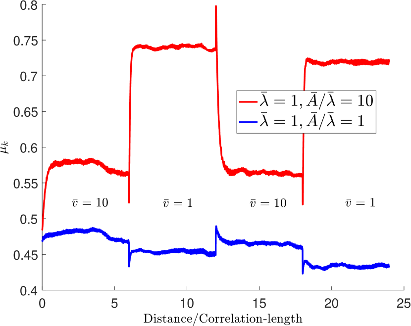
(a)

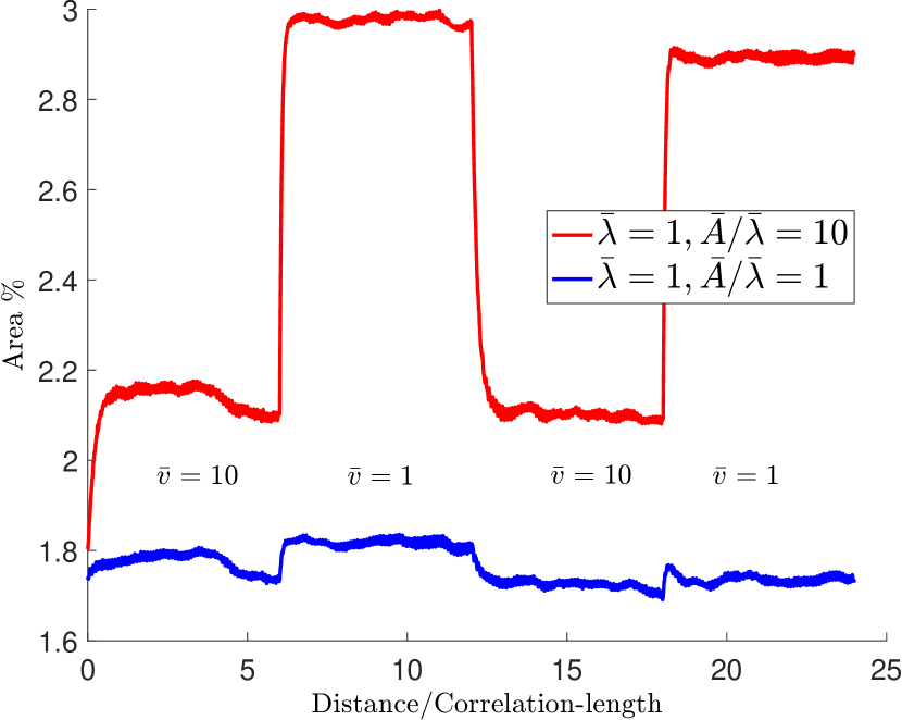
(b)

(c)

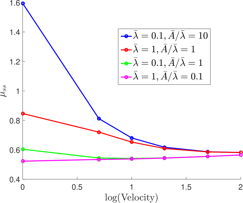
(d)

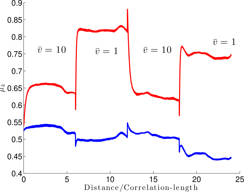
(e)

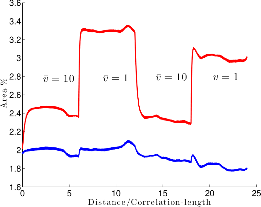
(f)

Figure 14: Evolution of (a) friction coefficient and (b) contact area during velocity jump tests with Boussinesq elastic interactions. Because of viscoelasticity, the average force on a contact is higher at higher speeds, and thus for the same global normal force, contact area is smaller at higher speeds. With a jump in sliding speed, $\mu_{k}$ changes instantaneously and this is followed by an evolution to a steady state. Depending on the material parameters, the steady state value can increase or decrease with increasing sliding speed. The two cases correspond to velocity strengthening (blue - $\bar{\lambda}=1,\bar{A}=1$ ) and velocity weakening (red - $\bar{\lambda}=1,\bar{A}=10$ ) respectively. (c) Evolution of contact area and friction during a velocity jump test (reproduced with permission from Dieterich [7]). (d) Steady state friction coefficient at different sliding speeds for four combinations of the viscoelastic parameters. The contact area always decreases with increasing speed but the friction coefficient might increase or decrease depending on whether the direct effect or the transient effect dominates. Evolution with no elastic interactions (e) and (f) is qualitatively similar to (a) and (b).

5.5 Macroscopic direct effect vs. microscopic hardening assumption

According to the assumed friction law (14) and the microscopic friction assumption (14), the magnitude of the direct effect for a velocity jump from $\bar{v}_{\text{old}}$ to $\bar{v}_{\text{new}}$ is given by

$$\Delta\mu_{\text{direct}}=\frac{\alpha\log(\bar{v}_{\text{new}}/\bar{v}_{\text{old}})\bar{A}(\bar{v}_{\text{old}})}{\bar{F}_{N}}.$$

Since $\bar{A}(\bar{v})$ decreases monotonically with increasing $\bar{v}$, the magnitude of the direct effect also decreases monotonically, for given $\bar{v}_{\text{new}}/\bar{v}_{\text{old}}$, if $\alpha$ is a constant. However, in experiments, it is observed that the direct effect remains constant over a large range of velocities [50]. This is possible only if the velocity-dependent term in the microscopic friction (14) increases faster than $\log(\bar{v})$. Moreover, the faster increase should exactly compensate for the evolution in the area, which is related to the viscoelastic properties. Note that this is a general observation based only on the assumption that the total shear force is proportional to the real area of contact, and it does not depend on any other particular features of our model.

5.6 Elasto/viscoplastic contacts

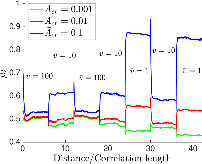
Figure 15: Evolution of $\mu_{k}$ during velocity jump tests for elasto/viscoplastic contacts. Larger creep rates lead to steady-state velocity-weakening friction while smaller creep rates result in steady-state velocity-strengthening behavior.

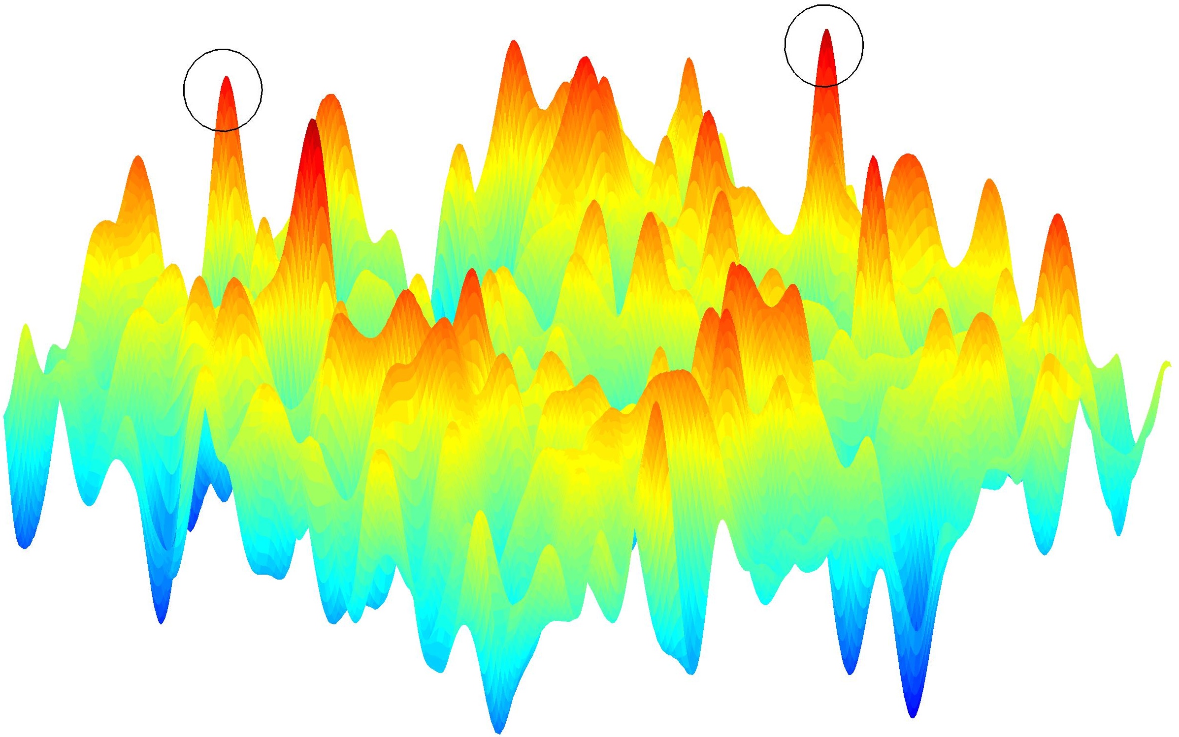
(a)

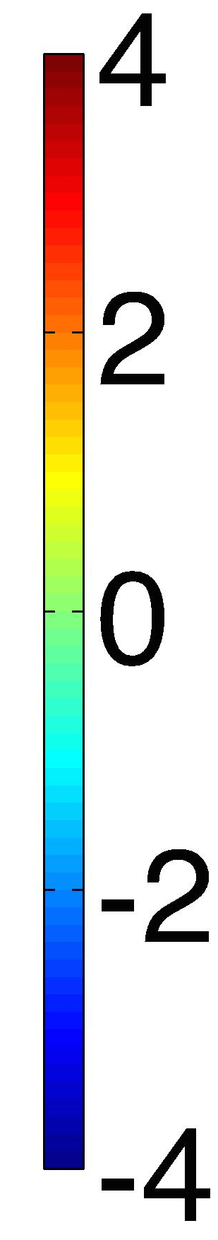
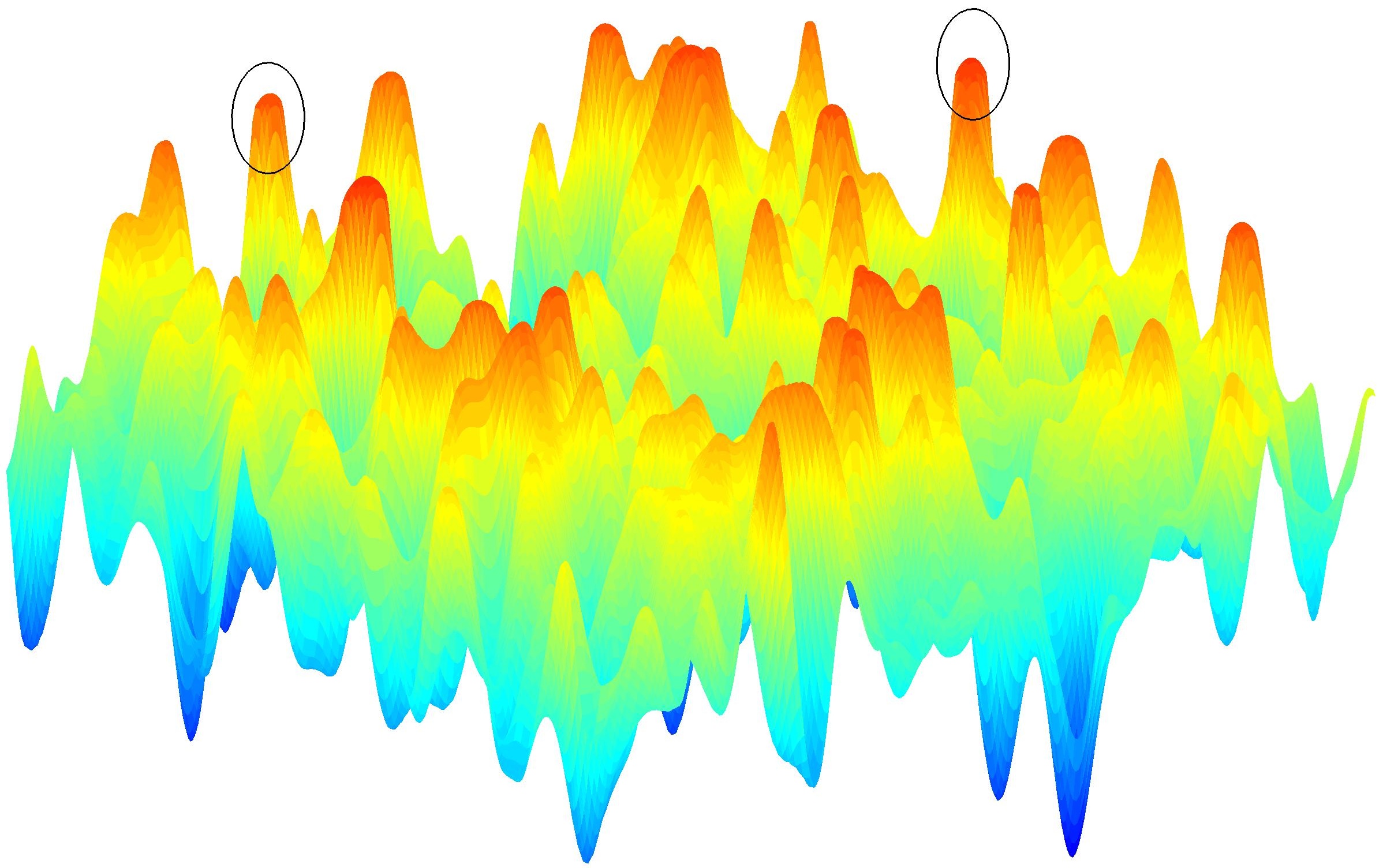
(b)

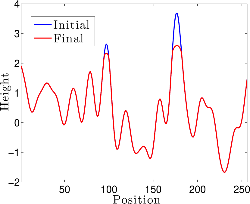
(c)

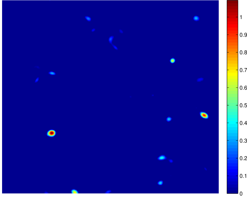
(d)

Figure 16: Evolution of the surface (i.e., $\bar{u}_{i}^{p}+\bar{h}(\bar{x}_{i}^{0}+\bar{x},\bar{y}_{i}^{0})$) during sliding: (a) initially undeformed and (b) final deformed surfaces. The blunting of the peaks due to permanent deformation is evident (black circles). (c) a profile showing a section across the surface and (d) plastic length changes at the contacts.

The qualitative features of the contact area and friction evolution described for the viscoelastic contacts in sections hold true for an elastic/viscoplastic constitutive assumption for the elements (Figure 15). As expected, the friction coefficient $\mu_{k}$ strongly depends on the creep rate $A_{cr}$. Larger creep rates lead to larger area changes, larger transients, and hence velocity weakening, whereas smaller creep rates result in velocity-strengthening behavior. Note that higher creep rates can be caused by higher temperatures [51]; however, higher temperatures also result in higher values for the microscopic rate-hardening of the contact friction (larger $\alpha$ in (14)), and the latter effect dominates at high enough temperatures in some materials ([52, 53, 54]).

One key difference between the viscoelastic and elasto/viscoplastic formulations is that, in the elasto/viscoplastic case, there is permanent deformation. So, the surfaces permanently change due to static or sliding contact. Figure 16 shows an example of the permanent surface change due to slip, with several peaks flattened due to slip, in particular, the two peaks marked with circles. The distribution of the plastic length change over the surface and a profile through the surface further illustrate the point.

This permanent change of the surface leads to history dependence and potentially carries a signature of the sliding direction. This is shown in Figure 17. One surface is slid over another for a certain distance and then the direction of sliding is reversed. We see that the dilatation decreases and the coefficient of friction increases on reversal. The deformable elements that pass over the highest peaks of the rigid surface get permanently deformed during forward motion and thus move closer and have higher contact area with the peaks on reverse motion.

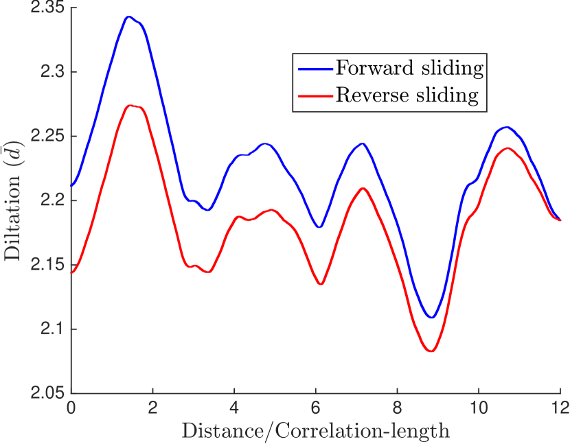
(a)

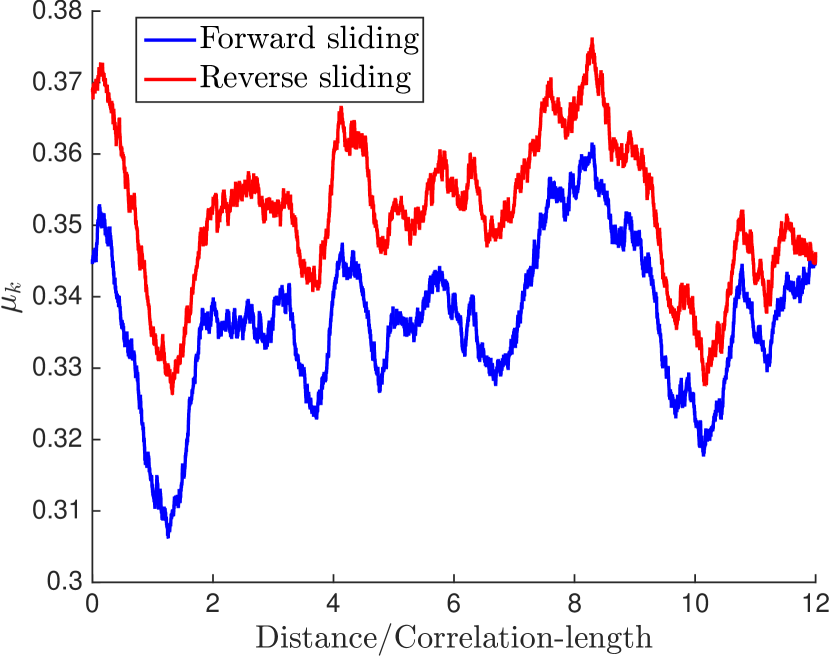
(b)

Figure 17: Evolution of dilatation and friction coefficient in forward and reverse sliding.

6 Conclusion

We have developed a numerical framework to study the time- and velocity-dependent behavior of viscoelastic and elasto/viscoplastic rough surfaces in static and sliding contact, including the long-range elastic interactions between contacts. We prescribe the material and surface properties at the microscale and infer the macroscopic friction behavior. We find that this framework reproduces main qualitative features of experimental observations. Further, our framework is able to identify which factors conceptually influence the macroscopic behavior and which ones are lost in the averaging process. Surprisingly, we find that, in both static and sliding contact in our models, long-range elastic interactions do not change the main qualitative aspects of macroscopic friction, although they are important from a quantitative perspective.

In static contact, both viscoelastic and elasto/viscoplastic surfaces exhibit an increase in static friction that is widely observed in experiments. In our models, this is achieved through creep-induced contact area increases. For viscoelastic surfaces, the duration of friction growth is determined by the viscoelastic relaxation times; multiple relaxation times scales are needed to reproduce the sustained increase in static friction coefficient with the logarithm of time observed in the laboratory experiments on some materials such as rocks ([5]). For viscoplastic surfaces, the growth persists without saturation, in the absence of hardening. In both cases, the rate of growth can be related to the viscoelastic and viscoplastic properties. Surface roughness plays an important role in determining the absolute contact area and thus friction, but it does not change either the duration or the amount of the friction increase during static contact.

During sliding with velocity jumps, both viscoelastic and elasto/viscoplastic surfaces show the direct and transient effects as observed in the laboratory. The direct effect in our models arises from the assumed velocity-strengthening shear strength of contacts. For an abrupt velocity increase/decrease, the total contact area remains constant, but the shear resistance abruptly increases/decreases. However, larger sliding velocities correspond to smaller steady-state contact areas, because the average normal force on a contact increases with the sliding velocity. Hence, after a velocity jump, the contact area evolves, leading to the transient effect. Depending on the amplitude of the direct effect and how the contact area evolves for different material properties and sliding velocities, the steady-state friction response can be velocity strengthening or velocity weakening. In our model, as in the previous theoretical studies [28, 29], the evolution of the contact area provides the physical basis for the state variable used in empirical rate-and-state models. An important difference between viscoelastic and elasto/viscoplastic surfaces is that plasticity leads to permanent changes in the surface profile.

To reproduce the more specific features encapsulated in the empirical rate-and-state formulations (Equations 2-3), our model would require more involved constitutive models for both the deforming elements and for the microscopic shear strength of contacts. In the viscoelastic models with a single relaxation time scale explored in this study, the area change is substantial for a certain range of sliding velocities. As higher velocities are imposed, the area change decreases and eventually disappears, effectively corresponding to parameter $b$ from the empirical rate-and-state laws (Equations 2-3) being a function of sliding velocity $v$. This leads to velocity-strengthening behavior at high enough sliding velocities, due to the presence of the direct effect. Such transition to velocity-strengthening behavior at higher velocities have been observed in some experiments ([49]), but many materials display velocity-weakening friction over several orders of magnitude in sliding velocities, with the transient effect being proportional to the logarithm of the velocity jump ([55]). We hypothesize that such sustained velocity-weakening behavior can be achieved in our model by including multiple shorter relaxation time scales.

Furthemore, the macroscopic direct effect in our model is not proportional to the logarithm of the velocity jump, as observed in many experiments, but it is modulated by the area changes with sliding velocity. In other words, our model results in parameter $a$ of (2-3) that depends on the contact area and hence $a$ is also a function of $v$. Since the evolution of the total contact area with sliding velocity is a robust feature of our model, this discrepancy cannot be fixed by simply changing the constitutive properties of the elements, e.g, adding additional relaxation time scales. Rather, this discrepancy signifies the need to a more sophisticated shear strength assumption on the microscale, one that reflects the assumed constitutive properties of the bulk material.

Our model assumes local shear resistance that does not depend on the individual conditions of the element in contact, and all elements are assumed to move with the same macroscopic sliding velocity. Hence, the evolving asperity population affects the macroscopic friction only through the evolution of the total contact area. The developed numerical framework can be used to study the consequences of relaxing this assumption. One idea that can be explored in our framework is that the local shear resistance increases with the local time in contact (or contact maturity), due to local processes allowing for better atomic scale matching, desorption of trapped impurities, etc [43]. This would make the local shear resistance depend not only on the sliding velocity but also on the (evolving) individual asperity size, with larger asperities being stronger per unit area. Another possibility to explore is that the local shear resistance depends on the local state of the element, e.g., its normal force. In both cases, the evolution of macroscopic friction, and hence the effective state variable, may no longer be primarily dependent on the evolution of the total contact area, but additionally reflect the variation in the distribution of the contact sizes and forces. Such a modification would enhance the importance of the surface roughness in controlling the macroscopic friction behavior. In such models, the long-range elastic interactions may become more conceptually important, since our simulations show that they significantly affect the distribution of the contact forces and asperity sizes.

Finally, we use a Gaussian autocorrelation function, while natural surfaces are thought to be fractal. We have done some preliminary studies on surfaces with an exponential autocorrelation,

$$R_{zz}(\delta_{x},\delta_{y})=\mathrm{E}\{z(x,y)z(x+\delta_{x},y+\delta_{y})\}=\sigma^{2}e^{-(\delta_{x}^{2}+\delta_{y}^{2})^{1/2}/\beta},$$

where $\beta$ is the correlation length. The power spectral density for this surface is given by,

$$S(\omega_{x},\omega_{y})=\frac{2\pi\sigma^{2}\beta^{2}}{\left[1+\left(\omega_{x}^{2}+\omega_{y}^{2}\right)\beta^{2}\right]^{3/2}}.$$ (18)

So, if $\left(\omega_{x}^{2}+\omega_{y}^{2}\right)^{1/2}\beta\gg 1$, the power spectrum decays as $1/\omega^{3}$ (where $\omega=(\omega_{x}^{2}+\omega_{y}^{2})^{1/2}$) which corresponds to a fractal dimension of $2.5$ (or a Hurst exponent of $0.5$). We have verified that the qualitative friction behavior during both static/sliding contact remains the same as in the Gaussian autocorrelation case. However, a detailed parameter study, as well as the study of other fractal surfaces remains a topic of future work.

To summarize, various experimentally observed features of friction – growth of the static friction coefficient with time, velocity and history dependence of the dynamic friction coefficient, velocity-strengthening and velocity-weakening behavior of steady-state friction – can be captured by a bare minimum of ingredients, a time-dependent and velocity-dependent contact at the microscale with statistical averaging due to rough surfaces. The main qualitative aspects of the evolution are the same in the viscoelastic and elasto/viscoplastic cases, showing that the macroscopic frictional response is robust with respect to a wide range of microscopic material behavior. The developed framework can be used to study which assumption on the microscale produce the specific features of the macroscopic behavior captured in empirical rate-and-state laws.

References

- [1] S. Hulikal, K. Bhattacharya, and N. Lapusta. Collective behavior of viscoelastic asperities as a model for static and kinetic friction. Journal of the Mechanics and Physics of Solids, 76:144–161, 2015.
- [2] R. Holm and E.A. Holm. Electric contacts. Springer, 1967.
- [3] F.P. Bowden and D. Tabor. The friction and lubrication of solids. Clarendon Press, 1986.
- [4] E. Rabinowicz. Friction and wear of materials, volume 2. Wiley New York, 1965.
- [5] J. H. Dieterich. Time-dependent friction in rocks. Journal of Geophysical Research, 77:3690–97, 1972.
- [6] J. H. Dieterich. Time-dependent friction and the mechanics of stick-slip. Pure and Applied Geophysics, 116:790–806, 1978.
- [7] J. H. Dieterich and B. D. Kilgore. Direct observation of frictional contacts: New insights for state-dependent properties. Pure and Applied Geophysics, 143:283–302, 1994.
- [8] J. H. Dieterich. Modeling of rock friction 1. Experimental results and constitutive equations. Journal of Geophysical Research, 84:2161–2168, May 1979.
- [9] A.L. Ruina. Slip instability and state variable friction laws. Journal of Geophysical Research, 881:10359–10370, 1983.
- [10] S.T. Tse and J.R. Rice. Crustal earthquake instability in relation to the depth variation of frictional slip properties. Journal of Geophysical Research: Solid Earth (1978–2012), 91:9452–9472, 1986.
- [11] J.H. Dieterich. Applications of rate-and state-dependent friction to models of fault slip and earthquake occurrence. Treatise on Geophysics, 4:107–129, 2007.
- [12] Y. Kaneko, J-P. Avouac, and N. Lapusta. Towards inferring earthquake patterns from geodetic observations of interseismic coupling. Nature Geoscience, 3:363–369, 2010.
- [13] S. Barbot, N. Lapusta, and J-P. Avouac. Under the hood of the earthquake machine: toward predictive modeling of the seismic cycle. Science, 336:707–710, 2012.
- [14] H. Noda and N. Lapusta. Stable creeping fault segments can become destructive as a result of dynamic weakening. Nature, 493:518–521, 2013.
- [15] A.L. Ruina. Stability of steady frictional slipping. Journal of applied mechanics, 50:343–349, 1983.
- [16] W. Yan and K. Komvopoulos. Contact analysis of elastic-plastic fractal surfaces. Journal of Applied Physics, 84:3617–3624, 1998.
- [17] S. Hyun, L. Pei, J-F. Molinari, and M.O. Robbins. Finite-element analysis of contact between elastic self-affine surfaces. Physical Review E, 70:026117, 2004.
- [18] P.K. Gupta and J.A. Walowit. Contact stresses between an elastic cylinder and a layered elastic solid. Journal of Tribology, 96:250–257, 1974.
- [19] M.N. Webster and R.S. Sayles. A numerical model for the elastic frictionless contact of real rough surfaces. Journal of Tribology, 108:314–320, 1986.
- [20] N. Ren and S.C. Lee. Contact simulation of three-dimensional rough surfaces using moving grid method. Transactions - American Society of Mechanical Engineers. Journal of Solar Energy Engineering, 115:597–597, 1993.
- [21] Y. Ju and T.N. Farris. Spectral analysis of two-dimensional contact problems. Journal of Tribology, 118:320–328, 1996.
- [22] I.A. Polonsky and L.M. Keer. A Fast and Accurate Method for Numerical Analysis of Elastic Layered Contacts. Journal of tribology, 122, 2000.
- [23] G. Liu, Q. Wang, and S. Liu. A three-dimensional thermal-mechanical asperity contact model for two nominally flat surfaces in contact. Journal of Tribology, 123:595–602, 2001.
- [24] C.K. Bora, M.E. Plesha, and R.W. Carpick. A numerical contact model based on real surface topography. Tribology Letters, 50:331–347, 2013.
- [25] Y. Bréchet and Y. Estrin. The effect of strain rate sensitivity on dynamic friction of metals. Scripta metallurgica et materialia, 30:1449–1454, 1994.
- [26] Y Estrin and Y Bréchet. On a model of frictional sliding. Pure and Applied Geophysics, 147:745–762, 1996.
- [27] P. Berthoud, T. Baumberger, C. G’sell, and J-M. Hiver. Physical analysis of the state-and rate-dependent friction law: Static friction. Physical Review B, 59:14313, 1999.
- [28] T. Baumberger, P. Berthoud, and C. Caroli. Physical analysis of the state- and rate-dependent friction law. ii. dynamic friction. Phys. Rev. B, 60:3928–3939, Aug 1999.
- [29] T. Putelat, H.P.D. Dawes, and J.R. Willis. On the microphysical foundations of rate-and-state friction. Journal of the Mechanics and Physics of Solids, 59:1062 – 1075, 2011.
- [30] J. F. Archard. Elastic deformation and the laws of friction. Proceedings of the Royal Society of London. Series A. Mathematical and Physical Sciences, 243(1233):190–205, 1957.
- [31] J.A. Greenwood and J.B.P. Williamson. Contact of nominally flat surfaces. Proceedings of the Royal Society of London. Series A., 295:300–319, 1966.
- [32] A. Majumdar and B. Bhushan. Fractal model of elastic-plastic contact between rough surfaces. Journal of Tribology, 113:1–11, 1991.
- [33] T. Thomas. Rough surfaces, second edition. London: Imperial College Press, 1999.
- [34] M.S. Longuet-Higgins. The statistical analysis of a random, moving surface. Philosophical Transactions of the Royal Society of London. Series A, 249:321–387, 1957.
- [35] Richard S Sayles and Tom R Thomas. Surface topography as a nonstationary random process. Nature, 271:431–434, 1978.
- [36] P.R. Nayak. Random process model of rough surfaces. Journal of Lubrication Technology, 93:398, 1971.
- [37] P.R. Nayak. Random process model of rough surfaces in plastic contact. Wear, 26:305–333, 1973.
- [38] D.J. Whitehouse and J.F. Archard. The properties of random surfaces of significance in their contact. Proceedings of the Royal Society of London. A, 316:97–121, 1970.
- [39] H.C. Kim and T.P. Russell. Contact of elastic solids with rough surfaces. Journal of Polymer Science Part B: Polymer Physics, 39:1848–1854, 2001.
- [40] Y.Z. Hu and K. Tonder. Simulation of 3-d random rough surface by 2-d digital filter and fourier analysis. International Journal of Machine Tools and Manufacture, 32:83–90, 1992.
- [41] A.F. Bower. Applied Mechanics of Solids. Taylor and Francis, 2012.
- [42] A.E.H Love. The stress produced in a semi-infinite solid by pressure on part of the boundary. Philosophical Transactions of the Royal Society of London. Series A, pages 377–420, 1929.
- [43] J.R. Rice, N. Lapusta, and K. Ranjith. Rate and state dependent friction and the stability of sliding between elastically deformable solids. Journal of the Mechanics and Physics of Solids, 49:1865 – 1898, 2001.
- [44] S. Balay, Abhyankar.S., M.F. Adams, J. Brown, P. Brune, K. Buschelman, V. Eijkhout, W.D. Gropp, K. Kaushik, M.D. Knepley, L.D. McInnes, K. Rupp, B.F. Smith, and H. Zhang. PETSc Web page. http://www.mcs.anl.gov/petsc, 2014.
- [45] L. Greengard and V. Rokhlin. A fast algorithm for particle simulations. Journal of Computational Physics, 73:325–348, 1987.
- [46] A.T. Ihler. An overview of fast multipole methods. Area Exam, 2004.
- [47] James H Dieterich and Brian D Kilgore. Imaging surface contacts: power law contact distributions and contact stresses in quartz, calcite, glass and acrylic plastic. Tectonophysics, 256(1):219–239, 1996.
- [48] R.S.H. Richardson and H. Nolle. Surface friction under time-dependent loads. Wear, 37:87–101, 1976.
- [49] T. Shimamoto. Transition between frictional slip and ductile flow for halite shear zones at room temperature. Science, 231:711–714, 1986.
- [50] MF Linker and JH Dieterich. Effects of variable normal stress on rock friction: Observations and constitutive equations. Journal of Geophysical Research: Solid Earth (1978–2012), 97(B4):4923–4940, 1992.
- [51] H.J. Frost and M.F Ashby. Deformation mechanism maps: the plasticity and creep of metals and ceramics. Pergamon Press, 1982.
- [52] M.L. Blanpied, D.A. Lockner, and J.D. Byerlee. Fault stability inferred from granite sliding experiments at hydrothermal conditions. Geophysical Research Letters, 18:609–612, 1991.
- [53] M.L. Blanpied, D.A. Lockner, and J.D. Byerlee. Frictional slip of granite at hydrothermal conditions. Journal of Geophysical Research: Solid Earth, 100:13045–13064, 1995.
- [54] C.H. Scholz. The mechanics of earthquakes and faulting. Cambridge university press, 2002.
- [55] C. Marone. Laboratory-derived friction laws and their application to seismic faulting. Annual Review of Earth and Planetary Sciences, 26:643–696, 1998.