BRST invariant RG flows

Abstract

A mass parameter for the gauge bosons in gauge-fixed four-dimensional Yang-Mills theory can be accommodated in a local and manifestly BRST-invariant action. The construction is based on the Faddeev-Popov method involving a nonlinear gauge-fixing and a background Nakanishi-Lautrup field. When applied to momentum-dependent masslike deformations, this formalism leads to a full regularization of the theory which explicitly preserves BRST symmetry. We deduce a functional renormalization group equation for the one-particle-irreducible effective action, which has a one-loop form. The master equation is compatible with it, i.e. BRST symmetry is preserved along the flow, and it has a standard regulator-independent Zinn-Justin form. As a first application, we compute the leading-order gluon wave-function renormalization.

I Introduction

The fact that global symmetries can be implemented exactly is one of the cornerstones of many qualitative and quantitative successes of functional continuum methods in quantum field theory. A prime example is chiral symmetry which can exactly be accounted for even in the presence of ultraviolet (UV) and infrared (IR) regularizations as formulated in the framework of the functional renormalization group (RG) Wetterich (1993); Bonini et al. (1993); Ellwanger (1994a); Morris (1994). By contrast, local gauge symmetries, as well as nonlinear or diffeomorphism symmetries, require a more careful discussion, as a symmetry transformation can arbitrarily mix modes in momentum space. This seems naturally in conflict with regularizations that operate locally in momentum space. A elementary example is given by a mass term for the gauge boson which would provide for an IR regularization, but breaks gauge invariance.

In standard continuum formulations, quantization of gauge theories, such as Faddeev-Popov quantization, involves a gauge-fixing procedure in order to remove the large redundancy in the space of field configurations to be integrated over. This goes along with explicit symmetry-breaking terms. While gauge-invariant observables are not affected by the details of the gauge-fixing procedure, gauge-variant building blocks such as gauge-field correlation functions and vertices do depend on the gauge choice. The underlying symmetry is still encoded in Ward-Takahashi identities that relate these correlation functions also across loop orders. While the computation of gauge-invariant observables out of gauge-variant building blocks such as correlation functions thereby remains conceptually possible, it becomes technically more demanding.

A major simplification arises from BRST symmetry, a remnant global supersymmetry that nonlinearly mixes gauge, Faddeev-Popov ghost and further auxiliary fields Becchi et al. (1975, 1976); Tyutin (1975). BRST symmetry not only helps identifying the physical Hilbert space of states but also simplifies the constraint equation for correlation functions in the form of the Zinn-Justin master equation Zinn-Justin (1975a, b). At the expense of auxiliary sources, the Zinn-Justin equation relates correlation functions algebraically. I.e., its resolution can be approached by algebraic cohomology methods and does not require the computation of loop terms.

In the presence of a generic momentum-space regularization, the elegance (and practicality) of the master equation is no longer present. For functional RG flows, it has been shown by Ellwanger Ellwanger (1994b) that gauge invariance of correlation functions as summarized by the effective action can still be encoded in a master equation. However, the regularization procedure which is generically encoded on the level of the propagator leads to additional regulator-dependent terms in the master equation (modified Slavnov-Taylor identities) which again correspond to loop terms. Whereas this modified master equation, as well as a corresponding additional modified Ward-Takahashi identity Bonini et al. (1994); D’Attanasio and Morris (1996); Litim and Pawlowski (1999, 1998), encodes the constraints imposed by the symmetries on a conceptually satisfactory level Pawlowski (2007); Gies (2012), it increases the level of technical complexity for nonperturbative approximation schemes, cf. Ellwanger et al. (1996, 1998). Direct applications of functional RG flows together with a resolution of the modified master equation beyond perturbation theory have remained rare Ellwanger et al. (1996, 1998); Gies et al. (2004); Fischer and Gies (2004); Fejos and Hatsuda (2017), though the intricacies can simplify in certain gauges such as the Landau gauge Fischer et al. (2009); Cyrol et al. (2016).

Several schemes have been devised, to tackle this practical problem. For instance, an alternative approach has been developed in Igarashi et al. (2000); Sonoda (2007); Igarashi et al. (2007, 2016) introducing a deformed BRST symmetry that includes the regulator and reduces to standard BRST symmetry in the suitable limits. This formulation indeed encodes gauge invariance even of the regularized theory in a bilinear master equation, but at the same time makes the nonlocality of gauge symmetry in momentum space manifest. A convenient scheme to devise nonperturbative approximations relies on the use of background-field methods Reuter and Wetterich (1994a), where invariance under background-field transformations can rather straightforwardly be obtained. Nevertheless, the true quantum gauge invariance is again encoded in modified symmetry identities (Nielsen identities, shift-Ward identity) Reuter and Wetterich (1994b, 1997); Freire et al. (2001, 2000); Pawlowski (2007); Bridle et al. (2014); Becker and Reuter (2014); Dietz and Morris (2015); Percacci and Vacca (2017); Safari and Vacca (2017, 2016), which in practice have been largely treated on an approximate level Reuter and Wetterich (1994b, 1997); Gies (2002); Braun et al. (2010); Eichhorn et al. (2011).

Several further directions have been explored in this context: a manifestly gauge-invariant RG flow has been proposed in Morris (1998) and further developed in Arnone et al. (2002, 2003, 2007) which does not rely on Faddeev-Popov quantization, but makes use of an embedding into an SU($N|N$) supergauge theory. A variety of results has been obtained Arnone et al. (2004, 2005) including a gauge-invariant computation of the two-loop $\beta$ function Morris and Rosten (2006a, b); Evans et al. (2006); Rosten (2012). Gauge-invariant RG flows for the geometric effective action have also been set up within the Vilkovisky-DeWitt framework Branchina et al. (2003); Pawlowski (2003) with application in the asymptotic-safety scenario for quantum gravity Donkin and Pawlowski (2012). A gauge-invariant RG flow has also recently been constructed in Wetterich (2016, 2018) making use of physical gauges and the freedom to suitably define the macroscopic field and the effective action. Despite these conceptually successful implementations of gauge invariance in RG flows, the most advanced applications to nonperturbative questions often rely on the standard Faddeev-Popov quantization as this has remained technically more accessible for sophisticated systematic expansion schemes, cf. Cyrol et al. (2016); Denz et al. (2018); Cyrol et al. (2018); Corell et al. (2018).

In the present work, we suggest a novel approach for the construction of RG flows for gauge systems that relies on Faddeev-Popov quantization and aims at preserving exact BRST symmetry. The key idea is to treat the regularization as a contribution to the gauge fixing. As this is not possible within linear gauges, we consider a special choice of a nonlinear (quadratic) gauge condition. BRST symmetry in the standard fashion remains manifest at all stages of the construction. In order to obtain a conventional regulator term for the gauge field, we use a Fourier noise field for the Nakanishi-Lautrup auxiliary field. As a new ingredient, this gives rise to a background Nakanishi-Lautrup field.

Also the ghost sector is at variance with that of standard linear gauges while preserving exact BRST invariance. In particular, new regulator-dependent vertices appear. Nevertheless, gauge invariance gives rise to a master equation for the (Legendre) effective action which can be brought to standard form with the aid of two additional source fields. This facilitates the resolution of the symmetry constraints by conventional algebraic cohomology methods. Most importantly, the resulting functional nonperturbative flow equation for the effective action has a one-loop structure and is thus amenable to widely used nonperturbative approximation schemes.

The paper is organized as follows. In Sec. II, we set the stage by recalling basics of gauge-fixed functional integrals in order to introduce our conventions. We introduce the Nakanishi-Lautrup auxiliary field in Sec. III together with a convenient choice of a corresponding noise field which is advantageous for our formalism. Sec. IV is devoted to a discussion of constructing a simple nonlinear gauge that allows to write down an action with BRST-invariant mass terms; since this is a rather widely discussed topic in the literature, this section might be of interest in its own right. Here, we use it as a motivation for the construction of a BRST-invariant RG flow. The latter is presented in Sec. V, where we derive the one-loop functional RG flow equation. The master equation encoding BRST invariance and its RG flow is discussed in Sec. VI. Here, we give an explicit proof of the compatibility between the master equation and the flow equation, i.e. an action that satisfies the master equation at an initial scale will do so on all scales, provided it also satisfies the flow equation that links the two scales. The question concerning the well posedness of the functional regularization obtained through a nonlinear gauge fixing is addressed in Sec. VII, where we analyze the mapping between the effective action and the bare action, and the choice of RG initial conditions. A simple application of the functional flow equation to one-loop order is presented in Sec. VIII. Auxiliary information is presented in three appendices.

II Conventions

In this work, we discuss pure Yang-Mills theory in $d$-dimensional Euclidean spacetime, using the gauge field $A_{\mu}^{a}(x)$ in the adjoint representation of the gauge group $G$ as the local field degree of freedom. For the counting of canonical dimensions, we implicitly use $d=4$ as an illustration. Other than that, our formalism applies to general $d$. The inclusion of charged matter fields is straightforward. The use of the gauge field entails a large redundancy manifested by the invariance under local (infinitesimal) gauge transformations, $\delta A_{\mu}^{a}(x)=\left(D_{\mu}\omega\right)^{a}(x)$ for infinitesimal $\omega^{a}(x)$. Here, we use the covariant derivative in the adjoint representation,

$$D_{\mu}^{ab}=\partial_{\mu}\delta^{ab}+gf^{abc}A_{\mu}^{c}\,.$$ (1)

We use condensed notation such that color indices replace also spacetime indices, and the summation convention over these repeated indices is extended to integration over the corresponding spacetime points, whenever two identical indices both refer to field variables. E.g., the covariant derivative then reads

$$D_{\mu}^{ab}(x_{a},x_{b})=\left(\delta^{ab}\partial_{\mu}+gf^{abc}A_{\mu}^{c}(x_{a})\right)\delta(x_{a}-x_{b})\,.$$ (2)

Finite gauge transformations can be written as

$$A_{\mu}^{\omega}=UA_{\mu}U^{-1}-\frac{\mathrm{i}}{g}\left(\partial_{\mu}U\right)U^{-1}\,,\quad A_{\mu}=A_{\mu}^{a}T^{a},$$ (3)

where

$$U(\omega)=e^{-\mathrm{i}g\omega^{a}T^{a}}\in G\,,$$ (4)

with general finite $\omega^{a}(x)$ and generators

$$\left[T^{a},T^{b}\right]=\mathrm{i}f^{abc}T^{c}\,.$$ (5)

The field strength reads

$$F^{a}_{\mu\nu}=\partial_{\mu}A_{\nu}^{a}-\partial_{\nu}A_{\mu}^{a}+gf^{abc}A_{\mu}^{b}A_{\nu}^{c},$$ (6)

with adjoint indices $a,b,c\dots$. In condensed notation, the Yang-Mills action is given by

$$S_{\mathrm{YM}}[A]=\frac{1}{4}F_{\mu\nu}^{a}F^{a\mu\nu}\,.$$ (7)

For quantization, we introduce a gauge-fixing functional $\mathsf{F}^{a}[A]$, playing a central role for the Faddeev-Popov method:

$$1=\int\!\mathcal{D}\mathsf{F}^{a}\,\delta[\mathsf{F}^{a}]=\int\!\mathrm{d}\mu(\omega)\,\delta\left[\mathsf{F}^{a}[A^{\omega}]\right]\Delta_{\mathrm{FP}}\left[A^{\omega}\right]\,,$$ (8)

where $\mathrm{d}\mu$ is the Haar measure and

$$\Delta_{\mathrm{FP}}\left[A^{\omega}\right]=\mathrm{Det}\frac{\delta\mathsf{F}^{a}[A^{\omega}]}{\delta\omega^{b}}\,,$$ (9)

is the Faddeev-Popov determinant. The latter is gauge invariant, so that we can replace $A^{\omega}$ with $A$. This determinant can be written in terms of a local action $S_{\mathrm{gh}}$ by means of ghost fields

$$\Delta_{\mathrm{FP}}[A]=\int\!\!\mathcal{D}\bar{c}\,\mathcal{D}c\,e^{-S_{\mathrm{gh}}[A,c,\bar{c}]}\,.$$ (10)

Imposing a strict gauge-fixing condition is not necessary, because replacing

$$\delta\left[\mathsf{F}^{a}[A^{\omega}]\right] \longrightarrow B\left[\mathsf{F}^{a}[A^{\omega}]\right]$$ (11)

simply changes the $1$ on the left-hand side of Eq. (8) into a constant. The standard textbook example is

$$B\left[\mathsf{F}^{a}[A]\right]=e^{-S_{\mathrm{gf}}[A]}\,,$$ (12)

based on a local gauge-fixing contribution to the action,

$$S_{\mathrm{gf}}[A]=\frac{1}{2\xi}\mathsf{F}^{a}[A]\mathsf{F}^{a}[A],$$ (13)

with gauge parameter $\xi$.

Baring explicit breakings through the gauge condition, the global $G$ symmetry remains intact even after gauge fixing. E.g., the ghosts transform under the adjoint of the global $G$ group, i.e. $\omega=\text{const.}$,

$$\begin{split}\delta c^{a}&=gf^{abc}\omega^{b}c^{c}\,,\\ \delta\bar{c}^{a}&=gf^{abc}\omega^{b}\bar{c}^{c}\,.\end{split}$$ (14)

We can associate a set of generators to both local gauge and global color rotations given by

$$\mathcal{G}^{a}(x)=\mathcal{G}^{a}_{A}(x)+\mathcal{G}^{a}_{\mathrm{gh}}(x)\,,$$ (15)

where

$$\begin{split}\mathcal{G}^{a}_{A}(x)&=D_{\mu}^{ab}\frac{\delta}{\delta A_{\mu}^{b}},\\ \mathcal{G}^{a}_{\mathrm{gh}}(x)&=-gf^{abc}\left(c^{c}\frac{\delta}{\delta c^{b}}+\bar{c}^{c}\frac{\delta}{\delta\bar{c}^{b}}\right).\end{split}$$ (16)

All functional derivatives in this paper are left derivatives by default, unless otherwise specified. The gauge action $S_{\mathrm{gf}}+S_{\mathrm{gh}}$ emerging from the Faddeev-Popov construction exhibits an additional global (super-)symmetry: BRST symmetry. Introducing a Grassmannian BRST operator $s$ acting on the fields, the BRST transforms read

$$\begin{split}\left(sA\right)^{a}_{\mu}&=D_{\mu}^{ab}c^{b},\\ \left(sc\right)^{a}&=\frac{1}{2}gf^{abc}c^{b}c^{c},\\ \left(s\bar{c}\right)^{a}&=-\frac{1}{\xi}\mathsf{F}^{a}.\\ \end{split}$$ (17)

As the BRST transform of the gauge potential has the form of a gauge transformation, any gauge-invariant contribution to the action is guaranteed to be BRST invariant.

Quantization now proceeds straightforwardly through the generating functional

$$Z[J,\eta,\bar{\eta}]=e^{W[J,\eta,\bar{\eta}]}=\int\!\mathcal{D}A\mathcal{D}c\mathcal{D}\bar{c}\,e^{-S_{\mathrm{tot}}}\,,$$ (18)

with the total action

$$S_{\mathrm{tot}}[A,c,\bar{c},J,\eta,\bar{\eta}] = S_{\mathrm{YM}}[A]+S_{\mathrm{gh}}[A,c,\bar{c}]+S_{\mathrm{gf}}[A]$$ (19)

$$+S_{\mathrm{so}}[A,c,\bar{c},J,\eta,\bar{\eta}]\,.$$

The source terms are summarized in

$$S_{\mathrm{so}}[A,c,\bar{c},J,\eta,\bar{\eta}]=-\left(J^{a\mu}A^{a}_{\mu}+\bar{\eta}^{a}c^{a}+\bar{c}^{a}\eta^{a}\right).$$ (20)

By Legendre transformation, the effective action can be constructed from the Schwinger functional $W[J,\eta,\bar{\eta}]$,

$$\Gamma[A,c,\bar{c}]=\mathop{\text{sup}}_{J,\eta,\bar{\eta}}\left\{J^{a\mu}A_{\mu}^{a}+\bar{\eta}^{a}c^{a}+\bar{c}^{a}\eta^{a}-W[J,\eta,\bar{\eta}]\right\}\!.\quad\quad$$ (21)

The effective action is the generating functional for one-particle irreducible (1PI) proper vertices, being a quantity of central interest in the following.

III Quantization with Fourier noise

As the BRST symmetry is a supersymmetry, there is also an “off-shell” formulation involving an auxiliary field, the Nakanishi-Lautrup field. The corresponding generalized construction proceeds via the generating functional

$$Z=\!\int\!\!\mathcal{D}A\mathcal{D}c\mathcal{D}\bar{c}\mathcal{D}b\mathcal{D}n\,e^{-S_{\mathrm{YM}}[A]-S_{\text{gauge}}[A,c,\bar{c},b,n]},\quad$$ (22)

where the generalized gauge-fixing sector is now encoded in

$$S_{\text{gauge}}[A,c,\bar{c},b,n] = S_{\mathrm{gf}}[A,b]+S_{\text{noise}}[b,n]+S_{\mathrm{gh}}[c,\bar{c}],\quad\quad$$ (23)

$$S_{\mathrm{gf}}[b,A] = b^{a}\mathsf{F}^{a}[A]\,,$$ (24)

$$S_{\mathrm{gh}}[c,\bar{c}] = -\bar{c}^{a}{\cal M}^{ab}c^{b}\,,\quad\quad$$ (25)

The gauge-fixing action now is linear in the gauge-fixing condition $\mathsf{F}^{a}$ as well as in the Nakanishi-Lautrup field $b^{a}$. We again encounter the Faddeev-Popov operator

$${\cal M}^{ab}=\left.\frac{\delta\mathsf{F}^{a}[A]}{\delta A_{\mu}^{c}}\frac{\delta A^{\omega\,c}_{\mu}}{\delta\omega^{b}}\right|_{\omega=0}=\frac{\delta\mathsf{F}^{a}[A]}{\delta A_{\mu}^{c}}D_{\mu}^{cb}\,,$$ (26)

and $n^{a}$ is a noise field. We already included in the definition of $Z$ the averaging over the noise, with measure $\exp\{-S_{\text{noise}}[b,n]\}$. We could equivalently integrate out the noise and translate this into an action for the Nakanishi-Lautrup field,

$$e^{-S_{\mathrm{NL}}[b]}=\int\!\!\mathcal{D}n\,e^{-S_{\text{noise}}[b,n]}\,.$$ (27)

Thus, the generating functional reduces to

$$Z=\int\!\!\mathcal{D}A\mathcal{D}c\mathcal{D}\bar{c}\mathcal{D}b\,e^{-S[A,c,\bar{c},b]},$$ (28)

with

$$S[A,c,\bar{c},b]=S_{\mathrm{YM}}[A]+S_{\mathrm{gf}}[A,b]+S_{\mathrm{NL}}[b]+S_{\mathrm{gh}}[c,\bar{c}]\,.\quad\quad$$ (29)

A Gaussian weight for the noise

$$S_{\text{noise}}[b,n]=\frac{1}{2\xi}n^{a}n^{a}-\mathrm{i}b^{a}n^{a}\,,$$ (30)

corresponds to a local action for the Nakanishi-Lautrup field

$$S_{\mathrm{NL}}[b]=\frac{\xi}{2}b^{a}b^{a}\,,$$ (31)

highlighting its auxiliary-field character. Upon integrating out the $b$ field, this entails

$$S_{\mathrm{gf}}[A]=\frac{1}{2\xi}\mathsf{F}^{a}[A]\mathsf{F}^{a}[A]\,,$$ (32)

demonstrating the equivalence to the preceding section. In the present work, we focus instead on the choice

$$S_{\text{noise}}[b,n]=\mathrm{i}\left(v^{a}-b^{a}\right)n^{a}\,,$$ (33)

where $v^{a}$ is an external vector field. This leads to a Fourier weight that results in

$$e^{-S_{\mathrm{NL}}[b]}=\delta\!\left[b^{a}-v^{a}\right]\,,$$ (34)

which, after integration of $b$, translates into

$$S_{\mathrm{gf}}[A]=v^{a}\mathsf{F}^{a}[A]\,.$$ (35)

We observe that $S_{\mathrm{gf}}$ remains linear at the expense of introducing an external field $v^{a}$. Even though we are interested in a nonlinear gauge-fixing functional $\mathsf{F}^{a}$, we choose conventions such that $\mathsf{F}^{a}$ retains its standard canonical dimension $[\mathsf{F}^{a}]=2$, implying a corresponding dimension $[v]=2$. The vector $v^{a}$ can be interpreted as an external field, which explicitly breaks the global $G$ symmetry.

For any $S_{\mathrm{NL}}$, the action of Eq. (29) is invariant under the following BRST symmetry

$$sA^{a}_{\mu} =D_{\mu}^{ab}c^{b}\,, \quad\quad sc^{a} =\frac{g}{2}f^{abc}c^{b}c^{c}\,,$$ (36)

$$sb^{a} =0\,, \quad\quad s\bar{c}^{a} =b^{a}\,.$$

The BRST operator is nilpotent, i.e. $s^{2}=0$, thanks to the algebraic property

$$\frac{\delta D_{\mu}^{ab}}{\delta A_{\nu}^{c}}D_{\nu}^{cd}-\frac{\delta D_{\mu}^{ad}}{\delta A_{\nu}^{c}}D_{\nu}^{cb}=gf^{cbd}D_{\mu}^{ac}\,.$$ (37)

Alternatively, it is useful to formulate the symmetry transformation with the help of an off-shell BRST generator:

$$\mathcal{D}_{0}=\left(D_{\mu}c\right)^{a}\frac{\delta\ \ }{\delta A^{a}_{\mu}}+\frac{g}{2}f^{abc}c^{b}c^{c}\frac{\delta\ \,}{\delta c^{a}}+b^{a}\frac{\delta\ \,}{\delta\bar{c}^{a}}\,,$$ (38)

which is also nilpontent $\mathcal{D}_{0}^{2}=0$. Contrary to standard off-shell supersymmetry transformations, the BRST symmetry is not a linear symmetry operation on the fields. This is the main source of nonlocalities arising in momentum space. For an approach to a linear version of BRST symmetry, see Tissier and Wschebor (2009).

If one chooses a Fourier weight for $n^{a}$, as in Eq. (33), integrating out $b$ leads to an on-shell action $S[A,c,\bar{c},v]$ and its corresponding on-shell BRST transformation, which is obtained from Eq. (36) and Eq. (38) upon replacement of $b^{a}$ with $v^{a}$. Thus, again this BRST transformation is nilpotent, as $sv^{a}=0$.

Following Zinn-Justin (1975a, b), we add sources for both the elementary fields and their BRST variations to $S[A,c,\bar{c},v]$. Defining

$$\begin{split}S[A,c,\bar{c},v,K,L]&=S[A,c,\bar{c},v]\\ &+K_{\mu}^{a}\left(D^{\mu}c\right)^{a}+L^{a}\frac{g}{2}f^{abc}c^{b}c^{c}\,,\end{split}$$ (39)

with $K_{\mu}^{a}$ being Grassmann-valued, we now obtain the source part of the action

$$\begin{split}S_{\mathrm{so}}=&-J^{\mu}_{a}A^{a}_{\mu}-\bar{\eta}^{a}c^{a}-\bar{c}^{a}\eta^{a}\\ &+K_{\mu}^{a}\left(D^{\mu}c\right)^{a}+L^{a}\frac{1}{2}gf^{abc}c^{b}c^{c}\,.\end{split}$$ (40)

The generating functional then reads

$$e^{W[J,\eta,\bar{\eta},v,K,L]}=\int\!\!\mathcal{D}A\mathcal{D}c\mathcal{D}\bar{c}\,e^{-S[A,c,\bar{c},v]-S_{\mathrm{so}}}\,.$$ (41)

To deduce the master equation, i.e. the Ward identity for BRST symmetry, we change variables of integration according to an infinitesimal BRST transform. Based on BRST invariance of the measure, we obtain

$$J^{a}_{\mu}\langle\left(D^{\mu}c\right)^{a}\rangle-\bar{\eta}^{a}\langle\frac{g}{2}f^{abc}c^{b}c^{c}\rangle+v^{a}\eta^{a}=0\,.$$ (42)

The sign of the second term in the last equation comes from commuting the BRST operator $s$ (or a corresponding Grassmann parameter, say $\bar{\theta}$) with $\bar{\eta}$. In terms of the Schwinger functional, we get

$$-J^{a}_{\mu}\frac{\delta W}{\delta K^{a}_{\mu}}+\bar{\eta}^{a}\frac{\delta W}{\delta L^{a}}+v^{a}\eta^{a}=0\,.$$ (43)

Now let us define the effective action

$$\begin{split}\Gamma[A,c,\bar{c},b,K,L]=\mathop{\text{sup}}_{J,\eta,\bar{\eta}}&\Big{\{}J^{\mu}_{a}A^{a}_{\mu}+\bar{\eta}^{a}c^{a}+\bar{c}^{a}\eta^{a}\\ &-W[J,\eta,\bar{\eta},K,L]\Big{\}}\,,\end{split}$$ (44)

such that the “macroscopic” fields conjugate to the sources satisfy

$$A^{\mu}_{a}=\frac{\delta W}{\delta J^{a}_{\mu}}\,,\quad c^{a}=\frac{\delta W}{\delta\bar{\eta}^{a}}\,,\quad\bar{c}^{a}=-\frac{\delta W}{\delta{\eta}^{a}}=W\mathop{\frac{\delta\ }{\delta{\eta}^{a}}}^{\leftarrow}\,.$$ (45)

This implies the quantum equations of motion in terms of the effective action

$$J^{a}_{\mu}=\frac{\delta\Gamma}{\delta A^{\mu}_{a}}\,,\quad{\eta}^{a}=\frac{\delta\Gamma}{\delta\bar{c}^{a}}\,,\quad\bar{\eta}^{a}=-\frac{\delta\Gamma}{\delta c^{a}}=\Gamma\mathop{\frac{\delta\ }{\delta c^{a}}}^{\leftarrow}\,,$$ (46)

and also the relations

$$\frac{\delta\Gamma}{\delta K^{a}_{\mu}}=-\frac{\delta W}{\delta K^{a}_{\mu}}\,,\quad\quad\quad\frac{\delta\Gamma}{\delta L^{a}}=-\frac{\delta W}{\delta L^{a}}\,.$$ (47)

Thus, the Zinn-Justin master equation following with these identities from Eq. (43) reads

$$\frac{\delta\Gamma}{\delta A^{\mu}_{a}}\frac{\delta\Gamma}{\delta K^{a}_{\mu}}+\frac{\delta\Gamma}{\delta c^{a}}\frac{\delta\Gamma}{\delta L^{a}}+v^{a}\frac{\delta\Gamma}{\delta\bar{c}^{a}}=0\,.$$ (48)

Notice that the BRST invariance of $S[A,c,\bar{c},b]$, defined in Eq. (29), is encoded in the following identity fulfilled by $S[A,c,\bar{c},v,K,L]$ of Eq. (39)

$$\frac{\delta S}{\delta A^{\mu}_{a}}\frac{\delta S}{\delta K^{a}_{\mu}}+\frac{\delta S}{\delta c^{a}}\frac{\delta S}{\delta L^{a}}+v^{a}\frac{\delta S}{\delta\bar{c}^{a}}=0\,.$$ (49)

Therefore $\Gamma=S[A,c,\bar{c},v,K,L]$ is a special solution of the master equation (48).

IV Mass and nonlinear gauge fixing

In the following, we suggest to introduce mass terms by means of the gauge-fixing sector. The problem of constructing a BRST-invariant RG flow is closely related to that of a BRST-invariant mass, since a mass-like regularization is in correspondence to a Callan-Symanzik flow. Our basic idea can thus already be understood on the level of mass terms for the gluon and ghost fields. In fact, such mass terms and their (in-)compatibility with BRST symmetry has been widely discussed in the literature Curci and Ferrari (1976a, b); Ojima (1982); Delbourgo et al. (1988); Blasi and Maggiore (1996); Alkofer and von Smekal (2001); Kondo (2001); Ellwanger and Wschebor (2003); Fischer et al. (2009); Aguilar et al. (2011); Maas (2013); Aguilar et al. (2016). Recently, the idea has been investigated extensively that the nonperturbative generation of such masses in the propagators could effectively cure the shortcomings of perturbative Faddeev-Popov quantization, most prominently those arising from the Gribov ambiguity. In fact, results from simple perturbation theory based on massive propagators compares rather favorably with lattice simulations Cucchieri and Mendes (2007); Bogolubsky et al. (2009); Tissier and Wschebor (2010); Boucaud et al. (2012); Cucchieri et al. (2012); Tissier and Wschebor (2011); Peláez et al. (2014); Reinosa et al. (2014, 2015, 2017).

Based on the Fourier weight for the noise of Eq. (33), which results in the gauge-fixing action in Eq. (35), it is suggestive to accommodate a mass-like term in a nonlinear gauge fixing

$$\mathsf{F}^{a}[A]=A^{b\mu}\mathsf{Q}^{abc}_{\mu\nu}A^{c\nu}+\mathsf{L}^{ab}_{\mu}A^{a\mu}$$ (50)

We assume that the matrix $\mathsf{Q}^{abc}_{\mu\nu}$ does not add another explicit breaking of the global $G$ symmetry beyond the one already introduced by $v^{a}$. Thus, we assume that it can be written in terms of the $v^{a}$ vector itself. As far as the Lorentz symmetry is concerned, non-covariant gauges can be easily embedded into this ansatz, for instance by choosing either $\mathsf{L}$ or $\mathsf{Q}$ or both to depend on a specific spacetime vector. Yet, in this work we choose to discuss examples corresponding to covariant gauges where this breaking does not occur. Furthermore, we choose $\mathsf{Q}^{abc}_{\mu\nu}$ to be always proportional to $\delta(x_{a}-x_{b})\delta(x_{b}-x_{c})$, such that $\mathsf{F}^{a}$ is a local functional, which depends on $A$ and $v$ at the spacetime point $x_{a}$ only. To simplify notations in the following we always drop these delta functions.

The choice on which we focus in this section to illustrate the properties of the construction is

$$\begin{split}\mathsf{Q}^{abc}_{\mu\nu}&=\frac{v^{a}}{2|v|^{2}}\left(\bar{m}^{2}\delta_{\mu\nu}-\frac{1}{\xi}\partial_{\mu}\partial_{\nu}\right)\delta^{bc}\,,\\ \mathsf{L}^{ab}_{\mu}&=\left(1+\frac{\bar{m}_{\mathrm{gh}}^{2}}{-\partial^{2}}\right)\partial_{\mu}\delta^{ab}\,.\end{split}$$ (51)

This particular example leads to a gluonic sector of the bare action which is simply a Yang-Mills action with a Lorenz gauge fixing plus a mass-like parameter for both the longitudinal and the transverse vector bosons

$$\begin{split}S_{\mathrm{gf}}[A]=&\frac{1}{2}\bar{m}^{2}A^{a}_{\mu}A^{a\mu}+\frac{1}{2\xi}\left(\partial^{\mu}\!A^{a}_{\mu}\right)^{2}\\ &+v^{a}\Big{(}1+\frac{\bar{m}_{\mathrm{gh}}^{2}}{-\partial^{2}}\Big{)}\partial^{\mu}\!A^{a}_{\mu}\,.\end{split}$$ (52)

The last term in this expression is an unusual linear shift of the action which is added to the action of a vector field with mass $\bar{m}$,

$$\begin{split}&\left(S_{\mathrm{YM}}+S_{\mathrm{gf}}\right)[A]=v^{a}\Big{(}1+\frac{\bar{m}_{\mathrm{gh}}^{2}}{-\partial^{2}}\Big{)}\partial^{\mu}\!A^{a}_{\mu}\\ &+\frac{1}{2}A^{a}_{\mu}\left(-\partial^{2}+\bar{m}^{2}\right)\big{(}\Pi_{\mathrm{T}}+\frac{1}{\xi}\Pi_{\mathrm{L}}\big{)}^{\mu\nu}A^{a}_{\nu}+O(A^{3})\end{split}$$ (53)

where

$$\Pi_{\mathrm{L}}^{\mu\nu}=\frac{\partial^{\mu}\partial^{\nu}}{\partial^{2}}\,,\qquad\Pi_{\mathrm{T}}^{\mu\nu}=\delta^{\mu\nu}-\frac{\partial^{\mu}\partial^{\nu}}{\partial^{2}}\,.$$ (54)

The linear shift in Eq. (53) plays the role of an external source

$$J_{\mu}^{a}=\partial_{\mu}\Big{(}1+\frac{\bar{m}_{\mathrm{gh}}^{2}}{-\partial^{2}}\Big{)}v^{a}\,.$$ (55)

In particular, if we set the gluon mass $\bar{m}=0$ and take the $\xi\to+\infty$ limit, the classical equation of motion becomes

$$D_{\nu}^{ab}F^{b\nu\mu}=J^{a\mu}\,,$$ (56)

and the classical gauge symmetry requires

$$D_{\mu}^{ab}J^{b\mu}=D_{\mu}^{ab}\partial^{\mu}\Big{(}1+\frac{\bar{m}_{\mathrm{gh}}^{2}}{-\partial^{2}}\Big{)}v^{b}=0.$$ (57)

on the equations of motion. Thus, even if the source term breaks the global color symmetry of the action explicitly, charge conservation is preserved if $v^{a}$ is chosen to fulfill Eq. (57). At $A=0$, or in the Abelian theory, this requires

$$(-\partial^{2}+\bar{m}_{\mathrm{gh}}^{2})v^{a}=0\,,$$ (58)

which is a massive Klein-Gordon equation for each component of $v^{a}$.

While a nonvanishing $v^{a}$ is a source of explicit symmetry breaking of global color rotations, the action remains of course form-invariant under global $G$ transformations that include rotations of the $v^{a}$ field:

$$\begin{split}\delta_{\omega}A_{\mu}^{a}&=-gf^{abc}A_{\mu}^{b}\omega^{c}\\ \delta_{\omega}\bar{c}^{a}&=-gf^{abc}\bar{c}^{b}\omega^{c}\\ \delta_{\omega}c^{a}&=-gf^{abc}c^{b}\omega^{c}\\ \delta_{\omega}v^{a}&=-gf^{abc}v^{b}\omega^{c}\end{split}$$ (59)

with $\omega$ a constant infinitesimal parameter. This should be contrasted to the behavior under the BRST symmetry, which remains a symmetry of the action even in the presence of a nonvanishing $v^{a}$, simply because it does not require any change of $v^{a}$.

The ghost action corresponding to Eq. (52) reads

$$\begin{split}&S_{\mathrm{gh}}=-\bar{c}^{a}\Big{(}1+\frac{\bar{m}_{\mathrm{gh}}^{2}}{-\partial^{2}}\Big{)}\partial^{\mu}\left(D_{\mu}c\right)^{a}\\ &-\frac{v^{a}}{|v|^{2}}\bar{c}^{a}\left(\bar{m}^{2}A^{b\mu}+\frac{1}{\xi}\left(\partial^{\nu}\!A^{b}_{\nu}\right)\partial^{\mu}\right)\left(D_{\mu}c\right)^{b}\,,\end{split}$$ (60)

revealing $\bar{m}_{\mathrm{gh}}$ to be a ghost mass parameter. Integrating the derivative term of $\mathsf{F}^{a}$ by parts, the action assumes an alternative form,

$$S_{\mathrm{gh}}=-\bar{c}^{a}\Big{(}1+\frac{\bar{m}_{\mathrm{gh}}^{2}}{-\partial^{2}}\Big{)}\partial^{\mu}\left(D_{\mu}c\right)^{a}$$ (61)

$$-\frac{v^{a}}{2|v|^{2}}\bar{c}^{a}\!\left[2\bar{m}^{2}A^{b\mu}+\frac{1}{\xi}\left(A^{b}_{\nu}\partial^{\nu}\partial^{\mu}+\partial^{\nu}\partial^{\mu}A^{b}_{\nu}\right)\right]\!\left(D_{\mu}c\right)^{b}\,.$$

In both forms the actions contain higher-derivative interaction terms which are accompanied by the external field $v^{a}$ carrying a new scale because of its canonical dimension. Furthermore the ghost-mass parameter $\bar{m}_{\mathrm{gh}}^{2}$ introduces a nonlocal modification of the ghost-gluon vertex. This can be reinterpreted as a deformation of the conventional Feynman rules in the Lorenz gauge according to the following replacement for the momentum of the antighost

$$p_{\mu}\longrightarrow\Big{(}1+\frac{\bar{m}_{\mathrm{gh}}^{2}}{p^{2}}\Big{)}p_{\mu}\,.$$ (62)

Thus higher-derivative interactions, a new external field, and nonlocal vertices are the prices to be payed for introducing a mass term and thus an IR regularization of vector and ghost propagators in our approach while preserving BRST symmetry.

It should be noted at this point, that there is another independent possibility for the introduction of a mass parameter for the ghosts. While Eq. (51) defines $\bar{m}_{\mathrm{gh}}$ as part of the gauge-fixing functional, one might simply add a massive deformation of $S_{\mathrm{gh}}$ at fixed $S_{\mathrm{gf}}$. The problem in this case is preserving BRST symmetry. This can be achieved in presence of the background field $v^{a}$. As an example, we observe that the deformation

$$S_{\mathrm{gh}}\mapsto S_{\mathrm{gh}}+\left(\bar{m}_{\mathrm{gh}}^{\prime}v^{a}f^{abc}c^{b}c^{c}-\bar{m}_{\mathrm{gh}}^{\prime}{\!}^{\ast}\,v^{a}f^{abc}\bar{c}^{b}\bar{c}^{c}\right)$$ (63)

is BRST exact. After diagonalization, this term contributes a positive mass to the propagator of those ghost fields with adjoint colors perpendicular to $v$. Further BRST-closed ghost bilinears involving also a background field $v^{a}$ may be conceivable, but will be discussed elsewhere.

As we have introduced the mass terms through the gauge condition, it is instructive to take a second look at the gauge condition in terms of transverse and longitudinal components:

$$v^{a}\mathsf{F}^{a}= \frac{1}{2}\bar{m}^{2}A^{a}_{\mathrm{T}\mu}A^{a\mu}_{\mathrm{T}}+\frac{1}{2}\bar{m}^{2}A^{a}_{\mathrm{L}\mu}A^{a\mu}_{\mathrm{L}}+\frac{1}{2\xi}\left(\partial^{\mu}\!A^{a}_{\mathrm{L}\mu}\right)^{2}$$

$$+v^{a}\Big{(}1+\frac{\bar{m}_{\mathrm{gh}}^{2}}{-\partial^{2}}\Big{)}\partial^{\mu}\!A^{a}_{\mathrm{L}\mu}\,.$$ (64)

In order to satisfy the gauge condition $\mathsf{F}^{a}=0$, a field configuration must fulfill $v^{a}\mathsf{F}^{a}=0$. The terms in the first line of Eq. (64) are manifestly positive, whereas the last term can have either sign. While for vanishing mass terms, the gauge condition $\mathsf{F}^{a}=0$ would correspond to $\partial_{\mu}A_{\mathrm{L}}^{a\mu}=0$ as usual, the finite mass version requires a cancellation of the first line against the second line. For any finite gauge parameter and any transversal field content $A_{\mathrm{T}}$, it is conceivable that a longitudinal field content $A_{\mathrm{L}}$ can be gauged accordingly. However, in the Landau gauge limit $\xi\to 0$, the third term strictly enforces $\partial_{\mu}A_{\mathrm{L}}^{a\mu}=0$, making it impossible to satisfy the gauge condition for $\bar{m}\neq 0$. While we have introduced the mass terms through the gauge condition, this argument demonstrates that this condition does not strictly speaking define an ordinary gauge. The standard Landau-gauge-fixed functional integral is only recovered in the limit of vanishing masses. Nevertheless, BRST symmetry is preserved at all stages of the construction.

V The functional renormalization group

V.1 Regularization and nonlinear gauge fixing

Let us now address simultaneously the task of gauge fixing and regularizing the functional integral in a BRST-symmetric manner. Based on the Fourier weight for the noise of Eq. (33), which results in the gauge-fixing action in Eq. (35), we still adopt a gauge-fixing functional of the form in Eq. (50). To regularize not only IR but also UV divergences we take inspiration from the massive gauge fixing of Eq. (51), but now we promote the mass parameters to arbitrary derivative kernels: $\bar{m}^{2}\delta_{\mu\nu}\to R_{\mu\nu}(\partial)$ and $\bar{m}_{\mathrm{gh}}^{2}\to R_{\mathrm{gh}}(\partial)=(-\partial^{2})r_{\mathrm{gh}}(-\partial^{2})$. In other words, we suggest a gauge condition of the following form:

$$\begin{split}\mathsf{Q}^{abc}_{\mu\nu}&=\frac{v^{a}}{2|v|^{2}}\mathsf{Q}_{\mu\nu}\delta^{bc}\,,\\ \mathsf{L}^{ab}_{\mu}&=\left(1+r_{\mathrm{gh}}(-\partial^{2})\right)\partial_{\mu}\delta^{ab}\,.\end{split}$$ (65)

where

$$\mathsf{Q}_{\mu\nu}=R_{\mu\nu}(\partial)-\frac{1}{\xi}\partial_{\mu}\partial_{\nu}\,.$$ (66)

Here $R_{\mu\nu}$ is a symmetric tensor and an even differential operator. To be more specific, a possible choice for it reads

$$R^{\mu\nu}(\partial)=R_{\mathrm{L}}(-\partial^{2})\Pi_{\mathrm{L}}^{\mu\nu}+R_{\mathrm{T}}(-\partial^{2})\Pi_{\mathrm{T}}^{\mu\nu}.$$ (67)

The functions $R_{\mathrm{gh},\mathrm{T},\mathrm{L}}$ are regulators in momentum space known from the construction of the Wetterich equation Wetterich (1993), being an RG flow equation for an effective action depending on a regulator scale $k$. The regulators implement the momentum space regularization by providing a mass gap to modes with momenta $p^{2}\lesssim k^{2}$, by satisfying $\lim_{p^{2}/k^{2}\to 0}R_{\mathrm{gh},\mathrm{T},\mathrm{L}}(p^{2})>0$. By contrast, the momentum modes beyond the RG scale $k$ should remain essentially unmodified, $\lim_{k^{2}/p^{2}\to 0}R_{\mathrm{gh},\mathrm{T},\mathrm{L}}(p^{2})=0$. For the scale $k$ approaching the UV regularization scale $k\to\Lambda$ (possibly with the limit $\Lambda\to\infty$), the regulator function should diverge, thereby suppressing all quantum fluctuations such that the effective action can be matched with the classical action to be quantized; for reviews, see Berges et al. (2002); Pawlowski (2007); Gies (2012); Delamotte (2012); Braun (2012); Nagy (2014). More details on the UV limit are discussed in Sec. VII.

The gauge-fixing and ghost actions corresponding to this choice of gauge-fixing functional read

$$S_{\mathrm{gf}}=\frac{1}{2}{A}_{\mu}^{a}\mathsf{Q}^{\mu\nu}\!A^{a}_{\nu}+v^{a}(1+r_{\mathrm{gh}}(-\partial^{2}))\partial^{\mu}\!A^{a}_{\mu},$$ (68)

$$\begin{split}&S_{\mathrm{gh}}=-\bar{c}^{a}(1+r_{\mathrm{gh}}(-\partial^{2}))\left(\partial^{\mu}D_{\mu}c\right)^{a}\\ &-\frac{v^{a}}{2|v|^{2}}\bar{c}^{a}\left(\left(\mathsf{Q}^{\mu\nu}{A}^{b}_{\nu}\right)\left({D}_{\mu}c\right)^{b}+{A}^{b}_{\mu}\left(\mathsf{Q}^{\mu\nu}{D}_{\nu}c\right)^{b}\right).\end{split}$$ (69)

In contrast to the standard construction of flow equations, the regulators now appear also in ghost-gluon vertex operators. In order to keep the subsequent flow equation at most on the two-point level, we need two extra sources in the partition function. For the on-shell case, we thus work with the generating functional:

$$e^{W[J,\eta,\bar{\eta},v,K,L,M,I]}=\int\!\mathcal{D}A\mathcal{D}c\mathcal{D}\bar{c}\,e^{-S[A,c,\bar{c},v]-S_{\mathrm{so}}}\,.$$ (70)

where the source terms now read

$$\begin{split}S_{\mathrm{so}}=&-J^{a\mu}A^{a}_{\mu}-\bar{\eta}^{a}c^{a}-\bar{c}^{a}\eta^{a}\\ &+K_{\mu}^{a}\left(D^{\mu}c\right)^{a}+L^{a}\frac{g}{2}f^{abc}c^{b}c^{c}\\ &-\frac{v^{a}}{|v|^{2}}\bar{c}^{a}{A}^{b}_{\mu}I^{b\mu}-\frac{v^{a}}{|v|^{2}}\bar{c}^{a}\left({D}_{\mu}c\right)^{b}M^{b\mu}\,.\end{split}$$ (71)

and the action includes the ghost and gauge-fixing parts displayed in Eqs. (68) and (69):

$$S[A,\bar{c},c,v]=S_{\mathrm{YM}}[A]+S_{\mathrm{gf}}[A,v]+S_{\mathrm{gh}}[A,c,\bar{c},v]\,.$$ (72)

Notice that $I^{b}_{\mu}$ and $K^{a}_{\mu}$ are anticommuting, while $L^{a}$ and $M^{b}_{\mu}$ are commuting sources. Recall that $S[A,c,\bar{c},v]$ is invariant under the BRST transformation

$$\begin{split}sA^{a}_{\mu}&=D_{\mu}c^{a}\,,\\ sc^{a}&=\frac{g}{2}f^{abc}c^{b}c^{c}\,,\\ s\bar{c}^{a}&=v^{a}\,,\\ sv^{a}&=0\,.\end{split}$$ (73)

To highlight the BRST properties of the composite operators introduced in Eq. (71), we denote

$$\Omega^{b}_{\mu} =\frac{v^{a}}{|v|^{2}}\bar{c}^{a}{A}^{b}_{\mu}\,,$$ (74)

$$\mathcal{A}^{b}_{\mu} =\frac{v^{a}}{|v|^{2}}\bar{c}^{a}\left({D}_{\mu}c\right)^{b}\,.$$ (75)

and define

$$\begin{split}S_{\mathrm{so}}^{\mathrm{brst}}=K_{\mu}^{a}\,sA^{a}_{\mu}+L^{a}\,sc^{a}-\Omega^{b}_{\mu}I^{b\mu}-\mathcal{A}^{b}_{\mu}M^{b\mu}\,.\end{split}$$ (76)

To determine the BRST variation of this additional source action we notice the following peculiar structure:

$$s\Omega^{a}_{\mu} =A^{a}_{\mu}-\mathcal{A}^{a}_{\mu}\,,$$ (77)

$$s\mathcal{A}^{a}_{\mu} =sA^{a}_{\mu}\,.$$ (78)

Thus $A$ and $\mathcal{A}$ are cohomologous to each other, as their difference is BRST exact. In other words, they belong to the same BRST cohomology class.

The encoding of the BRST symmetry of the bare action in the properties of the effective action and of its RG flow will be discussed in Sec. VI. Before that, let us deduce from the regularization we have provided, an exact RG equation for the effective action.

V.2 Flow of the effective average action

To write the flow equation for the 1PI effective action it is useful to collect the sources into vectors

$$\mathcal{J}^{\dagger}_{i}=\left(J^{a}_{\mu},\bar{\eta}^{a},\eta^{a}\right)\,,\quad\quad\quad\mathcal{J}_{i}=\begin{pmatrix}J^{a}_{\mu}\\ \bar{\eta}^{a}\\ \eta^{a}\end{pmatrix},\quad$$ (79)

and correspondingly define collective fields

$$\Phi^{\dagger i}=\left(A^{a\mu},-c^{a},\bar{c}^{a}\right)\,,\quad\quad\quad\Phi^{i}=\begin{pmatrix}A^{a\mu}\\ c^{a}\\ -\bar{c}^{a}\end{pmatrix}.\quad$$ (80)

It is also convenient to group the sources for composite operators into vectors

$$\mathcal{I}^{\dagger}_{i}=\left(K^{a}_{\mu},L^{a},M^{a}_{\mu},I^{a}_{\mu}\right)\,,\quad\quad\quad\mathcal{I}_{i}=\begin{pmatrix}K^{a}_{\mu}\\ L^{a}\\ M^{a}_{\mu}\\ I^{a}_{\mu}\end{pmatrix}.\quad$$ (81)

Here and in the following the latin letters $i,j,k,\dots$ are adopted for collective indices which refer to the components of $\mathcal{J},\mathcal{I},\Phi$ as well as to their spacetime and/or color indices, and to the spacetime point at which they are evaluated. From now on, we follow the common convention used in functional renormalization to denote the Legendre transform of the regularized Schwinger functional $W$ as $\widetilde{\Gamma}$, while $\Gamma$ is reserved for $\widetilde{\Gamma}$ minus the regulator terms. In formulas, we define the Legendre effective action as

$$\begin{split}\widetilde{\Gamma}[\Phi,v,\mathcal{I}]=\mathop{\text{sup}}_{\mathcal{J}_{i}}\left\{\mathcal{J}_{i}^{\dagger}\Phi^{i}-W[\mathcal{J},v,\mathcal{I}]\right\}\,,\end{split}$$ (82)

and the effective average action Wetterich (1993) as

$$\begin{split}\Gamma[\Phi,v,\mathcal{I}]=\,\widetilde{\Gamma}[\Phi,v,\mathcal{I}]-\Delta S[\Phi,v]\,.\end{split}$$ (83)

In the second definition, we have introduced an abbreviation for the regulator contribution to the action

$$\Delta S=\Delta S_{\mathrm{gf}}+\Delta S_{\mathrm{gh}}\,,$$ (84)

where the scale dependence in the functional integral arises from the regulators

$$\Delta S_{\mathrm{gf}}=\frac{1}{2}{A}_{\mu}^{a}R^{\mu\nu}\!A^{a}_{\nu}+v^{a}r_{\mathrm{gh}}(-\partial^{2})\partial^{\mu}\!A^{a}_{\mu}\,,$$ (85)

$$\begin{split}&\Delta S_{\mathrm{gh}}=-\bar{c}^{a}r_{\mathrm{gh}}(-\partial^{2})\left(\partial^{\mu}D_{\mu}c\right)^{a}\\ &-\frac{v^{a}}{2|v|^{2}}\bar{c}^{a}\left(\left(R^{\mu\nu}{A}^{b}_{\nu}\right)\left({D}_{\mu}c\right)^{b}+{A}^{b}_{\mu}\left(R^{\mu\nu}{D}_{\nu}c\right)^{b}\right).\end{split}$$ (86)

We emphasize that the Legendre transform in Eqs. (82) and (83) is just performed with respect to the sources for the elementary gauge and ghost fields. In this way, our action remains on the 1PI level.

The Legendre transform of Eq. (82) translates into standard formulas connecting derivatives of $W$ to derivatives of $\widetilde{\Gamma}$, such as

$$\frac{\delta\ }{\delta\mathcal{J}_{i}^{\dagger}}W =\Phi^{i}\,,\quad\quad W\mathop{\frac{\delta\ }{\delta\mathcal{J}_{i}}}^{\leftarrow}=\Phi^{\dagger i}\,,$$ (87)

$$\frac{\delta\ }{\delta\Phi^{\dagger i}}\widetilde{\Gamma} =\mathcal{J}_{i}\,,\quad\quad\widetilde{\Gamma}\mathop{\frac{\delta\ }{\delta\Phi^{i}}}^{\leftarrow}=\mathcal{J}^{\dagger}_{i}\,.$$ (88)

Then we can denote

$$W^{(2)}_{\mathcal{J}_{i}\mathcal{J}_{j}} =\frac{\delta\ }{\delta\mathcal{J}_{i}^{\dagger}}W\mathop{\frac{\delta\ }{\delta\mathcal{J}_{j}}}^{\leftarrow}\,,$$ (89)

$$\widetilde{\Gamma}^{(2)}_{\Phi^{i}\Phi^{j}} =\frac{\delta\ }{\delta\Phi^{\dagger i}}\widetilde{\Gamma}\mathop{\frac{\delta\ }{\delta\Phi^{j}}}^{\leftarrow}\,.$$ (90)

By differentiating Eq. (87) w.r.t. $\Phi$, one deduces

$$W^{(2)}_{\mathcal{J}_{i}\mathcal{J}_{j}}\widetilde{\Gamma}^{(2)}_{\Phi^{j}\Phi^{k}}=\delta^{i}_{\ k}\,,\quad\quad\quad\widetilde{\Gamma}^{(2)}_{\Phi^{i}\Phi^{j}}W^{(2)}_{\mathcal{J}_{j}\mathcal{J}_{k}}=\delta^{\ k}_{i}\,,$$ (91)

or in other words

$$W^{(2)}_{J_{i}J_{j}}=\left(\widetilde{\Gamma}^{(2)-1}_{\Phi\Phi}\right)_{ij}=\left(\widetilde{\Gamma}^{(2)-1}\right)_{\Phi^{i}\Phi^{j}}\,,$$ (92)

where the second equal sign is nothing but a definition of a convenient notation used below.

While in position space one can think of the condensed indices in these formulas as corresponding to a given coordinate $x$, more care is needed in momentum space. There, it is convenient to accompany the $\dagger$ operation with a reflection of the Fourier momentum. More details about the Fourier conventions and the representation of the relevant formulas in momentum space are provided in App. A.

As for the sources of Eq. (81), we have analogously to Eq. (47)

$$W^{(2)}_{\mathcal{I}_{i}\mathcal{I}_{j}}=\frac{\delta\ }{\delta\mathcal{I}_{i}^{\dagger}}W\mathop{\frac{\delta\ }{\delta\mathcal{I}_{j}}}^{\leftarrow}=-\frac{\delta\ }{\delta\mathcal{I}^{\dagger i}}\widetilde{\Gamma}\mathop{\frac{\delta\ }{\delta\mathcal{I}^{j}}}^{\leftarrow}=-\widetilde{\Gamma}^{(2)}_{\mathcal{I}_{i}\mathcal{I}_{j}}\,.$$ (93)

To construct the full matrix of second-order derivatives of $W$, in terms of second-order derivatives of $\widetilde{\Gamma}$, we need expressions for mixed derivatives. These descend from differentiating Eq. (87) with respect to $\mathcal{I}_{j}$ and accounting for Eq. (47), yielding

$$W^{(2)}_{\mathcal{J}_{i}\mathcal{I}_{k}}= -\big{(}\widetilde{\Gamma}^{(2)-1}_{\Phi\Phi}\big{)}_{ij}\widetilde{\Gamma}^{(2)}_{\Phi^{j}\mathcal{I}_{k}}\,,$$ (94)

$$W^{(2)}_{\mathcal{I}_{i}\mathcal{J}_{k}}= -\widetilde{\Gamma}^{(2)}_{\mathcal{I}_{i}\Phi^{j}}\big{(}\widetilde{\Gamma}^{(2)-1}_{\Phi\Phi}\big{)}_{jk}\,.$$ (95)

Based on these identities, the RG flow equation for $\widetilde{\Gamma}$ follows analogously to the standard derivation Wetterich (1993); Bonini et al. (1993); Ellwanger (1994a); Berges et al. (2002); Pawlowski (2007); Gies (2012); Delamotte (2012); Braun (2012); Nagy (2014), as briefly sketched for our purposes in the following: starting from the partition function Eq. (70),

$$Z[\mathcal{J},v,\mathcal{I}]=e^{W[\mathcal{J},v,\mathcal{I}]}\,,$$ (96)

we deduce the flow of $Z$ by differentiating Eq. (70) with respect to $t=\log k$,

$$\partial_{t}Z=\mathcal{G}_{t}Z\,.$$ (97)

Here, we have introduced the generator of RG transformations acting on the partition function,

$$\mathcal{G}_{t}=\left(\partial_{t}r_{\mathrm{gh}}\partial_{\mu}\delta^{ab}\right)\left(v^{b}\frac{\delta\phantom{Z}}{\delta J^{a}_{\mu}}-\frac{\delta^{2}\phantom{ZZ}}{\delta\eta^{b}\delta K^{a}_{\mu}}\right)$$ (98)

$$-\frac{1}{2}\left(\partial_{t}R_{\mu\nu}\delta^{ab}\right)\left(\frac{\delta^{2}\phantom{ZZ}}{\delta J^{a}_{\mu}\delta J^{b}_{\nu}}-\frac{\delta^{2}\phantom{ZZ}}{\delta M^{a}_{\mu}\delta J^{b}_{\nu}}-\frac{\delta^{2}\phantom{ZZ}}{\delta I^{a}_{\mu}\delta K^{b}_{\nu}}\right).$$

Operators acting on $\delta^{ab}$ are meant as differentiation with repect to $x_{a}$. According to DeWitt’s condensed notation Eq. (98) comprehends functional traces as usual.

Rewriting Eq. (97) in terms of the Schwinger functional and performing the Legendre transformation to $\widetilde{\Gamma}[\Phi,v,\mathcal{I}]$, cf. Eq. (82), we obtain the RG flow of the Legendre effective action,

$$\begin{split}\partial_{t}\widetilde{\Gamma}&=\frac{1}{2}\left(\partial_{t}R_{\mu\nu}\delta^{ab}\right)\left(\big{(}\widetilde{\Gamma}^{(2)-1}\big{)}_{A^{a}_{\mu}A^{b}_{\nu}}+\widetilde{\Gamma}^{(2)}_{M^{a}_{\mu}\Phi^{j}}\big{(}\widetilde{\Gamma}^{(2)-1}\big{)}_{\Phi^{j}A^{b}_{\nu}}+\widetilde{\Gamma}^{(2)}_{K^{b}_{\nu}I^{a}_{\mu}}+\frac{\delta\widetilde{\Gamma}}{\delta M^{a}_{\mu}}A^{b\nu}-\bigg{(}\!\frac{\delta\ }{\delta K^{b}_{\nu}}\widetilde{\Gamma}\bigg{)}\bigg{(}\!\mathop{\widetilde{\Gamma}\frac{\delta\ }{\delta I^{a}_{\mu}}}^{\leftarrow}\!\bigg{)}\right)\\ &\ \ \ +\left(\partial_{t}r_{\mathrm{gh}}\partial_{\mu}\delta^{ab}\right)\left(\widetilde{\Gamma}^{(2)}_{K^{a}_{\mu}\Phi^{j}}\big{(}\widetilde{\Gamma}^{(2)-1}\big{)}_{\Phi^{j}(-\bar{c}^{b})}-\bar{c}^{b}\bigg{(}\!\frac{\delta\ }{\delta K^{a}_{\mu}}\widetilde{\Gamma}\bigg{)}\right)+\partial_{t}\Delta S_{\mathrm{gf}}\,,\end{split}$$ (99)

being an exact equation of (up to) one-loop structure. The corresponding equation for the effective average action follows straightforwardly upon substitution of Eq. (83), yielding a Wetterich-type equation adapted to the present construction.

Notice that the last term of Eq. (99)

$$\partial_{t}\Delta S_{\mathrm{gf}}=\left(\partial_{t}r_{\mathrm{gh}}\partial_{\mu}\delta^{ab}\right)v^{b}A^{a\mu}+\frac{1}{2}\left(\partial_{t}R_{\mu\nu}\delta^{ab}\right)A^{a\mu}A^{b\nu},$$ (100)

cancels an identical contribution on the left-hand side, whose presence is required by the master equation, as argued in the next sections.

A deeper insight into the structure of the remaining terms can be gained by considering the following class of truncations

$$\begin{split}\widetilde{\Gamma}_{k}[\Phi,v,\mathcal{I}]=\widetilde{\Gamma}[\Phi,v]+S_{\mathrm{so}}^{\mathrm{brst}}[\Phi,v,\mathcal{I}]\,.\end{split}$$ (101)

Here, we have assumed that the $\mathcal{I}$ dependence takes a simple linear form as in the bare action, see Eq. (76). This directly translates into a similar truncation for the effective average action

$$\begin{split}\Gamma_{k}[\Phi,v,\mathcal{I}]=\Gamma[\Phi,v]+S_{\mathrm{so}}^{\mathrm{brst}}[\Phi,v,\mathcal{I}]\,.\end{split}$$ (102)

For this family of truncations one finds

$$\widetilde{\Gamma}^{(2)}_{K^{a}_{\nu}I^{a}_{\mu}} =0$$ (103)

$$\partial_{t}\Delta S_{\mathrm{gh}} =-\left(\partial_{t}r_{\mathrm{gh}}\partial_{\mu}\delta^{ab}\right)\bar{c}^{b}\bigg{(}\!\frac{\delta\ }{\delta K^{a}_{\mu}}\widetilde{\Gamma}\bigg{)}$$ (104)

$$+\frac{1}{2} \left(\partial_{t}R_{\mu\nu}\delta^{ab}\right)\left(\frac{\delta\widetilde{\Gamma}}{\delta M^{a}_{\mu}}A^{b\nu}-\bigg{(}\!\frac{\delta\ }{\delta K^{b}_{\nu}}\widetilde{\Gamma}\bigg{)}\bigg{(}\!\mathop{\widetilde{\Gamma}\frac{\delta\ }{\delta I^{a}_{\mu}}}^{\leftarrow}\!\bigg{)}\right).$$

Thus, according to Eqs. (83) and (84), the flow of the source-independent part of the effective average action, within the present truncation, obeys

$$\partial_{t}\Gamma[\Phi,v] =\frac{1}{2}\left(\partial_{t}R_{\mu\nu}\delta^{ab}\right)\big{(}\widetilde{\Gamma}^{(2)-1}\big{)}_{A^{a}_{\mu}A^{b}_{\nu}}$$

$$+\frac{1}{2}\left(\partial_{t}R_{\mu\nu}\delta^{ab}\right)\widetilde{\Gamma}^{(2)}_{M^{a}_{\mu}\Phi^{j}}\big{(}\widetilde{\Gamma}^{(2)-1}\big{)}_{\Phi^{j}A^{b}_{\nu}}$$ (105)

$$+\left(\partial_{t}r_{\mathrm{gh}}\partial_{\mu}\delta^{ab}\right)\widetilde{\Gamma}^{(2)}_{K^{a}_{\mu}\Phi^{j}}\big{(}\widetilde{\Gamma}^{(2)-1}\big{)}_{\Phi^{j}(-\bar{c}^{b})}.$$

These three one-loop terms can be diagrammatically represented as in Fig. 1. Here, the crossed insertions represent the regulators: either $\partial_{t}R_{\mu\nu}$ or $\partial_{t}r_{\mathrm{gh}}$ depending on whether they enter gluon or ghost lines respectively. The full circle here represent the $v$-independent vertex $\widetilde{\Gamma}^{(2)}_{K^{a}_{\mu}\Phi^{j}}$. Later on we will use full circles to denote also vertices arising from differentiation of $\widetilde{\Gamma}^{(2)}_{K^{a}_{\mu}\Phi^{j}}$ with respect to other copies of $\Phi$. The empty circle represents the $v$-dependent vertex $\widetilde{\Gamma}^{(2)}_{M^{a}_{\mu}\Phi^{j}}$. Again, in the following we will use empty circles also for vertices with more than two legs, arising from further differentiation with respect to $\Phi$. Wavy lines correspond to gluons, dashed lines to ghosts, and wavy-dashed lines to any of these. Let us stress that Eq. (105) is only an approximation of the exact flow in Eq. (99), as a nonlinear dependence of $\widetilde{\Gamma}$ on $\mathcal{I}$ is generically expected.

Figure 1: Diagrammatic representation of the approximate flow equation in Eq. (105).

VI RG flow and the master equation

Using the standard reasoning outlined in Sec. III, we derive the master equation from a BRST variation of the fields under the integral in Eq. (70), assuming BRST invariance of the measure. We write the master equation as

$$\Sigma=0\,,$$ (106)

where $\Sigma$ arises from the BRST variations of the source terms,

$$\begin{split}\Sigma[W]=&\,-J_{\mu}^{a}\frac{\delta W}{\delta K^{a}_{\mu}}+\bar{\eta}^{a}\frac{\delta W}{\delta L^{a}}+v^{a}\eta^{a}\\ &\,-M_{\mu}^{a}\frac{\delta W}{\delta K_{\mu}^{a}}+\frac{\delta W}{\delta J_{\mu}^{a}}I^{a}_{\mu}-\frac{\delta W}{\delta M_{\mu}^{a}}I_{\mu}^{a}\,.\end{split}$$ (107)

Here, the functional dependence on $W$ is used only as an abbreviation for the dependence on all arguments of $W$. The last line arises from the BRST variations of the additional source terms. Now, we can straightforwardly perform the transformation to the Legendre effective action by using Eqs. (46) and (47) (with $\Gamma\to\widetilde{\Gamma}$) and the new source relations

$$\frac{\delta\widetilde{\Gamma}}{\delta M_{\mu}^{a}}=-\frac{\delta W}{\delta M_{\mu}^{a}},\quad\frac{\delta\widetilde{\Gamma}}{\delta I_{\mu}^{a}}=-\frac{\delta W}{\delta I_{\mu}^{a}},$$ (108)

and arrive at

$$\begin{split}\Sigma[\widetilde{\Gamma}]=&\,\frac{\delta\widetilde{\Gamma}}{\delta A_{\mu}^{a}}\frac{\delta\widetilde{\Gamma}}{\delta K^{a\mu}}+\frac{\delta\widetilde{\Gamma}}{\delta c^{a}}\frac{\delta\widetilde{\Gamma}}{\delta L^{a}}+v^{a}\frac{\delta\widetilde{\Gamma}}{\delta\bar{c}^{a}}\\ &+M_{\mu}^{a}\frac{\delta\widetilde{\Gamma}}{\delta K_{\mu}^{a}}+{A_{\mu}^{a}}I^{a\mu}+\frac{\delta\widetilde{\Gamma}}{\delta M_{\mu}^{a}}I_{\mu}^{a}.\end{split}$$ (109)

The first line of Eq. (109) together with Eq. (106) is identical to the Zinn-Justin master equation (48), representing the standard BRST symmetry constraint for the (Legendre) effective action as familiar from a linear gauge fixing. The second line represents new terms arising from the additional sources to take care of the regulator dependent vertices. Eqs. (109), (106) represent a main result of this work, as they encode the BRST symmetry of the scale-dependent regularized effective action on the same algebraic cohomology level as the conventional Zinn-Justin master equation. In contrast to the master equation derived in Ref. Ellwanger (1994b); Reuter and Wetterich (1994b); D’Attanasio and Morris (1996), Eq. (109) contains no loop terms and thus may lead to substantial technical simplifications also for nonperturbative approximation schemes. In fact, master equations remaining on the same algebraic level have previously been found in full generality for scale-dependent 2PI effective actions Pawlowski (2007); for a special version of this construction, see Lavrov and Shapiro (2013). Here, we obtain this property already on the level of a scale-dependent 1PI effective action.

We now need to proof the compatibility of the master equation with the corresponding RG flow. For this let us assume that the kernels $R_{\mathrm{L}}$, $R_{\mathrm{T}}$ and $r_{\mathrm{gh}}$ completely regularize the theory and introduce the single floating momentum scale $k$. The desired compatibility can most conveniently be shown on the level of the flow of the partition function $Z$ of Eq. (70). The flow equation for $Z$ reads, cf. Eq. (97),

$$\partial_{t}Z=\mathcal{G}_{t}Z\,$$ (110)

with the generator $\mathcal{G}_{t}$ given in Eq. (98). In order to solve the flow equation Eq. (110) independently of the master equation, it is of key importance to show that the two equations are compatible, in the sense that the symmetry condition of Eq. (106) is preserved by the RG flow. Indeed this is the case since

$$\partial_{t}\Sigma[Z]=\mathcal{G}_{t}\Sigma[Z]\,.$$ (111)

In other words, one can define the BRST generator appropriate for $Z$ or $W$ as

$$\begin{split}\mathcal{D}=&\,-J_{\mu}^{a}\frac{\delta\phantom{W}}{\delta K^{a}_{\mu}}+\bar{\eta}^{a}\frac{\delta\phantom{W}}{\delta L^{a}}+v^{a}\eta^{a}\\ &\,-M^{\mu}_{a}\frac{\delta\phantom{W}}{\delta K_{\mu}^{a}}+I^{a}_{\mu}\frac{\delta\phantom{W}}{\delta J_{\mu}^{a}}-I^{\mu}_{a}\frac{\delta\phantom{W}}{\delta M^{\mu}_{a}}\,,\end{split}$$ (112)

such that $\Sigma[Z]=\mathcal{D}Z$. Since the transformation in Eq. (73) is nilpotent one has $\mathcal{D}^{2}=0$. Then one can show that $\mathcal{D}$ commutes with $\mathcal{G}_{t}$

$$\left[\mathcal{D},\mathcal{G}_{t}\right]=0\,.$$ (113)

Details on the proof of this relation are given in App. B. Needless to say, compatibility for $Z$ is equivalent to compatibility for $W$ or $\widetilde{\Gamma}$. This compatibility as expressed through Eq. (111) directly implies that a solution, say for the Legendre effective action $\widetilde{\Gamma}_{k}$, to the RG flow (99) satisfies the master equation $\Sigma=0$ on all scales $k$, provided its initial condition satisfies the master equation, say at an initial scale $k=\Lambda$.

VII RG initial conditions - the reconstruction problem

The solution to the flow equation (99) is equivalent to the construction of the effective action via the functional integral, provided the initial conditions are appropriately related to the bare action entering the functional integral. The identification of the initial conditions and their relation to the bare action is known as the reconstruction problem Manrique and Reuter (2009, 2011); Vacca and Zambelli (2011); Morris and Slade (2015).

Let us thus address the behavior of the functional integral in Eq. (70) when the RG scale $k$ approaches the asymptotic IR and UV limits. As discussed in Sec. V.1, in the IR we have $k\to 0$, and both kernels $R^{\mu\nu}$ and $r_{\mathrm{gh}}$ then vanish. Thus, the scale-dependent effective action $\widetilde{\Gamma}$ as defined through the functional integral reduces to the full gauge-fixed effective action in this limit. Notice that this process does not reproduce the standard Gaussian implementation of Lorenz gauge, but the $\bar{m},\bar{m}_{\mathrm{gh}}\to 0$ limit of the nonlinear gauge described in Sec. IV.

On the other hand, we would like the UV limit to correspond to the case in which the fields become infinitely massive, i.e. $\bar{m}\to+\infty$ and $\bar{m}_{\mathrm{gh}}\to+\infty$. In this case, the UV limit of the action is characterized by a decoupling of all modes. As stated in Sec. V.1 this can either occur when $k\to\Lambda$, with $\Lambda$ being an independent UV cutoff, or when $k\to+\infty$. We choose the second option, for definiteness, and we further assume the following behavior:

$$\begin{split}R^{\mu\nu}(\partial)&\mathrel{\underset{k\to+\infty}{\scalebox{2.0}[1.0]{$\sim$}}}k^{2}\delta^{\mu\nu}\,,\\ r_{\mathrm{gh}}(-\partial^{2})&\mathrel{\underset{k\to+\infty}{\scalebox{2.0}[1.0]{$\sim$}}}\frac{k^{2}}{-\partial^{2}}\,.\end{split}$$ (114)

This implies that both the gluons and the ghosts acquire the same mass in the UV limit. While this is not the only possible scenario, the following arguments can be straightforwardly adjusted to different UV asymptotics.

To compute the $k\to+\infty$ limit of the effective action from the functional integral, we need distinct notations for the fluctuating fields inside the functional integral, and for the average ones. As the latter have been collectively grouped in the variable $\Phi$ in Sec. V.2, we here introduce the notation $\varphi$ to indicate the fluctuating fields. Then, we can write the functional integral of Eq. (70) in terms of the effective action as

$$e^{-\widetilde{\Gamma}[\Phi,v,\mathcal{I}]}=\int\!\mathcal{D}\varphi^{i}\,e^{-S[\varphi,v]-S_{\mathrm{so}}^{\mathrm{brst}}[\varphi,v,\mathcal{I}]+\widetilde{\Gamma}\frac{\overleftarrow{\delta}\ }{\delta\Phi^{i}}\left(\varphi-\Phi\right)^{i}}\,.$$ (115)

Here, $S[\varphi,v]$ is the action defined in Eq. (72) while $S_{\mathrm{so}}^{\mathrm{brst}}[\varphi,v,\mathcal{I}]$ has been introduced in Eq. (76).

As the regulators diverge, the bare action also diverges, and the functional integral is dominated by stationarity configurations. We can thus account for the $k\to+\infty$ limit by a simple saddle-point approximation. Thus, we first look for the maxima of the Euclidean action inside the functional integral. Clearly the crucial role is played by the diverging parts of this action. As such, we need specific preliminary assumptions to identify these parts. In particular, we are interested in the possibility that the effective action $\Gamma$ and its derivatives, as well as the average fields $\Phi^{i}$ and the sources $v^{a}$ and $\mathcal{I}_{j}$ stay finite in the UV limit. That $\Gamma$ should stay finite instead of $\widetilde{\Gamma}$, is suggested by the BRST symmetry itself, i.e. by the master equation, which forces $\widetilde{\Gamma}$ to comprehend the gauge-fixing and ghost actions. Thus, the diverging parts of the latter actions, as given in Eqs. (85) and (86), must appear in both the bare action $S$ and in the effective action $\widetilde{\Gamma}$. We therefore inspect the functional integral representation for $\Gamma$ descending from Eq. (115), namely

$$\begin{split}&e^{-\Gamma[\Phi,v,\mathcal{I}]}=\int\!\mathcal{D}\varphi^{i}\,\exp\bigg{\{}-S[\varphi,v]-S_{\mathrm{so}}^{\mathrm{brst}}[\varphi,v,\mathcal{I}]\\ &+\Delta S[\Phi,v]+\Delta S\!\!\mathop{\ \frac{{\delta}\ }{\delta\Phi^{i}}}^{\leftarrow}\left(\varphi-\Phi\right)^{i}+\Gamma\!\!\mathop{\ \frac{{\delta}\ }{\delta\Phi^{i}}}^{\leftarrow}\left(\varphi-\Phi\right)^{i}\bigg{\}}\,.\end{split}$$ (116)

where $\Delta S$ has been defined in Eq. (84). In the last functional integral, the diverging contributions to the Euclidean action read

$$S_{\mathrm{div}}=\Delta S[\varphi,v]-\Delta S[\Phi,v]-\Delta S[\Phi,v]\!\!\mathop{\ \frac{{\delta}\ }{\delta\Phi^{i}}}^{\leftarrow}\left(\varphi-\Phi\right)^{i}\,.$$ (117)

The saddle point configuration for $\varphi$ can then be otained by solving the condition

$$S_{\mathrm{div}}\!\!\mathop{\ \frac{{\delta}\ }{\delta\varphi^{i}}}^{\leftarrow}=\Delta S[\varphi,v]\!\!\mathop{\ \frac{{\delta}\ }{\delta\varphi^{i}}}^{\leftarrow}-\ \Delta S[\Phi,v]\!\!\mathop{\ \frac{{\delta}\ }{\delta\Phi^{i}}}^{\leftarrow}=0\,.$$ (118)

This admits the solution $\varphi^{i}=\Phi^{i}$. In order for the $k\to+\infty$ limit to produce a functional delta $\delta[\varphi^{i}-\Phi^{i}]$, this configuration must be the unique solution and correspond to a maximum. Thus we have to check that the operator

$$\frac{\delta\ }{\delta\varphi^{\dagger\,j}}S_{\mathrm{div}}\!\!\mathop{\ \frac{{\delta}\ }{\delta\varphi^{i}}}^{\leftarrow}=\frac{\delta\ }{\delta\varphi^{\dagger\,j}}\Delta S[\varphi,v]\!\!\mathop{\ \frac{{\delta}\ }{\delta\varphi^{i}}}^{\leftarrow}=\Delta S^{(2)}_{ji}[\varphi,v]$$ (119)

be positive definite.

To inspect the explicit component form of Eqs. (118) and (119), we take advantage of the assumptions in Eq. (114). Then we can write

$$\frac{1}{k^{2}}\frac{\delta\Delta S}{\delta A^{a\mu}} =A^{a}_{\mu}+\frac{\partial_{\mu}}{\partial^{2}}v^{a}-\bar{g}f^{bca}\left(\frac{\partial_{\mu}}{\partial^{2}}\bar{c}^{b}\right)c^{c}-\frac{v^{b}\bar{c}^{b}}{|v|^{2}}\partial_{\mu}c^{a}\,,$$ (120)

$$\frac{1}{k^{2}}\frac{\delta\ }{\delta\bar{c}^{a}}\Delta S =c^{a}+\bar{g}f^{abc}\frac{\partial_{\mu}}{\partial^{2}}\left(A^{c}_{\mu}c^{b}\right)-\frac{v^{a}}{|v|^{2}}A^{b\mu}\partial_{\mu}c^{b}\,.$$ (121)

A similar equation can be obtained for the derivative with respect to $c^{a}$, which is not needed for our discussion. We observe that the second term on the right-hand side of Eq. (120) cancels in the difference on the right-hand side of Eq. (118), such that possible solutions to the stationarity condition different from $\varphi^{i}=\Phi^{i}$ must correspond to gluon configurations which involve the expectation values of the ghosts. Also, as the mixed derivatives in the fluctuation operator of Eq. (119) are nonvanishing, assessing the positiveness of the latter is a nontrivial task. Furthermore, while the gluon-gluon diagonal block of this matrix is trivially positive, the ghost-antighost diagonal block is just (the diverging part of) the Faddeev-Popov operator. Therefore, possible violations of positivity of the matrix in Eq. (119) are closely related to the Gribov ambiguity. We comment more extensively on the latter issue in Sec. IX.

We nevertheless argue that the requested positivity must hold at least in the perturbative regime of infinitesimal field amplitudes, i.e., expectation values. In fact, in this case the nonlinear terms in the Eqs. (120) and (121) can be neglected, such that the solution $\varphi^{i}=\Phi^{i}$ becomes unique and Eq. (119) reduces to a positive mass matrix. Thus, for infinitesimal field amplitudes we do obtain a rising delta functional $\delta[\varphi^{i}-\Phi^{i}]$ in the $k\to+\infty$ limit of Eq. (116), provided we introduce a $k$-dependent normalization of the functional measure Wetterich (1991); Kopietz et al. (2010); Vacca and Zambelli (2011) to guarantee

$$\lim_{k\to\infty}\int d\mu[\varphi,v]\,\exp\big{(}-S_{\text{div}}\big{)}=\delta[\varphi^{i}-\Phi^{i}]\,.$$ (122)

In the present case the measure required for Eq. (122) reads

$$\mu[\varphi,v]=\left(\mathrm{Det}\,\Delta S^{(2)}[\varphi,v]\right)^{\frac{1}{2}}\,.$$ (123)

Notice, however, that this measure is field-dependent beyond the limiting case of infinitesimal field amplitudes. As such, this choice of measure in the functional integral would bring nontrivial contributions to the flow equation, which we have not included in Eq. (99). To preserve the simple form of Eq. (99), we should instead adopt a field-independent normalization of the functional measure, for instance $\mu[0,v]$. In this case the $k\to+\infty$ limit is finite and nontrivial and reads

$$\lim_{k\to\infty}e^{-\Gamma[\Phi,v,I]}=e^{-S[\Phi,v,I]}\lim_{k\to\infty}\frac{\mu[0,v]}{\mu[\Phi,v]}.$$ (124)

The correction to the bare action encoded in the ratio of measures on the right-hand side of the last equation is expected whenever the regularization of the functional integral is more then quadratic in the fluctuating fields, and a field-independent functional measure is adopted. Indeed the latter has been observed also in a similar symmetry-preserving functional-renormalization-group formulation of nonlinear sigma models Vacca and Zambelli . For a recent discussion of measure or normalization induced terms for background-field flows, see Lippoldt (2018).

Thus, the task of constructing initial conditions $\Gamma_{k=\Lambda}$ appropriate for the chosen bare action $S$ requires evaluation of the counterterm action

$$S_{\mathrm{c.t.}}=\frac{1}{2}\mathrm{Tr}\log\Delta S^{(2)}[\Phi,v]-\frac{1}{2}\mathrm{Tr}\log\Delta S^{(2)}[0,v]$$ (125)

at the initialization scale $k=\Lambda$, such that

$$\Gamma_{k=\Lambda}=S+S_{\mathrm{c.t.}}\,.$$ (126)

The evaluation of the trace in Eq. (125) requires approximations and truncations similar to those employed for solving the flow equation. The main open question regarding the latter task is whether this functional trace is regularized. In fact, while the flow equation involves the derivative of the regulators with respect to $t=\log k$, Eq. (125) features only $R$ and $r_{\mathrm{gh}}$ at the scale $k=\Lambda$. The requirement that $S_{\mathrm{c.t.}}$ be finite within the chosen truncation, might bring novel constraints on the allowed regulators. A detailed analysis of these issues is deferred to future works.

VIII The leading-order gluon wave-function renormalization

We illustrate the new flow equation (99) with the simple application of computing the gauge-boson wave-function renormalization. To this end, we use an ansatz for the 1PI effective action within the family of Eq. (101), i.e., a functional linear in the sources. It is sufficient to further specialize also the rest of the effective action to be of the bare form, but with scale-dependent parameters,

$$\begin{split}\widetilde{\Gamma}_{k}[\Phi,v]=&Z_{\mathrm{T}}S_{\mathrm{YM}}[A]+\widetilde{\Gamma}_{\mathrm{gf}}[A]+\widetilde{\Gamma}_{\mathrm{gh}}[A,c,\bar{c},v]\,.\end{split}$$ (127)

The gauge-fixing and ghost actions now include ghost and gluon wave-function renormalizations

$$\widetilde{\Gamma}_{\mathrm{gf}}=\frac{1}{2}{A}_{\mu}^{a}\mathsf{Q}^{\mu\nu}\!A^{a}_{\nu}+v^{a}Z_{\mathrm{gh}}(1+r_{\mathrm{gh}}(-\partial^{2}))\partial^{\mu}\!A^{a}_{\mu}\,,$$ (128)

$$\begin{split}&\widetilde{\Gamma}_{\mathrm{gh}}=-Z_{\mathrm{gh}}\bar{c}^{a}(1+r_{\mathrm{gh}}(-\partial^{2}))\left(\partial^{\mu}D_{\mu}c\right)^{a}\\ &-\frac{v^{a}}{2|v|^{2}}\bar{c}^{a}\left(\left(\mathsf{Q}^{\mu\nu}{A}^{b}_{\nu}\right)\left({D}_{\mu}c\right)^{b}+{A}^{b}_{\mu}\left(\mathsf{Q}^{\mu\nu}{D}_{\nu}c\right)^{b}\right).\end{split}$$ (129)

Furthermore, the quadratic kernel $\mathsf{Q}$ must also depend on the wave-function renormalizations of the longitudinal and transverse gluons. This can be accounted for by choosing this kernel as in Eq. (66) and Eq. (67) and by rescaling $\xi\to\xi/Z_{\mathrm{L}}$ and $R_{\mathrm{T}}\to Z_{\mathrm{T}}R_{\mathrm{T}}$, $R_{\mathrm{L}}\to Z_{\mathrm{L}}R_{\mathrm{L}}$. A similar rescaling has to be performed also in $\Delta S$ of Eq. (84). Therefore we can write the corresponding effective average action as

$$\begin{split}\Gamma_{k}[\Phi,v]=&Z_{\mathrm{T}}S_{\mathrm{YM}}[A]+\Gamma_{\mathrm{gf}}[A]+\Gamma_{\mathrm{gh}}[A,c,\bar{c},v]\,.\end{split}$$ (130)

where now

$$\Gamma_{\mathrm{gf}} =\frac{Z_{\mathrm{L}}}{2\xi}\left(\partial^{\mu}{A}_{\mu}^{a}\right)^{2}+Z_{\mathrm{gh}}v^{a}\partial^{\mu}\!A^{a}_{\mu}\,,$$ (131)

$$\Gamma_{\mathrm{gh}} =-Z_{\mathrm{gh}}\bar{c}^{a}\left(\partial^{\mu}D_{\mu}c\right)^{a}$$ (132)

$$+\frac{Z_{\mathrm{L}}v^{a}}{2\xi|v|^{2}}\bar{c}^{a}\left(\left(\partial^{\mu}\partial^{\nu}{A}^{b}_{\nu}\right)\left({D}_{\mu}c\right)^{b}+{A}^{b}_{\mu}\left(\partial^{\mu}\partial^{\nu}{D}_{\nu}c\right)^{b}\right).$$

As the truncation of Eq. (127) has the same functional form as the bare action, it trivially solves the master equation. We can thus extract the running of the parameters $Z_{\mathrm{T}}$, $Z_{\mathrm{L}}$, $Z_{\mathrm{gh}}$ and $\bar{g}$ from several different but equivalent operators.

We adopt Feynmann gauge for technical convenience, namely we evaluate the right-hand side of the flow equation by choosing

$$\begin{split}\xi&=1\,\\ Z_{\mathrm{L}}&=Z_{\mathrm{T}}=Z\,,\\ R_{\mathrm{L}}(p^{2})&=R_{\mathrm{T}}(p^{2})=R(p^{2})\,.\end{split}$$ (133)

This results in equal propagators for the longitudinal and for the transverse gluons. Furthermore, in this work we limit ourselves to the leading term in a perturbative expansion about $\bar{g}^{2}=0$.

Figure 2: Diagrams contributing to the gluon wave-function renormalization.

The diagrams contributing to the gluon-wave function renormalization are displayed in Fig. 2. The gluon loop is universal, and evaluates to a standard Feynman-gauge one-loop result Peskin and Schroeder (1995). There is no usual ghost loop contributing through standard $v$-independent vertices. This fact can be understood by observing that, in absence of the background field $v$, a simple rescaling of the ghost fields could be used to remove the regulator $r_{\mathrm{gh}}$ from the ghost sector. This suggests that all ghost-loop contributions on the right-hand side of Eq. (99) involve $v$-dependent vertices. More details on this cancellation are provided in App. C.

The only nonvanishing ghost-loop contribution comes from the second diagram in Fig. 2. Here, the empty circles represent the $v$-dependent two-ghosts-one-gluon vertex proportional to $\mathsf{Q}$, which can be computed from Eq. (129). As such, the result of this diagram cannot be regulator-independent, since $R$ defines the gauge fixing and brings new momentum-dependent vertices. Thus, we must specialize our discussion to a particular regulator choice. For reasons of mathematical convenience, we adopt the piecewise linear regulator Litim (2001) for both the gluon and the ghost propagators. In formulas, we choose

$$R(q^{2})=q^{2}r(q^{2})\,,\quad\quad r_{\mathrm{gh}}(q^{2})=r(q^{2})\,,$$ (134)

and

$$r(q^{2})=\left(\frac{k^{2}}{q^{2}}-1\right)\theta(k^{2}-q^{2})\,.$$ (135)

Let us define dimensionless renormalized fields and couplings in $d=4$ as

$$g^{2} =\bar{g}^{2}/Z\,,$$ (136)

$$\tilde{v}^{a} =\frac{Z_{\mathrm{gh}}\,\bar{g}}{Zk^{2}}v^{a}\,.$$ (137)

Let us introduce projectors on the adjoint color subspaces which are parallel or perpendicular to $v^{a}$

$$\Pi_{\parallel}^{ab}=\frac{\tilde{v}^{a}\tilde{v}^{b}}{|\tilde{v}|^{2}}\,,\qquad\Pi_{\perp}^{ab}=\delta^{ab}-\frac{\tilde{v}^{a}\tilde{v}^{b}}{|\tilde{v}|^{2}}\,.$$ (138)

We also need to differentiate the wave function renormalizations for colors parallel or perpendicular to $v$, by adding corresponding superscripts. The final result for a constant background field $v^{a}(x)$ then reads

$$\partial_{t}Z_{\mathrm{T}}^{\perp} =\frac{Z}{16\pi^{2}}g^{2}C_{2}(G)\frac{19}{6}\,,$$ (139)

$$\partial_{t}Z_{\mathrm{L}}^{\perp} =-\frac{Z}{16\pi^{2}}g^{2}C_{2}(G)\frac{1}{2}\,,$$ (140)

$$\partial_{t}Z_{\mathrm{T}}^{\parallel} =\frac{Z}{16\pi^{2}}g^{2}\left[C_{2}(G)\frac{19}{6}-\frac{1}{4|\tilde{v}|^{2}}\left(\frac{1}{6}+\frac{1}{4}\right)\right],$$ (141)

$$\partial_{t}Z_{\mathrm{L}}^{\parallel} =\frac{Z}{16\pi^{2}}g^{2}\left[-C_{2}(G)\frac{1}{2}-\frac{1}{4|\tilde{v}|^{2}}\left(\frac{1}{2}-\frac{1}{4}\right)\right].$$ (142)

Here, $C_{2}(G)$ is the Casimir in the adjoint representation. The presence of a background field $v$, which explicitly breaks the global symmetry, entails that colors parallel or perpendicular to $v$ renormalize differently. While perpendicular colors receive contributions from gluon loops only, the parallel color is affected by ghosts as well. The $v$-dependent contribution has been written in a form that allows for comparison with the standard ghost-loop contribution in Feynman gauge. In fact, the present ghost loop differs from the latter in two ways: first, the factor $\delta^{ab}g^{2}C_{2}(G)$ is replaced by $-\tilde{v}^{a}\tilde{v}^{b}/(4|\tilde{v}|^{4})$; second, the momentum dependence of the vertices is augmented by the presence of the regulators. Ignoring the regulator contribution to the vertices would result in the first number within parentheses ($1/6$ and $1/2$ for the transverse and longitudinal modes respectively), which is the universal result in the usual Feynman gauge. Thus, the second number ($1/4$ and $-1/4$ for the transverse and longitudinal modes respectively) is the contribution due to the presence of $R$ in the vertices.

IX Conclusions

This work addresses the continuum formulation of quantum Yang-Mills theory in $d=4$ Euclidean spacetime dimensions, within a gauge-fixed functional approach. It especially focuses on the issue of providing a regularization of the corresponding quantum field theory in a mass-dependent RG scheme, while preserving the underlying BRST symmetry. This goal is achieved by means of a careful implementation of the gauge fixing, in a two-step process. First, we depart from the most popular choice of performing a Gaussian average over the noise field that is used to implement the action for the Nakanishi-Lautrup field as part of the gauge-fixing sector. Instead, we introduce a background Nakanishi-Lautrup field $v^{a}$ by means of an imaginary exponential distribution (Fourier weight) for the noise. This results in a gauge-fixing action which is linear in the gauge-fixing functional $\mathsf{F}^{a}[A]$, cf. Sec. III.

Second, we specialize to the case in which $\mathsf{F}^{a}[A]$ is nonlinear in $A$, and in particular it comprehends both a linear and a quadratic part. As discussed in Sec. IV, a nonvanishing quadratic part of $\mathsf{F}^{a}$ can accommodate a mass parameter $\bar{m}$ for the gluons which does not require any nonlocality and is by construction compatible with BRST symmetry. On the other hand, the linear part of $\mathsf{F}^{a}$ is desirable as it provides a quadratic kinetic term for the ghost fields. For definiteness, we choose it such that it reproduces the standard ghost action in Lorenz gauge. This linear term in the gluon sector can then be interpreted as a source action for $\partial^{\mu}A^{a}_{\mu}$, with the field $v^{a}$ as the corresponding source. In Sec. IV, we also notice that one can take advantage of the linear term in $\mathsf{F}^{a}$ to include a ghost mass parameter $\bar{m}_{\mathrm{gh}}$ in the ghost action. Though the latter appears to provide an IR regularization of the bare ghost propagator, it has the simultaneous effect of introducing nonlocal ghost-gluon vertices. This is a direct consequence of the fact that BRST symmetry, similarly to gauge symmetry, mixes modes nonlocally in momentum space. It is thus not clear whether such an $\bar{m}_{\mathrm{gh}}$ can be helpful in perturbative computations along the lines as suggested in various phenomenological or conceptual approaches to gauge theories.

In the present work, we take advantage of this particular gauge-fixing strategy to construct a manifestly BRST-invariant functional renormalization group representation of quantum Yang-Mills theory. For this, we generalize the gauge-fixing to the case of momentum-dependent mass parameters, cf. Sec. V, also introducing a floating RG scale $k$ in the bare action. Considering the dependence of the generating functional on $k$ then leads to an exact RG flow equation for the partition function and correspondingly for the 1PI effective action. Though the regulator functions enter the ghost gluon vertices, we observe that it is possible to put the flow equation into a one-loop form, involving only second order derivatives of the 1PI effective action – analogously to the Wetterich equation. This is achieved by means of some sources for composite operators. Two of them representing $a$-number sources $K^{a}_{\mu}$ and $L^{a}$ are already familiar from the Zinn-Justin treatment of the master equation, as they couple to BRST variations of the fields. We introduce two additional $c$-number sources, $I^{a}_{\mu}$ and $M^{a}_{\mu}$ for the purpose of simplifying the flow equation. The final result is presented in Eq. (99).

The BRST symmetry of the bare action leads to a master equation (109), for the scale-dependent effective action, which is a standard Zinn-Justin equation, augmented with terms corresponding to the new sources $I^{a}_{\mu}$ and $M^{a}_{\mu}$. It can be solved algebraically with the help of BRST cohomology. The master equation is compatible with the flow equation, as explained in Sec. VI and proved in App. B. Therefore, if the effective action fulfills the master equation at some scale, it does so at all scales. This is the case also for the standard functional-RG implementation, resulting in modified Ward-Takahashi and Slavnov-Taylor identities. However, in the modified case, the presence of the regulator in the symmetry identity makes it difficult in practice to construct approximations which preserve this compatibility. This is not so in the present case. Functional truncations satisfying the master equation can be easily constructed by imposing manifest BRST symmetry, and then inserted into the flow equation. Compatibility then entails that these truncations remain BRST symmetric along the flow.

The fact that the RG flow equation is exact, does not necessarily mean that it usefully encodes the complete scale dependence (momentum dependence) of correlation functions. The latter point is crucially related to further important and mutually related requirements: 1) that the flow is fully regularized and no residual divergences remain; 2) that the regularization corresponds to a physical coarse-graining, with well-defined full-decoupling and full-propagation limits. The second property is easier to assess in full generality than the first. We have presented arguments in Sec. VII in support of the second requirement. In particular, we outline a concrete construction scheme to address the so-called reconstruction problem of the bare action from the effective action, i.e., the existence of a controlled full-decoupling limit.

Addressing the first requirement in a systematic fashion is more involved. In the present work, we approach this question by way of example, performing a perturbative computation of the gluon wave-function renormalization. No residual divergences appear in this case. On the contrary, a quite generic mechanism for the cancellation of possible IR divergences in the ghost sector is unveiled. At first sight, ghost loops seem to have the tendency to show IR divergences, as the regularization brought by $R_{\mathrm{gh}}$ is multiplicative, affecting both kinetic terms and vertices, therefore naively suggesting the existence of unregularized diagrams. By contrast, we find that the sum of these dangerous diagrams vanishes. Our results in Sec. VIII suggest a general explanation for this fact.

Our formalism requires the inclusion of an external Nakanishi-Lauptrup field $v^{a}$. Taken at face value, this field – if taken as given and fixed – is a source of explicit global color symmetry breaking. However, since $v^{a}$ is introduced as part of the gauge-fixing sector, we expect it to not contribute to any physical observable. Moreover, color charge conservation is preserved if $v^{a}$ satisfies a (regulator-dependent) equation of motion. In practice, it might be useful to treat $v^{a}$ as a quenched disorder field. For instance, using a global Gaussian-type disorder with a suitably adjusted (complex) width, the disorder average of the results for the universal parts of the gluon wave-function renormalization corresponds to those of a standard Feynman gauge fixing.

More extensive computations are needed to further test the absence or presence of residual divergences, and to explore the properties of the RG flows generated by this formalism. The full analysis of the RG flow of the simplest perturbatively renormalizable truncation of Eqs. (130), (131) and (132) is subject to future works. For practical applications, generalizations may be useful that include a background gauge field.

Finally, it is worthwhile mentioning that our approach may allow for a new perspective onto the Gribov problem, i.e., the problem of the existence of multiple solutions of the gauge-fixing condition. Since the scale-dependent regularization enters the construction via the gauge fixing, also the relation between different Gribov copies if they exist assumes a scale-dependent form. In the general case, also a nonlinear gauge fixing such as ours is expected to permit the existence of Gribov copies. This is visible, e.g., in Eq. (64) where terms of opposite signs occur in the gauge-fixing condition, allowing for various forms of cancellations. However in the strict Landau-gauge limit, we have argued that the gauge-fixing condition cannot be satisfied for massive modes. Replacing the mass parameter by a (strictly non-negative) momentum-dependent regulator term, makes it clear that the regulator takes influence on the existence of Gribov copies: for instance, a would-be Gribov copy of a high-momentum massless transversal mode is pushed away from the gauge orbit, if it entails low-momentum modes that cannot satisfy the gauge condition due to the regulators. In other words, in the limiting case when regulator terms dominate the gauge fixing functional, any zero-mode of the Faddeev-Popov operator would be completely unregularized, a situation which is forbidden at any nonvanishing floating scale $k$ for a well-posed and smooth functional IR regularization. This mechanism could alleviate the Gribov problem in our construction. On the other hand, it is clear that all Gribov copies, say of the Landau gauge, will reappear in the limit $k\to 0$, when the regulator is removed. A proper discussion of the Gribov problem in our construction hence requires a careful analysis of the various limits.

Appendix A Momentum-space conventions

The Fourier transform of field variables reads

$$\Phi^{i}(x)=\int_{q}\Phi^{i}(q)e^{\mathrm{i}qx}\,,$$ (143)

where

$$\int_{q}=\int\!\frac{\mathrm{d}^{d}q}{(2\pi)^{d}}\,.$$ (144)

Then Eq. (87) can be written in momentum space as

$$\frac{\delta\ }{\delta\mathcal{J}_{i}^{\dagger}(-p)}W=\Phi^{i}(p)\,,\quad\quad W\mathop{\frac{\delta\ }{\delta\mathcal{J}_{i}(p)}}^{\leftarrow}=\Phi^{\dagger i}(-p)\,,$$ (145)

and similarly for Eq. (88). The second-order derivatives of Eq. (89) and Eq. (90) are correspondingly defined as

$$W^{(2)}_{\mathcal{J}_{i}\mathcal{J}_{j}} =\frac{\delta\ }{\delta\mathcal{J}_{i}^{\dagger}(-p_{1})}W\mathop{\frac{\delta\ }{\delta\mathcal{J}_{j}(p_{2})}}^{\leftarrow}\,,$$ (146)

$$\widetilde{\Gamma}^{(2)}_{\Phi^{i}\Phi^{j}} =\frac{\delta\ }{\delta\Phi^{\dagger i}(-q_{1})}\widetilde{\Gamma}\mathop{\frac{\delta\ }{\delta\Phi^{j}(q_{2})}}^{\leftarrow}\,.$$ (147)

Thus, $\Phi^{\dagger}$ or $\mathcal{J}^{\dagger}$ are always evaluated at reflected momenta. This extends to all formulas, for instance to Eqs. (93), (94) and (95). In particular, the momentum-space form of the flow equation, Eq. (99), reads

$$\partial_{t}\widetilde{\Gamma} =\frac{1}{2}\int_{q_{1},q_{2}}\partial_{t}R_{\mu\nu}(q_{2})\delta(q_{1}-q_{2})\Bigg{[}\frac{\delta\widetilde{\Gamma}}{\delta M^{a}_{\mu}(q_{1})}A^{a\nu}(q_{2})-\bigg{(}\!\frac{\delta\ }{\delta K^{a}_{\nu}(-q_{2})}\widetilde{\Gamma}\bigg{)}\bigg{(}\!\mathop{\widetilde{\Gamma}\frac{\delta\ }{\delta I^{a}_{\mu}(q_{1})}}^{\leftarrow}\bigg{)}+\widetilde{\Gamma}^{(2)}_{K^{a}_{\nu}(-q_{2})I^{a}_{\mu}(q_{1})}$$

$$\phantom{+\frac{1}{2}\int_{q_{1},q_{2}}\partial_{t}R_{\mu\nu}(q_{2})\delta(q_{1}-q_{2})+}+\big{(}\widetilde{\Gamma}^{(2)-1}\big{)}_{A^{a}_{\mu}(-q_{2})A^{a}_{\nu}(q_{1})}+\int_{s}\widetilde{\Gamma}^{(2)}_{M^{a}_{\mu}(q_{1})\Phi^{j}(s)}\big{(}\widetilde{\Gamma}^{(2)-1}\big{)}_{\Phi^{j}(-s)A^{a}_{\nu}(-q_{2})}\,\bigg{]}$$ (148)

$$+\int_{q_{1},q_{2}}\partial_{t}r_{\mathrm{gh}}(q_{2}^{2})\,\mathrm{i}q_{2\mu}\delta(q_{1}-q_{2})\Bigg{[}-\bar{c}^{a}(-q_{1})\bigg{(}\!\frac{\delta\ }{\delta K^{a}_{\mu}(-q_{2})}\widetilde{\Gamma}\bigg{)}+\int_{s}\widetilde{\Gamma}^{(2)}_{K^{a}_{\mu}(-p_{2})\Phi^{j}(s)}\big{(}\widetilde{\Gamma}^{(2)-1}\big{)}_{\Phi^{j}(-s)(-\bar{c}^{a}(q_{1}))}\Bigg{]}+\partial_{t}\Delta S_{\mathrm{gf}},$$

and

$$\begin{split}\partial_{t}\Delta S_{\mathrm{gf}}&=\int_{q_{1},q_{2}}\partial_{t}r_{\mathrm{gh}}(q_{2}^{2})\,\mathrm{i}q_{2\mu}\delta(q_{1}-q_{2})v^{a}(-q_{1})A^{a\mu}(q_{2})\\ &+\frac{1}{2}\int_{q_{1},q_{2}}\partial_{t}R_{\mu\nu}(q_{2})\delta(q_{1}-q_{2})A^{a\mu}(-q_{1})A^{a\nu}(q_{2}).\end{split}$$ (149)

Appendix B Compatibility proof

In this appendix, we provide more details of the proof of Eq. (113), forming the core of the compatibility proof. This requires the cancellation of a few nontrivial terms, which appear when commuting $\mathcal{D}$, as defined in Eq. (112), with the single functional derivatives which additively contribute to $\mathcal{G}_{t}$, see Eq. (98).

Let us start with the ghost loop, i.e., with the derivatives contributing to the functional trace which is regularized by $\partial_{t}r_{\mathrm{gh}}$. When applied to $\mathcal{D}$, they give

$$v^{b}\frac{\delta\ }{\delta J^{a}_{\mu}}\mathcal{D} =-v^{b}\frac{\delta\ }{\delta K^{a}_{\mu}}+\mathcal{D}\,v^{b}\frac{\delta\ }{\delta J^{a}_{\mu}}\,,$$ (150)

$$\frac{\delta\ }{\delta\eta^{b}}\frac{\delta\ }{\delta K^{a}_{\mu}}\mathcal{D} =-\frac{\delta\ }{\delta\eta^{b}}\mathcal{D}\frac{\delta\ }{\delta K^{a}_{\mu}}=-v^{b}\frac{\delta\ }{\delta K^{a}_{\mu}}+\mathcal{D}\frac{\delta\ }{\delta\eta^{b}}\frac{\delta\ }{\delta K^{a}_{\mu}}\,.$$ (151)

As the operator $\mathcal{G}_{t}$ involves the difference of these two differential operators, the nontrivial terms (i.e., the first terms) on the right-hand sides cancel.

Next, we address the gluon loop corresponding to the second line of Eq. (98). The latter involves three second-order functional derivatives. Commuting each of them with $\mathcal{D}$ gives

$$\frac{\delta\ }{\delta J^{a}_{\mu}}\frac{\delta\ }{\delta J^{b}_{\nu}}\mathcal{D} =\frac{\delta\ }{\delta J^{a}_{\mu}}\left(-\frac{\delta\ }{\delta K^{b}_{\nu}}+\mathcal{D}\frac{\delta\ }{\delta J^{b}_{\nu}}\right)$$ (152)

$$=-\frac{\delta\ }{\delta J^{a}_{\mu}}\frac{\delta\ }{\delta K^{b}_{\nu}}-\frac{\delta\ }{\delta K^{a}_{\mu}}\frac{\delta\ }{\delta J^{b}_{\nu}}+\mathcal{D}\frac{\delta\ }{\delta J^{a}_{\mu}}\frac{\delta\ }{\delta J^{b}_{\nu}}\,,$$

$$\frac{\delta\ }{\delta M^{a}_{\mu}}\frac{\delta\ }{\delta J^{b}_{\nu}}\mathcal{D} =\frac{\delta\ }{\delta M^{a}_{\mu}}\left(-\frac{\delta\ }{\delta K^{b}_{\nu}}+\mathcal{D}\frac{\delta\ }{\delta J^{b}_{\nu}}\right)$$ (153)

$$=-\frac{\delta\ }{\delta M^{a}_{\mu}}\frac{\delta\ }{\delta K^{b}_{\nu}}-\frac{\delta\ }{\delta K^{a}_{\mu}}\frac{\delta\ }{\delta J^{b}_{\nu}}+\mathcal{D}\frac{\delta\ }{\delta M^{a}_{\mu}}\frac{\delta\ }{\delta J^{b}_{\nu}}\,,$$

$$\frac{\delta\ }{\delta I^{a}_{\mu}}\frac{\delta\ }{\delta K^{b}_{\nu}}\mathcal{D} =-\frac{\delta\ }{\delta I^{a}_{\mu}}\mathcal{D}\frac{\delta\ }{\delta K^{b}_{\nu}}$$ (154)

$$=-\frac{\delta\ }{\delta J^{a}_{\mu}}\frac{\delta\ }{\delta K^{b}_{\nu}}+\frac{\delta\ }{\delta M^{a}_{\mu}}\frac{\delta\ }{\delta K^{b}_{\nu}}+\mathcal{D}\frac{\delta\ }{\delta I^{a}_{\mu}}\frac{\delta\ }{\delta K^{b}_{\nu}}\,.$$

Taking Eq. (152) minus Eq. (153) minus Eq. (154), which is the linear combination appearing in Eq. (98), results in the cancellation of the nontrivial commutator terms. In summary, this verifies Eq. (113). Notice that this proof of compatibility does not require the regulators to be diagonal in color indices, as we have assumed throughout this work for reasons of convenience. Also the tensor structure of $R_{\mu\nu}$ is left unconstrained by the proof.

Appendix C Computation of the gluon wave-function renormalization

The computation of the gluon wave-function renormalization proceeds by differentiating the reduced flow equation Eq. (105) with respect to $A^{a\mu}(p_{1})$ and $A^{b\nu}(-p_{2})$, and then setting all fields to zero. This produces a result which is proportional to $\delta(p_{1}-p_{2})$. We thus set $p_{1}=p_{2}=p$. The gluon loop, i.e. the first diagram in Fig. 2, arises from the first line in Eq. (105). This loop comes in two copies which differ by the propagator carrying the regulator insertion. The sum of both reads

$$\begin{split}&\partial_{t}\Gamma^{(2)}_{A^{a\mu}A^{b\nu}}\Big{|}_{\text{gluon}}=\delta^{ab}\delta(p_{1}-p_{2})\int_{q}\frac{\partial_{t}(ZR(q^{2}))}{P(q^{2})^{2}P((q+p)^{2})}\\ &\bar{g}^{2}C_{2}(G)\delta^{\alpha\beta}\delta^{\lambda\rho}\hat{\Gamma}^{(3)}_{\lambda\mu\alpha}(-q-p,p,q)\hat{\Gamma}^{(3)}_{\beta\nu\rho}(-q,-p,p+q)\,.\end{split}$$ (155)

Here $P$ denotes the regularized inverse gluon propagator

$$P(q^{2})=q^{2}+R(q^{2})=q^{2}(1+r(q^{2}))\,,$$ (156)

and $\hat{\Gamma}^{(3)}$ is the spacetime tensor structure of the standard three-gluons vertex

$$\hat{\Gamma}^{(3)}_{\lambda\mu\alpha}(s,p,q)=\delta_{\lambda\mu}(s-p)_{\alpha}+\delta_{\mu\alpha}(p-q)_{\lambda}+\delta_{\alpha\lambda}(q-s)_{\mu}\,.$$ (157)

To extract the correction to the wave-function renormalization we need to expand Eq. (155) in a Taylor series around $p=0$, and collect the terms of order $p^{2}$. These come into two forms, proportional to either $p^{2}\delta_{\mu\nu}$ or $p_{\mu}p_{\nu}$, and can be organized in contributions to the transverse or longitudinal modes. Furthermore, we focus on the O($\bar{g}^{2}$)-contribution and therefore neglect $\partial_{t}Z$ on the right-hand side. To evaluate the loop integral, we must choose an explicit regulator $R(q^{2})$. Notice however that the final result, being a one-loop dimensionless counter-term, is universal, i.e. regulator-independent. To analytically perform the integrals we adopt the piecewise linear regulator of Eq. (135).

The result for the gluon-loop contribution to the gluon anomalous dimension is

$$\partial_{t}Z_{\mathrm{T}}^{\perp}\Big{|}_{\text{gluon}} =\partial_{t}Z_{\mathrm{T}}^{\parallel}\Big{|}_{\text{gluon}}=Zg^{2}C_{2}(G)\frac{19}{96\pi^{2}}\,,$$ (158)

$$\partial_{t}Z_{\mathrm{L}}^{\perp}\Big{|}_{\text{gluon}} =\partial_{t}Z_{\mathrm{L}}^{\parallel}\Big{|}_{\text{gluon}}=-Zg^{2}C_{2}(G)\frac{1}{32\pi^{2}}\,.$$ (159)

This is indeed the universal result for Feynman gauge, which can be computed also, for instance, through dimensional regularization Peskin and Schroeder (1995).

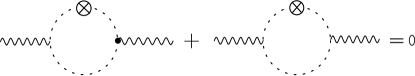
Figure 3: Diagrams which do not contribute to the gluon wave-function renormalization, as they cancel each other. A similar cancellation occurs if one replaces the left vertices of both diagrams with $v$-dependent ones (empty circles).

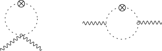
Figure 4: Diagrams which do not contribute to the gluon wave-function renormalization, as they generate a non-quadratic momentum dependence.

The second line in Eq. (105) cannot contribute, as $\Gamma^{(2)}_{M\Phi}$ contains ghost fields. Let’s then address the ghost contributions to the gluon wave-function renormalization, i.e. the term arising from differentiation of the third line in Eq. (105). The second order derivative can be cast in the following form:

$$\frac{\delta\ }{\delta A^{a\mu}}\frac{\delta\ }{\delta A^{b\nu}}\left[\widetilde{\Gamma}^{(2)}_{K^{e}_{\lambda}\Phi^{j}}\big{(}\widetilde{\Gamma}^{(2)-1}\big{)}_{\Phi^{j}(-\bar{c}^{d})}\right]=$$

$$\bigg{\{}\Big{[}\widetilde{\Gamma}^{(3)}_{K^{c}_{\lambda}A^{a\mu}\Phi^{j}}-\widetilde{\Gamma}^{(2)}_{K^{e}_{\lambda}\Phi^{l}}\big{(}\widetilde{\Gamma}^{(2)-1}\big{)}_{\Phi^{l}\Phi^{m}}\widetilde{\Gamma}^{(3)}_{\Phi^{m}A^{a\mu}\Phi^{j}}\Big{]}$$ (160)

$$\phantom{XXXXXX}\times\frac{\delta\ }{\delta A^{b\nu}}\big{(}\widetilde{\Gamma}^{(2)-1}\big{)}_{\Phi^{j}(-\bar{c}^{d})}+\left(\begin{pmatrix}a\\ \mu\end{pmatrix}\leftrightarrow\begin{pmatrix}b\\ \nu\end{pmatrix}\right)\bigg{\}}$$

$$-\widetilde{\Gamma}^{(2)}_{K^{c}_{\lambda}\Phi^{j}}\big{(}\widetilde{\Gamma}^{(2)-1}\big{)}_{\Phi^{j}\Phi^{i}}\widetilde{\Gamma}^{(4)}_{\Phi^{i}A^{a}_{\mu}A^{b}_{\nu}\Phi^{k}}\big{(}\widetilde{\Gamma}^{(2)-1}\big{)}_{\Phi^{k}(-\bar{c}^{d})}.$$

As we must evaluate such derivatives at vanishing fields, all the $\Phi$’s in this expression have to be either ghosts or anti-ghosts. Let us first inspect the $v$-independent contribution. In this case the last line of Eq. (160) vanishes, as the usual Lorenz-gauge ghost action contains no two-ghosts-two-gluons vertex. The remaining terms correspond to the diagrams in Fig. 3. As they carry opposite signs, they sum up to zero. In fact, the $v$-independent terms arising from the square brackets in the second line of Eq. (160), once contracted with $\delta^{ed}$, reduce to $\bar{g}f^{eja}(q^{2}\delta^{\lambda}_{\ \,\mu}-q^{\lambda}q_{\mu})/q^{2}$, where $q$ is the momentum of $K^{a}_{\lambda}(-q)$. As this expression must be contracted with $\partial_{t}(Z_{\mathrm{gh}}r_{\mathrm{gh}}(q^{2}))\mathrm{i}q_{\lambda}$, it drops out of the flow equation.

The $v$-dependent contributions to the gluon wave-function renormalization come in four different forms. Three of them, corresponding to the diagrams in Fig. 4, are vanishing. In fact they show no quadratic term in a Taylor expansion around $p=0$. The only nonvanishing diagram is the second one in Fig. 2. This evaluates to

$$\partial_{t}\Gamma^{(2)}_{A^{a\mu}A^{b\nu}}\Big{|}_{\text{ghost}}=\frac{v^{a}v^{b}}{2Z^{2}|v|^{4}}\int_{q}\frac{{\partial}_{t}R_{\mathrm{gh}}(q^{2})(q+p)^{\alpha}q^{\beta}}{P_{\mathrm{gh}}(q^{2})^{2}P_{\mathrm{gh}}((q+p)^{2})}$$

$$\times\left(R^{\alpha\mu}(p)R^{\beta\nu}(p)+R^{\alpha\mu}(p)R^{\beta\nu}(q)\right.$$ (161)

$$\phantom{\times 1}\left.+R^{\alpha\mu}(q+p)R^{\beta\nu}(p)+R^{\alpha\mu}(q+p)R^{\beta\nu}(q)\right),$$

where

$$R_{\mathrm{gh}}(p^{2}) =p^{2}r_{\mathrm{gh}}(p^{2})\,,$$ (162)

$$P_{\mathrm{gh}}(q^{2}) =q^{2}+R_{\mathrm{gh}}(q^{2})\,.$$ (163)

Therefore

$$\partial_{t}Z_{\mathrm{T}}^{\perp}\Big{|}_{\text{ghost}} =0\,,$$ (164)

$$\partial_{t}Z_{\mathrm{L}}^{\perp}\Big{|}_{\text{ghost}} =0\,.$$ (165)

Notice that Eq. (161) has already been multiplied by a factor 2, to account for the two diagrams with the regulator insertion on different ghost propagators. To extract the ghost-loop contribution to $\partial_{t}Z_{\mathrm{T}/\mathrm{L}}^{\parallel}$ from Eq. (161) we first strip away the factor $\Pi_{\parallel}^{ab}$. We next expand Eq. (161) in a Taylor series about $p=0$ and collect the terms of order $p^{2}$, which can be organized in transverse and longitudinal parts. Finally we adopt the piecewise linear regulator for both the gluon and the ghost sector, as in Eqs. (134) and (135). Setting $p=0$ in the second and third lines of Eq. (161) gives the standard Feynman-gauge result. Expanding these very same terms to second order in $p$ provides the corrections due to the regulator-dependent vertices; see Eqs. (141) and (142), and the subsequent discussion in the main text.

References

- Wetterich (1993) C. Wetterich, Phys. Lett. B301, 90 (1993).
- Bonini et al. (1993) M. Bonini, M. D’Attanasio, and G. Marchesini, Nucl. Phys. B409, 441 (1993), arXiv:hep-th/9301114 [hep-th] .
- Ellwanger (1994a) U. Ellwanger, Proceedings, Workshop on Quantum field theoretical aspects of high energy physics: Bad Frankenhausen, Germany, September 20-24, 1993, Z. Phys. C62, 503 (1994a), [,206(1993)], arXiv:hep-ph/9308260 [hep-ph] .
- Morris (1994) T. R. Morris, Int. J. Mod. Phys. A9, 2411 (1994), arXiv:hep-ph/9308265 [hep-ph] .
- Becchi et al. (1975) C. Becchi, A. Rouet, and R. Stora, Commun. Math. Phys. 42, 127 (1975).
- Becchi et al. (1976) C. Becchi, A. Rouet, and R. Stora, Annals Phys. 98, 287 (1976).
- Tyutin (1975) I. V. Tyutin, (1975), arXiv:0812.0580 [hep-th] .
- Zinn-Justin (1975a) J. Zinn-Justin, Proceedings, International Summer Institute for Theoretical Physics: Trends in Elementary Particle Theory: Bonn, Germany, July 29-August 9, 1974, Lect. Notes Phys. 37, 1 (1975a).
- Zinn-Justin (1975b) J. Zinn-Justin, in Functional and Probabilistic Methods in Quantum Field Theory. 1. Proceedings, 12th Winter School of Theoretical Physics, Karpacz, Feb 17-March 2, 1975 (1975) pp. 433–453.
- Ellwanger (1994b) U. Ellwanger, Phys. Lett. B335, 364 (1994b), arXiv:hep-th/9402077 [hep-th] .
- Bonini et al. (1994) M. Bonini, M. D’Attanasio, and G. Marchesini, Nucl. Phys. B421, 429 (1994), arXiv:hep-th/9312114 [hep-th] .
- D’Attanasio and Morris (1996) M. D’Attanasio and T. R. Morris, Phys. Lett. B378, 213 (1996), arXiv:hep-th/9602156 [hep-th] .
- Litim and Pawlowski (1999) D. F. Litim and J. M. Pawlowski, QCD’98. Proceedings, 3rd Euroconference, 6th Conference, Montpellier, France, July 2-8, 1998, Nucl. Phys. Proc. Suppl. 74, 325 (1999), [,325(1998)], arXiv:hep-th/9809020 [hep-th] .
- Litim and Pawlowski (1998) D. F. Litim and J. M. Pawlowski, in The exact renormalization group. Proceedings, Workshop, Faro, Portugal, September 10-12, 1998 (1998) pp. 168–185, arXiv:hep-th/9901063 [hep-th] .
- Pawlowski (2007) J. M. Pawlowski, Annals Phys. 322, 2831 (2007), arXiv:hep-th/0512261 [hep-th] .
- Gies (2012) H. Gies, ECT* School on Renormalization Group and Effective Field Theory Approaches to Many-Body Systems Trento, Italy, February 27-March 10, 2006, Lect. Notes Phys. 852, 287 (2012), arXiv:hep-ph/0611146 [hep-ph] .
- Ellwanger et al. (1996) U. Ellwanger, M. Hirsch, and A. Weber, Z. Phys. C69, 687 (1996), arXiv:hep-th/9506019 [hep-th] .
- Ellwanger et al. (1998) U. Ellwanger, M. Hirsch, and A. Weber, Eur. Phys. J. C1, 563 (1998), arXiv:hep-ph/9606468 [hep-ph] .
- Gies et al. (2004) H. Gies, J. Jaeckel, and C. Wetterich, Phys. Rev. D69, 105008 (2004), arXiv:hep-ph/0312034 [hep-ph] .
- Fischer and Gies (2004) C. S. Fischer and H. Gies, JHEP 10, 048 (2004), arXiv:hep-ph/0408089 [hep-ph] .
- Fejos and Hatsuda (2017) G. Fejos and T. Hatsuda, Phys. Rev. D96, 056018 (2017), arXiv:1705.07333 [hep-ph] .
- Fischer et al. (2009) C. S. Fischer, A. Maas, and J. M. Pawlowski, Annals Phys. 324, 2408 (2009), arXiv:0810.1987 [hep-ph] .
- Cyrol et al. (2016) A. K. Cyrol, L. Fister, M. Mitter, J. M. Pawlowski, and N. Strodthoff, Phys. Rev. D94, 054005 (2016), arXiv:1605.01856 [hep-ph] .
- Igarashi et al. (2000) Y. Igarashi, K. Itoh, and H. So, Phys. Lett. B479, 336 (2000), arXiv:hep-th/9912262 [hep-th] .
- Sonoda (2007) H. Sonoda, J. Phys. A40, 9675 (2007), arXiv:hep-th/0703167 [HEP-TH] .
- Igarashi et al. (2007) Y. Igarashi, K. Itoh, and H. Sonoda, Prog. Theor. Phys. 118, 121 (2007), arXiv:0704.2349 [hep-th] .
- Igarashi et al. (2016) Y. Igarashi, K. Itoh, and J. M. Pawlowski, J. Phys. A49, 405401 (2016), arXiv:1604.08327 [hep-th] .
- Reuter and Wetterich (1994a) M. Reuter and C. Wetterich, Nucl. Phys. B417, 181 (1994a).
- Reuter and Wetterich (1994b) M. Reuter and C. Wetterich, (1994b), arXiv:hep-th/9411227 [hep-th] .
- Reuter and Wetterich (1997) M. Reuter and C. Wetterich, Phys. Rev. D56, 7893 (1997), arXiv:hep-th/9708051 [hep-th] .
- Freire et al. (2001) F. Freire, D. F. Litim, and J. M. Pawlowski, The exact renormalization group. Proceedings, 2nd Conference, Rome, Italy, September 18-22, 2000, Int. J. Mod. Phys. A16, 2035 (2001), arXiv:hep-th/0101108 [hep-th] .
- Freire et al. (2000) F. Freire, D. F. Litim, and J. M. Pawlowski, Phys. Lett. B495, 256 (2000), arXiv:hep-th/0009110 [hep-th] .
- Bridle et al. (2014) I. H. Bridle, J. A. Dietz, and T. R. Morris, JHEP 03, 093 (2014), arXiv:1312.2846 [hep-th] .
- Becker and Reuter (2014) D. Becker and M. Reuter, Annals Phys. 350, 225 (2014), arXiv:1404.4537 [hep-th] .
- Dietz and Morris (2015) J. A. Dietz and T. R. Morris, JHEP 04, 118 (2015), arXiv:1502.07396 [hep-th] .
- Percacci and Vacca (2017) R. Percacci and G. P. Vacca, Eur. Phys. J. C77, 52 (2017), arXiv:1611.07005 [hep-th] .
- Safari and Vacca (2017) M. Safari and G. P. Vacca, Phys. Rev. D96, 085001 (2017), arXiv:1607.03053 [hep-th] .
- Safari and Vacca (2016) M. Safari and G. P. Vacca, JHEP 11, 139 (2016), arXiv:1607.07074 [hep-th] .
- Gies (2002) H. Gies, Phys. Rev. D66, 025006 (2002), arXiv:hep-th/0202207 [hep-th] .
- Braun et al. (2010) J. Braun, A. Eichhorn, H. Gies, and J. M. Pawlowski, Eur. Phys. J. C70, 689 (2010), arXiv:1007.2619 [hep-ph] .
- Eichhorn et al. (2011) A. Eichhorn, H. Gies, and J. M. Pawlowski, Phys. Rev. D83, 045014 (2011), [Erratum: Phys. Rev.D83,069903(2011)], arXiv:1010.2153 [hep-ph] .
- Morris (1998) T. R. Morris, in The exact renormalization group. Proceedings, Workshop, Faro, Portugal, September 10-12, 1998 (1998) pp. 1–40, arXiv:hep-th/9810104 [hep-th] .
- Arnone et al. (2002) S. Arnone, Y. A. Kubyshin, T. R. Morris, and J. F. Tighe, Int. J. Mod. Phys. A17, 2283 (2002), arXiv:hep-th/0106258 [hep-th] .
- Arnone et al. (2003) S. Arnone, A. Gatti, and T. R. Morris, Phys. Rev. D67, 085003 (2003), arXiv:hep-th/0209162 [hep-th] .
- Arnone et al. (2007) S. Arnone, T. R. Morris, and O. J. Rosten, Eur. Phys. J. C50, 467 (2007), arXiv:hep-th/0507154 [hep-th] .
- Arnone et al. (2004) S. Arnone, A. Gatti, T. R. Morris, and O. J. Rosten, Phys. Rev. D69, 065009 (2004), arXiv:hep-th/0309242 [hep-th] .
- Arnone et al. (2005) S. Arnone, T. R. Morris, and O. J. Rosten, JHEP 10, 115 (2005), arXiv:hep-th/0505169 [hep-th] .
- Morris and Rosten (2006a) T. R. Morris and O. J. Rosten, Phys. Rev. D73, 065003 (2006a), arXiv:hep-th/0508026 [hep-th] .
- Morris and Rosten (2006b) T. R. Morris and O. J. Rosten, J. Phys. A39, 11657 (2006b), arXiv:hep-th/0606189 [hep-th] .
- Evans et al. (2006) N. Evans, T. R. Morris, and O. J. Rosten, Phys. Lett. B635, 148 (2006), arXiv:hep-th/0601114 [hep-th] .
- Rosten (2012) O. J. Rosten, Phys. Rept. 511, 177 (2012), arXiv:1003.1366 [hep-th] .
- Branchina et al. (2003) V. Branchina, K. A. Meissner, and G. Veneziano, Phys. Lett. B574, 319 (2003), arXiv:hep-th/0309234 [hep-th] .
- Pawlowski (2003) J. M. Pawlowski, (2003), arXiv:hep-th/0310018 [hep-th] .
- Donkin and Pawlowski (2012) I. Donkin and J. M. Pawlowski, (2012), arXiv:1203.4207 [hep-th] .
- Wetterich (2016) C. Wetterich, (2016), arXiv:1607.02989 [hep-th] .
- Wetterich (2018) C. Wetterich, Nucl. Phys. B934, 265 (2018), arXiv:1710.02494 [hep-th] .
- Denz et al. (2018) T. Denz, J. M. Pawlowski, and M. Reichert, Eur. Phys. J. C78, 336 (2018), arXiv:1612.07315 [hep-th] .
- Cyrol et al. (2018) A. K. Cyrol, M. Mitter, J. M. Pawlowski, and N. Strodthoff, Phys. Rev. D97, 054006 (2018), arXiv:1706.06326 [hep-ph] .
- Corell et al. (2018) L. Corell, A. K. Cyrol, M. Mitter, J. M. Pawlowski, and N. Strodthoff, (2018), arXiv:1803.10092 [hep-ph] .
- Tissier and Wschebor (2009) M. Tissier and N. Wschebor, (2009), arXiv:0901.3679 [hep-th] .
- Curci and Ferrari (1976a) G. Curci and R. Ferrari, Nuovo Cim. A32, 151 (1976a).
- Curci and Ferrari (1976b) G. Curci and R. Ferrari, Nuovo Cim. A35, 1 (1976b), [Erratum: Nuovo Cim.A47,555(1978)].
- Ojima (1982) I. Ojima, Z. Phys. C13, 173 (1982).
- Delbourgo et al. (1988) R. Delbourgo, S. Twisk, and G. Thompson, Int. J. Mod. Phys. A3, 435 (1988).
- Blasi and Maggiore (1996) A. Blasi and N. Maggiore, Mod. Phys. Lett. A11, 1665 (1996), arXiv:hep-th/9511068 [hep-th] .
- Alkofer and von Smekal (2001) R. Alkofer and L. von Smekal, Phys. Rept. 353, 281 (2001), arXiv:hep-ph/0007355 [hep-ph] .
- Kondo (2001) K.-I. Kondo, Phys. Lett. B514, 335 (2001), arXiv:hep-th/0105299 [hep-th] .
- Ellwanger and Wschebor (2003) U. Ellwanger and N. Wschebor, Int. J. Mod. Phys. A18, 1595 (2003), arXiv:hep-th/0205057 [hep-th] .
- Aguilar et al. (2011) A. C. Aguilar, D. Binosi, and J. Papavassiliou, Phys. Rev. D84, 085026 (2011), arXiv:1107.3968 [hep-ph] .
- Maas (2013) A. Maas, Phys. Rept. 524, 203 (2013), arXiv:1106.3942 [hep-ph] .
- Aguilar et al. (2016) A. C. Aguilar, D. Binosi, and J. Papavassiliou, ECT* Workshop on Dyson-Schwinger Equations in Modern Mathematics and Physics (DSEMP2014) Trento, Italy, September 22-26, 2014, Front. Phys.(Beijing) 11, 111203 (2016), arXiv:1511.08361 [hep-ph] .
- Cucchieri and Mendes (2007) A. Cucchieri and T. Mendes, Proceedings, 25th International Symposium on Lattice field theory (Lattice 2007): Regensburg, Germany, July 30-August 4, 2007, PoS LATTICE2007, 297 (2007), arXiv:0710.0412 [hep-lat] .
- Bogolubsky et al. (2009) I. L. Bogolubsky, E. M. Ilgenfritz, M. Muller-Preussker, and A. Sternbeck, Phys. Lett. B676, 69 (2009), arXiv:0901.0736 [hep-lat] .
- Tissier and Wschebor (2010) M. Tissier and N. Wschebor, Phys. Rev. D82, 101701 (2010), arXiv:1004.1607 [hep-ph] .
- Boucaud et al. (2012) P. Boucaud, J. P. Leroy, A. L. Yaouanc, J. Micheli, O. Pene, and J. Rodriguez-Quintero, Few Body Syst. 53, 387 (2012), arXiv:1109.1936 [hep-ph] .
- Cucchieri et al. (2012) A. Cucchieri, D. Dudal, T. Mendes, and N. Vandersickel, Phys. Rev. D85, 094513 (2012), arXiv:1111.2327 [hep-lat] .
- Tissier and Wschebor (2011) M. Tissier and N. Wschebor, Phys. Rev. D84, 045018 (2011), arXiv:1105.2475 [hep-th] .
- Peláez et al. (2014) M. Peláez, M. Tissier, and N. Wschebor, Phys. Rev. D90, 065031 (2014), arXiv:1407.2005 [hep-th] .
- Reinosa et al. (2014) U. Reinosa, J. Serreau, M. Tissier, and N. Wschebor, Phys. Rev. D89, 105016 (2014), arXiv:1311.6116 [hep-th] .
- Reinosa et al. (2015) U. Reinosa, J. Serreau, M. Tissier, and N. Wschebor, Phys. Lett. B742, 61 (2015), arXiv:1407.6469 [hep-ph] .
- Reinosa et al. (2017) U. Reinosa, J. Serreau, M. Tissier, and N. Wschebor, Phys. Rev. D96, 014005 (2017), arXiv:1703.04041 [hep-th] .
- Berges et al. (2002) J. Berges, N. Tetradis, and C. Wetterich, Phys. Rept. 363, 223 (2002), arXiv:hep-ph/0005122 [hep-ph] .
- Delamotte (2012) B. Delamotte, Lect. Notes Phys. 852, 49 (2012), arXiv:cond-mat/0702365 [cond-mat.stat-mech] .
- Braun (2012) J. Braun, J. Phys. G39, 033001 (2012), arXiv:1108.4449 [hep-ph] .
- Nagy (2014) S. Nagy, Annals Phys. 350, 310 (2014), arXiv:1211.4151 [hep-th] .
- Lavrov and Shapiro (2013) P. M. Lavrov and I. L. Shapiro, JHEP 06, 086 (2013), arXiv:1212.2577 [hep-th] .
- Manrique and Reuter (2009) E. Manrique and M. Reuter, Phys. Rev. D79, 025008 (2009), arXiv:0811.3888 [hep-th] .
- Manrique and Reuter (2011) E. Manrique and M. Reuter, Proceedings, Workshop on Continuum and lattice approaches to quantum gravity (CLAQG08): Brighton, UK, September 17-19, 2008, PoS CLAQG08, 001 (2011), arXiv:0905.4220 [hep-th] .
- Vacca and Zambelli (2011) G. P. Vacca and L. Zambelli, Phys. Rev. D83, 125024 (2011), arXiv:1103.2219 [hep-th] .
- Morris and Slade (2015) T. R. Morris and Z. H. Slade, JHEP 11, 094 (2015), arXiv:1507.08657 [hep-th] .
- Wetterich (1991) C. Wetterich, Nucl. Phys. B352, 529 (1991).
- Kopietz et al. (2010) P. Kopietz, L. Bartosch, and F. Schütz, Lect. Notes Phys. 798, 1 (2010).
- (93) G. P. Vacca and L. Zambelli, In preparation .
- Lippoldt (2018) S. Lippoldt, Phys. Lett. B782, 275 (2018), arXiv:1804.04409 [hep-th] .
- Peskin and Schroeder (1995) M. E. Peskin and D. V. Schroeder, An Introduction to quantum field theory (1995).
- Litim (2001) D. F. Litim, Phys. Rev. D64, 105007 (2001), arXiv:hep-th/0103195 [hep-th] .