New limits on Anomalous Spin-Spin Interactions

Abstract

We report the results of a new search for long range spin-dependent interactions using a Rb -²¹Ne atomic comagnetometer and a rotatable electron spin source based on a SmCo₅ magnet with an iron flux return. By looking for signal correlations with the orientation of the spin source we set new constrains on the product of the pseudoscalar electron and neutron couplings $g^{e}_{p}g^{n}_{p}/\hbar c<1.7\times 10^{-14}$ and on the product of their axial couplings $g^{e}_{A}g^{n}_{A}/\hbar c<5\times 10^{-42}$ to a new particle with a mass of less than about $1~{}\mu$eV. Our measurements improve by about 2 orders of magnitude previous constraints on such spin-dependent interactions.

Long range interactions between spin-polarized objects are dominated by photon-mediated magnetic forces. Additional long range forces may exist if there are new light or massless particles beyond the Standard Model. For example, such new forces arise from exchange of pseudoscalar axions or axion-like particles  Moody and Wilczek (1984), from spin-1 paraphotons or light $Z^{\prime}$ bosons  Dobrescu and Mocioiu (2006); Safronova et al. (2018); from exchange of “unparticles” Georgi (2007); Liao and Liu (2007), dynamical breaking of local Lorentz invariance Arkani-Hamed et al. (2005), or propagating torsion in modified gravity Hammond (1995); Neville (1982). In many of these models significant long-range interactions appear only when both objects are spin-polarized, for example for axion-like particles without a $\bar{\theta}$ term Moody and Wilczek (1984), or for paraphotons– massless gauge boson with dimension-6 operator coupling to fermions Dobrescu and Mocioiu (2006). Overall, search for axion or axion-like particle is of particular interest since they are candidates to explain the unexpected small level of CP violation in QCD or the nature of dark matter.

Experimental searches for anomalous spin-spin interactions were first discussed by Ramsey Ramsey (1979) and have been performed using a variety of systems, including atomic comagnetometers Aleksandrov et al. (1983); Vasilakis et al. (2009), trapped ions Wineland et al. (1991); Kotler et al. (2015), spin-polarized pendulums Heckel et al. (2013); Terrano et al. (2015), polarized geoelectrons Hunter et al. (2013), and NMR spectroscopy Ansel’man and Neronov (1985); Ledbetter et al. (2013). Such experiments typically use a “spin source”– a large collection of spin-polarized fermions and a “spin sensor”– a sensitive system for measurement of the resulting shifts in spin energy levels. Nuclear spin sensors typically have good energy resolution due to long spin coherence times of nuclear spin ensembles. Therefore, it is natural to combine a nuclear spin detector, similar to the one used Vasilakis et al. (2009), with a permanent magnet spin source that provides the highest density of polarized electron spins, as used in Heckel et al. (2013); Terrano et al. (2015).

Here we describe such an experiment searching for electron-nuclear spin-dependent forces using a rotatable SmCo₅ spin source Heckel et al. (2006) and a ²¹Ne-Rb comagnetometer Smiciklas et al. (2011). SmCo₅ has a unique property that part of its magnetization is created by angular moment of the electrons, instead of their spins. This allows one to cancel the net magnetic field created by the spin source without canceling an anomalous spin-dependent force. Our experimental arrangement is sensitive to two spin-dependent potentials in the notation of Dobrescu and Mocioiu (2006) given by:

$$V_{2}= \frac{g^{1}_{A}g^{2}_{A}}{4\pi}\frac{(\hat{\sigma}_{1}.\hat{\sigma}_{2})}{r}e^{-r/\lambda}$$ (1)

$$V_{3}= \frac{g^{1}_{p}g^{2}_{p}\hbar^{2}}{16\pi M_{1}M_{2}c^{2}}\bigg{[}(\hat{\sigma}_{1}.\hat{\sigma}_{2})\big{(}\frac{1}{\lambda r^{2}}+\frac{1}{r^{3}}\big{)}-$$ (2)

$$(\hat{\sigma}_{1}.\hat{r})(\hat{\sigma}_{2}.\hat{r})\big{(}\frac{1}{\lambda^{2}r}+\frac{3}{\lambda r^{2}}+\frac{3}{r^{3}}\big{)}\bigg{]}e^{-r/\lambda}$$

In the above equations, $\hat{\sigma}_{i}$ is the normalized expectation value of the $i^{\rm th}$ particle spin and $M_{i}$ is its mass, $\lambda=\hbar/mc$ is the Yukawa range of the new particle with mass $m$ mediating the spin-dependent force, and $r$ is the distance between the two spins. We set new limits on the product of electron and neutron pseudoscalar coupling constants $g^{e}_{p}g^{n}_{p}$ for $V_{3}$ and the product of the axial vector coupling constants $g^{e}_{A}g^{n}_{A}$ for $V_{2}$. The interaction potential $V_{3}$ can also be generated by a vector particle, such as a paraphoton or $Z^{\prime}$ boson. Our measurements set new limits on the combinations of their parameters described Dobrescu and Mocioiu (2006). One can also set limits in the product of electron and proton spin couplings using the sub-leading proton spin polarization in ²¹Ne Brown et al. (2017). Our limits are substantially better than can be extracted by combining the results of previous electron-electron and nuclear-nuclear spin force experiments.

The Rb-²¹Ne comagnetometer used in this experiment is similar to the one in Smiciklas et al. (2011). More detailed explanation of an its operation can be found in Smiciklas et al. (2011); Brown et al. (2010); Kornack et al. (2005); Brown (2011). At the heart of the comagnetometer is an aluminosilicate GE180 spherical glass-blown cell $1\,$cm in diameter containing $1.5$ amagats of ²¹Ne, $50$ Torr of N₂ (to prevent radiation trapping), ⁸⁷Rb and trace amounts of Cs. The cell is heated up to $180\,^{\circ}$C to create a dense, optically thick vapor of ⁸⁷Rb. The Cs vapor remains optically thin and is optically pumped to create a relatively uniform spin polarization, which is transferred by spin-exchange collisions to Rb and then to ²¹Ne Romalis (2010). Cs is optically pumped using 450 mW of circularly polarized light at 895 nm.

The spin polarization of ⁸⁷Rb is measured via Faraday rotation of a linearly polarized probe beam detuned from $795\,$nm and propagating through the cell in the $\hat{x}$ direction. To measure small optical rotation the linear polarization of the probe beam is modulated at $50\,$kHz by a photoelastic modulator (PEM) and readout using a lock-in amplifier. Low frequency noise from air currents is greatly reduced by operating the experiment inside a vacuum bell jar at pressure of about $1\,$Torr. The probe and pump beams are steered to illuminate the center of the cell, which reduces any spurious effects due to the linear dichroism of the cell walls Kornack (2005).

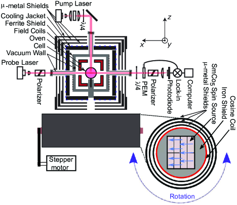
Figure 1: The experimental setup, adapted from Brown et al. (2010). The spin source is placed under the comagnetometer cell with the rotation axis parallel to the probe beam.

The comagnetometer is operated at a compensation point where the external $B_{z}$ field is equal and opposite to the sum of the effective magnetic fields created due to spin-exchange collisions with polarized ⁸⁷Rb and ²¹Ne Kornack (2005). Automated zeroing routines are used to adjust the magnetic fields inside the shields in the $x$, $y$ and $z$ directions. After field zeroing the leading term in the comagnetometer’s signal at the compensation point is:

$$S=\kappa\frac{\gamma_{e}P^{e}_{z}}{R_{tot}}\bigg{[}b_{y}^{n}-b^{e}_{y}+\frac{\Omega_{y}}{\gamma_{n}}\bigg{]},$$ (3)

where $\gamma_{e}$ and $\gamma_{n}$ are the gyromagnetic ratios of the free electron and ²¹Ne, respectively, $P^{e}_{z}$ is the polarization of ⁸⁷Rb, $R_{tot}$ is the total relaxation rate of ⁸⁷Rb, and $b^{n,e}_{y}$ are the anomalous magnetic fields that couple to the ²¹Ne and ⁸⁷Rb electron spins in the $y$ direction. $\Omega_{y}$ is the gyroscopic rotation around the y-axis. The comagnetometer has suppressed sensitivity to ordinary magnetic fields but retains leading order sensitivity to anomalous fields. To calibrate the comagnetometer we measure the response to a slowly modulated $B_{x}$ field  Brown (2011). We verify the calibration factor by measuring the gyroscopic signal due to a slowly changing tilt of the optical table and compare it to the response of the tilt sensors.

The spin source is made from multiple rectangular blocks of SmCo₅ permanent magnet with $7.6\times 7.6\times 20.3\,$cm³ total volume surrounded by a cylindrical soft iron flux return with an outer diameter of 15.2 cm and length of 22.9 cm. The axis of the spin source is 25 cm away from the center of the comagnetometer cell. The remnant magnetic field outside of the iron cylinder is about $0.6\,$ mT, in good agreement with finite element magnetic field analysis. To further reduce this field, a cosine coil is mounted on the outside of the iron cylinder and three layers of $\mu$-metal shields are added around the spin source. The coil allows us to cancel the residual leakage of the fields by a factor of 10 or alternatively increase the field to check for systematic sensitivity of the comagnetometer. The orientation of the spin source is reversed by rotating the cylinder around its axis using a stepper motor and a timing belt while keeping the outer two magnetic shield layers fixed. The residual magnetic field correlated to the orientation of the spin source is equal to approximately $2.5\times 10^{-9}\,$T. The comagnetometer apparatus is vibrationally isolated from the mechanical rotation system inside the vacuum bell jar.

Fully magnetized SmCo₅ with $B_{0}\approx 1$ T has an electron spin density of $4.5\times\,10^{22}\,\text{spin}/\text{cm}^{3}$ while soft iron with the same magnetization has a spin density of $8.2\times\,10^{22}\,\text{spin}/\text{cm}^{3}$  Heckel et al. (2008); Ji et al. (2017). Hence the spin source posses a large net electron spin while having only a small residual magnetic dipole moment. The presence of net spin in a similar structure had been verified in Heckel et al. (2008) by observing the gyrocompass signal. The use of magnetic shielding does not screen anomalous spin interactions. Magnetic shielding around the spin source has a similar spin content to the soft-iron flux return. The magnetic shielding around the comagnetometer cannot hide the signal, as discussed in Kimball et al. (2016), because we compare spin interactions of electron and nuclear spins in the ⁸⁷Rb-Ne comagnetometer. The rotation of the spin source is controlled by a separate computer to minimize possible cross-talk with the main system operating the experiment.

Data is collected in intervals of $250\,$s during which the spin source is rotated by 180^∘ 19 times every 12 seconds. String analysis Kornack (2005) is used to calculate the correlation of the comagnetometer signal with spin source orientation, using only the last 2 seconds to allow the system to settle mechanically after each rotation. The $B_{z}$ field is adjusted at the end of each interval, while the other field components are zeroed and the comagnetometer sensitivity is calibrated every seven hours.

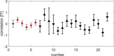
Figure 2: Measured correlation for positive polarization (red), negative polarization (black), clockwise spin source rotation (triangles pointing down), counterclockwise ones (triangles pointing up).

Type	Weighted averaged correlation (aT)	Reduced $\chi^{2}$
$b^{y}_{p-}$	$-180\pm 110$	1.53
$b^{y}_{p+}$	$-9\pm 83$	0.743
$b^{y}_{ccw}$	$-71\pm 89$	1.07
$b^{y}_{cw}$	$-140\pm 140$	1.97
$b^{y}_{tot}$	$-80\pm 70$	1.32

Table 1: Measured correlation for negative polarization ($b^{y}_{p-}$), positive polarization ($b^{y}_{p+}$), counter clockwise spin source rotation ($b^{y}_{ccw}$), clockwise spin source rotation ($b^{y}_{cw}$), and total correlation ($b^{y}_{tot}$).

Sensors	Averaged correlation (aT)
Fluxgate X	$-41\pm 1$
Fluxgate Y	$48\pm 1$
Fluxgate Z	$-52\pm 1$
Probe Beam Position (H)	$-14\pm 38$
Probe Beam Position (V)	$12\pm 11$
Probe Beam Power	$8\pm 10$
Pump Beam Position (H)	$-6.1\pm 16$
Pump Beam Position (V)	$91\pm 138$
Pump Beam Power	$-31\pm 26$
Tilt Rate Y ($\Omega_{y}$)	$-110\pm 82$
Tilt Rate X ($\Omega_{x}$)	$-1.4\pm 9$
Total	$-96\pm 169$

Table 2: Signal correlation estimated from external sensors.

Figure 2 shows the results of approximately two weeks of data. Each data point corresponds to a $\sim 24$ hours measurement. We collected data with clockwise and counter-clockwise spin source rotations and for two orientations of the atomic spin polarization. The results of the measurements of $b_{y}^{n}-b^{e}_{y}$ are summarized in Table 1. The error bars are scaled by the value of reduced $\chi^{2}$. Extended discussion about the method used to obtain uncertainty and reduced $\chi^{2}$ can be found in Brown (2011); Lee (2019).

To check for possible systematic effects correlated with spin source orientation we monitor the magnetic fields, tilts of the comagnetometer platform, positions of the laser beams, as well as other signals that did not show significant effects. Measurements of the magnetic fields at several positions around the apparatus with a fluxgate magnetometer have average correlated field amplitudes of $8.2\times 10^{-10}\,$T, $2.4\times 10^{-9}\,$T and $2.6\times 10^{-10}\,$T for $\hat{x}$, $\hat{y}$ and $\hat{z}$ directions, respectively. The combination of magnetic shielding around the cell and the comagnetometer compensation give an additional suppression of external fields by $5\times 10^{-8}$ for $\hat{x}$ and higher suppressions for $\hat{y}$ and $\hat{z}$ axes. Two 4-quadrant photodiodes monitor the positions and powers of the pump and probe beams. A separate set of measurements was used to find the correlation between the rotation of the spin source and the beams’ positions for both clockwise and counterclockwise rotations of the spin source in the same analysis window as the main measurement. To estimate sensitivity to beam motion, larger beam motion was induced while monitoring the comagnetometer signal. A precision tiltmeter mounted on the same vibration-isolation platform as the comagnetometer measured the residual rotation rate of the platform correlated with spin source reversal.

Tab. 2 shows the summary of measured systematic effects. The total systematic error from magnetic field leakages, beam positions and power, as well as gyroscopic couplings is constrained with an uncertainty of $169\,$aT. Our assumption is that systematic effects recorded for the relevant sensor correlations are independent. Hence, we can combine their uncertainties in quadrature to provide an estimate of the overall systematic uncertainty. Hence, we quote the final total anomalous coupling as $b^{y}_{tot}=-80\pm 70_{stat}\pm 169_{syst}$. This yields, at the $95\%$ confidence level, $|b^{y}_{tot}|<400$ aT.

To convert the measured value of $b^{y}_{n}-b^{y}_{e}$ to limits on spin-spin interactions we express the energy shift due to the anomalous potentials for neutrons, protons and electrons as $V_{n}f_{n}+V_{p}f_{p}-V_{e}=\mu_{{}^{21}Ne}b^{n}_{y}-\mu_{B}\beta^{e}_{y}$, where $f_{n}=0.58$ and $f_{p}=0.04$ are the fraction of neutron and proton spin polarization in ²¹Ne Brown et al. (2017). The interactions given by Eq. (1,2) are integrated over the distribution of the polarized spins in the SmCo₅ magnets and the soft-iron flux return.

The limits on the pseudoscalar and axial coupling constants are summarized in Table 3 and Figs. 3, 4. Only one prior experiment has constrained directly the $g^{n}_{p}g^{e}_{p}$ combination Wineland et al. (1991). More stringent limits can be obtained by combining the limit on $(g^{e}_{p})^{2}$ from Terrano et al. (2015) and the limit on $(g^{n}_{p})^{2}$ from Vasilakis et al. (2009). If the pseudoscalar particle is coupled to fermions through a Yukawa interaction (as opposed to the derivative coupling typical for axions), one can also obtain a limit on $(g^{n}_{p})^{2}$ from two-particle exchange using equivalence principle experiments Fischbach and Krause (1999). Several additional limits can be set on combinations of coupling parameters for paraphoton and $Z^{\prime}$ boson from the expressions for $V^{en}_{3}$ derived in Dobrescu and Mocioiu (2006). We also set limits on the product of axial couplings $g^{n}_{A}g^{e}_{A}$ for a vector boson exchange, improving on previous direct Hunter et al. (2013) and indirect limits Heckel et al. (2013); Vasilakis et al. (2009) for a particle with Yukawa range of $1$ cm to $10^{6}$ cm. Several additional constraints on the order of $10^{-10}-10^{-18}$ exist for $(g_{A})^{2}/\hbar c$ that extend to much shorter length scales Ledbetter et al. (2013); Kotler et al. (2015); Ficek et al. (2018).

Coupling	This work	Previous limit	Reference
$g^{e}_{p}g^{n}_{p}/\hbar c$	$1.7\times 10^{-14}$	$8.1\times 10^{-12}$	Direct: Wineland et al. (1991)
		$9.0\times 10^{-13}$	$(g^{e}_{p})^{2}(g^{n}_{p})^{2}:$ Terrano et al. (2015); Vasilakis et al. (2009)
		$5.9\times 10^{-12}$	Only for Yukawa
			coupling:  Terrano et al. (2015); Adelberger et al. (2007)
$g^{e}_{p}g^{e}_{p}/\hbar c$	$1.5\times 10^{-14}$	$5.5\times 10^{-17}$	Direct: Terrano et al. (2015)
$g^{e}_{A}g^{n}_{A}/\hbar c$	$5.0\times 10^{-42}$	$4.8\times 10^{-40}$	$(g^{e}_{A})^{2}(g^{n}_{A})^{2}$: Heckel et al. (2013); Vasilakis et al. (2009)
$g^{e}_{A}g^{e}_{A}/\hbar c$	$8.0\times 10^{-39}$	$7.6\times 10^{-40}$	Direct: Heckel et al. (2013)

Table 3: Experimental limits (95% CL) on anomalous spin-spin interaction between two fermions by spin-$0$ or spin-$1$ boson exchange with Yukawa range of $10^{2}$ to $10^{6}$ cm.

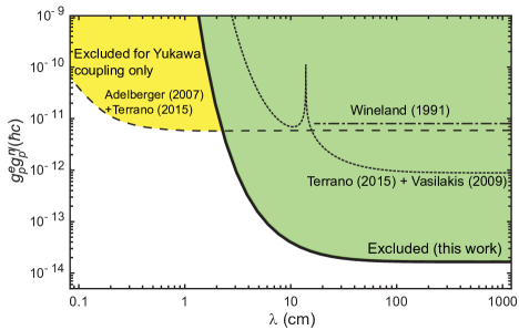
Figure 3: Constraints ($95\%$ CL) on the coupling parameter $g^{n}_{p}g^{e}_{p}$ for two fermions interacting by a pseudoscalar boson.

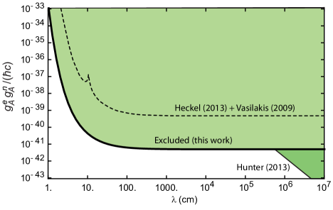
Figure 4: Constraints ($95\%$ CL) on the coupling parameters $g^{n}_{A}g^{e}_{A}$ for two fermions interacting by a spin-1 boson.

In conclusion, we have improved limits on spin-dependent interactions between electrons and neutrons mediated by a new light pseudoscalar or vector boson by about 2 orders of magnitude. The experimental uncertainties are dominated by mechanical transients which produce the largest systematic errors and force us to use a short integration time and a slow source reversal. The sensitivity can be improved by about 2 orders of magnitude with a better vibration isolation system to reduce the motion associated with the mechanical reversal of the spin source. We like to thank Justin Brown, Lawrence Cheuk, David Hoyos, and Ahmed Akhtar for assistance in the design and assembly of the spin source. This work was supported by NSF Grant No. 1404325.

References

- Moody and Wilczek (1984) J. E. Moody and F. Wilczek, Phys. Rev. D 30, 130 (1984).
- Dobrescu and Mocioiu (2006) B. A. Dobrescu and I. Mocioiu, J. High Energy Phys. 2006, 5 (2006).
- Safronova et al. (2018) M. Safronova, D. Budker, D. DeMille, D. F. J. Kimball, A. Derevianko, and C. W. Clark, Reviews of Modern Physics 90, 025008 (2018).
- Georgi (2007) H. Georgi, Phys. Rev. Lett. 98, 221601 (2007).
- Liao and Liu (2007) Y. Liao and J.-Y. Liu, Phys. Rev. Lett. 99, 191804 (2007).
- Arkani-Hamed et al. (2005) N. Arkani-Hamed, H.-C. Cheng, M. Luty, and J. Thaler, J. High Energy Phys. 2005, 29 (2005).
- Hammond (1995) R. T. Hammond, Phys. Rev. D 52, 6918 (1995).
- Neville (1982) D. E. Neville, Phys. Rev. D 25, 573 (1982).
- Ramsey (1979) N. F. Ramsey, Physica A 96, 285 (1979).
- Aleksandrov et al. (1983) E. B. Aleksandrov, A. A. Anselm, Y. V. Pavlov, and R. M. Umarkhodjaev, Zh. Eksp. Teor. Fiz 85, 1899 (1983).
- Vasilakis et al. (2009) G. Vasilakis, J. M. Brown, T. W. Kornack, and M. V. Romalis, Phys. Rev. Lett. 103, 261801 (2009).
- Wineland et al. (1991) D. J. Wineland, J. J. Bollinger, D. J. Heinzen, W. M. Itano, and M. G. Raizen, Phys. Rev. Lett. 67, 1735 (1991).
- Kotler et al. (2015) S. Kotler, R. Ozeri, and D. F. Jackson-Kimball, Phys. Rev. Lett. 115, 081801 (2015).
- Heckel et al. (2013) B. R. Heckel, W. A. Terrano, and E. G. Adelberger, Phys. Rev. Lett. 111, 151802 (2013).
- Terrano et al. (2015) W. A. Terrano, E. G. Adelberger, J. G. Lee, and B. R. Heckel, Phys. Revl. Lett. 115, 201801 (2015).
- Hunter et al. (2013) L. Hunter, J. Gordon, S. Peck, D. Ang, and J.-F. Lin, Science 339, 928 (2013).
- Ansel’man and Neronov (1985) A. A. Ansel’man and Y. I. Neronov, Zh. Eksp. Teor. Fiz. 88, 1946 (1985).
- Ledbetter et al. (2013) M. P. Ledbetter, M. V. Romalis, and D. F. Jackson-Kimball, Phys. Rev. Lett. 110, 040402 (2013).
- Heckel et al. (2006) B. R. Heckel, C. E. Cramer, T. S. Cook, E. G. Adelberger, S. Schlamminger, and U. Schmidt, Phys. Rev. Lett. 97, 021603 (2006).
- Smiciklas et al. (2011) M. Smiciklas, J. M. Brown, L. W. Cheuk, S. J. Smullin, and M. V. Romalis, Phys. Rev. Lett. 107, 171604 (2011).
- Brown et al. (2017) B. A. Brown, G. F. Bertsch, L. M. Robledo, M. V. Romalis, and V. Zelevinsky, 119, 192504 (2017).
- Brown et al. (2010) J. M. Brown, S. J. Smullin, T. W. Kornack, and M. V. Romalis, Phys. Rev. Lett. 105, 151604 (2010).
- Kornack et al. (2005) T. W. Kornack, R. K. Ghosh, and M. V. Romalis, Phys. Rev. Lett. 95, 230801 (2005).
- Brown (2011) J. M. Brown, Ph.D. thesis, Princeton University (2011).
- Romalis (2010) M. V. Romalis, Phys. Rev. Lett. 105, 243001 (2010).
- Kornack (2005) T. W. Kornack, Ph.D. thesis, Princeton University (2005).
- Heckel et al. (2008) B. R. Heckel, E. G. Adelberger, C. E. Cramer, T. S. Cook, S. Schlamminger, and U. Schmidt, Phys. Rev. D 78, 092006 (2008).
- Ji et al. (2017) W. Ji, C. B. Fu, and H. Gao, Physical Review D 95, 075014 (2017).
- Kimball et al. (2016) D. F. Jackson-Kimball, J. Dudley, Y. Li, S. Thulasi, S. Pustelny, D. Budker, and M. Zolotorev, Phys. Rev. D 94, 082005 (2016).
- Lee (2019) J. Lee, Ph.D. thesis, Princeton University (2019).
- Fischbach and Krause (1999) E. Fischbach and D. E. Krause, Phys. Rev. Lett. 82, 4753 (1999).
- Ficek et al. (2018) F. Ficek et al., Phys. Rev. Lett. 120, 183002 (2018).
- Adelberger et al. (2007) E. G. Adelberger, B. R. Heckel, S. Hoedl, C. D. Hoyle, D. J. Kapner, and A. Upadhye, Phys. Rev. Lett. 98, 131104 (2007).