Calculated magnetic exchange interactions in Dirac magnon material Cu₃TeO₆

Abstract

Recently topological aspects of magnon band structure have attracted much interest, and especially, the Dirac magnons in Cu₃TeO₆ have been observed experimentally. In this work, we calculate the magnetic exchange interactions J’s using the first-principles linear-response approach and find that these $J^{\prime}s$ are short-range and negligible for the Cu-Cu atomic pair apart by longer than 7 Å. Moreover there are only 5 sizable magnetic exchange interactions, and according to their signs and strengths, modest magnetic frustration is expected. Based on the obtained magnetic exchange couplings, we successfully reproduce the experimental spin-wave dispersions. The calculated neutron scattering cross section also agrees very well with the experiments. We also calculate Dzyaloshinskii-Moriya interactions (DMIs) and estimate the canting angle ($\sim$ 1.3^∘) of the magnetic non-collinearity based on the competition between DMIs and J’s, which is consistent with the experiment. The small canting angle agrees with that the current experiments cannot distinguish the DMI induced nodal line from a Dirac point in the spin-wave spectrum. Finally we analytically prove that the “sum rule” conjectured in [Nat. Phys. 14, 1011 (2018)] holds but only up to the 11th nearest neighbour.

I Introduction

The non-trivial topological nature of electronic bands has been studied extensively during the past decade Hasan and Kane (2010); Qi and Zhang (2011). Plenty of topological materials have been discovered, such as topological insulator Hasan and Kane (2010); Qi and Zhang (2011), Dirac semimetal Young et al. (2012); Wang et al. (2012, 2013); Gibson et al. (2015); Du et al. (2015); Yang and Nagaosa (2014), Weyl semimetal Wan et al. (2011a); Huang et al. (2015); Weng et al. (2015a) and node-line semimetal Burkov et al. (2011); Weng et al. (2015b); Yu et al. (2015); Kim et al. (2015); Du et al. (2017), etc Bansil et al. (2016). In addition to the above topological phases, the rich variety of spatial symmetries in condensed matter systems results in various novel topological crystalline insulators/semimetals Ando and Fu (2015); Wang et al. (2016); Slager et al. (2013); Langbehn et al. (2017); Song et al. (2017); Benalcazar et al. (2017); Bzd$\check{\mathrm{s}}$ek et al. (2016). By exploiting the mismatch between the real and momentum-space descriptions of the band structure, a complete classification scheme of band topology has been proposed Po et al. (2017); Bradlyn et al. (2017); Kruthoff et al. (2017); Watanabe et al. (2018). A comprehensive database search for ideal non-magnetic topological materials has been finished Tang et al. (2018a) by combining first principles calculation and the symmetry-indicator theory Tang et al. (2018b). Meanwhile, thousands of electronic topological materials have also been proposed based on the graph theory Vergniory et al. (2018) and the complete mapping between the symmetry representation of occupied bands and the topological invariants Zhang et al. (2018).

It is worth mentioning that the topological feature is not only restricted to electronic systems. The band crossings in systems of photons Lu et al. (2014); Zilberberg et al. (2018); Zhou et al. (2018); Yang et al. (2018) and phonons Stenull et al. (2016); Serra-Garcia et al. (2018) have also been intensively investigated. Moreover, recent research in the magnon systems has leaded to the discovery of topological magnon insulators Mook et al. (2014); Zhang et al. (2013), magnonic Dirac semimetals Fransson et al. (2016); Owerre (2017); Pershoguba et al. (2018) and Weyl semimetals Li et al. (2016); Mook et al. (2016); Su et al. (2017).

In 2017, Li et al. Li et al. (2017) proposed Dirac magnons may occur in the three-dimensional antiferromagnetic material Cu₃TeO₆. As shown in Fig. 1, Cu₃TeO₆ crystallizes in the centrosymmetric cubic crystal structure (space group $Ia$-$3$) Hostachy and Coing-Boyat (1968); Falck et al. (1978). Temperature ($T$) dependent magnetic susceptibility ($\chi(T)$) reveals that this compound displays a long-range antiferromagnetic (AFM) ordering below $T$${}_{N}\sim 60\$K Herak et al. (2005). Within the range of $T=180-330$ K, $\chi(T)$ can be fitted very well by the Curie-Weiss (CW) law with the CW temperature $\theta_{CW}=-130$ K Herak et al. (2005). The $\chi(T)$ deviates from CW behavior below 180 K, which is three times larger than $T$_N. This may indicate the frustrated magnetic feature Herak et al. (2005). A clear bulk magnetic transition at around 62 K has also been observed by muon-spin relaxation/rotation measurement Månsson et al. (2012). Neutron powder diffraction experiment Herak et al. (2005) suggests two possible magnetic configurations: (i) collinear AFM order (ii) non-collinear configuration. In the collinear case, the two spins connected by inversion ($\mathcal{P}$) have opposite spin orientations Herak et al. (2005), thus Cu₃TeO₆ is invariant under $\mathcal{P}\mathcal{T}$ symmetry ( $\mathcal{T}$ is the time-reversal transformation), protecting robust magnon Dirac points Li et al. (2017). For the non-collinear magnetic case Herak et al. (2005), Li et al. Li et al. (2017) propose that non-collinearity breaks the U(1) symmetry. As a result, the Dirac point in the collinearly magnetically ordered state expands into a nodal line Li et al. (2017).

Motivated by this theoretical prediction, Yao et al. Yao et al. (2018) and Bao et al. Bao et al. (2018) have measured spin excitations of Cu₃TeO₆ with inelastic neutron scattering (INS), respectively. Both of them have observed the existence of band crossing points in the magnon spectra Yao et al. (2018); Bao et al. (2018). In addition to Dirac points, at $\Gamma$ and $H$ points of the Brillouin zone (BZ) Bao et al. Bao et al. (2018) also observed the triply degenerate nodes which can also occur in electronic bands Bradlyn et al. (2016); Lv et al. (2017). Bao et al. Bao et al. (2018) found that the experimental magnon band dispersion can be well reproduced by a spin Hamiltonian dominated by only the 1st nearest-neighbour (NN) exchange interaction J₁. While Yao et al. Yao et al. (2018) suggested that the magnetic moments in this compound couple over a variety of distances, and even the ninth-nearest-neighbour J₉ plays an important role. Strikingly they found an interesting relation between magnon eigenvalues at different high symmetry points of BZ which was dubbed as “sum rule” Yao et al. (2018).

Generally, spin-orbit coupling (SOC) always exists and leads to the Dzyaloshinskii-Moriya interactions (DMIs) Dzyaloshinsky (1958); Moriya (1960) even in the centrosymmetric compound Cu₃TeO₆, as discussed in the following sections. The DMIs could result in a non-collinearity in the ground magnetic state, leading to nodal lines in magnetic excitations Li et al. (2017). As mentioned above, the two experiments Yao et al. (2018); Bao et al. (2018) have observed the existence of Dirac points but cannot identify the nodal lines from the band crossing points. Note that the size of nodal lines strongly depends on the canting angle of the non-collinearity, which is determined by the competition between exchange interaction $J$ and DMI Li et al. (2017). Therefore it is an interesting issue to obtain accurate spin exchange parameters $J^{\prime}s$ and DMIs, which we address in the current work.

In this paper, based on first-principles calculations, we systematically study the electronic and magnetic properties of Cu₃TeO₆. The calculations show that Cu₃TeO₆ is an insulator with a band gap about 2.07 eV. The calculated magnetic moment of Cu ions is about 0.81 $\mu_{B}$, which is larger than the experimental value (0.64 $\mu_{B}$) measured by the neutron powder diffraction Herak et al. (2005). Using a first-principles linear-response (FPLR) approach Wan et al. (2006), we calculate the spin exchange parameters $J^{\prime}s$. Based on these spin exchange parameters, we calculate the magnetic excitation spectra using linear spin wave theory (LSWT) and the calculated spin wave spectra agree with the experiments very well, as well as the positions of the Dirac and triply degenerate magnons in the BZ Yao et al. (2018); Bao et al. (2018). We also calculate the neutron scattering cross section, which is consistent with the experiment Yao et al. (2018); Bao et al. (2018). The calculated exchange interactions are short-range and negligibly weak for the distance more than 7 Å. There are only five sizable magnetic exchange terms and all them favor antiferromagnetic ordering. These spin exchange parameters are compatible with the modest frustration in Cu₃TeO₆ according to their signs and magnitudes. We also analytically prove that the magnon energies at high symmetry points of BZ cannot own a general “sum rule” conjectured in Ref. Yao et al. (2018) which is found to be only satisfied up to the 11th NN. Moreover, we also calculate the DMIs and estimate the canting angle of non-collinearity which is about 1.3^∘, consistent with the experimental value $\sim$ 6^∘ Herak et al. (2005). This may be the reason why the recent experimental works only observed the existence of Dirac points instead of the nodal lines Yao et al. (2018); Bao et al. (2018).

II Method

The electronic band structure and density of states calculations are carried out by using the full potential linearized augmented plane wave method as implemented in WIEN2K package Blaha et al. (2001). Local spin density approximation (LSDA) for the exchange-correlation potential is used here. A 10$\times$10$\times$10 k-point mesh is used for the Brillouin zone integral. Using the second-order variational procedure, we include the SOC interaction Koelling and Harmon (1977). The self-consistent calculations are considered to be converged when the difference of the total energy of the crystal does not exceed 0.01 mRy. We utilize the LSDA + $U$ scheme Anisimov et al. (1997) to take into account the effect of Coulomb repulsion in Cu-$3d$ orbital. The value of $U=10$ eV and $J=1$ eV for Cu-oxides works well in the previous theoretical work Anisimov et al. (2002); Wan et al. (2009). We vary the parameter $U$ between 8.0 and 10.0 eV and find that our results are not sensitive to the values of $U$ in this range. Thus in this paper we show our results for $U=10$ eV.

The spin exchange parameters $J^{\prime}s$ are the basis to understand magnetic properties. By fitting $J$ to reproduce experimental results, such as $\chi(T)$ and magnon dispersion, one can extract the exchange interaction parameters $J^{\prime}s$Ḣowever, an unambiguous fitting is basically impossible. For example, as mentioned above, though the INS experimental results of Yao et al. and Bao et al. are consistent with each other, their fitting results of the spin exchange interactions are completely different Yao et al. (2018); Bao et al. (2018). In addition to this phenomenological approach, theoretical calculations can also be used to estimate the exchange interaction parameters. A popular numerical method to calculate $J$ is to calculate the total energies of the $N+1$ magnetic configurations, and map it by a spin Hamiltonian to extract $N$ exchange constants. Unfortunately this theoretical method has several drawbacks: (i) the calculated magnetic moments may depend on the magnetic ordering, which significantly affect the accuracy of the obtained J; (ii) it is not clear that how many exchange interactions J one need to use when mapping the total energies from the first-principles calculation on the spin Hamiltonian. An alternative but much more efficient method to calculate spin exchange interactions by first-principles is based on combining magnetic force theorem and linear-response approach Liechtenstein et al. (1987). The exchange interaction parameters are determined via calculation of second variation of total energy for small deviation of magnetic moments Liechtenstein et al. (1987). This method allows one to calculate $J(\mathbf{q})$, the lattice Fourier transform of the exchange interactions $J(\mathbf{R}_{l})$. Thus one can easily calculate long-range exchange interactions accurately even in complicated systems like Cu₃TeO₆ here owing a highly-interconnected three-dimensional spin network. Recently this technique has been used successfully for evaluating magnetic interactions including DMIs in a series of materials Wan et al. (2006); Liechtenstein et al. (1987); Frota-Pessôa et al. (2000); Pajda et al. (2001); Fischer et al. (2009); Galanakis and Şaşıoğlu (2012); Wan et al. (2009); Mazurenko and Anisimov (2005); Katsnelson et al. (2010); Wan et al. (2011b), and is employed in this work to estimate the spin exchange parameters $J^{\prime}s$ and DMIs Wan et al. (2006).

III Results

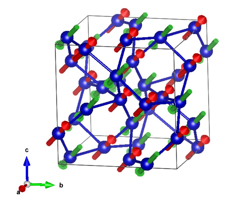
Figure 1: Crystal structure of Cu₃TeO₆ Hostachy and Coing-Boyat (1968); Falck et al. (1978). Only Cu ions are shown for simplicity. We refer to the spins as red and green arrows along [111] direction.

As shown in Fig. 1, Cu₃TeO₆ crystallizes in the centrosymmetric spin-web compound. The highly-interconnected three-dimensional spin network consists of 12 Cu ions per primitive cell, where six Cu ions form an almost coplanar hexagon and each Cu ion is shared by two hexagons. Based on the collinear antiferromagnetic configuration suggested by neutron powder diffraction experiment Herak et al. (2005) as shown in Fig. 1, we perform the first-principles calculations. Here we adopt the LSDA + $U$ (= 10 eV) scheme, which is adequate for the magnetically ordered insulating states Kotliar et al. (2006). The band structures and the density of states are shown in Fig. 2 and Fig. 3, respectively. Our calculations indicate that Cu₃TeO₆ is an insulator with a band gap about 2.07 eV from LSDA + $U$ (= 10 eV) calculations. The O-$2p$ states are mainly located between $-$8.0 and 0.0 eV, while Te $5s$ and $5p$ bands appear mainly above 3.0 eV. Hence the nominal valence for Te is $+6$ while that for O is $-2$. As a result, Cu ions have the nominal valence of +2, indicating the $3d^{9}$ electronic configuration. The nine $3d$ occupied states of Cu ions are mainly located from $-$8.0 to $-$3.0 eV, implying strong hybridization between Cu and O states. Meanwhile the only one unoccupied state of Cu²⁺ ions appears mainly between 3.0 to 5.0 eV. Despite of strong hybridization between Cu and O states, the calculated magnetic moment at the O site is negligible ($\sim$ 0.01 $\mu_{B}$), and the major magnetic moment is located at the Cu site. The calculated magnetic moment of the Cu ions is 0.81 $\mu_{B}$, which is smaller than the ideal $3d^{9}$ ($S$= $1/2$) configuration and larger than the experimental value 0.64 $\mu_{B}$ Herak et al. (2005).

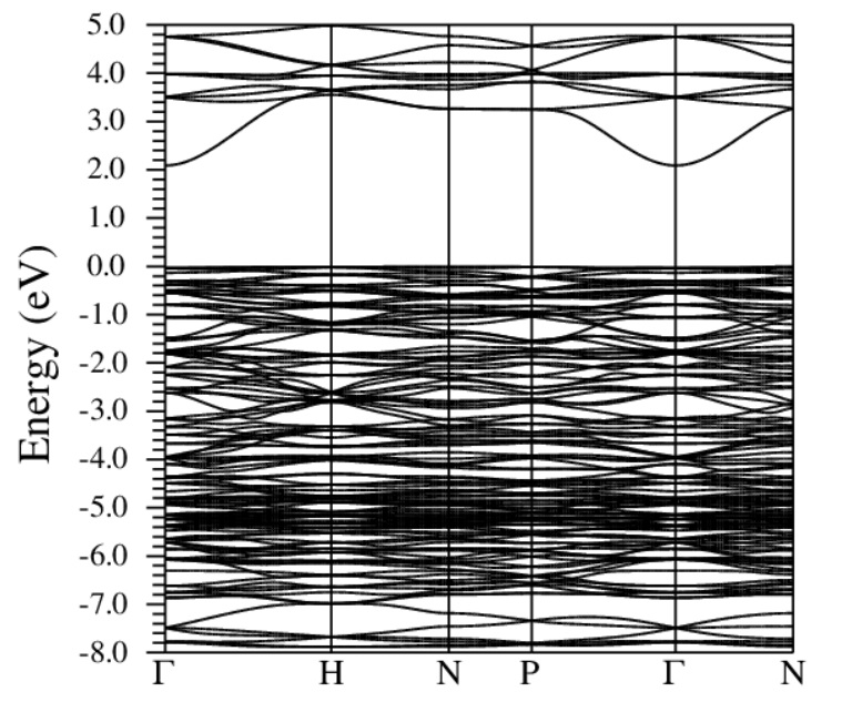
Figure 2: Band structures of Cu₃TeO₆ from LSDA + $U$ (= 10 eV) calculation with antiferromagnetic configuration. The Fermi energy is set to zero.

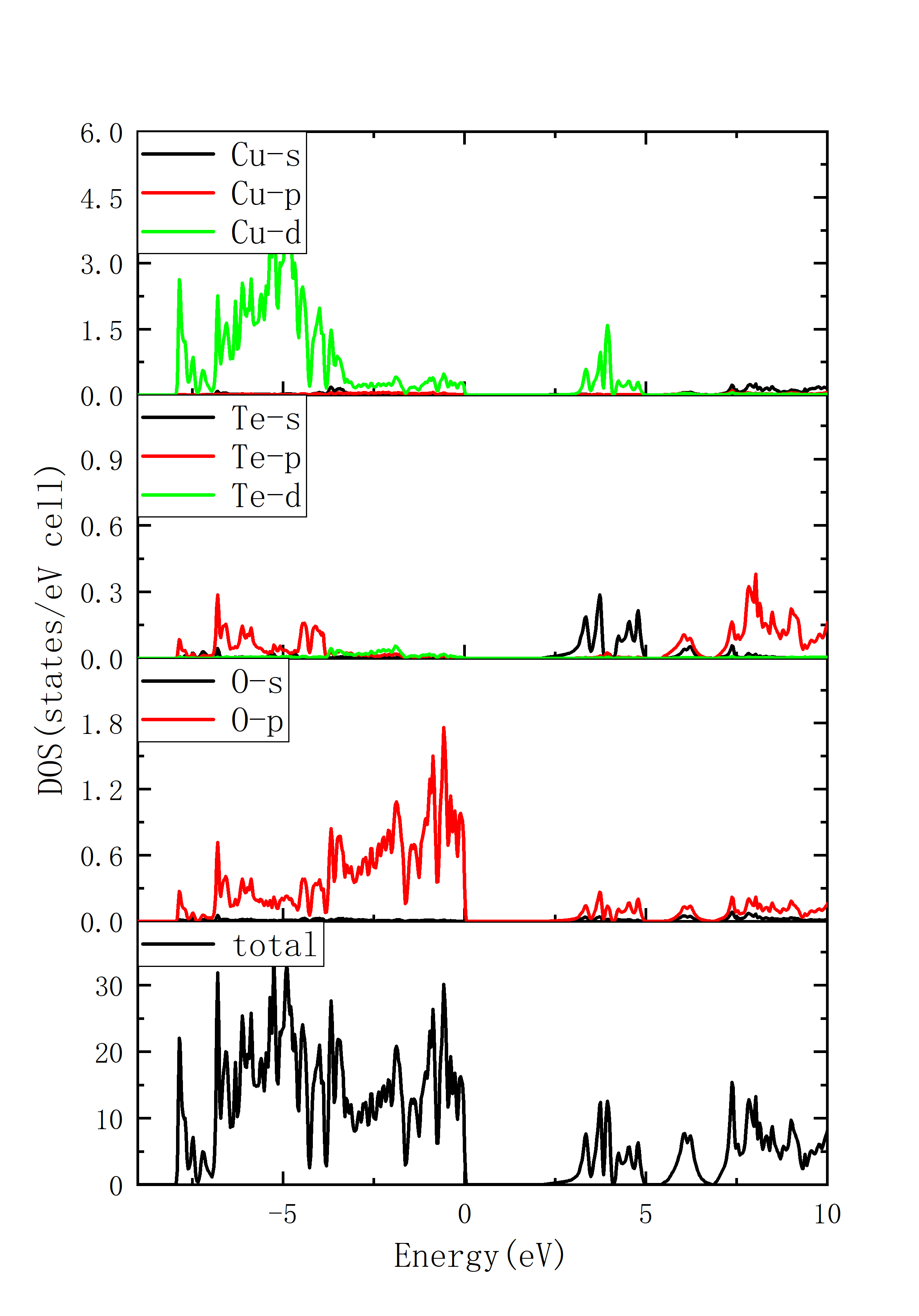
Figure 3: Partial density of states (PDOS) of Cu₃TeO₆ from LSDA + $U$ (= 10 eV) calculation. The Fermi energy is set to zero.

Table 1: Calculated spin exchange parameters (in meV) evaluated from LSDA + $U$ (= 10 eV) scheme. The Cu-Cu distances and the corresponding number of neighbours are presented in the 2nd the 3rd columns. The fitting spin exchange parameters in the experimental work are also presented for comparison.

	Distance(Å)	NN	Ref. Bao et al. (2018)	Ref. Yao et al. (2018)	Our results
$J_{1}$	3.18	4	9.07	4.49	7.05
$J_{2}$	3.60	4	0.89	-0.22	0.51
$J_{3}$	4.77	2	-1.81	-1.49	0.04
$J_{4}$	4.81	2	1.91	1.33	2.18
$J_{5}$	4.81	2	1.91	1.79	0.09
$J_{6}$	5.48	4	0.09	-0.21	0.01
$J_{7}$	5.73	4	1.83	-0.14	-0.01
$J_{8}$	5.97	4	–	0.11	0.04
$J_{9}$	6.21	4	–	4.51	3.77
$J_{10}$	6.34	2	–	–	0.56
$J_{11}$	6.34	2	–	–	-0.01
$J_{12}$	6.74	4	–	–	0.02
$J_{13}$	7.17	2	–	–	-0.06
$J_{14}$	7.17	2	–	–	-0.04
$J_{15}$	7.27	4	–	–	0.00
$J_{16}$	7.46	4	–	–	0.02
$J_{17}$	7.64	4	–	–	0.10
$J_{18}$	7.83	4	–	–	0.00
$J_{19}$	8.26	4	–	–	-0.02
$J_{20}$	8.26	4	–	–	0.00

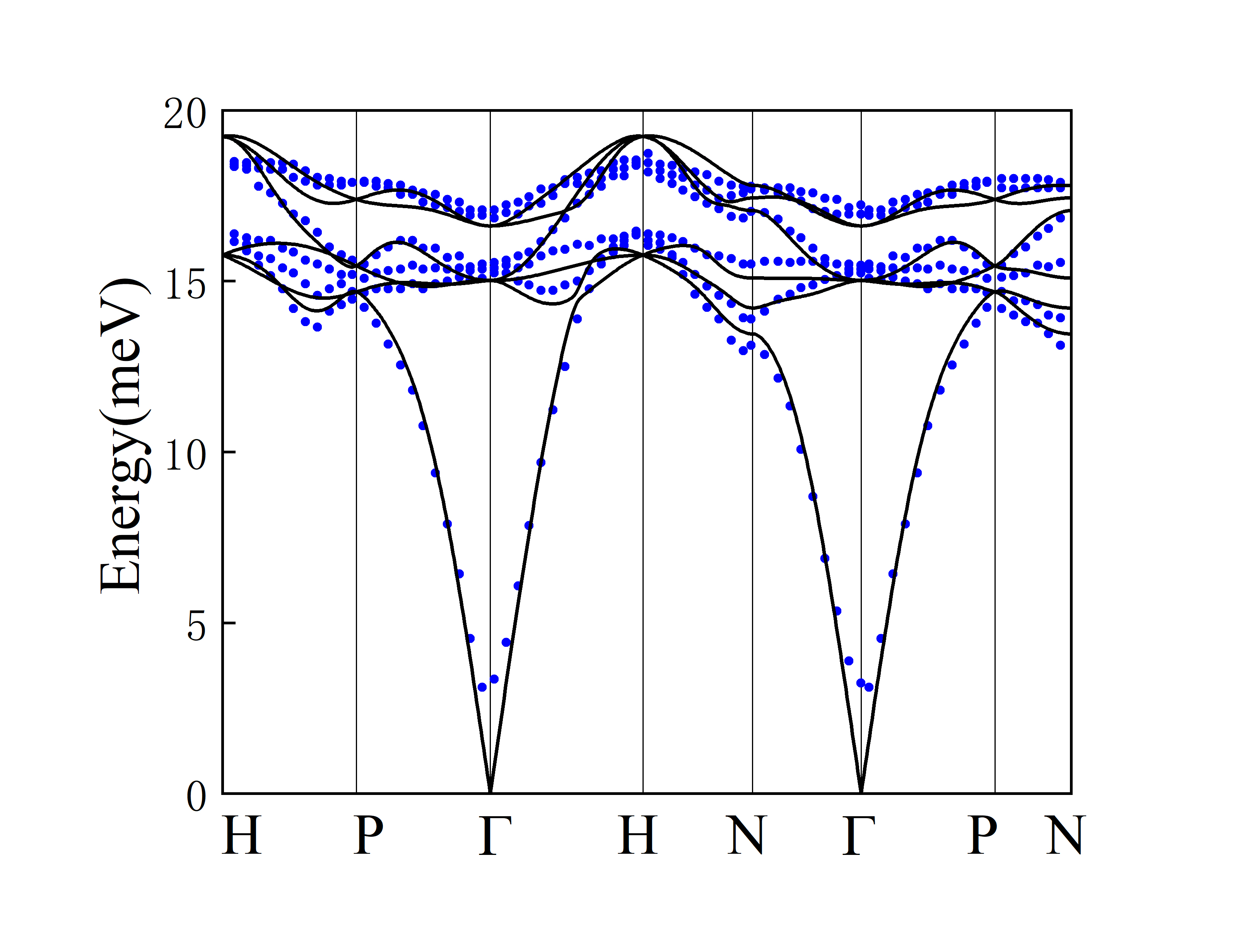
Figure 4: Calculated spin-wave dispersion curves along high-symmetry axis for Cu₃TeO₆. The INS spectra in Ref. Yao et al. (2018) are also shown as discrete points for comparison.

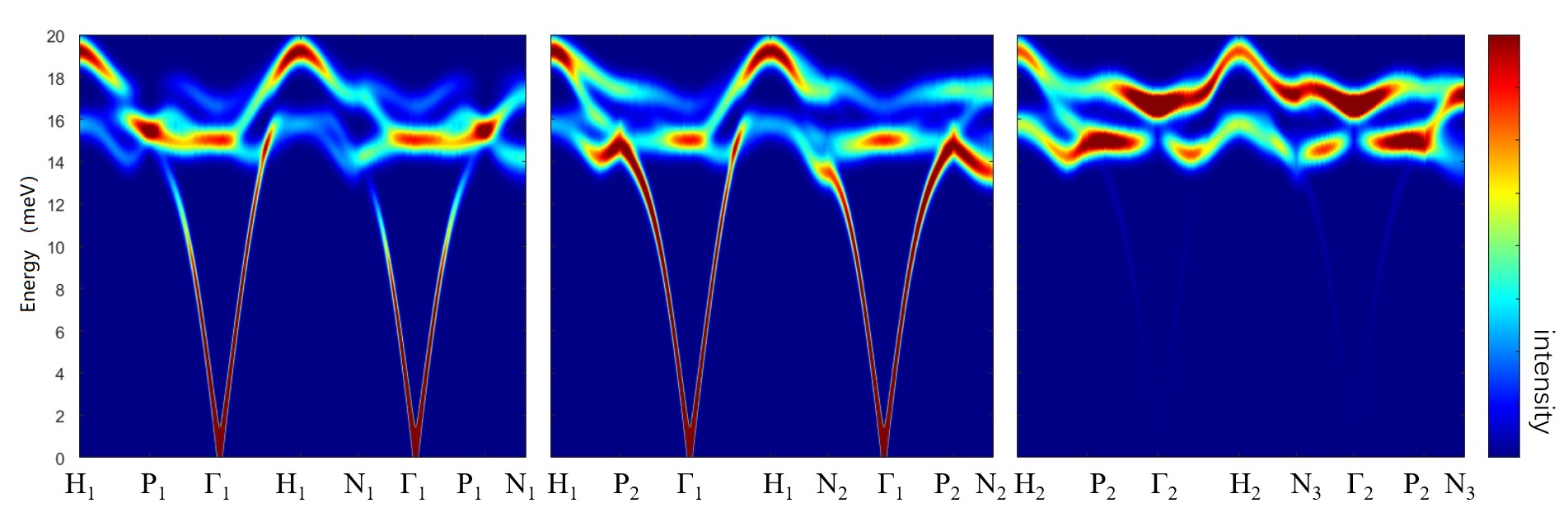
Figure 5: Calculated magnon spectra for Cu₃TeO₆  along three different momentum trajectories. The positions of high-symmetry points in reciprocal lattice units are $H_{1}$(2,1,2), $H_{2}$(1,0,2), $P_{1}$($\frac{3}{2}$,$\frac{3}{2}$,$\frac{3}{2}$), $P_{2}$($\frac{3}{2}$,$\frac{1}{2}$,$\frac{3}{2}$), $\Gamma_{1}$(1,1,2), $\Gamma_{2}$(2,0,2), $N_{1}$($\frac{3}{2}$,$\frac{3}{2}$,2), $N_{2}$($\frac{3}{2}$,1,$\frac{3}{2}$), and $N_{3}$($\frac{3}{2}$,0,$\frac{3}{2}$), respectively.

Based on the calculated electronic structures, we estimate the spin exchange parameters $J^{\prime}s$ (we refer to the exchange interaction of the $i$th NN as $J_{i}$) Wan et al. (2006). The FPLR approach allows us to calculate long-range exchange interactions accurately, and the results show that these exchange parameters decrease rapidly with increasing distance. We summarize the results up to 20th NN interaction $J_{20}$ in Table 1. The fitted spin exchange parameters in the previous experimental work are also shown for comparison Yao et al. (2018); Bao et al. (2018). As the FPLR approach automatically incorporates all the symmetry restrictions on exchange interactions, we can distinguish the inequivalent $J^{\prime}$s even though their exchange pathes own the same distance, such as $J_{4}$ and $J_{5}$ shown in the Table 1. The results show that for the Cu-Cu bond with the distance more than 7 Å, the exchange interactions can be neglected and there are only several sizable terms, including $J_{1}$, $J_{2}$, $J_{4}$, $J_{9}$, and $J_{10}$ . The strongest terms $J_{1}$ and $J_{9}$ both favor antiferromagnetic ordering, which is compatible with the magnetic ground state, thus there is no frustration between them. On the contrary the rest three sizable terms $J_{2}$, $J_{4}$, and $J_{10}$ are not compatible with the magnetic ground states. Note that they are much smaller than $J_{1}$ and $J_{9}$ , which results in the modest frustration in Cu₃TeO₆ system, consistent with the experimental result Bao et al. (2018). Based on the obtained spin exchange parameters $J^{\prime}s$ as shown in the last column in Table 1, we calculate the Curie-Weiss temperature $\theta_{CW}$ using the mean-field approximation theory Smart (1966) and the calculated $\theta_{CW}$ is $-$147 K, comparable with several experimental values as $-130$ K Herak et al. (2005), $-165$ K Yao et al. (2018) and $-175$ K Bao et al. (2018).

Using LSWT, we also calculate the magnetic excitation spectra and show the spin-wave dispersion $\omega_{m}(\mathbf{q})$ ($m=1,2,\ldots,12$) along high-symmetry axis by solid lines in Fig. 4. For comparison the INS spectra in the previous experimental work Yao et al. (2018) are also shown as blue discrete points in Fig. 4. The calculated spin-wave dispersion is in well agreement with the experimental measurements. As shown in Fig. 1, there are 12 Cu ions in each primitive cell, resulting in 12 bands in magnetic excitations. It should be noted that, due to $\mathcal{P}\mathcal{T}$ symmetry, all the magnon branches are doubly degenerate and one can only see six branches as shown in Fig. 4. The acoustic branches extend up to about 15 meV, while the optical ones are mainly located between 15 and 20 meV. These six doubly-degenerate branches form three Dirac points at $P$ at 14.7 meV, 15.4 meV and 17.4 meV, respectively, which is in good agreement with experimental results of two points around 15 meV and one in 17.8 meV Yao et al. (2018). Our numerical results show that there is a Dirac point at $\Gamma$ point of 16.6 meV while the experimental spin wave dispersions suggest the point near 17 meV Yao et al. (2018). In addition, we also reproduce a triply degenerate node in 15.0 meV at $\Gamma$ point, as observed by Bao et al. Bao et al. (2018) at the same energy of 15 meV. At $H$ point, we reproduce two triply degenerate points are located at 15.8 meV and 19.2 meV, while the experimental band crossings appear at about 16 meV and 18.5 meV Bao et al. (2018). Overall, these results are in good agreement with the theoretical and experimental works Li et al. (2017); Yao et al. (2018); Bao et al. (2018).

Besides the spin wave dispersion, we also calculate the magnetic neutron scattering intensity $I(\mathbf{Q,\omega})$ as a function of momentum $\mathbf{Q}=\mathbf{q}+\mathbf{G}$ ($\mathbf{G}$ is a reciprocal lattice vector and $\mathbf{q}$ is in the 1st BZ) and energy $\omega$ by using spin-spin correlation function, as shown in Fig. 5(a)$-$(c). Note that, the magnetic neutron scattering intensities may be significantly different for different $\mathbf{G}$ at any giving $\mathbf{q}$. For comparison with the experiment Yao et al. (2018), we display $I(\mathbf{Q,\omega})$ along three momentum trajectories shown in Figs. 5. The results capture most of the features in the previous experiment Yao et al. (2018); Bao et al. (2018). For example, the INS intensities in Figs. 5(a) and (b) are distributed in both acoustic and optical branches, while the INS intensity in Fig. 5(c) is mainly located at the optical branches between 15 and 20 meV. At $\Gamma_{1}$(1,1,2) point, the INS intensity is mainly located at acoustic branch and the triply degenerate point, while the intensity at $\Gamma_{2}$(2,0,2) point appears mainly at the Dirac point of 16.6 meV. Both at $H_{1}$(2,1,2) and $H_{2}$(1,0,2) point, the intensity is mainly located at the branch of the highest energy. As $\mathbf{Q}$ moves from $P_{2}$($\frac{3}{2}$,$\frac{1}{2}$,$\frac{3}{2}$) to $H_{1}$(2,1,2), the main intensity is located at the lowest energy branch, as well as in the path $P_{2}(\frac{3}{2},\frac{1}{2},\frac{3}{2})-N_{2}$($\frac{3}{2}$,1,$\frac{3}{2}$). These results are consistent with the experimental works Yao et al. (2018); Bao et al. (2018).

In Ref. Yao et al. (2018), through checking the magnon eigenvalue $\omega_{m}(\mathbf{q})$ at four high symmetry points, $\Gamma=(0,0,0),P=(\frac{1}{2},\frac{1}{2},\frac{1}{2}),H=(0,1,0),N=(\frac{1}{2},\frac{1}{2},0)$, Yao et al obtained an interesting relation expressed by the following eigenvalue-version of compatibility relation:

$$\sum_{m}(\omega_{\Gamma,m}^{2}+4\omega_{P,m}^{2}+\omega_{H,m}^{2})=\sum_{m}6\omega_{N,m}^{2},$$ (1)

which they called “sum rule” and proved that it holds at least up to the 9th NN Yao et al. (2018). Such kind of sum rule is surprised to us for conventional compatibility relation is usually only about the symmetry representations. Hence in the following we analytically investigate whether there exists a general sum rule on earth. We adopt the Heisenberg magnetic model as written by $\hat{H}=\frac{1}{2}\sum_{l,n,l^{\prime},n^{\prime}}J(\mathbf{R}_{l}+\boldsymbol{\tau}_{n},\mathbf{R}_{l}^{\prime}+\boldsymbol{\tau_{n^{\prime}}})\mathbf{S}_{ln}\cdot\mathbf{S}_{l^{\prime}n^{\prime}}$ where $l,l^{\prime}$ label the unit cell and $n,n^{\prime}$ label the Cu ions: $n,n^{\prime}=1,2,\ldots,6$ represent Cu with up spin while $n,n^{\prime}=7,8,\ldots,12$ represent Cu with down spin. The positions for these Cu ions in the primitive unit cell are key for the following analysis, we thus shown them in Tables 1 of the Appendix. Based on the antiferromagnetic ground state and using the LSWT, the magnon spectra are obtained by diagonalizing the following matrix and then extracting the non-negative eigenvalues for genuine magnon excitations Toth and Lake (2015) :

$$\mathcal{H}_{SW}(\mathbf{q})=\left[\begin{array}[]{cc}\mathcal{J}(\mathbf{q})&\mathcal{J}^{\prime}(\mathbf{q})\\ -\mathcal{J}^{\prime{\dagger}}(\mathbf{q})&-\mathcal{J}(-\mathbf{q})^{\top}\end{array}\right],$$ (2)

where $\mathcal{J}(\mathbf{q})$ and $\mathcal{J}^{\prime}(\mathbf{q})$ (both are 12$\times$12 matrices) are expressed by:

$$\mathcal{J}(\mathbf{q})_{n,n^{\prime}}=\zeta(n,n^{\prime})\sum_{l}J(\boldsymbol{\tau}_{n},\boldsymbol{\tau}_{n^{\prime}}+\mathbf{R}_{l})e^{i\mathbf{q}\cdot\mathbf{R}_{l}}+\delta_{n,n^{\prime}}[\sum_{l,n^{\prime\prime}}J(\boldsymbol{\tau}_{n},\boldsymbol{\tau}_{n^{\prime\prime}}+\mathbf{R}_{l})-\sum_{l,n^{\prime\prime\prime}}J(\boldsymbol{\tau}_{n},\boldsymbol{\tau}_{n^{\prime\prime\prime}}+\mathbf{R}_{l})],$$ (3)

$$\mathcal{J}^{\prime}(\mathbf{q})_{n,n^{\prime}}=\zeta^{\prime}(n,n^{\prime})\sum_{l}J(\boldsymbol{\tau}_{n},\boldsymbol{\tau}_{n^{\prime}}+\mathbf{R}_{l})e^{i\mathbf{q}\cdot\mathbf{R}_{l}},$$ (4)

where $\delta_{n,n^{\prime}}$ is the Kronecker delta function, $n^{\prime\prime}$ runs through the Cu ions with spins parallel to that of the $n$th Cu while $n^{\prime\prime\prime}$ runs through ions with spins antiparallel to that of the $n$th Cu. $\zeta(n,n^{\prime})$ ($\zeta^{\prime}(n,n^{\prime})$) is equal to 1 when the spins for the $n$th and $n^{\prime}$th Cu’s are parallel (antiparallel) otherwise equal to zero. Note that $\sum_{m}\omega_{m}(\mathbf{q})^{2}=tr(\mathcal{H}_{SW}^{2})$, thus Eq. (1) can be written in the following form:

$$tr(\mathcal{H}_{SW}(\Gamma)^{2}+\mathcal{H}_{SW}(H)^{2}+4\mathcal{H}_{SW}(P)^{2}-6\mathcal{H}_{SW}(N)^{2})=0.$$ (5)

Firstly we consider the 1st NN. For Cu ion labelled by $n=1$, there are four 1st NNs, as shown in the first 4 rows of the Table 2 of the Appendix. Cu ions in this compound occupy the 24$d$ Wyckoff positions, and there are in total 24 Cu-Cu 1st NN bonds as also listed in Table 2 of the Appendix. We use $(n,n^{\prime},R_{l})$ to denote the bond formed by the Cu ions labeled by $\tau_{n}$ and $\tau_{n^{\prime}}+R_{l}$. With these data, we can obtain all the matrix elements of $H_{SW}$ for any given $\mathbf{q}$. For each pair $(n,n^{\prime})$ of Cu ions, there is at most one nearest-neighbor exchange path connecting them as shown in Table 2. For the mentioned four high symmetry points, the nondiagonal matrix elements of $\mathcal{H}_{SW}$ are found to be one of the following values $\pm J_{1}$, or $\pm iJ_{1}$, or 0. While the diagonal matrix elements are equal to a constant for any $\mathbf{q}$. Therefore we prove that $tr(\mathcal{H}_{SW}(\Gamma)^{2})=tr(\mathcal{H}_{SW}(H)^{2})=tr(\mathcal{H}_{P}(\Gamma)^{2})=tr(\mathcal{H}_{SW}(N)^{2})$ and Eq. (5) is satisfied for the 1st NN. Similarly, we can prove that Eq. (5) holds from the $2$th NN to the $11$th NN. Further we can prove that Eq. (1) holds with the exchanges up to 11th NNs. However for the 12th NN, as shown in Table 3 of the Appendix, for each pair $(n,n^{\prime})$, there may exist 4 exchange pathes connecting them, so the corresponding matrix element of $\mathcal{H}_{SW}/J_{12}$ are the summation of four terms by Eqs. (3) and (4). This situation is different from that for the 1st NN, and one can easily prove that Eq. (5) is no longer right for 12th NNs. Therefore the “sum rule” (i.e. Eq. (1)) holds but only up to the 11th NNs.

It is worth mentioning that, though the Cu₃TeO₆ system has a global inversion center, most of the Cu-Cu bonds don’t own inversion symmetry. Within the distance of 7 Å, only the DMIs for 5th NN and 11th NN are required to be vanishing because their bonds have inversion center. Using the FPLR approach Wan et al. (2006), we calculate the DMIs. Since the strength of DMI is proportional to the corresponding $J$, we only calculate the $D_{1}$ and $D_{9}$ (we refer to the DMI of the $i$th NN as $D_{i}$). The $D_{1}$ for the Cu-Cu bond between (0, 0.25, 0.969) and ($-$0.031, 0.5, 0.75) in the coordinate system is estimated to be (0.05, 0.25, 0.34) meV. The direction of $D_{1}$ is nearly parallel to the normal direction of the triangle formed by the three atoms in the Cu-O-Cu bond, which is consistent with the physical expectation. While our calculation show that $D_{9}$ is very small ($\left|D_{9}\right|=0.06$ meV) and have little effect on the magnetic configuration. Our numerical ratio of $\left|D_{1}\right|/J_{1}$ is about 0.06, which is smaller than the pure theoretical model estimation (0.2) Li et al. (2017). The calculated DMIs result in a canting angle about 1.3^∘, which is in agreement with the experimental value $\sim$6^∘ Herak et al. (2005). The size of the nodal line is proportional to square of the ratio of DMI and $J$ Li et al. (2017), thus it is hard to identify the nodal lines from the Dirac points for the current experiments.

IV Conclusion

In conclusion, using first-principles calculation, we presented a comprehensive investigation of Cu₃TeO₆. The calculations show that Cu₃TeO₆ is an insulator with a band gap about 2.07 eV and the calculated magnetic moment of the Cu ions is 0.81 $\mu_{B}$. Using magnetic force theorem and a first-principles linear-response approach, we estimate the spin exchange parameters. The calculated exchange parameters are short-range and can be neglected for the distance more than 7 Å. The strongest terms $J_{1}$ and $J_{9}$ are compatible with the magnetic ground state, while the terms $J_{2}$, $J_{4}$, and $J_{10}$ are much smaller and not compatible with the magnetic ground states, which is consistent with the modest frustration in this compound. We calculated the magnon spectra using linear spin wave theory and the calculated spin wave is in good agreement with the experiment. We also prove analytically that the “sum rule” proposed in Ref. Yao et al. (2018) only holds up to the 11th nearest-neighbour interactions. The calculated DMIs lead to a very small canting angle about 1.3^∘ of non-collinear antiferromagnetic order. The weak DMIs are the possible reason why the previous experimental work did not observe the nodal lines.

V Acknowledgement

We wish to thank Prof. Yuan Li for discussion. The work was supported by National Key R&D Program of China (No. 2018YFA0305704 and 2017YFA0303203), the NSFC (No. 11525417, 11834006, 51721001 and 11790311), the Fundamental Research Funds for the Central Universities (No. 020414380085). DW was also supported by the program B for Outstanding PhD candidate of Nanjing University.

VI Appendix

In the Appendix, we list the coordinates of 12 Cu ions in Table 1.

$n$	$\boldsymbol{\tau}_{n}$
1	$(x,0,\frac{1}{4})$
2	$(\frac{1}{2}-x,0,\frac{3}{4})$
3	$(\frac{1}{4},x,0)$
4	$(\frac{3}{4},\frac{1}{2}-x,0)$
5	$(0,\frac{1}{4},x)$
6	$(0,\frac{3}{4},\frac{1}{2}-x)$
7	$(-x,0,-\frac{1}{4})$
8	$(\frac{1}{2}+x,0,\frac{1}{4})$
9	$(-\frac{1}{4},-x,0)$
10	$(\frac{1}{4},\frac{1}{2}+x,0)$
11	$(0,-\frac{1}{4},-x)$
12	$(0,\frac{1}{4},\frac{1}{2}+x)$

Table 1: The coordinates of the 12 Cu ions in the conventional unit cell basis vectors. $x=0.96907$.

According to Eqs. (2,3,4) of the main text, it is very easy to calculate the matrix $H_{SW}$ for any wave vector $q$ when knowing the full information of all the bonds. We thus give the detailed information of all the bonds connecting Cu ions for the 1st NN and 12th NN in Tables 2 and 3, respectively.

$n$	$n^{\prime}$	$\mathbf{R}_{l}$
1	9	$(1,1,0)$
1	10	$(\frac{1}{2},-\frac{3}{2},\frac{1}{2})$
1	11	$(1,0,1)$
1	12	$(1,0,-1)$
2	9	$(0,1,1)$
2	10	$(\frac{1}{2},-\frac{3}{2},\frac{1}{2})$
2	11	$(-\frac{1}{2},\frac{1}{2},\frac{3}{2})$
2	12	$(-\frac{1}{2},-\frac{1}{2},-\frac{1}{2})$
3	7	$(1,1,0)$
3	8	$(-1,1,0)$
3	11	$(0,1,1)$
3	12	$(\frac{1}{2},\frac{1}{2},-\frac{3}{2})$
4	7	$(\frac{3}{2},-\frac{1}{2},\frac{1}{2})$
4	8	$(-\frac{1}{2},-\frac{1}{2},-\frac{1}{2})$
4	11	$(1,0,1)$
4	12	$(\frac{1}{2},-\frac{1}{2},-\frac{3}{2})$
5	7	$(1,0,1)$
5	8	$(-\frac{3}{2},-\frac{1}{2},\frac{1}{2})$
5	9	$(0,1,1)$
5	10	$(0,-1,1)$
6	7	$(1,1,0)$
6	8	$(-\frac{3}{2},\frac{1}{2},-\frac{1}{2})$
6	9	$(\frac{1}{2},\frac{3}{2},-\frac{1}{2})$
6	10	$(-\frac{1}{2},-\frac{1}{2},-\frac{1}{2})$

Table 2: The 24 bonds for the first NN: each bond is characterized by the positions of the two endings: $\boldsymbol{\tau}_{n},\boldsymbol{\tau}_{n^{\prime}}+\mathbf{R}_{l}$.

$n$	$n^{\prime}$	$\mathbf{R}_{l}$
1	8	$(-\frac{1}{2},-\frac{1}{2},-\frac{1}{2})$
1	8	$(-\frac{1}{2},\frac{1}{2},\frac{1}{2})$
1	8	$(-\frac{1}{2},-\frac{1}{2},\frac{1}{2})$
1	8	$(-\frac{1}{2},\frac{1}{2},-\frac{1}{2})$
2	7	$(\frac{1}{2},\frac{1}{2},\frac{1}{2})$
2	7	$(\frac{1}{2},-\frac{1}{2},\frac{3}{2})$
2	7	$(\frac{1}{2},-\frac{1}{2},\frac{1}{2})$
2	7	$(\frac{1}{2},\frac{1}{2},\frac{3}{2})$
3	10	$(-\frac{1}{2},-\frac{1}{2},-\frac{1}{2})$
3	10	$(\frac{1}{2},-\frac{1}{2},\frac{1}{2})$
3	10	$(-\frac{1}{2},-\frac{1}{2},\frac{1}{2})$
3	10	$(\frac{1}{2},-\frac{1}{2},-\frac{1}{2})$
4	9	$(\frac{1}{2},\frac{1}{2},\frac{1}{2})$
4	9	$(\frac{3}{2},\frac{1}{2},-\frac{1}{2})$
4	9	$(\frac{1}{2},\frac{1}{2},-\frac{1}{2})$
4	9	$(\frac{3}{2},\frac{1}{2},\frac{1}{2})$
5	12	$(-\frac{1}{2},-\frac{1}{2},-\frac{1}{2})$
5	12	$(\frac{1}{2},\frac{1}{2},-\frac{1}{2})$
5	12	$(\frac{1}{2},-\frac{1}{2},-\frac{1}{2})$
5	12	$(-\frac{1}{2},\frac{1}{2},-\frac{1}{2})$
6	11	$(\frac{1}{2},\frac{1}{2},\frac{1}{2})$
6	11	$(-\frac{1}{2},\frac{3}{2},\frac{1}{2})$
6	11	$(-\frac{1}{2},\frac{1}{2},\frac{1}{2})$
6	11	$(\frac{1}{2},\frac{3}{2},\frac{1}{2})$

Table 3: The 24 bonds for the 12th NN: each bond is characterized by the positions of the two endings: $\boldsymbol{\tau}_{n},\boldsymbol{\tau}_{n^{\prime}}+\mathbf{R}_{l}$

References

- Hasan and Kane (2010) M. Z. Hasan and C. L. Kane, “Colloquium: topological insulators,” Rev. Mod. Phys. 82, 3045 (2010).
- Qi and Zhang (2011) X.-L. Qi and S.-C. Zhang, “Topological insulators and superconductors,” Rev. Mod. Phys. 83, 1057 (2011).
- Young et al. (2012) S. M. Young, S. Zaheer, J. C. Teo, C. L. Kane, E. J. Mele, and A. M. Rappe, “Dirac semimetal in three dimensions,” Phys. Rev. Lett. 108, 140405 (2012).
- Wang et al. (2012) Z. Wang, Y. Sun, X.-Q. Chen, C. Franchini, G. Xu, H. Weng, X. Dai, and Z. Fang, “Dirac semimetal and topological phase transitions in A3Bi (A= Na, K, Rb),” Phys. Rev. B 85, 195320 (2012).
- Wang et al. (2013) Z. Wang, H. Weng, Q. Wu, X. Dai, and Z. Fang, “Three-dimensional Dirac semimetal and quantum transport in Cd3As2,” Phys. Rev. B 88, 125427 (2013).
- Gibson et al. (2015) Q. D. Gibson, L. M. Schoop, L. Muechler, L. S. Xie, M. Hirschberger, N. P. Ong, R. Car, and R. J. Cava, “Three-dimensional Dirac semimetals: Design principles and predictions of new materials,” Phys. Rev. B 91, 205128 (2015).
- Du et al. (2015) Y. Du, B. Wan, D. Wang, L. Sheng, C.-G. Duan, and X. Wan, “Dirac and Weyl Semimetal in XYBi (X= Ba, Eu; Y= Cu, Ag and Au),” Sci. Rep. 5, 14423 (2015).
- Yang and Nagaosa (2014) B.-J. Yang and N. Nagaosa, “Classification of stable three-dimensional Dirac semimetals with nontrivial topology,” Nat. Commun. 5, 4898 (2014).
- Wan et al. (2011a) X. Wan, A. M. Turner, A. Vishwanath, and S. Y. Savrasov, “Topological semimetal and Fermi-arc surface states in the electronic structure of pyrochlore iridates,” Phys. Rev. B 83, 205101 (2011a).
- Huang et al. (2015) S.-M. Huang, S.-Y. Xu, I. Belopolski, C.-C. Lee, G. Chang, B. Wang, N. Alidoust, G. Bian, M. Neupane, C. Zhang, S. Jia, A. Bansil, H. Lin, and M. Z. Hasan, “A Weyl Fermion semimetal with surface Fermi arcs in the transition metal monopnictide TaAs class,” Nat. Commun. 6, 7373 (2015).
- Weng et al. (2015a) H. Weng, C. Fang, Z. Fang, B. A. Bernevig, and X. Dai, “Weyl semimetal phase in noncentrosymmetric transition-metal monophosphides,” Phys. Rev. X 5, 011029 (2015a).
- Burkov et al. (2011) A. A. Burkov, M. D. Hook, and L. Balents, “Topological nodal semimetals,” Phys. Rev. B 84, 235126 (2011).
- Weng et al. (2015b) H. Weng, Y. Liang, Q. Xu, R. Yu, Z. Fang, X. Dai, and Y. Kawazoe, “Topological node-line semimetal in three-dimensional graphene networks,” Phys. Rev. B 92, 045108 (2015b).
- Yu et al. (2015) R. Yu, H. Weng, Z. Fang, X. Dai, and X. Hu, “Topological node-line semimetal and Dirac semimetal state in antiperovskite Cu3PdN,” Phys. Rev. Lett. 115, 036807 (2015).
- Kim et al. (2015) Y. Kim, B. J. Wieder, C. L. Kane, and A. M. Rappe, “Dirac line nodes in inversion-symmetric crystals,” Phys. Rev. Lett. 115, 036806 (2015).
- Du et al. (2017) Y. Du, F. Tang, D. Wang, L. Sheng, E.-j. Kan, C.-G. Duan, S. Y. Savrasov, and X. Wan, “CaTe: a new topological node-line and Dirac semimetal,” npj Quant. Mater. 2, 3 (2017).
- Bansil et al. (2016) A. Bansil, H. Lin, and T. Das, “Colloquium: Topological band theory,” Rev. Mod. Phys. 88, 021004 (2016).
- Ando and Fu (2015) Y. Ando and L. Fu, “Topological crystalline insulators and topological superconductors: from concepts to materials,” Annu. Rev. Condens. Matter Phys. 6, 361–381 (2015).
- Wang et al. (2016) Z. Wang, A. Alexandradinata, R. J. Cava, and B. A. Bernevig, “Hourglass fermions,” Nature 532, 189 (2016).
- Slager et al. (2013) R.-J. Slager, A. Mesaros, V. Jurii, and J. Zaanen, “The space group classification of topological band-insulators,” Nature Physics 9, 98–102 (2013).
- Langbehn et al. (2017) J. Langbehn, Y. Peng, L. Trifunovic, F. von Oppen, and P. W. Brouwer, “Reflection-symmetric second-order topological insulators and superconductors,” Phys. Rev. Lett. 119, 246401 (2017).
- Song et al. (2017) Z. Song, Z. Fang, and C. Fang, “(d- 2)-Dimensional Edge States of Rotation Symmetry Protected Topological States,” Phys. Rev. Lett. 119, 246402 (2017).
- Benalcazar et al. (2017) W. A. Benalcazar, B. A. Bernevig, and T. L. Hughes, “Electric multipole moments, topological multipole moment pumping, and chiral hinge states in crystalline insulators,” Phys. Rev. B 96, 245115 (2017).
- Bzdek et al. (2016) T. Bzdek, Q. Wu, A. Regg, M. Sigrist, and A. A. Soluyanov, “Nodal-chain metals,” Nature 538, 75–78 (2016).
- Po et al. (2017) H. C. Po, A. Vishwanath, and H. Watanabe, “Symmetry-based indicators of band topology in the 230 space groups,” Nat. Commun. 8, 50 (2017).
- Bradlyn et al. (2017) B. Bradlyn, L. Elcoro, J. Cano, M. G. Vergniory, Z. Wang, C. Felser, M. I. Aroyo, and B. A. Bernevig, “Topological quantum chemistry,” Nature 547, 298 (2017).
- Kruthoff et al. (2017) J. Kruthoff, J. de Boer, J. van Wezel, C. L. Kane, and R.-J. Slager, “Topological classification of crystalline insulators through band structure combinatorics,” Phys. Rev. X 7, 041069 (2017).
- Watanabe et al. (2018) H. Watanabe, H. C. Po, and A. Vishwanath, “Structure and topology of band structures in the 1651 magnetic space groups,” Sci. Adv. 4, eaat8685 (2018).
- Tang et al. (2018a) F. Tang, H. C. Po, A. Vishwanath, and X. Wan, “Towards ideal topological materials: Comprehensive database searches using symmetry indicators,” ArXiv e-prints (2018a), arXiv:1807.09744 .
- Tang et al. (2018b) F. Tang, H. C. Po, A. Vishwanath, and X. Wan, “Efficient Topological Materials Discovery Using Symmetry Indicators,” ArXiv e-prints (2018b), arXiv:1805.07314 .
- Vergniory et al. (2018) M. G. Vergniory, L. Elcoro, C. Felser, B. A. Bernevig, and Z. Wang, “The (High Quality) Topological Materials In The World,” ArXiv e-prints (2018), arXiv:1807.10271 .
- Zhang et al. (2018) T. Zhang, Y. Jiang, Z. Song, H. Huang, Y. He, Z. Fang, H. Weng, and C. Fang, “Catalogue of Topological Electronic Materials,” ArXiv e-prints (2018), arXiv:1807.08756 .
- Lu et al. (2014) L. Lu, J. D. Joannopoulos, and M. Soljačić, “Topological photonics,” Nat. Photonics 8, 821 (2014).
- Zilberberg et al. (2018) O. Zilberberg, S. Huang, J. Guglielmon, M. Wang, K. P. Chen, Y. E. Kraus, and M. C. Rechtsman, “Photonic topological boundary pumping as a probe of 4D quantum Hall physics,” Nature 553, 59 (2018).
- Zhou et al. (2018) H. Zhou, C. Peng, Y. Yoon, C. W. Hsu, K. A. Nelson, L. Fu, J. D. Joannopoulos, M. Soljačić, and B. Zhen, “Observation of bulk Fermi arc and polarization half charge from paired exceptional points,” Science 359, 1009–1012 (2018).
- Yang et al. (2018) B. Yang, Q. Guo, B. Tremain, R. Liu, L. E. Barr, Q. Yan, W. Gao, H. Liu, Y. Xiang, J. Chen, C. Fang, A. Hibbins, L. Lu, and S. Zhang, “Ideal Weyl points and helicoid surface states in artificial photonic crystal structures,” Science 359, 1013–1016 (2018).
- Stenull et al. (2016) O. Stenull, C. L. Kane, and T. C. Lubensky, “Topological phonons and weyl lines in three dimensions,” Phys. Rev. Lett. 117, 068001 (2016).
- Serra-Garcia et al. (2018) M. Serra-Garcia, V. Peri, R. Süsstrunk, O. R. Bilal, T. Larsen, L. G. Villanueva, and S. D. Huber, “Observation of a phononic quadrupole topological insulator,” Nature 555, 342 (2018).
- Mook et al. (2014) A. Mook, J. Henk, and I. Mertig, “Edge states in topological magnon insulators,” Phys. Rev. B 90, 024412 (2014).
- Zhang et al. (2013) L. Zhang, J. Ren, J.-S. Wang, and B. Li, “Topological magnon insulator in insulating ferromagnet,” Phys. Rev. B 87, 144101 (2013).
- Fransson et al. (2016) J. Fransson, A. M. Black-Schaffer, and A. V. Balatsky, “Magnon dirac materials,” Phys. Rev. B 94, 075401 (2016).
- Owerre (2017) S. A. Owerre, “Magnonic analogs of topological Dirac semimetals,” J. Phys. Commun. 1, 025007 (2017).
- Pershoguba et al. (2018) S. S. Pershoguba, S. Banerjee, J. C. Lashley, J. Park, H. Ågren, G. Aeppli, and A. V. Balatsky, “Dirac magnons in honeycomb ferromagnets,” Phys. Rev. X 8, 011010 (2018).
- Li et al. (2016) F.-Y. Li, Y.-D. Li, Y. B. Kim, L. Balents, Y. Yu, and G. Chen, “Weyl magnons in breathing pyrochlore antiferromagnets,” Nat. Commun. 7, 12691 (2016).
- Mook et al. (2016) A. Mook, J. Henk, and I. Mertig, “Tunable magnon Weyl points in ferromagnetic pyrochlores,” Phys. Rev. Lett. 117, 157204 (2016).
- Su et al. (2017) Y. Su, X. S. Wang, and X. R. Wang, “Magnonic Weyl semimetal and chiral anomaly in pyrochlore ferromagnets,” Phys. Rev. B 95, 224403 (2017).
- Li et al. (2017) K. Li, C. Li, J. Hu, Y. Li, and C. Fang, “Dirac and nodal line magnons in three-dimensional antiferromagnets,” Phys. Rev. Lett. 119, 247202 (2017).
- Hostachy and Coing-Boyat (1968) A. Hostachy and J. Coing-Boyat, “Structure cristalline de Cu3TeO6,” CR Acad. Sci. Paris 267, 1435 (1968).
- Falck et al. (1978) L. Falck, O. Lindqvist, and J. Moret, “Tricopper (ii) tellurate (vi),” Acta Crystallographica Section B: Structural Crystallography and Crystal Chemistry 34, 896–897 (1978).
- Herak et al. (2005) M. Herak, H. Berger, M. Prester, M. Miljak, I. Živković, O. Milat, D. Drobac, S. Popović, and O. Zaharko, “Novel spin lattice in Cu3TeO6: an antiferromagnetic order and domain dynamics,” J. Phys. Condens. Matter 17, 7667 (2005).
- Månsson et al. (2012) M. Månsson, K. Prša, J. Sugiyama, D. Andreica, H. Luetkens, and H. Berger, “Magnetic order and transitions in the spin-web compound Cu3TeO6,” Physics Procedia 30, 142–145 (2012).
- Yao et al. (2018) W. Yao, C. Li, L. Wang, S. Xue, Y. Dan, K. Iida, K. Kamazawa, K. Li, C. Fang, and Y. Li, “Topological spin excitations in a three-dimensional antiferromagnet,” Nat. Phys. 14, 1011 (2018).
- Bao et al. (2018) S. Bao, J. Wang, W. Wang, Z. Cai, S. Li, Z. Ma, D. Wang, K. Ran, Z.-Y. Dong, D. L. Abernathy, S.-L. Yu, X. Wan, J.-X. Li, and J. Wen, “Discovery of coexisting Dirac and triply degenerate magnons in a three-dimensional antiferromagnet,” Nat. Commun. 9, 2591 (2018).
- Bradlyn et al. (2016) B. Bradlyn, J. Cano, Z. Wang, M. G. Vergniory, C. Felser, R. J. Cava, and B. A. Bernevig, “Beyond Dirac and Weyl fermions: Unconventional quasiparticles in conventional crystals,” Science 353, aaf5037 (2016).
- Lv et al. (2017) B. Q. Lv, Z.-L. Feng, Q.-N. Xu, X. Gao, J.-Z. Ma, L.-Y. Kong, P. Richard, Y.-B. Huang, V. N. Strocov, C. Fang, H.-M. Weng, Y.-G. Shi, T. Qian, and H. Ding, “Observation of three-component fermions in the topological semimetal molybdenum phosphide,” Nature 546, 627 (2017).
- Dzyaloshinsky (1958) I. Dzyaloshinsky, “A thermodynamic theory of weak ferromagnetism of antiferromagnetics,” J. Phys. Chem. Solids 4, 241–255 (1958).
- Moriya (1960) T. Moriya, “Anisotropic superexchange interaction and weak ferromagnetism,” Phys. Rev. 120, 91 (1960).
- Wan et al. (2006) X. Wan, Q. Yin, and S. Y. Savrasov, “Calculation of magnetic exchange interactions in mott-hubbard systems,” Phys. Rev. Lett. 97, 266403 (2006).
- Blaha et al. (2001) P. Blaha, K. Schwarz, G. Madsen, D. Kvasnicka, and J. Luitz, WIEN2k, An augmented plane wave+ Local Orbitals Program for calculating Crystal Properties (Karlheinz Schwarz, TU Wien, Austria, 2001).
- Koelling and Harmon (1977) D. D. Koelling and B. N. Harmon, “A technique for relativistic spin-polarised calculations,” J. Phys. C 10, 3107 (1977).
- Anisimov et al. (1997) V. I. Anisimov, F. Aryasetiawan, and A. I. Lichtenstein, “First-principles calculations of the electronic structure and spectra of strongly correlated systems: the LDA+U method,” J. Phys. Condens. Matter 9, 767 (1997).
- Anisimov et al. (2002) V. I. Anisimov, M. A. Korotin, I. A. Nekrasov, Z. V. Pchelkina, and S. Sorella, “First principles electronic model for high-temperature superconductivity,” Phys. Rev. B 66, 100502 (2002).
- Wan et al. (2009) X. Wan, T. A. Maier, and S. Y. Savrasov, “Calculated magnetic exchange interactions in high-temperature superconductors,” Phys. Rev. B 79, 155114 (2009).
- Liechtenstein et al. (1987) A. I. Liechtenstein, M. I. Katsnelson, V. P. Antropov, and V. A. Gubanov, “Local spin density functional approach to the theory of exchange interactions in ferromagnetic metals and alloys,” J. Magn. Magn. Mater. 67, 65–74 (1987).
- Frota-Pessôa et al. (2000) S. Frota-Pessôa, R. B. Muniz, and J. Kudrnovskỳ, “Exchange coupling in transition-metal ferromagnets,” Phys. Rev. B 62, 5293 (2000).
- Pajda et al. (2001) M. Pajda, J. Kudrnovskỳ, I. Turek, V. Drchal, and P. Bruno, “Ab initio calculations of exchange interactions, spin-wave stiffness constants, and Curie temperatures of Fe, Co, and Ni,” Phys. Rev. B 64, 174402 (2001).
- Fischer et al. (2009) G. Fischer, M. Däne, A. Ernst, P. Bruno, M. Lüders, Z. Szotek, W. Temmerman, and W. Hergert, “Exchange coupling in transition metal monoxides: Electronic structure calculations,” Phys. Rev. B 80, 014408 (2009).
- Galanakis and Şaşıoğlu (2012) I. Galanakis and E. Şaşıoğlu, “Ab-initio calculation of effective exchange interactions, spin waves, and Curie temperature in L21-and L12-type local moment ferromagnets,” J. Mater. Sci. 47, 7678–7685 (2012).
- Mazurenko and Anisimov (2005) V. V. Mazurenko and V. I. Anisimov, “Weak ferromagnetism in antiferromagnets: - Fe2O3 and La2CuO4,” Phys. Rev. B 71, 184434 (2005).
- Katsnelson et al. (2010) M. I. Katsnelson, Y. O. Kvashnin, V. V. Mazurenko, and A. I. Lichtenstein, “Correlated band theory of spin and orbital contributions to Dzyaloshinskii-Moriya interactions,” Phys. Rev. B 82, 100403 (2010).
- Wan et al. (2011b) X. Wan, J. Dong, and S. Y. Savrasov, “Mechanism of magnetic exchange interactions in europium monochalcogenides,” Phys. Rev. B 83, 205201 (2011b).
- Kotliar et al. (2006) G. Kotliar, S. Y. Savrasov, K. Haule, V. S. Oudovenko, O. Parcollet, and C. A. Marianetti, “Electronic structure calculations with dynamical mean-field theory,” Rev. Mod. Phys. 78, 865 (2006).
- Smart (1966) J. S. Smart, Effective field theories of magnetism, 2 (Saunders, 1966).
- Toth and Lake (2015) S. Toth and B. Lake, “Linear spin wave theory for single-Q incommensurate magnetic structures,” J. Phys. Condens. Matter 27, 166002 (2015).