Unraveling the structure of treelike networks from first-passage times of lazy random walkers

Abstract

We study the problem of random search in finite networks with a tree topology, where it is expected that the distribution of the first-passage time $F(t)$ decays exponentially. We show that the slope $\alpha$ of the exponential tail is independent of the initial conditions of entering the tree in general, and scales exponentially or as a power law with the extent of the tree $L$, depending on the tendency $p$ to jump toward the target node. It is unfeasible to uniquely determine $L$ and $p$ from measuring $\alpha$ or the mean first-passage time (MFPT) of an ordinary diffusion along the tree. To unravel the structure, we consider lazy random walkers that take steps with probability $m$ when jumping on the nodes and return with probability $q$ from the leaves. By deriving an exact analytical expression for the MFPT of the intermittent random walk, we verify that the structural information of the tree can be uniquely extracted by measuring the MFPT for two randomly chosen types of tracer particles with distinct experimental parameters $m$ and $q$. We also address the applicability of our approach in the presence of disorder in the structure of the tree or statistical uncertainty in the experimental parameters.

I Introduction

Diffusion and transport in complex environments are strongly influenced by the geometrical and topological properties of the underlying structures ben-Avraham00 . For example, the topology of the tree structure of human lung affects the absorption efficiency of diffusing oxygen Felici04 , the obstacle size and density determines the mean free path of light in turbid media Sadjadi , the topology of Cayley trees influences the average displacement of quantum or classical random walkers Agliara08 ; Agliara14 , or the arrangement of magnetic bubbles in flashing potentials controls the anomalous behavior of the mean square displacement of paramagnetic colloidal particles Tierno16 .

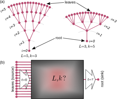
Figure 1: (a) Examples of finite regular trees with the same number of leaves but different structure. (b) Schematic illustration of the measurement design. The tracer particle enters a tree, with unknown structural characteristics $L$ and $k$ (more generally $p$), from a leaf. It performs a random walk and eventually reaches the root after a first-passage time $\tau$. The mean first-passage time $\langle\tau\rangle$ is obtained by repeating the measurement for an ensemble of noninteracting tracer particles.

Conversely, reconstructing the structure by means of the information obtained from the transport properties of tracer particles also constitutes an interesting subject. The idea of extracting the structural information of labyrinthine environments (or indirect evaluation of other quantities of interest in general) from the diffusional properties has attracted attention for a few decades Kac66 ; Mitra92 ; Mair99 ; Krishna09 ; Chen12 ; Cooper16 ; Agliari07 ; Durian91 ; Maret97 : (i) It was suggested Kac66 that the geometry of the boundaries of a drum can be determined from the eigenvalues of the diffusion equation in a cage surrounded by absorbing walls; (ii) in porous structures, the porosity Mitra92 , surface-to-volume ratio of the voids Mair99 , degree of confinement and absorption strength Krishna09 , and permeability Chen12 were shown to be calculable from the diffusion propagator (more simply from the asymptotic diffusion coefficient in special cases); (iii) the temporal changes in the structure of foams and turbid media can be probed by the diffusive propagation of light Durian91 ; Maret97 ; (iv) the geometrical properties of complex networks such as the number of triangles, loops, and subgraphs can be estimated from the first return time of random walks Cooper16 ; and (v) as the last example, the time required for autocatalytic reactions on inhomogeneous substrates can be obtained from the mean time taken for the reactants to reach a reaction center or to encounter each other Agliari07 .

In this paper, we verify that the mean first-passage time (MFPT) of tracer particles to reach a target, as a conceptually simple and easily accessible transport quantity, can be employed to extract useful structural information. While we consider a treelike network in the present study, the idea can be extended to other complex networks and structures Sood07 . Branching morphologies constitute an important subset of complex structures, ranging from real systems (e.g. dendrimer macromolecules Helfand83 ; Wu12 ; Heijs04 ; Katsoulis02 ; Argyrakis00 , neuronal dendrites Spruston08 ; Hering01 ; Jose18 , and rivers Fleury01 ) to virtual ones such as treelike graphs Szabo02 ; Bollobas04 . To investigate diffusion on branched structures, they have been often modeled as regular treelike networks with, e.g., a given degree of the node $k$ representing the number of links connected to each node [see Fig. 1(a)]. Well-studied examples include finite Cayley trees Helfand83 ; Wu12 ; Heijs04 ; Katsoulis02 ; Argyrakis00 ; Redner01 and infinite Bethe lattices Hughes82 ; Monthus96 ; Cassi89 . A weight can be also assigned to each link Yook01 ; Almaas05 , as the real-world networks exhibit heterogeneity in the capacity of their links Barrat04 ; Krause03 . The advantage of regular trees is that the stochastic transport of particles along such structures can be mapped onto effective one-dimensional random walk models. By mapping Bethe lattices and Cayley trees onto 1D random walks, some basic quantities such as the mean square displacement, the probability of returning to the origin, and the first-passage times were calculated Helfand83 ; Wu12 ; Heijs04 ; Katsoulis02 ; Argyrakis00 ; Hughes82 ; Monthus96 ; Cassi89 . For example, the MFPT to reach a target node in finite trees was shown to depend on the extent $L$ of the tree as well as the degree $k$ of the node (more generally on the probability $p$ to hop toward the target) Wu12 ; Heijs04 ; Khantha83 ; Skarpalezos13 . Thus, the structural parameters $L$ and $k$ [shown in Fig. 1(a)] cannot be uniquely determined from the measurement of the MFPT of an ordinary random walk on the tree. The question arises of whether the prediction of the structural properties of trees from the MFPTs of other types of random walks is feasible. It is also not clear how far the possible predictions are robust in the presence of disorder in the extent of the tree, the degree of the nodes, or the capacity of the links.

To be able to unravel the structure, we increase the complexity of the dynamics of the tracer particles by introducing lazy random walkers that intermittently jump along the tree. We derive an exact analytical expression for the MFPT in terms of the waiting probabilities at nodes and dead ends (leaves), which enables us to uniquely determine the structure by measuring the MFPTs [see the schematic sketch in Fig. 1(b)]. To identify the validity range of the theoretical results, we compare the analytical predictions to the simulation results in the presence of disorder in the structure of the tree or statistical uncertainty in the experimental parameters. Our results are also applicable to ordinary random walks along specific structures which induce temporal absorption along the path or at the dead ends. This is particularly relevant to transport in neuronal dendrites in the presence of biochemical cages along the dendritic tubes Spruston08 ; Hering01 ; Jose18 .

This paper is organized as follows. We first review biased random walks on bounded 1D domains and ordinary random walks on regularly branched trees in Sec. II, and present an expression for the MFPT to travel from the leaves to the root of a finite tree. Next we introduce lazy random walkers in Sec. III and demonstrate how the structure of the tree can be uniquely determined from the MFPTs of such tracer particles. In Sec. IV, we show how the deviation of the MFPT from that of a regular tree enhances as the structural disorder or the experimental uncertainty grows. Sec. V concludes the paper.

II First-passage times of biased random walks on finite 1D domains

Stochastic motion of biased Garcia-Pelayo07 ; Pottier96 ; Weiss02 ; Benichou99 ; Mehra02 or persistent Garcia-Pelayo07 ; Pottier96 ; Weiss02 ; Shaebani14 ; Masoliver89 walkers in one dimension has been thoroughly investigated in the literature. Several aspects of 1D random walks, such as the influence of waiting Hafner16 or absorption Benichou99 along the path or at the boundaries Kantor07 on transport properties, has been studied. These studies also help understand the transport in other systems. For example, mapping of Bethe lattices and Cayley trees onto 1D random walks facilitates the calculation of the transport quantities of interest such as the first-passage times. While the MFPT to visit any specific target node on the Bethe lattice (i.e. an unlimited Cayley tree) is infinite, the MFPT in bounded domains such as Cayley trees is finite Wu12 ; Heijs04 ; Khantha83 ; Skarpalezos13 . For instance, it was shown that the MFPT of traveling from the leaves to the root of a finite regular tree obeys the following relation Khantha83 ; Skarpalezos13

$$\langle\tau\rangle=\displaystyle\frac{L}{2p-1}+\displaystyle\frac{1-p}{(2p-1)^{2}}\Big{[}\big{(}\frac{1-p}{p}\big{)}^{L}{-}1\Big{]},$$ (1)

where $L$ denotes the extent of the tree and $p$ represents the tendency to hop toward the root at each node (corresponding to an effective bias toward the target in a 1D system). Here, the parameter $p$ equals to $p{=}\frac{1}{k}$ in trees with uniform links, where $k$ is the coordination number (i.e. the degree of the nodes) as shown in Fig. 1(a). More generaly, $p$ can represent the effective tendency to move toward the target including all the effects of branching at nodes, relative weights of the links, tendency to follow the shortest path toward the target, etc. The relevant systems are, e.g., weighted treelike networks Almaas05 , neuronal dendrites where the branches tend to taper toward the dead ends Jose18 , and stochastic packet transport in the Internet preferably along the shortest path Huisinga01 ; Kachhvah12 (though the latter structure contains loops). In deriving Eq. (1), it was assumed that the reflection probability at the dead ends (leaves) equals the hopping probability toward the root at the bulk nodes Khantha83 ; Skarpalezos13 .

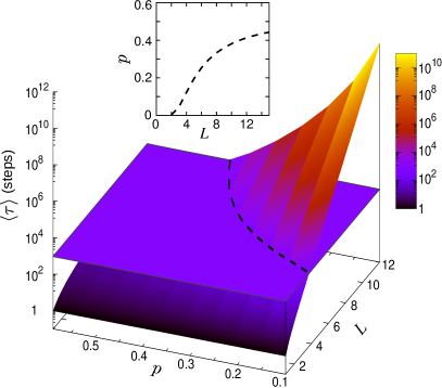
Figure 2: Mean first-passage time $\langle\tau\rangle$ of traveling from the leaves to the root, obtained via Eq. (1), versus the extent of the tree $L$ and the effective tendency $p$ to jump toward the target. The flat plane represents a constant MFPT, $\langle\tau\rangle{\simeq}1000\,\text{steps}$, as an example of the measured MFPT in experiments. The dashed contour line marks the intersection of the two surfaces, i.e. the path along which the MFPT equals the measured value. Inset: The contour line in the $(L,p)$ phase space.

According to Eq. (1), the MFPT depends on both $L$ and $p$ parameters. Therefore, having access to the MFPT via the experiment illustrated in Fig. 1(b) does not provide sufficient information to uniquely determine the structure, i.e. the tree extent $L$ and the node degree $k$ (or the effective upward tendency $p$). As shown in Fig. 2, for a given measured value of the MFPT, one obtains a monotonic iso-MFPT contour line in the $(L,p)$ phase space as the set of possible solutions.

III First-passage times of intermittent random walks

We propose that the structural properties of an unknown tree can be deduced from the mean first-passage times of specific tracer particles with a tunable tendency to move along the tree. We consider random walks with waiting probabilities at nodes and leaves. When such lazy random walkers enter a tree from the leaves, explore the unknown structure, and exit from the root, the MFPT can be obtained in terms of the waiting probabilities. We show that having access to the MFPT for only two different random choices of the waiting probabilities enables us to uniquely determine the structure of the regular tree via the analytical framework developed in this section.

Let us consider the stochastic motion of an individual random walker on the nodes of a regular tree with the extent $L$. We can identify each node by its generation (i.e. its distance from the root) in regular trees. The generation of the nodes ranges from $0$ at the root to $L$ at the leaves. The number of nodes belonging to the same generation $i$ equals $k^{i{-}1}$ (for $i{>}0$), with $k$ being the coordination number of the nodes. Each tracer particle initially enters the tree from one of the leaves. When being on a bulk node, it either jumps to one of the neighboring nodes with probability $m$ or waits at its current node with probability $1{-}m$ at each time step. The dynamics is however different at the boundaries. At the leaves, the particle either returns to the interior of the tree with probability $q$ or waits with probability $1{-}q$. The other boundary, i.e. the root node with generation $i{=}0$, is treated as a trap. When the particle eventually reaches the root after a first-passage time $\tau$, it is not allowed to return to the tree (which corresponds to $m{=}0$ for the specific generation $i{=}0$).

In trees with uniform links and in the absence of other sources which induce preferency toward the target, $k$ determines the probability $\frac{m}{k}$ to jump to one of the neighboring nodes, thus, the relative tendency to move toward the target equals $p{=}\frac{1}{k}$. More generally, there can exist an additional net probability $m^{\prime}$ to choose the root direction ($0{\leq}m^{\prime}{\leq}m$), induced by other possible effects (such as the hierarchical reduction of branch diameter toward the leaves or tendency to travel along the shortest path). In such a case, the total probability to jump from a bulk node toward the root or each of the leaves is $\frac{m{-}m^{\prime}}{k}{+}m^{\prime}$ or $\frac{m{-}m^{\prime}}{k}$, respectively. Therefore, the relative tendency to move toward the root effectively equals $p{=}\frac{m{-}m^{\prime}}{m}\frac{1}{k}{+}\frac{m^{\prime}}{m}$ and the tendency to hop to any of the nodes toward the leaves is $\frac{m{-}m^{\prime}}{m}\frac{1}{k}$.

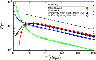
Figure 3: First-passage time distribution for $L{=}6$ and $p=m=q=0.5$ and for different initial conditions of entering the tree. The solid lines are the analytical prediction of Eq. (3) and the symbols denote the simulation results. The exponential dashed line is given by Eq. (4).

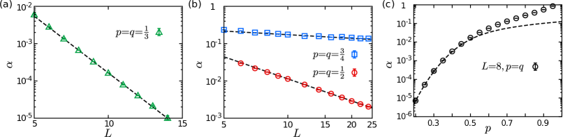
Figure 4: The slope $\alpha$ of the exponential tail versus the extent of the tree for (a) $p{<}\frac{1}{2}$ (log-lin scales) and (b) $p{\geq}\frac{1}{2}$ (log-log scales) at $m{=}1$. The dashed lines represent exponential or power-law fits. (c) $\alpha$ versus $p$ at $L{=}8$ and $m{=}1$. The dashed line represents $\alpha{=}1/\langle\tau\rangle$ for the MFPTs obtained for different values of $p$ at $L{=}8$, $m{=}1$, and $q{=}p$.

In the following, we solve the problem of the first-passage time from leaves to root for the set of parameters $\{L,p,m,q\}$. However, one can straightforwardly follow the proposed approach to calculate the MFPT between two arbitrary generations of the tree. By introducing the probability distribution $P\!\!_{{}_{i}}(t)$ of being on a node with generation $i$ at time step $t$, we practically map the problem onto an effective biased random walk on a 1D domain in the presence of temporal absorption along the path and at one of the boundaries. Using the initial condition $P\!\!_{{}_{i}}(0){=}\delta_{i,L}$, we construct a set of master equations for the dynamical evolution of $P\!\!_{{}_{i}}(t)$. The probability evolves at the root ($i{=}0$) and leaves ($i{=}L$) as $P\!\!_{{}_{0}}(t){=}P\!\!_{{}_{0}}(t{-}1){+}m\,p\,P\!\!_{{}_{1}}(t{-}1)$ and $P\!\!_{{}_{L}}(t){=}m\,(1{-}p)\,P\!\!_{{}_{L{-}1}}(t{-}1){+}(1{-}q)\,P\!\!_{{}_{L}}(t{-}1){+}\delta_{0,t}$. At a bulk node with generation $i$, the evolution of $P\!\!_{{}_{i}}(t)$ follows $P\!\!_{{}_{i}}(t){=}m\,(1{-}p)\,P\!\!_{{}_{i{-}1}}(t{-}1){+}(1{-}m)\,P\!\!_{{}_{i}}(t{-}1){+}m\,p\,P\!\!_{{}_{i{+}1}}(t{-}1)$. By defining the $z$ transform $P\!\!_{{}_{i}}(z){=}\sum\limits_{t{=}0}^{\infty}P\!\!_{{}_{i}}(t)\,z^{t}$, we obtain the following set of coupled equations

$$\left\{\begin{array}[]{ll}P\!\!_{{}_{0}}(z)&\!\!\!=z\,P\!\!_{{}_{0}}\!(z){+}m\,p\,z\,P\!\!_{{}_{1}}\!(z),\vspace{1mm}\\ P\!\!_{{}_{1}}(z)&\!\!\!=(1{-}m)z\,P\!\!_{{}_{1}}\!(z){+}m\,p\,z\,P\!\!_{{}_{2}}\!(z),\\ \;\;\;\;\Shortstack{...}&\\ P\!\!_{{}_{i}}(z)&\!\!\!=m(1{-}p)z\,P\!\!_{{}_{i{-}1}}\!(z){+}(1{-}m)z\,P\!\!_{{}_{i}}(z)\\ &\hskip 74.5462pt{+}m\,p\,z\,P\!\!_{{}_{i{+}1}}\!(z),\\ \;\;\;\;\Shortstack{...}&\\ P\!\!_{{}_{L{-}1}}\!(z)&\!\!\!=m(1{-}p)z\,P\!\!_{{}_{L{-}2}}\!(z){+}(1{-}m)z\,P\!\!_{{}_{L{-}1}}\!(z){+}q\,z\,P\!\!_{{}_{L}}\!(z),\vspace{1mm}\\ P\!\!_{{}_{L}}\!(z)&\!\!\!=m(1{-}p)z\,P\!\!_{{}_{L{-}1}}\!(z){+}(1{-}q)z\,P\!\!_{{}_{L}}\!(z){+}1.\end{array}\right.$$ (2)

After some algebra we obtain $P\!\!_{{}_{i}}(z)$ in the general form. Then, the $z$ transform of the FPT distribution to reach the root can be evaluated as $F(z){=}m\,p\,z\,P\!\!_{{}_{1}}(z)$ Redner01 . We derive an exact expression for the $z$ transform of the FPT distribution Jose18

$$F(z){=}\displaystyle\frac{2^{L+1}\,q\,A(z,m,p)}{\big{(}H_{+}^{L}{-}H_{-}^{L}\big{)}B(z,q,m,p){+}\big{(}H_{+}^{L}{+}H_{-}^{L}\big{)}q\,A(z,m,p)},\vspace{3mm}$$ (3)

with $A(z,m,p){=}\displaystyle\sqrt{1{+}2(m{-}1)z{+}\big{[}1{-}2m{+}(1{-}2p)^{2}\,m^{2}\big{]}z^{2}}$, $B(z,q,m,p)\!=\!q\big{(}1{-}(m{-}1)z\big{)}+p\,m({-}2{+}2\,z{-}q\,z)$, and $H_{\pm}{=}\displaystyle\frac{1}{mpz}\big{[}1{+}(m{-}1)z{\pm}A(z,m,p)\big{]}$. The first-passage time distribution $F(\tau)$ can be obtained by inverse $z$ transforming of $F(z)$. In order to check our lengthy analytical results for correctness, we compare them with the results of Monte Carlo simulations in Fig. 3 and find them in perfect agreement.

Fig. 3 shows that the tail of $F(\tau)$ decays exponentially with a slope $\alpha$, which is independent of the initial conditions of entering the tree. Expectedly, $\alpha$ varies with the structural properties $L$ and $p$ as well as the waiting probabilities $m$ and $q$. While the tail behavior of the lengthy expression $F(\tau)$ cannot be necessarily expressed in a closed form in general, at least the existence of an exponential tail can be proven. $F(z)$ can be represented as the inverse of a polynomial $g(z,p,m,q,L)$ with $j$ roots ($j{\leq}L$), thus, can be written as $F(z){=}\displaystyle\frac{1}{(1{-}a_{{}_{1}}z)^{b\!_{{}_{1}}}\cdot\cdot\cdot(1{-}a_{{}_{j}}z)^{b\!_{{}_{j}}}}$, where the prefactors of $z$ are functions of the parameter set $\{L,p,m,q\}$ and $b\!_{{}_{1}}{,...},b\!_{{}_{j}}{\leq}L$. As a result, $F(\tau)$ can be written as a sum of $a_{{}_{k}}^{t}$ terms by partial fraction decomposition of $F(z)$ and applying inverse $z$ transform. Therefore, one can approximate $F(\tau)$ by the leading exponential term $a_{{}_{k,\text{max}}}^{t}$ in the long-time limit. In view of the difficulty to extract the roots of the polynomial and deduce a general form for the exponential asymptotic scaling, we choose the given set of parameter values in Fig. 3 and reconstruct the master equations (2) for the four different initial conditions of entering the tree introduced in the figure. It can be shown that the leading term of $F(\tau)$ follows

$$F(\tau)\sim\exp\Big{[}-\ln\!\Big{(}\frac{4}{2{+}\sqrt{2{+}\sqrt{3}}}\Big{)}\;t\Big{]}$$ (4)

for all the initial conditions. Thus, the slope $\alpha$ of the exponential tail can be deduced as $\alpha{=}\ln\!\Big{(}4/\big{(}2{+}\sqrt{2{+}\sqrt{3}}\big{)}\Big{)}$ for the given set of parameters in Fig. 3.

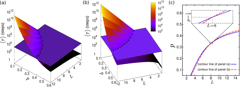
Figure 5: Mean first-passage time via Eq. (5) versus the effective tendency $p$ to jump toward the target and the tree extent $L$ at (a) $m{=}1$, $q{=}\frac{1}{3}$ and (b) $m{=}0.05$, $q{=}0.8$. The flat (constant MFPT) planes correspond to the MFPTs measured by tracer particles in experiments (chosen to be $\langle\tau\rangle{\simeq}1500$ and $15000$ steps in panels (a) and (b), respectively). The dashed line marks the intersection of the two surfaces, i.e. the contour line along which the MFPT equals the measured value. (c) Intersected contour lines in the $(L,p)$ phase space. Inset: A zoomed view of the same plot near the intersection, which determines the unknown values of the structural parameters.

By extracting $\alpha$ for other values of the structural parameters $L$ and $p$, we find that $\alpha$ scales exponentially with the extent of the tree $L$ if $p{<}\frac{1}{2}$. However, a crossover to power-law scaling occurs for $p{\geq}\frac{1}{2}$, as shown in Figs. 4(a),(b). The overall shape of $F(\tau)$ exhibits a plateau or even develops a peak at short times in general. The characteristic time to converge to the exponential tail behavior reduces with decreasing $p$, such that the entire distribution $F(\tau)$ follows an exponential form in the limit $p{\rightarrow}0$. Consequently, the mean value of $F(\tau)$ (i.e. the MFPT $\langle\tau\rangle$) is inversely related to the slope $\alpha$ at small values of $p$, as expected for exponential distributions. With increasing $p$, the form of $F(\tau)$ changes, thus, the deviations from $\alpha{=}\frac{1}{\langle\tau\rangle}$ grow, as shown in Fig. 4(c).

The MFPT can be calculated as $\langle\tau\rangle=z\frac{d}{dz}F(z)\Bigr{|}_{z{\rightarrow}1}$. We expand Eq. (3) around $z{=}1$ up to first order terms, as $F(z){\sim}F(z)\Bigr{|}_{z{\rightarrow}1}{+}(z{-}1)\frac{d}{dz}F(z)\Bigr{|}_{z{\rightarrow}1}{+}\mathcal{O}\Big{(}(z{-}1)^{2}\Big{)}$, and obtain the following exact expression for the MFPT

$$\langle\tau\rangle{=}\begin{cases}\displaystyle\frac{(m{-}q)L{+}q\,L^{2}}{m\,q},&p{=}\frac{1}{2},\vspace{1mm}\\ \displaystyle\frac{L}{m\,(2p{-}1)}{+}\frac{p\,q{-}p\,m\,(2p{-}1)}{m\,q\,(2p{-}1)^{2}}\Big{(}(\frac{1}{p}{-}1)\!^{{}^{L}}\!\!{-}1\Big{)},&p{\neq}\frac{1}{2}.\end{cases}$$ (5)

The MFPT diverges in the limit $L{\rightarrow}\infty$ as expected for infinite structures. It can be also seen that the MFPT scales linearly (exponentially) with the extent of the tree $L$ in the limit $p{\rightarrow}1$ ($p{\rightarrow}0$), as the exponential term on the right-hand side of Eq. (5) vanishes (dominates). In the absence of waiting ($m{=}1$) and assuming that the reflection probability $q$ at the leaves equals the hopping probability $p$ toward the root at the bulk nodes ($q{=}p$), Eq. (5) for $p{\neq}\frac{1}{2}$ reduces to Eq. (1). It is also notable that the total number of nodes $N$ in a regular tree is given as $N{=}2^{L}$. Thus, the first (last) term of $\langle\tau\rangle$ for $p{\neq}\frac{1}{2}$ grows logarithmically (linearly) with the number of nodes Wu12 .

According to Eq. (5), the MFPT of an intermittent random walk to travel from the leaves to the root depends on the set of parameters $\{L,p,m,q\}$. Let us suppose that the intrinsic dynamics of the lazy random walkers, characterized by $m$ and $q$ parameters, can be tuned before they start to explore the structure as tracer particles. For a given set of $m$ and $q$, one obtains a surface in the $(L,p,\langle\tau\rangle)$ phase space via Eq. (5). The intersection of this surface with a flat plane representing the measured MFPT results in an iso-MFPT contour line in the $(L,p)$ plane. An example is presented in Fig. 5(a) for $m{=}1$ and $q{=}\frac{1}{3}$, assuming that the measured MFPT is $\langle\tau\rangle{\simeq}1500$ steps. By repeating this procedure for a different set of $m$ and $q$ (with a different $\frac{m}{q}$ ratio), we can obtain another contour line in the $(L,p)$ plane which intersects the previous one and, thus, uniquely determines the structure (i.e. $L$ and $p$ parameters). Fig. 5(b) shows an example, where new parameter values $m{=}0.05$ and $q{=}0.8$ are chosen. Assuming that the measured MFPT for this lazy random walker is $\langle\tau\rangle{\simeq}15000$ steps, we obtain the second contour line. The intersected contour lines in Fig. 5(c) reveal that the unknown tree has the extent $L{=}8$ and the effective tendency $p{\simeq}\frac{1}{3}$ to move toward the root (corresponding to the node degree $k{=}3$ in the case of uniform links). Therefore, having access to the MFPTs of lazy random walkers provides sufficient information to unravel the structure.

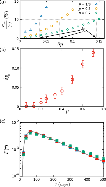
Figure 6: (a) The standard deviation of the MFPT in simulations, scaled by the analytical prediction for $\langle\tau\rangle$ via Eq. (5), in terms of the variation range $\delta p$ around its mean value $p$ at $L{=}10$ and $m{=}q{=}1$. The results are shown for three different values of $p$. The horizontal dashed line corresponds to $10\%$ error in the measured MFPT in simulations compared to the analytical prediction. (b) The critical variation range of the effective tendency $\delta p_{c}$ (which causes $10\%$ differences between simulation and theory) in terms of $p$. (c) The FPT distribution obtained via Eq. (3) (solid line) or simulations with $\delta p{\sim}0.02$ (blue symbols), $0.04$ (red symbols), and $0.10$ (green symbols). The results of uniform probability distributions of $p$ (full triangles) are compared to those obtained from normal distributions (open squares)

.

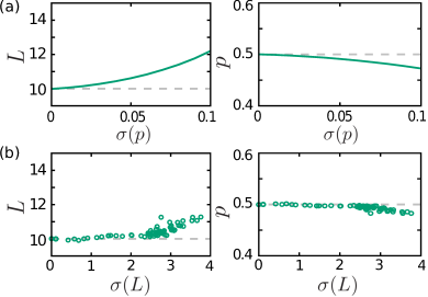
Figure 7: The estimated values of the structural parameters $L$ and $p$ versus the structural disorder characterized by the variance of the parameter (a) $p$ and (b) $L$. The horizontal dashed lines indicate the actual parameter values. The parameter values (unless varied) are taken to be $L{=}10$ and $p{=}m{=}q{=}\frac{1}{2}$. Each data point in panel (b) represents the result for a given static tree with a stochastic irregular branching pattern.

IV Disordered networks and experimental uncertainties

In derivation of the MFPT in the previous section, we considered a regular tree with the same tree extent along all branches and the same effective tendency to jump toward the target at every node. However, the real or virtual tree structures of interest are disordered. Particularly, heterogeneity in the degree of the nodes or in the capacity of the links has been widely studied in the context of complex networks. If the degree of the nodes or the weight of the links follow probability distributions, the effective tendency to move toward the target varies from node to node. The question arises of how far our analytical predictions for a regular tree remain valid when the network connectivity pattern becomes more and more diverse. To answer this question, we compare the analytical result of the MFPT for the constant $p$ across the tree, via Eq. (5), with the Monte Carlo simulation results where $p$ dynamically fluctuates at each node around the mean global value. Before each jump, we assign a new value to the effective tendency to move toward the target, which is randomly taken from a uniform probability distribution in the interval $[p{-}\delta p,p{+}\delta p]$.

Fig. 6(a) shows that the deviations of the MFPT from the analytical expression (5) grow with increasing the variation range $\delta p$. It can be seen that the significance of the impact on the MFPTs depends on the mean value of $p$. The higher the tendency to jump toward the target node, the more robust the analytical predictions become. For comparison, we define an upper threshold of $10\%$ deviations of the MFPT from the theory and measure the critical value $\delta p_{c}$ for the variation range of the parameter $p$ in simulations, at which the fluctuations of the MFPT reach the $10\%$ threshold. As shown in Fig. 6(b), broader fluctuations in $p$ can be tolerated with increasing $p$. For example, even a broad range of $15\%$ variations of $p$ around the mean value $p{=}0.7$ does not cause $10\%$ deviations in the measured MFPT from the predicted value. In regular trees with node degree $k{\gg}1$, $p{\rightarrow}0$ and the analytical predictions are only applicable in the limit of small variations in the degree of the nodes across the tree. As mentioned above, we have chosen a uniform distribution for $p$. In order to clarify whether the form of the probability distribution influences the MFPT results, we compare uniform and normal distributions of $p$ with the same mean and variance in Fig. 6(c). The mean value is fixed at $\langle p\rangle{=}\frac{1}{2}$ and a few examples for $\delta p$ have been examined. It can be seen that the differences between the FPT distributions are negligible when the first two moments of the distributions of the parameter $p$ are equal.

Next we investigate the influence of the structural disorder on the estimation of $L$ and $p$, as the main objective of the present study. We perform simulations where either $p$ or $L$ is allowed to fluctuate around its mean value. Let us first consider a tree with $L{=}10$ and allow $p$ to dynamically vary around $\langle p\rangle{=}\frac{1}{2}$ in Monte Carlo simulations through the procedure which was previously explained in this section. By obtaining the MFPT from simulations and inserting it in Eq. (5), one can predict the structural parameters for a given standard deviation $\sigma(p)$. Assuming that one of the structural parameters $L$ or $p$ is known, we estimate the other one via Eq. (5) and compare it to its actual value in Fig. 7(a). The deviation from the analytical prediction grows with increasing $\sigma(p)$, however, the effect is less pronounced for estimation of $p$ compared to $L$. We also note that the deviations are smaller for higher values of $\langle p\rangle$ (not shown). Our theoretical approach is thus applicable to treelike networks with moderate disorder in their connectivity pattern. We remind that according to Eq. (5) the MFPT approaches a linear scaling when $p{\rightarrow}1$, while it grows almost exponentially when $p$ decreases toward zero. Therefore, it is expected that the variation of $p$ around a mean value in the linear regime ($\langle p\rangle{>}\frac{1}{2}$) induces less deviations in the measured MFPTs, leading to a more accurate estimation of the structural parameters. On the other hand, fluctuations of $p$ around a mean value in the exponential regime ($\langle p\rangle{<}\frac{1}{2}$) causes an overestimation of the MFPT on average, which increases the errors of the estimated structural parameters.

In order to study disorder in the extent of the tree, we generate static irregular trees with $\langle L\rangle{=}10$ and standard deviation $\sigma(L)$ in the following way: we randomly allow the nodes to have their child nodes in a hierarchical manner starting from the root node. The procedure continues until the average extent of the tree reaches $\langle L\rangle{=}10$. In Fig. 7(b), we have presented the results for a tree with $p{=}\frac{1}{2}$ and for $m{=}q{=}\frac{1}{2}$ as an example. The deviations from analytical predictions remain below $10\,\%$ even in considerably heterogeneous trees with $\frac{\sigma(L)}{\langle L\rangle}{\approx}40\,\%$.

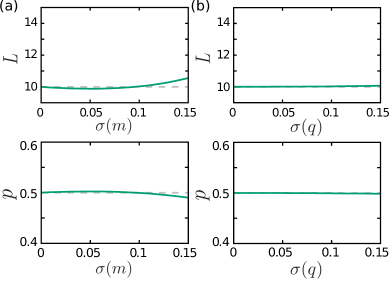
Figure 8: The estimated values of the structural parameters $L$ and $p$ versus the experimental uncertainty characterized by the variance of the parameter (a) $m$ and (b) $q$. The horizontal dashed lines indicate the actual parameter values. The parameter values (unless varied) are taken to be $L{=}10$ and $p{=}m{=}q{=}\frac{1}{2}$. The mean values of the variable parameters are $\langle m\rangle{=}\frac{1}{2}$ and $\langle q\rangle{=}\frac{1}{2}$ in panels (a) and (b), respectively.

In addition to disorder in the structure of the network, one may introduce uncertainty in tunning the experimental parameters $m$ and $q$. For example, intermittent random walks induced by random trapping and release in cages or by stochastic temporal absorption along the path lead to statistical errors for the resulting waiting probabilities $m$ and $q$. In order to assess the robustness of our analytical estimation of $L$ and $p$ in the presence of experimental uncertainties, we perform simulations where the structure is regular but the parameters $m$ and $q$ fluctuate around their mean values. In each of the Monte Carlo simulations, we vary only one of the experimental parameters $m$ or $q$ while the other one is fixed at its mean value. A new value is assigned to the variable parameter at each random walk step, which is randomly taken from a uniform distribution with standard deviation $\sigma(m)$ or $\sigma(q)$. For a given fluctuation range [either $\sigma(m)$ or $\sigma(q)$], we obtain the MFPT from simulations. Next, we insert the resulting MFPT (as well as $\langle m\rangle$, $\langle q\rangle$, and one of the structural parameters $L$ or $p$) in Eq. (5) to predict the remaining structural parameter. In Fig. 8, we compare the analytical estimations with the actual values to demonstrate the impact of uncertainty in the experimental parameters on the prediction of $L$ and $p$. It can be seen that the predicted values of $p$ or $L$ insignificantly deviate from the actual values for moderate (even up to $15\%$) experimental uncertainties.

V Discussion and conclusion

We presented an analytical framework to calculate the first-passage properties of intermittent random walks on treelike networks in terms of the waiting probabilities at the bulk nodes and leaves as well as the structural properties of the network such as its connectivity and extent. We proposed simple measurements of the mean-first-passage times of tracer particles entering the tree at the leaves and exiting from the root, to uniquely determine the structural properties. In regular trees, having access to the MFPT for only two different sets of waiting probabilities would be enough to unravel the structure. The idea of tuning the waiting probabilities of the random walkers to unravel the structure can be extended to other intrinsic dynamic properties such as the persistency of the walker Sadjadi15 ; Newby09 . Persistent random walkers can be employed to explore the structure of 1D domains and obtain their length and the effective bias to hop toward the target, even though assigning a persistency to the particle dynamics on a network topology is not well defined in general. Calculating the higher moments of the FPT distribution is another possibility. Since the $i$-th moment $\langle\tau^{i}\rangle=(z\frac{d}{dz})^{i}F(z)\Bigr{|}_{z{\rightarrow}1}$ can be straightforwardly obtained, having access to the first two moments of the FPT distribution also enables one to uniquely determine the structure via our analytical framework. However, the resulting set of equations may be redundant in special cases and it is considerably more difficult to evaluate variance or higher moments of the FPT distribution in experiments.

We addressed the validity range of the analytical predictions in networks with diverse connectivity patterns or heterogeneous branching morphologies. In the presence of disorder in the structural parameters $L$ and $p$ or uncertainty in the experimental parameters $m$ and $q$, even more measurements are required to determine the MFPT itself with a given accuracy. Therefore, it is naturally expected that the evaluation of the second moment of the FPT distribution with a given accuracy would be extremely time consuming in such cases. The advantage of considering intermittent random walks is that equipping particles with different diffusivity in experiments is possible, which makes our proposed measurements feasible in practice. The final remark is that the results obtained in this study are equivalently applicable to ordinary random walks on treelike structures which induce temporal absorption along the path or at the dead ends. A particularly relevant example is the transport in neuronal dendrites in the presence of biochemical cages along the dendritic tube.

- (1) D. ben-Avraham and S. Havlin, Diffusion and Reactions in Fractals and Disordered Systems (Cambridge University Press, Cambridge, 2000).
- (2) M. Felici, M. Filoche, and B. Sapoval, Phys. Re. Lett. 92, 068101 (2004).
- (3) Z. Sadjadi, M. F. Miri, M. R. Shaebani, and S. Nakhaee, Phys. Rev. E 78, 031121 (2008).
- (4) E. Agliari, A. Blumen, and O. Mülken, J. Phys. A 41, 445301 (2008).
- (5) E. Agliari and D. Cassi, First-Passage Phenomena and Their Applications (World Scientific, Singapore, 2014), pp. 96-121.
- (6) P. Tierno and M. R. Shaebani, Soft Matter 12, 3398 (2016).
- (7) M. Kac, Am. Math. Mon. 73, 1 (1966).
- (8) P. P. Mitra, P. N. Sen, L. M. Schwartz, and P. Le Doussal, Phys. Re. Lett. 68, 3555 (1992).
- (9) R. W. Mair, G. P. Wong, D. Hoffmann, M. D. Hürlimann, S. Patz, L. M. Schwartz, and R. L. Walsworth, Phys. Re. Lett. 83, 3324 (1999).
- (10) R. Krishna, J. Phys. Chem. C 113, 19756 (2009).
- (11) F. F. Chen and Y. S. Yang, Modelling Simul. Mater. Sci. Eng. 20, 045005 (2012).
- (12) D. J. Durian, D. A. Weitz, and D. J. Pine, Science 252, 686 (1991).
- (13) G. Maret, Curr. Opin. Colloid Interface Sci. 2, 251 (1997).
- (14) C. Cooper, T. Radzik, and Y. Siantos, Internet Mathematics 12, 221, 2016.
- (15) E. Agliari, R. Burioni, D. Cassi, and F. M. Neri, Theor. Chem. Acc. 118, 855 (2007).
- (16) V. Sood and P. Grassberger, Phys. Rev. Lett. 99, 098701 (2007).
- (17) E. Helfand and D. S. Pearson, J. Chem. Phys. 79, 2054 (1983).
- (18) B. Wu, Y. Lin, Z. Zhang, and G. Chen, J. Chem. Phys. 137, 044903 (2012).
- (19) D.-J. Heijs, V. A. Malyshev, and J. Knoester, J. Chem. Phys. 121, 4884 (2004).
- (20) D. Katsoulis, P. Argyrakis, A. Pimenov, and A. Vitukhnovsky, Chem. Phys. 275, 261 (2002).
- (21) P. Argyrakis and R. Kopelman, Chem. Phys. 261, 391 (2000).
- (22) N. Spruston, Nat. Rev. Neurosci. 9, 206 (2008).
- (23) H. Hering and M. Sheng, Nat. Rev. Neurosci. 2, 880 (2001).
- (24) R. Jose, L. Santen, and M. R. Shaebani, Biophys. J. (2018).
- (25) V. Fleury, J.-F. Gouyet, and M. Leonetti, Branching in nature: dynamics and morphogenesis of branching structures, from cell to river networks (Springer-Verlag, Berlin, 2001).
- (26) G. Szabó, M. Alava, and J. Kertész, Phys. Rev. E 66, 026101 (2002).
- (27) B. Bollobás and O. Riordan, Phys. Rev. E 69, 036114 (2004).
- (28) S. Redner, A Guide to first-passage processes (Cambridge University Press, New York, 2001).
- (29) B. D. Hughes and M. Sahimi, J. Stat. Phys. 29, 781 (1982).
- (30) C. Monthus and C. texier, J. Phys. A 29, 2399 (1996).
- (31) D. Cassi, Europhys. Lett. 9, 627 (1989).
- (32) S. H. Yook, H. Jeong, A.-L. Barabási, and Y. Tu, Phys. Rev. Lett. 86, 5835 (2001).
- (33) E. Almaas, P. L. Krapivsky, and S. Redner, Phys. Rev. E 71, 036124 (2005).
- (34) A. Barrat, M. Barthélemy, R. Pastor-Satorras, and A. Vespignani, Proc. Natl. Acad. Sci. U.S.A. 101, 3747 (2004).
- (35) A. E. Krause, K. A. Frank, D. M. Mason, R. E. Ulanowicz, and W. W. Taylor, Nature 426, 282 (2003).
- (36) M. Khantha and V. Balakrishnan, Pramana 21, 111 (1983).
- (37) L. Skarpalezos, A. Kittas, P. Argyrakis, R. Cohen, and S. Havlin, Phys. Rev. E 88, 012817 (2013).
- (38) R. Garcia-Pelayo, Physica A 384, 143 (2007).
- (39) N. Pottier, Physica A 230, 563 (1996).
- (40) G. H. Weiss, Physica A 311, 381 (2002).
- (41) O. Benichou, A. M. Cazabat, A. Lemarchand, M. Moreau, and G. Oshanin, J. Stat. Phys. 97, 351 (1999).
- (42) V. Mehra and P. Grassberger, Physica D 168, 244 (2002).
- (43) M. R. Shaebani, Z. Sadjadi, I. M. Sokolov, H. Rieger, and L. Santen, Phys. Rev. E. 90, 030701 (2014).
- (44) J. Masoliver, K. Lindenberg, and G. H. Weiss, Physica A 157, 891 (1989).
- (45) A. E. Hafner, L. Santen, H. Rieger, and M. R. Shaebani, Sci. Rep. 6, 37162 (2016).
- (46) Y. Kantor and M. Kardar, Phys. Rev. E 76, 061121 (2007).
- (47) T. Huisinga, R. Barlovic, W. Knospe, A. Schadschneider, and M. Schreckenberg, Physica A 294, 249 (2001).
- (48) A. D. Kachhvah and N. Gupte, Phys. Rev. E 86, 026101 (2012).
- (49) Z. Sadjadi, M. R. Shaebani, H. Rieger, and L. Santen, Phys. Rev. E. 91, 062715 (2015).
- (50) M. Newby and P. C. Bressloff, Phys. Rev. E. 80, 021913 (2009).