Random Phase Approximation in Projected Oscillator Orbitals.

Résumé

The projected oscillator orbitals (pOOs) are localized virtual orbitals constructed by multiplying localized occupied orbitals by harmonics. Following a recent paper by Mussard and ÁngyánMussard (2015), further developments of projected oscillator orbitals are shown, notably the equations for pOOs of general order as well as their overlaps are derived. The performance of these localized virtual orbitals is demonstrated up to third order. It is found that a good fraction of the aug-cc-pVQZ RPA correlation energy is recovered by use of a smaller number of pOOs. This is especially true where considering only the long-range correlation energy, which is important for the description of London dispersion forces.

Introduction

In the context of density functional approximations, the functionals from the so-called fifth rung of the Jacob’s ladder not only use the density, its gradient, and a set of occupied orbitals but require also a priori the knowledge of the set of virtual orbitals. Such methods have the obvious drawback that the size of the virtual orbital space can be very large.

A solution often used to keep the size of matrices in reasonable limits employs an auxiliary basis set to expand the occupied-virtual products. Such approaches are known in quantum chemistry as resolution of identity Eichkorn et al. (1995) or density-fitting Whitten (1973); Roeggen and Johansen (2008) methods and similar advantages can be found by use of Cholesky decomposition Beebe and Linderberg (1977) techniques.

Further gain can be achieved by local correlation methods, which take advantage of the locality of purposefully made orbitals to reduce the number of significant terms to calculate in a given method. Hence, both the localization of orbitalsHøyvik et al. (2012); Aqui ; Yang2011a ; Brani ; Zhang ; Subot2005 ; Hess2016 ; Maynau and the derivation of local correlation methodsYang2011 ; Yang2012 ; Christ ; Subot2006 ; Kallay ; Hess2017 have lately been an active area of research.

In the present work it is shown that accurate random phase approximation (RPA) energies can be evaluated with approximations which avoid any explicit reference to virtual orbitals and involve quantities that are computable from occupied orbitals alone, much like what was shown by Surján for MP2Surján (2005). The strategy followed here uses localized virtual orbitals called the projected oscillator orbitals (pOOs)Mussard (2015), in the spirit of the projected atomic orbitals techniques Pulay (1983); Pulay and Saebø (1986); Boughton and Pulay (1993).

In a fairly recent paperMussard (2015), we showed that the pOOs, an original idea by Foster and BoysFoster and Boys (1960a, b); Boys (1966), could be used in the context of the RPA equations. The core idea behind the pOOs is to construct a set of virtual orbitals directly from a set of occupied localized orbitals (LMOs) by multiplying them with solid spherical harmonics. The orthogonality of these oscillator orbitals with the occupied space is ensured by projection to obtain the projected oscillator orbitals. The pOOs are non-orthogonal among each other which is a source of some complications, although only to the same extent and in the same manner as in the case of the projected atomic orbitals, and the work that has been done over the years in the context of local correlation methods using projected atomic orbitalsKnowles et al. (2000) can be used. As mentioned in another paperMussard (2015), the pOOs show similarities with other worksKirkwood (1932); Pople and Schofield (1957); Karplus and Kolker (1963a, b); Rivail and Cartier (1978, 1979); Sadlej and Jaszunski (1971).

The main interest of this paper is not to reproduce the full correlation energy with high numerical precision, but only a well-defined part of it, namely the long-range dynamical correlation energy which is usually responsible for the London dispersion forces. It is indeed now well-documented that most of the conventional density functional calculations in the Kohn-Sham framework are unable to grasp the physics of these long-range forces, unless special corrections are added to the total energyJohnson and Becke (2005); Johnson et al. (2009); Grimme et al. (2010); Grimme (2011); Tkatchenko and Scheffler (2009); DiStasio et al. (2014); Reilly and Tkatchenko (2015). On the other hand it has been demonstrated in earlier worksToulouse et al. (2009); Zhu et al. (2010); Ángyán et al. (2011); Toulouse et al. (2011) that the essential physical ingredients of London dispersion forces are contained in the range-separated hybrid RPA method, where the short-range correlation effects are described within a density functional approximation and the long-range exchange and correlation are handled at the long-range Hartree-Fock and long-range RPA levels. The range-separated hybrid method has the additional advantage of showing a more favorable convergance with basis set sizebasisconv . Note that the use of localized orbitals for dispersion energy calculations has already been proposed since the early works on local correlation methods Kapuy and Kozmutza (1991); Saebø et al. (1993); Hetzer et al. (1998); Usvyat et al. (2007); Chermak et al. (2012).

In the following, new derivations of the projected oscillator orbitals framework are presented as well as a very brief recall of the local formulation of the random phase approximation equations before showing the performance on full-range and long-range correlation energies. Detailed derivations are provided in the Appendix when needed.

Projected Oscillator Orbitals

A set of oscillator orbitals (OOs) is produced by multiplying a set of localized molecular orbitals (LMOs) $\{|i\rangle\}$ by solid spherical harmonics centered on the barycenter $\mathbf{D}^{i}$ of the LMOs (here for the first order solid spherical harmonic):

$$|\text{OO}\rangle=(\hat{r}_{\alpha}-D^{i}_{\alpha})|i\rangle$$ (1)

where $\hat{r}_{\alpha}$ is the $\alpha=x,y,z$ component of the position operator. The set of localized virtual orbitals $\{|i_{\alpha}\rangle\}$ that are the projected oscillator orbitals (pOOs) is constructed by projecting the oscillator orbitals out of the occupied space:

$$|\text{pOO}\rangle=\hat{P}\,(\hat{r}_{\alpha}-D^{i}_{\alpha})|i\rangle\doteq|i_{\alpha}\rangle$$ (2)

where $\hat{P}=(\hat{1}-\sum|k\rangle\langle k|)$ and where the composite index “$i_{\alpha}$” refers to a pOO generated from the $i$-th LMO by using the $\hat{r}_{\alpha}$ harmonic. The pOOs are not orthogonal among each other, and have an overlap (here again between the first order pOOs):

$$S_{i_{\alpha}j_{\beta}}=\langle i|\hat{r}_{\alpha}\hat{P}\,\hat{r}_{\beta}|j\rangle =\langle i|\hat{r}_{\alpha}\hat{r}_{\beta}|j\rangle$$

$$\quad-\sum_{k}^{N_{\text{LMO}}}\langle i|\hat{r}_{\alpha}|k\rangle\langle k|\hat{r}_{\beta}|j\rangle$$ (3)

where $N_{\text{LMO}}$ is the number of (localized) occupied orbitals.

In Eq. (2), the tail emerging from the projection term $\sum|k\rangle\langle k|\hat{r}_{\alpha}|i\rangle$ obviously damages the locality of the pOOs. The Foster-Boys localization criterion for the LMOsFoster and Boys (1960a); Boys (1966) precisely ensures that the sum of the off-diagonal elements of the $\hat{r}_{\alpha}$ operators taken between the occupied orbitals is minimizedResta (2006). Hence the pOOs are optimally localized when used in conjunction with LMOs obtained by use of the Foster-Boys criterion.

The virtual pOOs have by design a nodal surface intersecting the occupied orbital centroid and coinciding with the region of the highest electron density of the occupied orbital: this ensures an optimal description of the correlation.

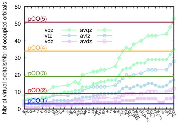
Figure 1: Number of virtual orbitals in terms of multiples of the number of occupied orbitals for the atoms and molecules considered in this paper. In filled symbols are the cc-pVXZ basis sets, denoted “vdz”, “vtz” and “vqz”, and in shallow symbols are the aug-cc-pVXZ, denoted “avdz”, “avtz” and “avqz”. The sets of pOOs up to a given order each yield a constant number of virtual orbitals in terms of multiples of the number of occupied orbitals, shown by the horizontal lines.

Higher order pOOs

Higher order pOOs that have further nodes can be obtained in a similar way, using higher order polynomials. A pOO of general order $n$ hence reads:

$$|i_{\alpha\dots\eta}\rangle=\hat{P}\,(\hat{r}_{\alpha}-D^{i}_{\alpha})\dots(\hat{r}_{\eta}-D^{i}_{\eta})|i\rangle$$ (4)

It can be shown (see Appendix) that pOOs can be written as a function of pOOs of lower order:

$$|i_{\alpha\dots\eta}\rangle=\hat{P}\,\hat{r}_{\alpha}\dots\hat{r}_{\eta}|i\rangle-\sum_{k=1}^{n-1}\underbrace{\vphantom{|K\rangle}D^{i}\dots D^{i}}_{n-k}\underbrace{|K\rangle}_{\begin{subarray}{c}\text{pOO of}\\ \text{order }k\end{subarray}}$$ (5)

In this equation, every term of order $k$ in the sum is actually replicated ${n\choose k}$ times, each time assigning a different set of $k$ indices to the pOO $|K\rangle$ and the remaining indices to the vector component $\mathbf{D}^{i}$. This explains why the terms in the sum are not written with their indices, and might be made clearer with an example, found in the Appendix. As a result of Eq. (5), the overlaps involving any order of pOOs are functions of lower order overlaps:

$$\langle N|M\rangle =\langle i|\underbrace{\hat{r}\dots\hat{r}}_{n}\hat{P}\,\underbrace{\hat{r}\dots\hat{r}}_{m}|j\rangle$$

$$-\underset{k+l\neq n+m}{\sum_{k=1}^{n}\sum_{l=1}^{m}}\underbrace{D^{i}\dots D^{i}}_{n-k}\langle K|L\rangle\underbrace{D^{j}\dots D^{j}}_{m-l}$$ (6)

where again the terms of the sum are replicated ${n\choose k}{m\choose l}$ times with a different set of $k$ indices assigned to the pOO $\langle K|$, a different set of $l$ indices assigned to the pOO $|L\rangle$, and the remaining indices to the vectors $\mathbf{D}^{i}$ and $\mathbf{D}^{j}$. The pOOs of a given order $n$ and all equations involving those pOOs hence only need ingredients (overlap, etc…) already constructed for lower order pOOs plus at most the matrix elements of the multipole operator of order $2n$.

Size of the virtual orbital space

Table 1: Number of virtual orbitals generated at and up to a given order of harmonics used.

order of the pOOs	figurate number	number of pOOs generated	cumulant number of pOOs
1	$\displaystyle{3\choose 1}$	$\phantom{1}3\times N_{\text{LMO}}$	$\phantom{1}3\times N_{\text{LMO}}$
2	$\displaystyle{4\choose 2}$	$\phantom{1}6\times N_{\text{LMO}}$	$\phantom{1}9\times N_{\text{LMO}}$
3	$\displaystyle{5\choose 3}$	$10\times N_{\text{LMO}}$	$19\times N_{\text{LMO}}$
4	$\displaystyle{6\choose 4}$	$15\times N_{\text{LMO}}$	$34\times N_{\text{LMO}}$
5	$\displaystyle{7\choose 5}$	$21\times N_{\text{LMO}}$	$51\times N_{\text{LMO}}$

Figure 2: Examples of pOOs generated from the oxygen lone pair of the formaldehyde (left panels) by applying first-, second- and third order harmonics (second, third and last panels). The first row shows contour taken on the blue plane in the sketch molecule on the left, the second row shows contour taken on the red plane.

The number of first order pOOs generated is $3.N_{\text{LMO}}$ (the $x$, $y$ and $z$ pOOs constructed for each LMO). In terms of multiples of the number of LMOs, the number of pOOs generated at each order $n$ of spherical harmonics used is given by a figurate number (linear number for first order, triangular number for second order, tetrahedral number for third order, etc…), which simply corresponds to the number of unique $n$-tuplets that can be made with $x,y,z$

$$P(n)=\frac{1}{2}(n+1)(n+2)={n+2\choose n}$$ (7)

This is summed-up in Table 1, which also shows the cummulated number of pOOs generated up to order $n$ for the first 5 orders. As comparison, Figure 1 shows the number of virtual orbital generated by the widely used Dunning basis sets cc-pVDZ, cc-pVTZ, cc-pVQZ, aug-cc-pVDZ, aug-cc-pVTZ, and aug-cc-pVQZ for the atoms and molecules on which the correlation energy are calculated in this paper (those are taken from the set of the small systems compiled by Tkatchenko and SchefflerTkatchenko and Scheffler (2009); Toulouse et al. (2013)). This shows that for example the set of pOOs up to third order yields a size of virtual space greater than the one generated by the cc-pVTZ and on par with the one generated by aug-cc-pVTZ.

Local RPA equations

The random phase approximation can be formulated in a number of different waysÁngyán et al. (2011); Toulouse et al. (2011); urpa ; diel ; frac , but in a local formulation of the “ring coupled-cluster double” (rCCD), the RPA correlation energy can be given by a sum over (localized) pair contributions:

$$E_{c}=\frac{1}{2}\text{Tr}\left(\mathbf{K}^{ij}\mathbf{T}^{ji}\right)$$ (8)

where the amplitudes $\mathbf{T}$ are found by solving the Riccati equations $\mathbf{R}^{ij}=\mathbf{0}$, where:

$$\mathbf{R}^{ij} =\mathbf{B}^{ij}+\mathbf{A}^{im}\mathbf{T}^{mj}\mathbf{S}+\mathbf{S}\mathbf{T}^{im}\mathbf{A}^{mj}$$

$$\quad+\mathbf{S}\mathbf{T}^{im}\mathbf{B}^{mn}\mathbf{T}^{nj}\mathbf{S}$$ (9)

where the matrices are written in the LMOs/pOOs basis:

$$A^{ij}_{k_{\alpha}l_{\beta}} =\langle ij|k_{\alpha}l_{\beta}\rangle-\langle k_{\alpha}i|l_{\beta}j\rangle+\epsilon^{ij}_{k_{\alpha}l_{\beta}}$$

$$B^{ij}_{k_{\alpha}l_{\beta}} =\langle ij|k_{\alpha}l_{\beta}\rangle-\langle ij|l_{\beta}k_{\alpha}\rangle$$

$$\epsilon^{ij}_{k_{\alpha}l_{\beta}} =\delta_{ij}f_{k_{\alpha}l_{\beta}}-S_{k_{\alpha}l_{\beta}}f_{ij}$$ (10)

where $\mathbf{f}$ is the Fock matrix in LMOs/pOOs basis and the two-body integrals between LMOs and pOOs are in physicist’s notation. The Riccati equations are solved iteratively in a pseudo-canonical basis; see our original paperMussard (2015) for more detailed derivations and a detailed workflow in the appendix.

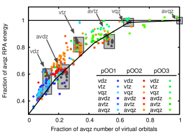
Figure 3: Results of calculations of the RPA correlation energies (left: full-range, right: long-range) of a small set of molecules. Each dot represents a result for one of those molecule, obtained with several different basis. The gray boxes gather the gray dots corresponding to reference results that are obtained with the unmodified cc-pVDZ, aug-cc-pVDZ, cc-pVTZ, aug-cc-pVTZ, cc-pVQZ and aug-cc-pVQZ basis sets (denoted as vdz, avdz, etc…). The color dots are the pOO results, with pOOs of first (second and third) order being in blue (red and green). Those pOOs can be obtained in the context of the different reference Dunning basis, hence the nuances of blue, red and green. The black line in both plots roughly connects the centers of the gray boxes.

Correlation energies

The performance of the pOOs is investigated for the calculation of the RPA correlation energies of a set of small moleculesTkatchenko and Scheffler (2009) already used in our original paperMussard (2015). Both post-HF calculations and range-separated hybrid calculations using the RSHPBE functional with a parameter $\mu=0.5$ are performed. The occupied orbitals obtained are localized, and the pOOs are generated before calculating either the full-range or the long-range RPA correlation energies.

All calculations were performed with a development version of the quantum chemical program package MolproWerner et al. (2010), where the construction of the pOOs up to third order has been implemented for the purpose of this paper, together with the corresponding overlaps.

Results of calculations using the cc-pVDZ, cc-pVTZ, cc-pVQZ as well as the aug-cc-pVDZ, aug-cc-pVTZ and aug-cc-pVQZ basis sets are shown. In practice, because of linear dependencies built in the pOOs (see briefly the workflow in the Appendix), the RPA equations are carried with an effective number of independant pseudo-canonical basis functionsMussard (2015) which can be lower than the multiple of the number of occupied orbitals mentioned in Table 1 and in Figure 1. The pertinent quantities to look at are hence the RPA correlation energies and the number of pseudo-canonical orbitals involved in the calculations. Figure 3 shows this in terms of the fractions of the aug-cc-pVQZ RPA correlation energies recovered as a function of the fractions of the aug-cc-pVQZ number of virtual orbitals involved in the calculations. On the left are shown post-HF results and on the right long-range RPA correlation energy results.

The RPA correlation energies obtained in each basis sets without the use of localized orbitals are shown in gray dots and gathered for clarity within gray boxes. The rest of the data (the RPA correlation energies obtained when using LMOs and pOOs) is shown in colored symbols. The results from pOOs obtained within a (aug-)cc-pVXZ basis are shown in diamonds (squares). The pOOs of first order are shown in shades of blue, of second order in shades of red and of third order in shades of green.

A first interesting result is that the performances of a given order of pOOs is not significantly changed by the basis used to construct them: pOOs will perform a certain way independently of the core basis set used (this is even more striking in the case of the long-range results, right of Figure 3). Furthermore, a positive finding is that the calculations involving pOOs recover a good portion of the targeted RPA correlation energies (full- or long-range) for the size of the virtual space involved. As a marker, the black line in the figure is drawn roughly between the center of the gray boxes holding the non-localized RPA energies, and shows the fraction of the aug-cc-pVQZ correlation energy recovered by smaller basis sets. The pOO results lie virtually systematically above that line, meaning the pOOs recover a larger portion of the targeted RPA energies than the basis set having similar numbers of virtual orbitals. Finally, as expected, the fraction of long-range RPA correlation energy recovered is significantly higher than the recovered portion of full-range correlation energy. This is a nice result, as the framework of pOOs was largely thought as a way to build approximations to model the London dispersion forces, as can be seen in our original paperMussard (2015).

Conclusion

It was shown that localized virtual orbitals can be constructed easily and systematically by multiplying localized occupied orbitals by harmonic functions of higher than first order. The size of the virtual space obtained is comparable to the size of that generated when using the Dunning basis sets, and the RPA correlation energies calculated with the pOO localized virtual orbitals are close to the energies without local approximations. Because of an interesting iterative feature emerging in the construction of the projected oscillator orbitals, it is easy to generate higher order pOO from generated lower order pOOs. A great number of additional approximation, developed in our original paperMussard (2015) in the context of first order projected oscillator orbitals, such that multipolar expansion to approximate the electron repulsion, spherical approximation, etc. could be applied in the future to the higher order pOOs derived here.

Appendix

Relations between pOOs

The natural expression for a pOO of order $n$ is given by the binomial theorem:

$$|i_{\alpha\dots\eta}\rangle =\hat{P}\,(\hat{r}_{\alpha}-D^{i}_{\alpha})\dots(\hat{r}_{\eta}-D^{i}_{\eta})|i\rangle=\sum_{k=1}^{n}A^{n}_{k}$$ (11)

where $A^{n}_{k}$ is defined for convenience:

$$A^{n}_{k}=(-1)^{n-k}\underbrace{(D^{i}\dots D^{i})}_{n-k}\hat{P}\,\underbrace{\vphantom{()}\hat{r}\dots\hat{r}}_{k}|i\rangle$$ (12)

and actually contains ${n\choose k}$ repetitions with different assignations of the indices $\alpha\dots\eta$. For each of those repetitions, a different set of $k$ indices among $\alpha\dots\eta$ is assigned to the $k$ position operators and the remaining indices are given to the vector components $D^{i}$. For example, consider a pOO $|i_{\alpha\beta\gamma}\rangle$ of order 3. The term $A^{3}_{1}$ will be:

$$A^{3}_{1}{}^{\phantom{\prime\prime}} =(D^{i}_{\alpha}D^{i}_{\beta})\hat{P}\,\hat{r}_{\gamma}|i\rangle$$

$$A^{3}_{1}{}^{\prime\phantom{\prime}} =(D^{i}_{\alpha}D^{i}_{\gamma})\hat{P}\,\hat{r}_{\beta}|i\rangle$$

$$A^{3}_{1}{}^{\prime\prime} =(D^{i}_{\beta}D^{i}_{\gamma})\hat{P}\,\hat{r}_{\alpha}|i\rangle$$

i.e. it contains ${3\choose 1}=3$ repetitions with different assignations of the indices $\alpha$, $\beta$ and $\gamma$.

We seek to prove Eq. (5), which amounts with the current notations to:

$$|i_{\alpha\dots\eta}\rangle=A^{n}_{n}-\sum_{k=1}^{n-1}\underbrace{\vphantom{|nk\rangle}D^{i}\dots D^{i}}_{n-k}\underbrace{|K\rangle}_{\begin{subarray}{c}\text{pOO of}\\ \text{order }k\end{subarray}}$$ (13)

where the same repetitions with different assignations of the indices $\alpha\dots\eta$ are found now for each terms of the sum. We begin by inserting in Eq. (13) the binomial expression of Eq. (11) for the pOO $|K\rangle$:

$$|i_{\alpha\dots\eta}\rangle =A^{n}_{n}-\sum_{k=1}^{n-1}\underbrace{(D^{i}\dots D^{i})}_{n-k}\sum_{m=1}^{k}A_{m}^{k}$$ (14)

where we can rewrite the term in the sums using:

$$\underbrace{(D^{i}\dots D^{i})}_{n-k}A_{m}^{k}$$

$$\quad=(-1)^{k-m}\underbrace{(D^{i}\dots D^{i})}_{n-k}\underbrace{(D^{i}\dots D^{i})}_{k-m}\hat{P}\,\underbrace{\vphantom{(}\hat{r}\dots\hat{r}}_{m}|i\rangle$$ (15)

$$\quad=(-1)^{k+n}A^{n}_{m}$$

This yields:

$$|i_{\alpha\dots\eta}\rangle =A^{n}_{n}+\sum_{k=1}^{n-1}\sum_{m=1}^{k}(-1)^{k+(n-1)}A^{n}_{m}$$

$$=A^{n}_{n}+\sum_{m=1}^{n-1}\left[\sum_{k=m}^{n-1}(-1)^{k+(n-1)}\right]A^{n}_{m}$$ (16)

where in the last line the double summation was simply rearranged (think of summations over lines versus over columns of a matrix whose columns are composed of $A^{n}_{m}$).

In terms of assignations of the indices $\alpha\dots\eta$, in Eq. (15) there is ${n\choose k}$ ways to assign indices to the first string of $n-k$ “$D^{i}$” and ${k\choose m}$ ways to assign indices to the second string of $k-m$ “$D^{i}$”. This hence becomes a combinatorial problem, and recovering Eq. (11) from Eq. (16) boils down to proving that:

$$\sum_{k=m}^{n-1}(-1)^{k+(n-1)}{n\choose k}{k\choose m}={n\choose m}$$ (17)

which should be the number of repeated occurences of the $A^{n}_{m}$ term with different indices in Eq. (16). This amounts to prove that:

$$\sum_{k=m}^{n-1}(-1)^{k+(n-1)}\frac{{n\choose k}{k\choose m}}{{n\choose m}}=1$$ (18)

where, manipulating the fraction, the expression to study is:

$$\sum_{k=m}^{n-1}(-1)^{k+(n-1)}{n-m\choose k-m}$$

$$=\sum_{k=m}^{n}(-1)^{k+(n-1)}{n-m\choose k-m}-(-1)^{-1}{n-m\choose n-m}$$

$$=\left\{\sum_{k^{\prime}=0}^{n-m}(-1)^{k^{\prime}}{n-m\choose k^{\prime}}\right\}(-1)^{n-m+1}+1$$

$$=1$$ (19)

where the first step consists simply in adding and substracting the $n$-th element of the sum, the second step is a change of the dummy index of the sum and the final step is a realization that the expression in curvy brackets is the binomial theorem for $(1+(-1))^{n-m}=0$. This proves Eq. (5).

Workflow

Although in our original paperMussard (2015) relations to construct all ingredients for the pOOs using solely data from the occupied space are presented (this is the purpose of the projected schemes), for the clarity of the proof-of-concept calculations in this paper, the $N_{\text{pOO}}\times N_{\text{vir}}$ matrix $\mathbf{V}$ to transform virtual orbitals to pOOs is introduced:

$$|i_{\alpha\dots\eta}\rangle=\sum_{a}^{N_{\text{vir}}}V_{i_{\alpha\dots\eta}a}|a\rangle$$ (20)

We assume here that the pOOs can be exanded in the virtual basis, i.e. that the pOO space is a subspace of the virtual space. This should be more rigourously checked in later work. For example, the $\mathbf{V}$ matrix corresponding to the first order pOO reads:

$$V^{(1)}_{i_{\alpha}a}=\langle i|\hat{r}_{\alpha}|a\rangle$$ (21)

and, given Eq. (5), repeated in the Appendix as Eq. (13), the $\mathbf{V}$ matrix corresponding to a $N$-th order pOO simply reads:

$$V^{(N)}_{i_{\alpha\dots\eta}a}=\langle i|\hat{r}_{\alpha}\dots\hat{r}_{\eta}|a\rangle-\sum_{k=1}^{n-1}\underbrace{\vphantom{V_{a}}D^{i}\dots D^{i}}_{n-k}\underbrace{V^{(K)}_{\dots a}}_{\begin{subarray}{c}\text{matrix for}\\ \text{order $k$}\\ \text{pOO}\end{subarray}}$$ (22)

The overlap between pOOs is $\mathbf{S}=\mathbf{V}\mathbf{V}^{\dagger}$ and the pseudo-canonical basis is obtained by solving the generalized eigenvalue equation

$$\mathbf{f}\mathbf{X}=\mathbf{S}\mathbf{X}\boldsymbol{\epsilon}$$ (23)

Because of linear dependencies built in the construction of the pOOs, the overlap matrix $\mathbf{S}$ is in general only positive semidefinite instead of positive definite. Hence the pseudo-canonical basis of effective size $N_{\text{eff}}\leq N_{\text{pOO}}$ can alternatively by found with the $N_{\text{pOO}}\times N_{\text{eff}}$ matrix $\mathbf{X}$ that similtaneously diagonalizes $\mathbf{f}$ and $\mathbf{S}$.

From these relations, one can then construct from the $N_{\text{AO}}\times N_{\text{vir}}$ tranformation matrix $\mathbf{C}$ the following sequential transformation matrices:

$$\underbrace{\mathbf{C}}_{\text{AO}\rightarrow\text{vir}}\rightarrow\underbrace{\mathbf{C}\mathbf{V}^{\dagger}}_{\text{AO}\rightarrow\text{pOO}}\rightarrow\underbrace{\mathbf{C}\mathbf{V}^{\dagger}\mathbf{X}}_{\text{AO}\rightarrow\text{pseudo-cano}}$$ (24)

to easily either try out the pOOs, draw them, or calculate energies.