On the Structure of Linear Dislocation Field Theory

Abstract

Uniqueness of solutions in the linear theory of non-singular dislocations, studied as a special case of plasticity theory, is examined. The status of the classical, singular Volterra dislocation problem as a limit of plasticity problems is illustrated by a specific example that clarifies the use of the plasticity formulation in the study of classical dislocation theory. Stationary, quasi-static, and dynamical problems for continuous dislocation distributions are investigated subject not only to standard boundary and initial conditions, but also to prescribed dislocation density. In particular, the dislocation density field can represent a single dislocation line.

It is only in the static and quasi-static traction boundary value problems that such data are sufficient for the unique determination of stress. In other quasi-static boundary value problems and problems involving moving dislocations, the plastic and elastic distortion tensors, total displacement, and stress are in general non-unique for specified dislocation density. The conclusions are confirmed by the example of a single screw dislocation.

AMS Classification: 74F99, 74G05, 74G30, 74H05, 74H25, 74M99.

Keywords: Dislocations. Volterra. Plasticity. Elasticity. Uniqueness.

1 Introduction

Dislocations in crystals are microstructural line defects that create ‘internal’ stress even in the absence of loads. Physical observation suggests that applied loads and mutual interaction cause dislocations to move and the body to become permanently deformed. The understanding and prediction of the internal stress field and accompanying permanent deformation due to large arrays of dislocations form part of the fundamental study of metal plasticity.

In an elastic body, a dislocation is defined in terms of the non-zero line integral of the elastic distortion around possibly time-dependent closed curves or circuits in the body. The elastic distortion itself is related to the stress through a linear constitutive assumption, while equilibrium requires the divergence of the stress to vanish in the absence of body-forces. When the dislocations are continuously distributed, Kröner [Krö81] uses Stokes’ theorem to derive the pointwise connection between the Curl operator of the elastic distortion and the dislocation density field. The connection is valid also for a single dislocation whether singular or not. Consequently, the elastic distortion is incompatible (i.e., is not the gradient of a vector field) in the theory of continuously distributed static dislocations, which contrasts with classical linear elasticity. Furthermore, it must be shown how the elastic distortion can be determined from the equilibrium equations and elastic incompatibility for given dislocation density and linear elastic response. Kröner adopts the dislocation density as data, but his proposed resolution of the problem determines only the symmetric part (the strain) of the elastic distortion. Willis [Wil67] observes that the boundary value problem with dislocation density as data in fact determines the complete elastic distortion (including rotation). Kröner also introduces a total (generally continuous) displacement field and defines the plastic distortion as the difference between the gradient of the displacement field and the elastic distortion. The approach is motivated by cut-and-weld operations [Nab67, Esh56, Esh57] used to describe dislocations.

Henceforth in this paper, the plasticity formulation, or theory, (of dislocations) involves the total displacement, stress, plastic distortion, and dislocation density fields. Stress is defined by linear dependence on the elastic distortion subject to the static or dynamic balance of forces. The complete representation of plasticity due to moving dislocations involves an evolution equation for the plastic distortion. This depends upon the stress state through a fundamental kinematical relation between the plastic distortion rate and both the dislocation density and stress-dependent velocity.

Thus, the stress and plastic distortion are intimately coupled. In this work, however, we simply determine the stress and displacement subject to data that includes various parts of the evolving plastic distortion field. It is of particular interest to investigate whether stress and displacement are uniquely determined when only the evolving dislocation density field is known. The topic is first encountered in the equilibrium traction boundary-value problem for which, as discussed later, the dislocation density is sufficient to uniquely determine the stress.

The classical theory of dislocations, developed in papers [Mic99a, Mic99b, Tim05, Wei01], is due to Volterra [Vol07] and does not deal with evolution. It regards a dislocation as the termination edge of a surface over which the total displacement is discontinuous by an amount that defines the Burgers vector. The traction remains continuous across the surface. (See also [Lov44, Nab67, HL82].) The classical theory is stated in multiply-connected regions excluding dislocation cores. In such a region, the displacement field of a dislocation may be viewed as a continuous multivalued ‘function.’ Alternatively, and more conveniently, it may be viewed as a discontinuous function with constant discontinuity across any surface whose removal from the (multiply-connected) region renders the latter simply-connected. On the simply-connected region obtained by the use of such ‘barriers’ or ‘cuts’, the displacement may be regarded as a single-valued continuous vector field, which nevertheless has different values at adjacent points on either side of each barrier.

The Volterra formulation contains singularities not necessarily present in the plasticity formulation. One task therefore is to reconcile the classical and plasticity formulations. As a first step, we explain how a single stationary Volterra dislocation line is the formal limit of a sequence of problems in plasticity theory. Plasticity theory is a physically more realistic non-singular description of moving dislocations and their fields. It avoids mathematical difficulties caused by nonlinearities in non-integrable fields that would otherwise appear in the full problem of evolution coupled to stress.

Apart from exploring the relevance of the plasticity formulation to an understanding of dislocations, whether according to Kröner’s or Volterra’s interpretation, another major consideration of this paper concerns uniqueness in the static and dynamic problems of the plasticity dislocation theory. Standard Cauchy initial conditions together with displacement, mixed, or traction boundary conditions are augmented by a prescribed dislocation density rather than the usual plastic distortion tensor. A previous contribution [Wil67] demonstrates that the stress and elastic distorsion to within a constant skew-symmetric tensor in the equilibrium traction boundary value problem on unbounded regions are unique subject to a prescribed dislocation density field. It is noteworthy that this approach dispenses entirely with the total displacement field. In contrast, it follows from Weingarten’s theorem that the displacement is not unique in the classical Volterra theory for a given dislocation distribution. Uniqueness, however, can be retrieved when the “seat of the dislocation” [Lov44], (the surface of displacement discontinuity) is additionally prescribed.

Time-dependent problems of plasticity in a body containing a possibly large number of moving dislocation lines are physically important. They become prohibitively complicated when considering an excessively large number of dislocations and their corresponding surfaces of discontinuity. It then becomes convenient to replace arrays of discrete dislocations by continuous distributions of dislocations. An immediate difficulty, however, is encountered. It is shown in [Ach01, Ach03] that a prescribed dislocation density is insufficient to ensure well-posedness of the corresponding quasi-static traction boundary problem. Elements of the additional data necessary for well-posedness were subsequently simplified in [RA05] using a decomposition of the elastic distortion similar to that of Stokes-Helmholtz. A preliminary investigation in [Ach03, Sec.6c] and [RA06, Sec.4.1.2] shows how, when deformation evolves, the stress is uniquely determined by the dislocation density in the corresponding quasi-static traction boundary value problem. The dislocation density, however, may no longer be sufficient to uniquely determine the stress in the quasi-static displacement or mixed boundary value problems.

A detailed analysis of uniqueness of solutions in sufficiently smooth function classes and the derivation of new results are also among the aims of this paper. Specifically, we separately treat the equilibrium dislocation traction boundary value problem, quasi-static boundary value problems, and exact initial boundary value problems in which material inertia is retained. With inertia, a notable conclusion is that an evolving dislocation density field is insufficient to uniquely determine the stress in the initial boundary value problem subject to zero body force and zero boundary traction on regions that are bounded or unbounded. The result differs significantly from the equilibrium and quasi-static traction boundary value problems where a prescribed dislocation density field is sufficient for uniqueness. Extra conditions are derived for uniqueness in those problems where a prescribed dislocation density is insufficient for the stress and displacement to be unique.

In this respect, the result of [Mur63a, Kos79] is accommodated in our approach. Our considerations delineate the deviations possible from the Mura-Kosevich proposal provided the evolving dislocation density remains identical to theirs. Our treatment also enables a conventional problem in the phenomenological theory of plasticity to be interpreted in the context of dislocation mechanics. We also demonstrate that certain parts of two plastic distortions must be identical in order that the corresponding initial boundary value problems possess identical stress and displacement fields.

A subsidiary task is to explore conditions for the plasticity dislocation theory to reduce to the respective classical linear elastic theories when the dislocation density vanishes. Included in the necessary and sufficient conditions is the condition that the elastic distortion tensor field is the gradient of the classical displacement. For reasons explained later, we seek alternative sets of conditions which are described in Sections 4,5, and 6.

Various mathematical aspects of moving dislocations have been developed and studied in [Esh53, Mur63b, Kos79, Wee67, Nab51, Str62, Laz09a, Laz13, Pel10, LP16, Ros01, Mar11, MN90, NM08, Wil65, Fre98, CM81, ZAWB15], but none within the context proposed here. Of these contributions, those of Lazar are of closest interest. They suggest that besides an evolving dislocation density, other elements are necessary to satisfactorily formulate theories of plastic evolution. Lazar applies the principle of gauge invariance to the underlying Hamiltonian of elasticity theory. However, for small deformations, the stress depends upon the linearised rotation field [Laz09b], and therefore violates invariance under rigid body deformation. Parts of the discussions of Pellegrini and Markenscoff [Pel10,Pel11, Mar11] appear to be related to implications of our paper.

General notation, introductory concepts from dislocation theory, and some other basic assumptions are presented in Section 2. Section 3 discusses in detail an explicit example of a stationary straight Volterra dislocation and its relation to plasticity theory. The example chosen consists of a sequence of plastic distortion fields defined on transition strips of vanishingly small width. Section 4 considers the equilibrium traction boundary value problem for stationary dislocations, and confirms that the stress is unique for a prescribed dislocation density. As illustration, a single static screw dislocation in the whole space is treated by means of the Stokes-Helmholtz representation. A similar analysis to Section 4 is undertaken in Section 5 for the quasi-static problem with moving dislocations. Now, however, for given dislocation density, the stress is unique only in the traction boundary value problem. The total displacement and plastic distortion are non-unique for the traction, mixed, and displacement boundary value problems. Uniqueness of all three quantities (stress, elastic distortion and total displacement) is recovered when the plastic distortion is suitably restricted. Section 6 derives separate necessary and sufficient conditions for uniqueness of the stress and the total displacement fields in the initial boundary value problem for moving dislocations with material inertia. Section 6 further identifies admissible initial conditions for which the problem is physically independent of any special choice of reference configuration. In Section 7 we discuss particular initial value problems for the single screw dislocation uniformly moving in the whole space subject to specific, but natural, initial conditions. Explicit solutions demonstrate how the stress field may be non-unique for prescribed evolving dislocation density and the same initial conditions. Brief remarks in Section 8 conclude the paper.

2 Notation and other preliminaries

We adopt the standard conventions of a comma subscript to denote partial differentiation, and repeated subscripts to indicate summation. Latin suffixes range over $1,2,3$, while Greek suffixes range over $1,2$, with the exception of the index $\eta$ which along with $t$ is reserved for the time variable.

Vectors and tensors are distinguished typographically by lower and upper case letters respectively, except that $N$ is used to denote the unit outward vector normal on a surface. A superscript $T$ indicates transposition, while $M^{n\times m}$ denotes the set of real $n\times m$ matrices. A direct and suffix notation is employed indiscriminately to represent vector and tensor quantities, with reliance upon the context for precise meaning. Scalar quantities are not distinguished. The symbol $\times$ indicates the cross-product, and a dot denotes the inner product. Both symbols are variously used for products between vectors, vectors and tensors, and between tensors. The operator $grad$ applied to a scalar, and the operators $Grad,\,div,\,curl,$ and $Div,\,Curl,\,$ applied to vectors and second order tensors have their usual meanings. To be definite, with respect to a common Cartesian rectangular coordinate system whose unit coordinate vectors form the set $(e_{1},\,e_{2},\,e_{3})$, we have the formulae

$$(A.N)_{i} =A_{ij}N_{j}$$ (2.1)

$$(u\times v)_{i} =e_{ijk}u_{j}v_{k}, (u\otimes v)_{ij} =u_{i}v_{j},$$ (2.2)

$$(grad\,\phi)_{i} =\phi_{,i}, (curl\,u)_{i} =e_{ijk}u_{k,j},$$ (2.3)

$$div\,u =u_{i,i}, (A\times v)_{im} =e_{mjk}A_{ij}v_{k},$$ (2.4)

$$(A\times B)_{i} =e_{ijk}A_{jr}B_{rk}, (Grad\,u)_{ij} =(\nabla\,u)_{ij}=u_{i,j},$$ (2.5)

$$(Div\,A)_{i} =(\nabla.A)_{i}=A_{ij,j}, (Curl\,A)_{im} =(\nabla\times A)_{im}=e_{mjk}A_{ik,j},$$ (2.6)

where $e_{ijk}$ denotes the alternating tensor.

In addition, we require the following generalised functions and their derivatives (cp [Bra78], pp 72-76). The Dirac delta function, denoted by $\delta(x)$, possesses the properties

$$\delta(-x) = \delta(x),$$ (2.7)

$$f(x)\delta(x) = f(0)\delta(x),$$ (2.8)

where the function $f(x)$ is infinitely differentiable at $x=0$. Other generalised functions are the Heaviside step funcion $H(x)$ and the sign function $sign(x)$ defined by

$$\begin{split}&H(x)=\begin{cases}&1\qquad\mbox{when }\,x>0,\\ &0\qquad\mbox{when }\,x\leq 0,\\ \end{cases}\\ \end{split}$$ (2.9)

$$\begin{split}&sign(x)=\begin{cases}&\ \ 1\qquad\mbox{when }\,x>0,\\ &-1\qquad\mbox{when }\,x\leq 0,\\ \end{cases}\\ \end{split}$$ (2.10)

and which are related by

$$sign(x)=2H(x)-1.$$ (2.11)

These generalised functions possess distributional derivatives, indicated by a superposed prime, that satisfy

$$\delta(x) = H^{\prime}(x),$$ (2.12)

$$sign^{\prime}(x) = 2\delta(x).$$ (2.13)

We also employ $A^{s}$ and $A^{a}$ to represent the symmetric and skew-symmetric parts, respectively, of the tensor $A$ so that

$$A^{s} = \frac{1}{2}\left(A+A^{T}\right),$$ (2.14)

$$A^{a} = \frac{1}{2}\left(A-A^{T}\right).$$ (2.15)

Consider a region $\Omega\subseteq\mathrm{I\!R\!}^{n},\,n=2,3$ which may be unbounded or when bounded possesses the smooth boundary $\partial\Omega$ with unit outward vector normal $N$. Unless otherwise stated, $\Omega$ is simply connected and contains the origin of the Cartesian coordinate system.

The region $\Omega$ is occupied by a (classical) nonhomogeneous anisotropic compressible linear elastic material whose elastic modulus tensor $C$ is differentiable and possesses both major and minor symmetry so that the corresponding Cartesian components satisfy

$$C_{ijkl}=C_{jikl}=C_{klij},$$ (2.16)

which imply the additional symmetry $C_{ijkl}=C_{ijlk}$. It is further supposed that the tensor $C$ is uniformly positive-definite in the sense that

$$c_{1}\phi_{ij}\phi_{ij}\leq C_{ijkl}\phi_{ij}\phi_{kl},\qquad\forall\,\phi_{ij}=\phi_{ji}\neq 0.\qquad x\in\bar{\Omega},$$ (2.17)

for positive constant $c_{1}$. In the illustrative examples, the elastic moduli are assumed constant for convenience. The elastic body, subject to zero applied body-force, is self-stressed due to an array of discrete dislocations represented by a continuous distribution of dislocations of prescribed density denoted by the second order tensor field $\alpha$. In the stationary problem, the dislocation density is a spatially dependent continuously differentiable tensor function. For time-dependent problems, the density depends upon both space and time so that $\alpha(x,t)$ where $(x,t)\in\Omega\times[0,T)$ and $[0,T)$ is the maximal interval of existence.

The prescription of the stationary problem is now considered in detail.

Let $\Sigma\subset\Omega$ be any open simple parametric surface bounded by the simple closed curve $\partial\Sigma$ described in a right-handed sense. The Burgers vector $b_{\Sigma}$ corresponding to the patch $\Sigma$ is given by [Nye53, Mur63b, Krö81]

$$b_{\Sigma}=\int_{\Sigma}\alpha.dS,$$ (2.18)

where $dS$ denotes the surface area element. The sign convention is opposite to that adopted by most authors. We introduce the second order non-symmetric elastic distortion tensor $U^{(E)}\in C^{1}(\Omega)$, as a second state variable. Its relation to Burgers vector is given by (c.p., [Krö81])

$$b_{\Sigma} = \oint_{\partial\Sigma}U^{(E)}.ds$$ (2.19)

$$= \int_{\Sigma}Curl\,U^{(E)}.dS,$$ (2.20)

where Stokes’ theorem is employed, and $ds$ denotes the curvilinear line element of $\partial\Sigma$. Elimination of $b_{\Sigma}$ between (2.18) and (2.20), using the arbitrariness of $\Sigma$ , yields the fundamental field equation

$$\alpha=Curl\,U^{(E)},\qquad x\in\Omega,$$ (2.21)

from which is deduced the condition

$$Div\,\alpha=0,\qquad x\in\Omega.$$ (2.22)

For non-vanishing dislocation density $\alpha$, (2.21) implies that $U^{(E)}$ is incompatible in the sense that there does not exist a twice continuously differentiable vector field $z(x)$ such that $U^{(E)}=Grad\,z,\,x\in\Omega$. The relation (2.21) also implies that $\alpha$ determines $U^{(E)}$ only to within the gradient of an arbitrary differentiable vector field. Determination of the components of $U^{(E)}$ that are uniquely specified by $\alpha$ forms an essential part of our investigation.

The elastic distortion produces a stress distribution $\sigma(x)$ which according to Hooke’s law and the symmetries (2.16) is given by

$$\sigma(x)=CU^{(E)}=C\left(U^{(E)}\right)^{s},\qquad x\in\Omega.$$ (2.23)

Under zero body-force, the stress $\sigma(x)$ in equilibrium satisfies the equations

$$Div\,\sigma=0,\qquad x\in\Omega.$$ (2.24)

Appropriate boundary conditions for the complete description of the stationary problem are postponed to Section 4.

We next discuss the plastic distortion tensor and consider certain properties common to both the stationary and dynamic problems. Based upon a qualitative discussion of the formation of dislocations in crystals, Kröner [Krö81, §3] defined the non-symmetric plastic distortion tensor $U^{(P)}:\Omega\rightarrow M^{3\times 3}$ by the relation

$$U^{(P)}=Grad\,u-U^{(E)},$$ (2.25)

where the vector field $u(x)$, assumed twice continuously differentiable in $\Omega$, is the total displacement. Microcracks and similar phenomena are excluded from consideration. The displacement field $u(x)$ is compatible and is produced by both external loads and dislocations. It is to be expected, but requires proof, that in the absence of dislocations, $u(x)$ becomes the displacement field of the classical linear theory, while in the absence of both dislocations and external loads, $u$ is identically zero. The topic is discussed for the stationary and dynamic problems in Sections 4, 5, and 6 where necessary and sufficient conditions are derived for the dislocation density $\alpha$ to vanish. One such set of conditions is simply $U^{(P)}=0$, but since the plastic distortion tensor is a postulated state variable, we prefer to derive alternative necessary and sufficient conditions.

The elastic distortion may be eliminated between (2.25) and (2.21) to obtain

$$\alpha = Curl\,(Grad\,u-U^{(P)})$$ (2.26)

$$= -Curl\,U^{(P)}.$$

The plastic distortion tensor, incompatible when dislocations are present, is often designated as data. Our objective, however, is to examine implications for uniqueness when the dislocation density is adopted as data and not the plastic distortion tensor. One immediate difficulty apparent from (2.26) is that the gradient of an arbitrary vector field may be added to $U^{(P)}$ without disturbing the equation.

Similar comments apply to the initial boundary value problem containing the material inertia. In this problem, the equations of motion for time-dependent stress $\sigma(x,t)$ subject to zero body force become

$$Div\,\sigma=\rho\ddot{u},\qquad(x,t)\in\Omega\times[0,T),$$ (2.27)

where $\rho$ denotes the mass density, and a superposed dot indicates time differentiation. Initial and boundary conditions for the dynamic problem are stated in Section 6.

We recall that a necessary and sufficient condition for the vanishing of the strain tensor $e(u)$ given by

$$e(u)=\left(Grad\,u\right)^{s},\qquad e_{ij}(u)=\frac{1}{2}\left(u_{i,j}+u_{j,i}\right),$$ (2.28)

is that $u(x,t)$ is an infinitesimal rigid body motion, specified by

$$u=a+x\times\widehat{\omega},$$ (2.29)

where $a(t),\,\widehat{\omega}(t)$ are vector functions of time alone.

Sufficiency is obvious by direct substitution of (2.29) in (2.28). To prove neccessity, we define

$$\omega(u)=(Gradu)^{a},\qquad\omega_{ij}(u)=\frac{1}{2}(u_{i,j}-u_{j,i}),$$

and note that for any twice-continuously differentiable vector field $u$ on $\Omega$ we have

$$2\,\omega_{ik,l}=u_{i,kl}+u_{l,ki}-u_{l,ki}-u_{k,il}=2\,(e_{il,k}-e_{kl,i}).$$ (2.30)

Thus, the rotation field of a displacement field is determined by integration from its strain field. When $e(u)\equiv 0$, $\omega$ is at most a time-dependent, spatially constant skew-symmetric tensor function on $\Omega$. The desired result (2.29) is obtained by one spatial integration of the identity $Grad\,u=\omega$ and by letting $\widehat{\omega}$ be the axial vector of $\omega$. Observe that (2.30) is the classical analog of Korn’s inequality which states that the $H^{1}-$ norm of a vector field is bounded by a constant times the sum of the squares of the $L^{2}$ norms of the vector field and its strain field. Accordingly, as just stated, the rotation field of a displacement is controlled by its strain field.

We repeatedly use the unique Stokes-Helmholtz decomposition of any second-order tensor field, say $U$, on a simply connected domain $\Omega$ given by the following statements:

$$\begin{split}U&=Gradz+\chi\ \ \mbox{on}\ \ \Omega\\ Div\chi&=0\ \ \mbox{on}\ \ \Omega\\ \chi.N&=0\ \ \mbox{on}\ \ \partial\Omega\\ Gradz.N&=U.N\ \ \mbox{on}\ \ \partial\Omega\end{split}$$ (2.31)

The potentials are derived from a relation analogous to the Helmholtz identity which shows there is a tensor field $A$ such that

$$\chi=Curl\,A,\qquad Div\,A=0.$$ (2.32)

In consequence, we have

$$\Delta\,A=\ Curl\,\chi,$$ (2.33)

where $\Delta$ is the Laplace operator.

The chosen boundary condition (2.31)₃ represents no loss and is sufficient, for example, to recover classical linear elasticity theory in the absence of dislocations; see the end of Section 6

3 Plasticity implies classical Volterra theory: an example

In this Section a particular example is chosen to illustrate the connection between the classical Volterra and plasticity formulations of dislocations. The domains in which the classical Volterra problem is posed for a single dislocation and the corresponding one for plasticity theory are different. In the set of points common to both domains, the stress in the Volterra problem is linearly related to the displacement gradient. By contrast, stress in the plasticity theory is linearly related to the difference between the total displacement gradient and the plastic distortion. Consequently, it is important to establish what relationship, if any, exists between the respective total displacement and stress fields.

Singularities occurring in the Volterra description considerably complicate the treatment of nonlinearities caused by evolving dislocation fields and corresponding elastic distortion tensors. On the other hand, a priori singularities do not occur in the plasticity theory for discrete dislocations. Their absence permits realistic microscopic physics to be included in the description of dislocation motion. We note that for the plasticity problem in the singular case, DeWit [DeW73a, DeW73b, DeW73c] utilises results from the theory of distributions to derive explicit expressions for total displacement, elastic strain, and stress. Mura [Mur87] uses the eigenstrain distribution of a singular penny-shaped inclusion to form a body force in the usual way and then observes that the displacement solution based on the Green’s function approach gives exactly Volterra’s formula for the field of a dislocation; Eshelby [Esh57] notes the correspondence as well for deriving the field of a dislocation loop. Kosevich [Kos79] attempts a somewhat different explanation for the correspondence between the eigenstrain and Volterra formulations, which we have found to be ambiguous in its details. All of these explanations rely on explicit, Green’s function-based formulae in homogeneous elastic media and none of them explain why the plasticity/eigenstrain formulation should recover the Volterra formulation as a limit; our analysis provides such an explanation. One example of the utility of our line of reasoning in this Section is presented at the beginning of Sec. 7 where a transparent, qualitative explanation is provided for why it is natural to expect a difference in the result for uniqueness of stress fields of a specified dislocation density, in the traction-free case, between the quasi-static and dynamic cases (in a generally inhomogeneous elastic medium), without invoking any explicit formulae whatsoever.

The example considered concerns a stationary single straight line dislocation for which the same Burgers vector is prescribed for both the Volterra and plasticity dislocation theories. Consequently, in this Section only, dislocation densities are derived quantities and not data. Moreover, boundary value problems in the Volterra theory may involve discontinuities and other singular behaviour.

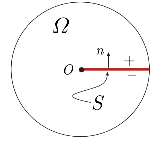
Figure 1: Schematic of setting for Volterra dislocation.

The region $\Omega$ in Fig. 1 denotes the unit disk in $\mathbb{R}^{2}$, whose centre $O$ is the origin of a Cartesian rectangular coordinate system. The region $\Omega$ is considered as the orthogonal cross-section of a right circular cylinder with symmetry axis in the $x_{3}$ direction. Let $S$ denote the intersection of $\Omega$ with the half-plane $x_{1}\geq 0$ within the $(x_{1},x_{3})$ plane; expressed otherwise, we have

$$S=\{(x_{1},x_{2})\in\Omega:x_{1}\geq 0,x_{2}=0\}.$$ (3.1)

Consider the Volterra dislocation problem of a static single straight dislocation along the $x_{3}-$axis under zero boundary tractions and no external body-force. On the slit region $\Omega\backslash S$ let the map $u:\Omega\backslash S\rightarrow\mathbb{R}^{3}$ represent the total displacement field that possesses the following limits as adjacent sides of $S$ are approached:

$$\begin{split}&u^{+}(x_{1}):=lim_{x_{2}\rightarrow 0^{+}}\,u(x_{1},x_{2}),\qquad x_{1}>0,\\ &u^{-}(x_{1}):=lim_{x_{2}\rightarrow 0^{-}}\,u(x_{1},x_{2}),\qquad x_{1}>0,\\ &(Grad\,u)^{+}(x_{1}):=lim_{x_{2}\rightarrow 0^{+}}\,Grad\,u(x_{1},x_{2}),\qquad x_{1}>0,\\ &(Grad\,u)^{-}(x_{1}):=lim_{x_{2}\rightarrow 0^{-}}\,Grad\,u(x_{1},x_{2}),\qquad x_{1}>0.\end{split}$$ (3.2)

We seek to determine the map $u$ that satisfies

$$Div\,C(Grad\,u)^{s}=0,\qquad x\in\Omega\backslash S,$$ (3.3)

subject to the conditions

$$\left[u\right]_{S} := u^{+}-u^{-}=b,\qquad x_{1}>0,$$ (3.4)

$$\left[C(Grad\,u)^{s}\right]_{S}.n := (C(Grad\,u^{+})^{s}-C(Grad\,u^{-})^{s}).n=0\ \ \mbox{for}\ \ x\neq 0,$$ (3.5)

$$C(Grad\,u)^{s}.N = 0\ \ \mbox{on}\ \partial\Omega.$$ (3.6)

Here, $b\in\mathbb{R}^{3}$ is a given constant Burgers vector, $\left[,\right]_{S}$ represents the jump across $S$, $N$ is the unit outward vector normal field on $\partial\Omega$ and $n=e_{2}$ is the unit vector normal on $S$.

Any such solution must satisfy $|Grad\,u(x_{1},x_{2})|\rightarrow\infty$ as $(x_{1},x_{2})\rightarrow(0,0)$, since the line integral of the displacement gradient taken anti-clockwise along any circular loop of arbitrarily small radius encircling the origin and starting from the “positive” side of $S$ and ending at the “negative” side must recover the finite value $-b$. This also implies that the displacement gradient field must diverge as $r^{-1}$ as $r\rightarrow 0$, where $r(x_{1},x_{2})$ is the distance of any point $(x_{1},x_{2})$ from the origin. Consequently, the linear elastic energy density is not integrable for bounded bodies that contain the origin.

With reference to Fig. 2, we now introduce the “slip region” given by

$$S_{l}=\left\{(x_{1},x_{2})\in\Omega\ |\ x_{1}\geq 0,\ |x_{2}|\leq\frac{l}{2}\right\},\ l>0.$$ (3.7)

and the “plasticity core”, a rectangular neighbourhood of the dislocation defined as

$$S^{l,c}=\left\{(x_{1},x_{2})\in\Omega\ |\ |x_{1}|<c,\ |x_{2}|\leq\frac{l}{2}\right\}.$$

The plasticity core in the limit $l\rightarrow 0$ represents the line segment

$$\left\{(x_{1},x_{2})\in\Omega\ |\ |x_{1}|<c,x_{2}=0\right\}.$$

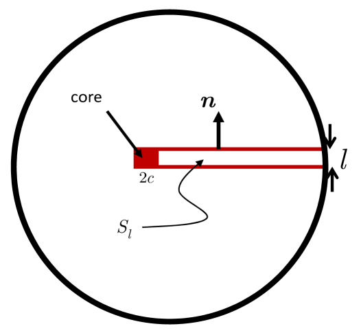
Figure 2: Schematic of setting for dislocation in plasticity theory.

The boundary value problem (3.2)-(3.6) for the Volterra dislocation is defined on $\Omega\backslash S$. In the plasticity theory of dislocations, however, the boundary value problem is defined on the whole of $\Omega$ and is specified by

$$\begin{split}&Div\,C(U^{(E)})^{s}=0,\qquad x\in\Omega,\\ &C\,(U^{(E)})^{s}.N=0,\qquad x\in\partial\Omega,\end{split}$$ (3.8)

where $U^{(E)}$, the elastic distortion tensor field, is smooth on $\Omega$.

The plastic distortion tensor field $U^{(P)}$ is defined as the difference between the gradient of the total displacement, denoted here to avoid confusion by $u^{d}:\Omega\rightarrow\mathbb{R}^{3}$, and the elastic distortion tensor $U^{(E)}$. Further physical motivation for these field variables will be presented in Sections 4 and 5. Accordingly, on noting that $u^{d}$ maps the whole of $\Omega$, we have

$$U^{(P)}(x)=Grad\,u^{d}(x)-U^{(E)}(x),\qquad x\in\Omega.$$ (3.9)

The explicit form selected for the plastic distortion tensor, taken as data, is given by

$$\begin{split}&U^{(P)}(x)=\begin{cases}&g(x_{1})\,\frac{1}{l}\,(b\otimes n)\ \ \mbox{in}\ \ S_{l},\\ &0\ \ \mbox{in}\ \ \Omega\backslash S_{l},\\ \end{cases}\\ \end{split}$$ (3.10)

where $b=(b_{1},b_{2},b_{3})$ is the constant Burgers vector, $n\in\mathbb{R}^{2}$ is the unit vector normal to the ‘layer’ $S_{l}$, $g(x_{1})=1$ for $x_{1}\geq c>0$, $g(x_{1})=0$ for $x_{1}\leq-c$, and $g$ is a monotone increasing function in $(-c,c)$. Hence, the non-uniformity of $g(x_{1})$ is confined to the plasticity core region $S^{l,c}$. We remark that $n=e_{2},\,b=b_{1}e_{1}+b_{2}e_{2}$ for an edge dislocation, while $n=e_{2},\,b=b_{3}e_{3}$ for a screw dislocation. The parameters $l$ and $c$ are significant in the physical modelling of dislocations: $l$ represents the interplanar spacing of a crystal and $c$ represents the non-vanishing core width of a crystal dislocation. Both $l$ and $c$ are observable quantities. From this point of view, the Volterra dislocation is an approximation (a large length-scale limit) of physical reality.

The component in the $x_{1}-$direction of each row of $U^{(p)}$ given by (3.10) is zero while their normal component along $n=e_{2}$ has a derivative in the $x_{1}-$direction that is non-zero only in the core region $S^{l,c}$. Therefore, $Curl\,U^{(P)}=:-\alpha$ is non-vanishing only in the core. (Jumps in $U^{(P)}$ in the normal direction across the layer $S_{l}$ are not sensed by the (distributional) $Curl$). It follows from Stokes’ Theorem that

$$\int_{Q}Curl\,U^{(P)}\,e_{3}\,dS=\int_{\partial Q}U^{(P)}.ds=b,$$ (3.11)

for any area patch $Q$ that completely covers the plasticity core, $S^{l,c}$, and whose closed bounding curve $\partial Q$ intersects the layer $S_{l}$ in points with $x_{1}$-coordinate greater than $c$. In the above, $e_{3}$ is the unit normal in the direction out of the plane in a right-handed sense.

Since the Volterra problem is posed on the region $\Omega\backslash S$, we seek to establish its equivalence with the plasticity problem on $\Omega\backslash S_{l}$ as $l\rightarrow 0$ and $c\rightarrow 0$.

The following orthogonal Stokes-Helmholtz decomposition holds for the field $U^{(P)}$:

$$U^{(P)}=Grad\,z-\chi,\qquad x\in\Omega,\\$$ (3.12)

where the second order tensor field $\chi$ satisfies

$$\begin{split}&Curl\,\chi=\alpha=-Curl\,U^{(P)},\qquad x\in\Omega,\\ &Div\,\chi=0,\qquad x\in\Omega,\\ &\chi.N=0\qquad x\in\partial\Omega.\end{split}$$ (3.13)

This structure has the important implication that $\chi$ is a continuous field on $\Omega$, for all values of $l\geq 0$ and $c>0$. When $c=0$, $\chi$ becomes a continuous field on the punctured domain $\Omega\backslash\{(0,0)\}$.

Let $\gamma(s)$ denote the line segment

$$\gamma(s)=(x_{1},0)+\left(-\frac{l}{2}+sl\right)n,\qquad s\in[0,1],\ \mathrm{for\ fixed\ }\ x_{1}>c.$$ (3.14)

By virtue of (3.11) and the continuity of $\chi$, the integral along $\gamma(s)$ of both sides of (3.12) yields

$$lim_{l\rightarrow 0}\int_{\gamma(s)}Grad\,z\,ds=\left[z\right]_{x_{1}>c}=z(x_{1},0^{+})_{x_{1}>c}-z(x_{1},0^{-})_{x_{1}>c}=lim_{l\rightarrow 0}\int_{\gamma(s)}U^{(P)}.ds=b\ .$$ (3.15)

The system (3.8) can be rewritten as

$$\begin{split}&u^{1}:=u^{d}-z,\qquad x\in\Omega,\\ &U^{(E)}=Grad\,u^{1}+\chi,\qquad x\in\Omega,\\ &Div\,C\left(Grad\,u^{1}\right)^{s}=-Div\,C\left(\chi\right)^{s},\qquad x\in\Omega,\\ &C\left(Grad\,u^{1}\right)^{s}.N=-C\ \left(\chi\right)^{s}.N,\qquad x\in\partial\Omega,\end{split}$$ (3.16)

and we note that for $c>0$, $u^{1}$ is a smooth field away from the core on $\Omega$ for all values of $l\geq 0$ (because $\chi$ is continuous and piecewise-smooth on $\Omega$). By integrating both sides of the expression $Grad\,u^{d}-Grad\,z=Grad\,u^{1}$ along the line segment $\gamma(s)$, taking the limit $l\rightarrow 0$, and appealing to (3.15), we obtain

$$\left[u^{d}\right]_{x_{1}>c}:=u^{d}(x_{1},0^{+})-u^{d}(x_{1},0^{-})=\left[z\right]_{x_{1}>c}=b.$$

The continuity of $\chi$ and the fact that $u^{1}$ is a solution to the system (3.16) for such a $\chi$ implies that for given $l\geq 0,\,c>0$, the total energy of the body is bounded; that is, $\frac{1}{2}\int_{\Omega}U^{(E)}:C\,U^{(E)}\,dx<\infty.$ Moreover, these properties also imply that for $c>0$ the tractions in the plasticity formulation are always continuous on any internal surface of $\Omega$. In particular, we have

$$\left[C\,\left(U^{(E)}\right)^{s}\right]_{x_{1}>c}n:=C\,\left(U^{(E)}\right)^{s}(x_{1},0^{+})n-C\,\left(U^{(E)}\right)^{s}(x_{1},0^{-})n=0,\ \ \mbox{for}\ \ c>0.$$

which is valid for points even in the plasticity core $S^{l,c}$.

Upon noting that $U^{(P)}=0$ in $\Omega\backslash S_{l}$ and also that $S_{l}\rightarrow S$ as $l\rightarrow 0$, we recover the following relations for $c>0$,

$$\begin{split}&Div\,C\,\left(Grad\,u^{d}\right)^{s}=0,\qquad x\in\Omega\backslash S,\\ &\left[u^{d}\right]_{x_{1}>c}=b,\\ &\left[C\,\left(Grad\,u^{d}\right)^{s}\right]_{x_{1}>c}n:=\left\{C\,\left(Grad\,u^{d}(x_{1},0^{+})\right)^{s}-C\left(Grad\,u^{d}(x_{1},0^{-}))^{s}\right)\right\}.n=0,\\ &C(Grad\,u^{d})^{s}.N=0,\qquad x\in\partial\Omega.\end{split}$$ (3.17)

The system (3.17) is formally identical to the “Volterra” system (3.2)-(3.6). It is in this sense that the plasticity solution is equivalent to the solution for the classical Volterra dislocation problem.

The plasticity solution is a very good approximation to the Volterra solution in $\Omega\backslash S_{l}$ even for small $l>0$ (compared to the radius of the body). Comparison of finite element approximations [ZAWB15] with the exact Volterra solution outside the plasticity core $S^{l,c}$ confirms that within $S_{l}$ and elsewhere the correspondence is excellent.

We have thus explained how a stationary solution to a Volterra dislocation problem may be regarded as the limiting form of solutions to a sequence of plasticity dislocation problems having particular plastic distortion tensors. We believe that the plasticity formulation is more general, practically versatile, and better able to deal with dislocations in elastic solids, especially those that are evolving. In the following sections we prove certain uniqueness results for the plasticity dislocation theory that directly apply to a body with an arbitrary collection of dislocation lines.

The discussion of the relationship between the Volterra and plasticity formulations has assumed that the plastic distortion is data. The treatment, however, in the next three sections adopts the dislocation density tensor, and not the plastic distortion tensor, as data and shows that the plastic distortion tensor is not always uniquely determined when this is the case.

4 Stationary (equilibrium) problem

The simply connected region $\Omega$, which we recall is occupied by a self-stressed linear inhomogeneous anisotropic compressible elastic material in equilibrium under zero applied body-force, prescribed dislocation density $\alpha$, and non-zero surface traction, is adopted as the reference configuration. The primary concern of this Section is to determine the self-stress occurring in $\Omega$, subject to relations (2.18)-(2.24), and to explore uniqueness issues. The appropriate traction boundary value problem is stated as

$$\alpha = Curl\,U^{(E)},\qquad x\in\Omega,$$ (4.1)

$$Div\,\sigma = Div\,C\left(U^{(E)}\right)^{s}=0,\qquad x\in\Omega,$$ (4.2)

$$\sigma.N = C\left(U^{(E)}\right)^{s}.N=g,\qquad x\in\partial\Omega,$$ (4.3)

where $g(x)$ is a prescribed statically admissible surface traction vector (i.e., the resultant of the surface force and moment arising from the traction distribution is zero).

4.1 Uniqueness of stress and elastic distortion

We prove for given dislocation density $\alpha$ and surface traction $g$ that the stress and the elastic distortion (up to a constant skew tensor) are unique.

Proposition 4.1.

In the traction boundary value problem (4.1)-(4.3) for specified elastic modulus tensor $C(x)$, the stress tensor is uniquely determined by the prescribed dislocation density $\alpha(x),\,x\in\Omega$ and surface traction $g(x),\,x\in\partial\Omega$. The elastic distortion tensor $U^{(E)}$ is unique up to a constant skew-symmetric tensor field on $\Omega$.

Proof. (Stated in [Wil67, Sec. 5] for infinite regions subject to asymptotically vanishing stress at large spatial distance.)

Kirchhoff’s uniqueness theorem [KP71] is not immediately applicable and we proceed as follows. Let $U^{(E)}_{1},\,U^{(E)}_{2}$ be solutions to (4.1)-(4.3) with $\widehat{U}^{(E)}:=U^{(E)}_{1}-U^{(E)}_{2}$. We have

$$\widehat{\sigma} := \sigma_{1}-\sigma_{2}$$ (4.4)

$$= C\left(\widehat{U}^{(E)}\right)^{s},\qquad x\in\Omega.$$

But $U^{(E)}_{1},\,U^{(E)}_{2}$ each satisfy relation (4.1) for prescribed dislocation density $\alpha$, and consequently

$$Curl\,\widehat{U}^{(E)}=0,\qquad x\in\Omega,$$ (4.5)

from which we infer the existence of a vector function $\widehat{z}$ such that $\widehat{U}^{(E)}=Grad\,\widehat{z},\,x\in\Omega$, since $\Omega$ is simply connected. It follows that $\widehat{\sigma}=C\left(Grad\,\widehat{z}\right)^{s}$ satisfies a zero-traction boundary condition, and uniqueness is implied by Kirchhoff’s theorem. Hence, the elastic distortion $U^{(E)}$ is unique to within a constant skew-symmetric tensor field on $\Omega.$

The solution to the traction boundary value problem (4.1)-(4.3) for spatially uniform elasticity and unbounded regions may be obtained using either Green’s function (see, for example, [Wil67, KGBB79]), or Fourier transform techniques (see, for example, [Sne51, Sne72, EFS56]), or stress functions as developed in [Krö58]. Of course, the most practically efficient method for solving the system (4.1)-(4.3) in full generality uses approximation techniques based on the finite element method described in e.g., [Jia98] (cf. [RA05]). Related convergence results and error estimates also are available. Kröner’s approach [Krö58] (with given dislocation density), even when applied to unbounded regions and homogeneous isotropic elasticity, shows that the stress and elastic strain(i.e., symmetric part of $U^{E}$) are unique but that the skew symmetric part of the elastic distortion remains undetermined. Unlike linear elasticity, the skew symmetric part of the elastic distortion in the present context of incompatible linear elasticity can be spatially inhomogeneous even if the symmetric part vanishes. Circumstances in which this may occur represent important physical configurations [RA05, BBSA14] e.g., stress-free dislocation walls.

Another method of solution for (4.1)-(4.3) follows [RA05] and writes $U^{(E)}$ as a gradient of a vector field plus a tensor field that in general is not curl-free. Both fields are then determined from equations (4.1)-(4.3). (The decomposition is not exactly that of Stokes-Helmholtz and is further discussed at the end of this section). The component potential functions of $U^{(E)}$ exist by explicit construction using standard methods in potential theory and elasticity theory.We seek a solution of the form

$$U^{(E)}=-Grad\,z^{(E)}+\chi^{(E)},\qquad x\in\Omega,$$ (4.6)

where the function $\chi^{(E)}$ satisfies

$$Curl\,\chi^{(E)} = \alpha,\qquad x\in\Omega,$$ (4.7)

$$Div\,\chi^{(E)} = 0,\qquad x\in\Omega,$$ (4.8)

$$\chi^{(E)}.N = 0,\qquad x\in\partial\Omega.$$ (4.9)

The vector function $z^{(E)}$ in (4.6) is then chosen to satisfy the system obtained on elimination of $U^{(E)}$ between (4.6) and (4.2) and (4.3). We have

$$Div\,C\left(Grad\,z^{(E)}\right)^{s} = Div\,C\left(\chi^{(E)}\right)^{s},\qquad x\in\Omega,$$ (4.10)

$$\left(C\left(Grad\,z^{(E)}\right)^{s}\right).N = -g+\left(C\left(\chi^{(E)}\right)^{s}\right).N,\qquad x\in\partial\Omega.$$ (4.11)

Note that the tensor function $\chi^{(E)}$ is uniquely determined by (4.7)-(4.9) for prescribed $\alpha(x)$: for, let $\chi^{(E)}_{1},\,\chi^{(E)}_{2}$ be solutions. Define $\chi^{(E)}(x)=\chi^{(E)}_{1}(x)-\chi^{(E)}_{2}(x)$ so that $Curl\,\chi^{(E)}(x)=0,\,x\in\Omega$. Therefore, $\chi^{(E)}(x)=Grad\,\phi^{(E)}(x)$ for some twice continuously differentiable vector function $\phi^{(E)}(x)$ as $\Omega$ is simply connected. On substitution in (4.8) and (4.9), we conclude that $\phi^{(E)}$ satisfies the harmonic Neumann boundary value problem

$$Div\,Grad\,\phi^{(E)} = 0,\qquad x\in\Omega,$$

$$Grad\,\phi^{(E)}.N = 0,\qquad x\in\partial\Omega.$$

Consequently, $\phi^{(E)}$ is constant and therefore $\chi^{(E)}=0$.

Upon substitution of the uniquely determined $\chi^{(E)}$ in (4.10) and (4.11), we obtain a linear elastic traction boundary value problem for $z^{(E)}$ under non-zero body-force and surface traction. It can be verified that the required necessary conditions are satisfied for the vanishing of the sum of forces and moments due to the boundary load $g$ and conditions on $\chi^{(E)}$. Uniqueness theorems in linear elastostatics state that $z^{(E)}(x)$ is unique to within an infinitesimal rigid body displacement. Hence, a solution $U^{(E)}$ to (4.1)-(4.3) exists and is unique (up to a constant skew-symmetric tensor) by Proposition 4.1.

Conversely, suppose that $U^{(E)}$ is a given solution of (4.1)-(4.3). Then a unique Stokes-Helmholtz decomposition of $U^{(E)}$ exists given by

$$U^{(E)}=-Grad\,z+\chi,\qquad x\in\Omega,$$ (4.12)

where $z,\,\chi$ respectively are sufficiently smooth vector and tensor functions that satisfy

$$Curl\,\chi = \alpha,\qquad x\in\Omega,$$ (4.13)

$$Div\,\chi = 0,\qquad x\in\Omega,$$ (4.14)

$$\chi.N = 0,\qquad x\in\partial\Omega,$$ (4.15)

$$Div\,Grad\,z = -Div\,U^{(E)},\qquad x\in\Omega,$$ (4.16)

$$Grad\,z.N = -U^{(E)}.N,\qquad x\in\partial\Omega.$$ (4.17)

Although the component potentials $\chi,\chi^{(E)},z,z^{(E)}$ apparently satisfy different sets of governing equations, nevertheless, it is easily seen that the functions $z^{(E)}$ and $\chi^{(E)}$ satisfy the relations

$$\begin{split}&\chi=\chi^{(E)},\ \ \ Grad\,z=Grad\,z^{(E)},\\ &z=z^{(E)}\ \ \mbox{up to a translation.}\end{split}$$

Notice that as $U^{(E)}$ is uniquely determined in this stationary problem to within a skew-symmetric tensor, neither the fields $Div\,U^{(E)}$ on the domain $\Omega$ nor $U^{(E)}.N$ on the boundary $\partial\Omega$ can be arbitrarily prescribed.

Remark 4.1 (Reduction to classical linear elasticity of the stationary problem).

We seek necessary and sufficient conditions for classical linear elasticity to be recovered from (4.1)-(4.3). A classical linear elastic solution in this context corresponds to (4.2)-(4.3) in which $Curl\,U^{(E)}=0$. It is straightforward to see that $\alpha=0$ is the necessary and sufficient condition for $U^{(E)}$ satisfying (4.1)-(4.3) to be a classical linear elastic solution.

Remark 4.2 (Conditions in terms of the decomposition (4.12)).

Necessary and sufficient conditions for $U^{(E)}$ satisfying (4.1)-(4.3) to be a classical linear elastic solution may be expressed in terms of the potential functions occurring in (4.12). When $Curl\,U^{(E)}=\alpha=0$ in (4.1)-(4.3), (4.13)-(4.15) necessarily give $\chi=0$. Also, the potential $z$ then satisfies $Div(C\,Gradz)^{s}=0$ on $\Omega$ and $(C(Gradz)^{s}).N=-g$ on $\partial\Omega$. Conversely, if $\chi=0$ and the potential $z$ satisfies the conditions in the previous sentence, then $U^{(E)}$ defined by (4.12) is a classical linear elastic solution in this context, i.e., $Curl\,U^{(E)}=0$ and (4.2)-(4.3) are satisfied.

4.2 Example: Stationary screw dislocation in the whole space

The technique based on the Stokes-Helmholtz decomposition applied to the stationary problem in Section 4.1 is illustrated by a simple example. Consider the whole space occupied by a homogeneous isotropic compressible linear elastic material that contains a single stationary straight line screw dislocation located at the origin and directed along the positive $x_{3}$-axis. For simplicity, no applied body-force acts, and appropriate fields, including the Stokes-Helmholtz potential $z^{(E)}$, asymptotically vanish to suitable order. In particular, the traction $g(x)$ prescribed in (4.3) vanishes in the limit as $x_{i}x_{i}\rightarrow\infty.$

The dislocation density is specified to be

$$\alpha(x)=|b|\delta(x_{1})\delta(x_{2})e_{3}\otimes e_{3},\qquad x\in\mathrm{I\!R\!}^{3},$$ (4.18)

where we recall that $\delta(.)$ represents the Dirac delta distribution, and $e_{i},\,i=1,2,3,$ are the unit coordinate vectors. The multiplicative constant $|b|$ is selected to ensure that $|b|$ is the magnitude of the corresponding Burgers vector. Without loss, all dependent field variables are assumed independent of $x_{3}$ and to be of sufficient smoothness.

Consider the decomposition (4.6) for the elastic distortion tensor $U^{(E)}$. In view of relation (2.33), a tensor function $A^{(E)}$ exists that satisfies

$$\chi^{(E)}=-Curl\,A^{(E)},\qquad Div\,A^{(E)}=0,\qquad x\in\mathrm{I\!R\!}^{2}.$$ (4.19)

and

$$\Delta\,A^{(E)}(x)=\alpha(x),\qquad x\in\mathrm{I\!R\!}^{2}.$$

Substitution from (4.18) leads to

$$\Delta\,A^{(E)}_{33}(x)=\alpha_{33}=|b|\delta(x_{1})\delta(x_{2}),\qquad x\in\mathrm{I\!R\!}^{2}.$$ (4.20)

All other components of $A^{(E)}$ are harmonic in $\mathrm{I\!R\!}^{3}$ and are supposed to vanish asymptotically at large spatial distance. Therefore, they vanish identically by Liouville’s Theorem. The distributional solution to (4.20) is given by

$$A^{(E)}_{33}=\frac{|b|}{2\pi}\ln R,\qquad R^{2}=x_{\beta}x_{\beta},$$ (4.21)

and in consequence from (4.19) the non-zero components of $\chi^{(E)}$ are

$$\chi^{(E)}_{31}(x_{1},x_{2}) = -\frac{|b|}{2\pi}\frac{x_{2}}{R^{2}},$$ (4.22)

$$\chi^{(e)}_{32}(x_{1},x_{2}) = \frac{|b|}{2\pi}\frac{x_{1}}{R^{2}},$$ (4.23)

which show that

$$\left(Div\,\chi^{(E)}\right)_{\beta} = 0,$$

$$\left(Div\,\chi^{(E)}\right)_{3} = \chi_{31,1}+\chi_{32,2}$$ (4.24)

$$= \frac{|b|}{2\pi}\left[-\frac{2x_{1}x_{2}}{R^{4}}+\frac{2x_{2}x_{1}}{R^{4}}\right]$$

$$= 0,$$ (4.25)

and (4.8) is satisfied in the sense of distributions. It can also be verified that the solution (4.21) satisfies $Div\,A^{(E)}=0$, so that $\chi^{(E)}:=-Curl\,A^{(E)}$ implies $Curl\,\chi^{(E)}=\alpha$ from (4.20).

The vector function $z^{(E)}(x_{1},x_{2})$ satisfies (4.10), the right side of which by virtue of (4.8), (4.22), and (4.23) becomes

$$\left[C\chi^{(E)}(x_{1},x_{2})\right]_{,j} = \left[\lambda\chi^{(E)}_{kk}\delta_{ij}+\mu\left(\chi^{(E)}_{ij}+\chi^{(E)}_{ji}\right)\right]_{,j}$$

$$= \mu\left(\chi^{(E)}_{ij,j}+\chi^{(E)}_{ji,j}\right)$$

$$= 0,$$

where $\lambda$ and $\mu$ are the Lamé constants, and $\delta_{ij}$ is the Kronecker delta.

Consequently, $z^{(E)}(x_{1},x_{2})$ is the solution to the equilibrium equations of linear elasticity on the whole space. Assume that $z^{(E)}(x_{1},x_{2})$ is bounded as $R\rightarrow\infty$. Liouville’s Theorem implies that $z^{(E)}(x_{1},x_{2})$ is constant. Accordingly, by (4.6) the non-zero components of the asymmetric elastic distortion tensor are

$$U^{(E)}_{31}(x_{1},x_{2}) = -\frac{|b|x_{2}}{2\pi R^{2}},$$ (4.26)

$$U^{(E)}_{32}(x_{1},x_{2}) = \frac{|b|x_{1}}{2\pi R^{2}}.$$ (4.27)

Let $\partial\Sigma$ be the circle of radius $a$ whose centre is at the origin. The Burgers vector corresponding to the elastic distortion tensor whose non-zero components are (4.26) and (4.27) may be calculated from (2.19) and gives $b=(0,0,b_{3})$ where

$$b_{3}=\oint_{\partial\Omega}U^{E)}_{3\beta}dx_{\beta}=|b|,$$

as previously stated.

Well-known expressions (see,for example, [HL82]) are easily derived for the unique non-zero stress components, namely

$$\sigma_{31}(x_{1},x_{2}) = -\frac{\mu|b|x_{2}}{2\pi R^{2}},$$ (4.28)

$$\sigma_{32}(x_{1},x_{2}) = \frac{\mu|b|x_{1}}{2\pi R^{2}}.$$ (4.29)

5 The quasi-static boundary value problem

It is supposed that the dislocation density evolves as a prescribed tensor function of both space and time. The precise mode of evolution is unimportant for immediate purposes since the dislocation density is adopted as data. The body is subject to specified applied time-dependent surface boundary conditions on tractions and/or total displacements (see (5.1)), although the applied body-force is assumed to vanish (for simplicity and without loss of generality). The time-varying data causes the stress $\sigma(x,t)$ and elastic distortion $U^{(E)}(x,t)$ also to be time- dependent, and the body to change shape with time. Prediction of the elastic distortion, stress, and change of shape necessitates introduction of the total displacement field $u(x,t)$, that is identical to the field $u^{d}$ of Sec. 3, but which we henceforth refer to simply as $u$ for notational simplicity. The corresponding state-space consists of pairs $\left(u,U^{(E)}\right)$. We consider a re-parametrization of the state space, and for this purpose recall that (2.25), namely

$$U^{(P)}:=Grad\,u-U^{(E)},\qquad(x,t)\in\Omega\times[0,T),$$ (5.1)

is employed to define the plastic distortion tensor. The set of pairs $\left(u,U^{(P)}\right)$ then forms a new state-space. Section 3 discusses the connection between (5.1) and the classical Volterra mathematical model of dislocations.

Relation (2.21) between the dislocation density and elastic distortion remains valid for time evolution problems, and in conjunction with (5.1) leads to the formulae

$$\alpha = Curl\,U^{(E)}$$ (5.2)

$$= Curl\,\left(Grad\,u-U^{(P)}\right)$$

$$= -Curl\,U^{(P)},\qquad(x,t)\in\Omega\times[0,T),$$

where $[0,T),\,T>0,$ is contained in the maximal interval of existence.

The constitutive relation (2.23) also remains valid and expressed in terms of the plastic distortion becomes

$$\sigma = C\left(U^{(E)}\right)^{s}$$ (5.3)

$$= C\left(Grad\,u-U^{(P)}\right)^{s},\qquad(x,t)\in\Omega\times[0,T).$$

The inertial term $\rho\ddot{u}$ is discarded in the quasi-static approximation to the initial boundary value problem. The time-dependence, however, of all other field variables is retained with time serving as a parameter. The quasi-static boundary value problem, including (5.2) repeated here for completeness, at each $t\in[0,T)$, therefore becomes

$$\alpha=-Curl\,U^{(P)},\qquad(x,t)\in\Omega\times[0,T),$$ (5.4)

and

$$Div\,\sigma=0,\qquad(x,t)\in\Omega\times[0,T),$$ (5.5)

or

$$Div\,C\left(Grad\,u-U^{(P)}\right)^{s}=0,\qquad(x,t)\in\Omega\times[0,T),$$ (5.6)

subject to either traction boundary conditions

$$\sigma.N = g,\qquad(x,t)\in\partial\Omega\times[0,T),$$ (5.7)

or mixed boundary conditions

$$u=h,\qquad(x,t)\in\partial\Omega_{1}\times[0,T),$$ (5.8)

$$\sigma.N=g,\qquad(x,t)\in\partial\Omega_{2}\times[0,T),$$ (5.9)

where $\partial\Omega=\partial\Omega_{1}\cup\partial\Omega_{2}$, $\partial\Omega_{1}\cap\partial\Omega_{2}=\emptyset$. The vector functions $h(x,t)$ and $g(x,t)$ are prescribed.

The traction boundary value problem, specified by (5.4), (5.6) and (5.7), is formally identical to the stationary traction boundary value problem studied in Section 4. We conclude that the quasi-static stress tensor is uniquely determined while the elastic distortion tensor is unique to within a skew-symmetric tensor. Without modification, however, the previous argument cannot be applied to prove uniqueness of either the plastic distortion tensor or the total displacement.

To investigate this aspect, for each $t\in[0,T)$ let the plastic distortion be completely represented by its Stokes-Helmholtz decomposition in the form

$$U^{(P)}=Grad\,z-\chi,\qquad(x,t)\in\Omega\times[0,T),$$ (5.10)

where the incompatible smooth tensor potential $\chi$ satisfies the system

$$\alpha = Curl\,\chi,\qquad(x,t)\in\Omega\times[0,T),$$ (5.11)

$$Div\,\chi = 0,\qquad(x,t)\in\Omega\times[0,T),$$ (5.12)

$$\chi.N = 0,\qquad(x,t)\in\partial\Omega\times[0,T).$$ (5.13)

Similar comments contained in Section 4.1 regarding uniqueness of the tensor $\chi^{(E)}(x)$ and its vanishing with $\alpha(x)$ apply to the tensor $\chi(x,t)$ and the time-dependent dislocation density $\alpha(x,t)$.

Define the vector functions $\widetilde{r}(x,t),\,\widetilde{s}(x,t)$ by

$$\widetilde{r} = Div\,U^{(P)},\qquad(x,t)\in\Omega\times[0,T),$$ (5.14)

$$\widetilde{s} = U^{(P)}(x,t).N,\qquad(x,t)\in\partial\Omega\times[0,T).$$ (5.15)

In terms of the continuously differentiable vector function $z(x,t)$ appearing in (5.10) for each $t\in[0,T)$, these definitions are equivalently expressed as

$$Div\,Grad\,z = \widetilde{r},\qquad(x,t)\in\Omega\times[0,T),$$ (5.16)

$$Grad\,z.N = \widetilde{s},\qquad(x,t)\in\partial\Omega\times[0,T).$$ (5.17)

The vector -valued functions $\widetilde{r}(x,t),\,\widetilde{s}(x,t)$ at each time instant are restricted by the compatibility condition

$$\int_{\Omega}\widetilde{r}\,dx=\int_{\partial\Omega}\widetilde{s}\,dS,$$ (5.18)

but otherwise may be arbitrarily selected. Here, we consider them as data, along with the dislocation density tensor.

Remark 5.1.

In the full stress-coupled theory of dislocation mechanics as a non-standard model within the structure of classical plasticity theory[Mur63a, Kos79, AZ15, ZAWB15], physically well-motivated and, in principle, experimentally observable evolution equations for the dislocation density and the plastic distortion arise naturally. There is of course some redundancy between the specification of both ingredients, and in the above models this is achieved in a self-consistent manner. On the other hand, as already demonstrated, the stationary traction boundary value problem of dislocation mechanics ((4.1)- (4.3)) is well-posed simply through the specification of the dislocation density. It is then reasonable to ask what extra minimal ingredients beyond the specification of the dislocation density are required to have a well-posed model of plasticity arising from the evolution of dislocations. This question is among our primary concerns, without regard to the ease with which these minimal, extra ingredients can be physically determined.

For specified $\widetilde{r}(x,t),\,\widetilde{s}(x,t)$, the solution to the Neumann boundary value problem (5.16) and (5.17) is unique to within an arbitrary vector function of time $\widetilde{d}(t)$, and may be obtained by any standard method in potential theory.

The results derived so far in this Section are summarised in the next Proposition.

Proposition 5.1.

Consider the plastic distortion tensors $U^{(P)(1)}(x,t),\,U^{(P)(2)}(x,t)$ that correspond to the same dislocation density $\alpha(x,t)$, and possess the same divergence and surface normal components. On appealing to the respective Stokes-Helmholtz decompositions, our previous results show that $U^{(P)(1)}=U^{(P)(2)}$. Consequently, specification of $\alpha,\,\widetilde{r},\,\widetilde{s}$ uniquely determines the plastic distortion.

We examine the implications of supposing that $\widetilde{r},\widetilde{s}$ are arbitrarily assigned but still subject to a prescribed dislocation density. In the same manner as previously shown, the dislocation density uniquely determines the tensor $\chi$ in the Stokes-Helmholtz decomposition (5.10), but arbitrary prescription of the vector functions $\widetilde{r}(x,t),\,\widetilde{s}(x,t)$ means that $Grad\,z(x,t)$ remains indeterminate. Thus,

Remark 5.2.

The quasi-static problem of moving dislocation fields with non-zero dislocation density data admits an inevitable fundamental structural ambiguity pivotal to the discussion of uniqueness.

The ambiguity is further explored in Section 6 devoted to moving dislocations subject to material inertia.

We describe a slightly different proof to that in Proposition 4.1 to establish uniqueness of the stress and elastic distortion in the quasi-static traction boundary value problem. Substitution of (5.10) in (5.6) and (5.7) yields

$$Div\,C\left(Grad\,(u-z)+\chi\right)^{s}=0,\qquad(x,t)\in\Omega\times[0,T),\\$$ (5.19)

$$C\left(Grad\,(u-z)\right)^{s}.N=g-\left(C\left(\chi\right)^{s}\right).N,\qquad x\in\partial\Omega\times[0,T).$$ (5.20)

The tensor function $\chi$ appearing in these expressions is uniquely determined by the dislocation density $\alpha$. In consequence, the Kirchhoff uniqueness theorem of linear elastostatics ensures that $(u-z)$ is uniquely determined by the system (5.19) and (5.20) to within an arbitrary rigid body displacement irrespective of the choice of $\widetilde{r},\,\widetilde{s}$. This enables us to further conclude that (5.1), rewritten as

$$U^{(E)}=Grad\,\left(u-z\right)+\chi,\qquad(x,t)\in\Omega\times[0,T),$$

implies the uniqueness of the elastic distortion (up to a constant skew-symmetric tensor field). Furthermore, the stress, given by

$$\sigma=C\left(Grad\,\left(u-z\right)+\chi\right)^{s},\qquad(x,t)\in\Omega\times[0,T),$$

is unique.

The vector functions $\widetilde{r},\,\widetilde{s}$ uniquely determine $z$ to within an arbitrary vector function of time only. Since it has just been shown that $(u-z)$ is unique to within an arbitrary rigid body displacement, the total displacement $u$ is also unique to within an arbitrary rigid body displacement dependent on time as a parameter. Uniqueness is lost once $\widetilde{r},\,\widetilde{s}$ are arbitrarily chosen.

In the mixed boundary value problem, and also the displacement boundary value problem for which $\partial\Omega_{2}=\emptyset$, prescription of the boundary term $h$ requires that $u$ and $z$ are separately considered. The system (5.11)-(5.13) still enables $\alpha$ to uniquely determine $\chi$. However, although $z(x,t)$ is uniquely determined to within an arbitrary vector $d(t)$ from (5.16) and (5.17), it still inherits the arbitrariness of $\widetilde{r},\,\widetilde{s}$. Nevertheless, specification of $\,\widetilde{r},\,\widetilde{s}\,$ leads to a unique $Grad\,z$ which upon insertion into the system (5.6), (5.8), (5.9) enables $u$ to be uniquely determined. Then $U^{(E)}(x,t)$ can be calculated from (5.1) and the stress from (5.3). However, like $z$, the field variables $U^{(P)}(x,t),\,u(x,t),\,U^{(E)}(x,t),\,\sigma(x,t)$ are ambiguous once $\widetilde{r},\,\widetilde{s}$ become arbitrary.

It is of interest to characterize the dependence of the fields $U^{(E)}$ and $\sigma$ on $\widetilde{r},\,\widetilde{s}$ by rewriting (5.6), (5.8), (5.9 as

$$Div\,C\left[(Grad\,(u-z))^{s}\right] = -Div\,C\left(\chi\right)^{s},\qquad(x,t)\in\Omega\times[0,T),$$

$$(u-z) = (h-z),\qquad(x,t)\in\partial\Omega_{1}\times[0,T),$$

$$C\left[(Grad\,(u-z))^{s}\right].N = g(x,t)-C\left(\chi\right)^{s}.N,\qquad(x,t)\in\partial\Omega_{2}\times[0,T),$$

where $z$ is obtained from (5.16) and (5.17) in terms of $\widetilde{r},\,\widetilde{s}$. It now follows that $(u-z)$, and consequently $Grad\,(u-z)$, $U^{(E)},$ and the stress $\sigma$, depend on $\widetilde{r},\,\widetilde{s}$ only through the values of $z$ on the boundary $\partial\Omega_{1}$. The arbitrariness of $z$ up to a vector function of time has no effect on the determination of either $U^{(E)}$ or $\sigma$. In particular, the stress depends on $z$ through the term $Grad\,\left(u-z\right)^{s}$.

These conclusions are assembled in the following Table, where the qualification to within appropriate rigid body displacements is understood.

Specified dislocation density: Uniqueness in BVP’s
	Traction BVP	Mixed BVP	All BVP: $\widetilde{r},\,\widetilde{s}$ specified
$u$	No	No	Yes
$U^{(P)}$	No	No	Yes
$U^{(E)}$	Yes	No	Yes
$\sigma$	Yes	No	Yes

Remark 5.3 (Reduction to classical linear elasticity of quasi-static boundary value problem).

We seek necessary and sufficient conditions for quasi-static classical linear elasticity to be recovered from (5.4)-(5.9). We define a pair of fields $(u,U^{(E)})$, or equivalently $(u,U^{(P)})$, satisfying (5.4)-(5.9) as a classical linear elastic solution with stress given by $C\,(Grad\,u)^{s}$ provided $Curl\,U^{(E)}=0$ (or equivalently $Curl\,U^{(P)}=0$) and the total displacement $u$ satisfies the equations obtained from (5.6)-(5.9) on formally setting $U^{(P)}=0$.

It is then easy to see that necessary and sufficient conditions for a solution $(u,U^{(P)}$) of (5.6),(5.8), and(5.9) to be a classical linear elastic solution with stress given by $C\,(Grad\,u)^{s}$ are that

$$\begin{split}Div\,C\left(U^{(P)}\right)^{s}&=0,\qquad x\in\Omega,\\ \left(C\left(U^{(P)}\right)^{s}\right).N&=0,\qquad x\in\partial\Omega_{2},\\ Curl\,U^{(P)}&=0\qquad x\in\Omega.\end{split}$$ (5.21)

The argument may be conducted in terms of the Stokes-Helmholtz decomposition (5.10). Since $Curl\,U^{(P)}=0$ is equivalent to $\chi=0$ on $\Omega$, it follows that (5.21) becomes

$$\begin{split}Div\,C\left(Grad\,z)^{s}\right)&=0,\qquad x\in\Omega,\\ \left(C\,(Grad\,z)^{s}\right).N&=0,\qquad x\in\partial\Omega_{2},\\ \chi&=0\qquad x\in\Omega.\end{split}$$ (5.22)

Consequently, (5.22) are the necessary and sufficient conditions for a classical linear elastic solution to be given by a triple $(u,\,\chi,\,z)$ that satisfies (5.4)-(5.9) and defines a pair $(u,\,U^{(P)})$ through (5.10).

6 Nonuniqueness for moving dislocations with material inertia

We continue the discussion of a time evolving continuous dislocation distribution of specified density $\alpha(x,t)$, but now retain inertia. For moving dislocations, the relation (2.21) and constitutive relations (2.23) together with (5.1) continue to hold. The quasi-static equilibrium equation (5.5), however, is replaced by the equation of motion (2.27), which for convenience is repeated :

$$Div\,\sigma=\rho\ddot{u},\qquad(x,t)\in\Omega\times[0,T),$$ (6.1)

where $\rho(x)>0$ is the positive mass density of the elastic body.

In terms of the total displacement vector $u(x,t)$, for which initial Cauchy data is required, and plastic distortion tensor $U^{(P)}(x,t)$, the initial boundary value problem studied in this Section is given by

$$\alpha=-Curl\,U^{(P)},\qquad(x,t)\in\Omega\times[0,T),$$ (6.2)

$$\sigma=C\left(Grad\,u-U^{(P)}\right)^{s},\qquad(x,t)\in\Omega\times[0,T),$$ (6.3)

$$Div\,C\left(Grad\,u-U^{(P)}\right)^{s}=\rho\ddot{u},\qquad(x,t)\in\Omega\times[0,T),$$ (6.4)

with displacement boundary conditions

$$u=h,\qquad(x,t)\in\partial\Omega_{1}\times(0,T),$$ (6.5)

traction boundary conditions

$$C\left(Grad\,u-U^{(P)}\right)^{s}.N=g,\qquad(x,t)\in\partial\Omega_{2}\times[0,T),$$ (6.6)

and initial conditions

$$u(x,0)=l(x),\qquad\dot{u}(x,0)=f(x),\qquad x\in\Omega,$$ (6.7)

where $\partial\Omega=\partial\Omega_{1}\cup\partial\Omega_{2}$, , $\partial\Omega_{1}\cap\partial\Omega_{2}=\emptyset$, $\partial\Omega_{2}(t=0)=\partial\Omega$ and $h(x,t),\,g(x,t),\,l(x),\,f(x)$ are prescribed functions.

Remark 6.1.

When dealing with plasticity and dislocations, there is no natural reference configuration that can be chosen. The as-received configuration of the body may well be plastically deformed with respect to some prior reference and support a non-vanishing stress field. Moreover, it is not physically reasonable to require that some prior distinguished reference be known to determine the future evolution of the body and its state from the as-received one. Thus, the initial condition on the displacement is most naturally specified as $l=0,x\in\Omega$ in (6.7). However, for many problems a displacement from a prior reference may be unambiguously known at $t=0$, e.g., when interrogating a motion of some reference from an intermediate state after some time has elapsed and considering the motion from this ‘intermediate’ state now as the reference. It is for such situations that we allow for a general non-vanishing initial condition on displacement as in (6.7).

Of note is also the fact that the formulation involves no displacement boundary condition at $t=0$, allowing only the specification of tractions on the entire boundary at the initial time. These issues are further dealt with in Step 2 of the proof of Theorem 6.1.

Unique specification of $U^{(P)}(x,t)$ implies that $u(x,t)$ is the solution to an initial mixed boundary value problem in linear elasticity subject to known body-force in (6.4), known boundary conditions (6.5) and (6.6), and known initial conditions (6.7). Uniqueness of $u$ then follows from appropriate theorems in linear elastodynamics (see [KP71]) and implies the unique determination of the elastic distortion $U^{(E)}(x,t)$ and stress $\sigma(x,t)$. However, the plastic distortion $U^{(P)}(x,t)$ is not uniquely determined from (6.2) for given dislocation density $\alpha(x,t)$. Indeed, we have the following Theorem.

Theorem 6.1 (Non-uniqueness).

The stress tensor $\sigma,$ elastic distortion tensor $U^{(E)}$, total displacement vector $u,$ and plastic distortion tensor $U^{(P)}$, belonging to the linear system (6.2)-(6.7) are not in general uniquely determined by the prescribed data $\alpha,\,h,\,g,\,l,\,\mbox{and }f$. Exceptions are noted below.

Proof

The proof proceeds in three main steps and involves the Stokes-Helmholtz decomposition.

Step 1. Stokes-Helmholtz decomposition.

Consider the relation (6.2). The Stokes-Helmholtz decomposition completely represents $U^{(P)}$ as

$$U^{(P)}(x,t)=Grad\,z(x,t)-\chi(x,t),\qquad(x,t)\in\Omega\times[0,T),$$ (6.8)

where the incompatible smooth tensor potential function $\chi(x,t)$ satisfies the system (5.11)-(5.13). The dislocation density $\alpha(x,t)$ therefore uniquely determines $\chi(x,t)$ for each $t\in[0,T)$. We recall that the boundary condition (5.13) entails no loss and in particular ensures that $\chi$ vanishes with $\alpha.$

The boundary value problem (5.16)-(5.18) for the vector potential function $z(x,t)$ is replaced by the analogous system for the time derivative $\dot{z}(x,t)$ which accordingly for each $t\in[0,T)$ satisfies

$$Div\,Grad\,\dot{z} = r,\qquad(x,t)\in\Omega\times[0,T),$$ (6.9)

$$Grad\,\dot{z}.N = s,\qquad(x,t)\in\partial\Omega\times[0,T),$$ (6.10)

for vector functions $r(x.t),\,s(x,t)$ constrained at each time instant to satisfy the compatibility condition

$$\int_{\Omega}r\,dx=\int_{\partial\Omega}s\,dS,\qquad t\in[0,T).$$ (6.11)

As remarked in Section 5, prescription of only the dislocation density $\alpha(x,t)$, but with the vector functions $r(x,t),\,s(x,t)$ arbitrarily ascribed, creates structural ambiguities which are considered in Steps $2$ and $3$. Our aim is to identify the essential role of the fields $r,s$ in the determination of uniqueness.

When $r(x,t)$ and $s(x,t)$ are prescribed, the solution $\dot{z}(x,t)$ to the Neumann system (6.9)-(6.11) is unique to within an arbitrary function of time, $d(t)$ for $t\in[0,T)$. Let $z^{(0)}(x)$ denote the initial value of $z(x,t)$. A time integration of the solution $\dot{z}(x,t)$ then shows that $z(x,t)-z^{(0)}(x)$ is unique to within an arbitrary vector function of time, say $d_{1}(t)$. However, the unique determination of stress and total displacement in the problem (6.2)-(6.7) depends on the uniqueness of $U^{(P)}$, which in turn depends upon that of $Grad\,z(x,t)$. Thus, the arbitrary vector function $d_{1}(t)$ is immaterial and can be ignored.

The next step is to calculate the initial terms $Grad\,z^{(0)}(x)$ and $U^{(P)}(x,0)$.

Step 2. Initial physical data for $Grad\,z$ and $U^{(P)}$. It is a natural requirement in dislocation and plasticity theories that assigned initial data should be observable in the current configuration and without the requirement of the knowledge a distinguished prior reference.

The evolution of $U^{(P)}$ depends on its initial value in the as-received configuration of the body. Thus, it is important to ascertain whether or not initial values of $U^{(P)}$ can be derived from measurements conducted on the body in the initial configuration. In this respect, we suppose that the dislocation density $\alpha(x,t)$ is a physically measurable observable for all $(x,t)\in\Omega\times[0,T)$ whose initial value $\alpha^{(0)}(x)$ is therefore assumed known.

We additionally suppose that initial displacement, velocities, and accelerations can be physically measured so that we have

$$\lim_{t\rightarrow 0}{\alpha(x,t)} = \alpha^{(0)}(x),\qquad x\in\Omega,$$ (6.12)

$$u(x,0) = l(x),\quad\dot{u}(x,0)=f(x),\quad\ddot{u}(x,0)=m(x),\qquad x\in\Omega,$$ (6.13)

where $\alpha^{(0)}(x),\,l(x),\,f(x),\,m(x)$ are known from practical observation. As already mentioned, $l=0,x\in\Omega$ is expected to be a specification that is commonplace.

The initial value $U^{(P)(0)}(x)$ of $U^{(P)}(x,t)$ is completely represented by the corresponding Stokes-Helmholtz decomposition given by

$$U^{(P)(0)}=Grad\,z^{(0)}-\chi^{(0)},\qquad x\in\Omega.$$ (6.14)

By continuity, the equations of motion (6.4) and boundary conditions (6.5) and (6.6) are taken to hold in the limit as $t\rightarrow 0^{+}$.

In accordance with the previous treatment, the initial value $\chi^{(0)}(x)$ is uniquely determined from the system

$$Curl\,\chi^{(0)} = \alpha^{(0)},\qquad x\in\Omega,$$ (6.15)

$$Div\,\chi^{(0)} = 0,\qquad x\in\Omega,$$ (6.16)

$$\chi^{(0)}.N = 0,\qquad x\in\partial\Omega,$$ (6.17)

Substitution of (6.7) and (6.12)-(6.14) in the equations of motion (6.4), assumed valid at $t=0$, leads to the equation for the initial value $z^{(0)}(x)$ of $z(x,t)$. We obtain

$$Div\,C\left(Grad\,\left(l-z^{(0)}\right)\right)^{s}+Div\,C\left(\chi^{(0)}\right)^{s}=\rho m,\qquad x\in\Omega,$$ (6.18)

which after rearrangement becomes

$$Div\,C\left(Grad\,z^{(0)}\right)^{s}-\rho F=0,\qquad x\in\Omega,$$ (6.19)

where the pseudo-body force $F(x)$ is uniquely defined to be

$$\rho F=Div\,C\left(Grad\,l+\chi^{(0)}\right)^{s}-\rho m,\qquad x\in\Omega.$$ (6.20)

Moreover, the traction boundary condition may be written as

$$C\left(Grad\,z^{(0)}\right)^{S}.N=-g(x,0)+\left[C\left(Grad\,l+\chi^{(0)}\right)^{s}\,\right].N,\qquad x\in\partial\Omega_{2}.$$ (6.21)

When traction is specified everywhere on the surface so that $\partial\Omega_{2}=\partial\Omega$, then $Grad\,z^{(0)}(x)$ is uniquely determined from (6.19) and (6.21) to within a constant skew-symmetric tensor field. The initial vector $z^{(0)}(x)$ is thus determined to within a rigid body displacement.

The specification of the function $g(\cdot,0)$ on $\partial\Omega$ can, at times, involve the following considerations: Suppose that from some time $-t_{1}<0$ prior to time $t=0$ the body deforms subject to prescribed mixed boundary data. Then the ‘reaction’ tractions can be measured on that part $\partial\Omega_{1}$ of the boundary on which displacements are specified, and consequently are known everywhere on $\partial\Omega$ at time $t=0$. In this sense, the mixed boundary value problem can be replaced by a traction boundary value problem which as just shown uniquely determines $Grad\,z^{(0)}$ to within a constant skew-symmetric tensor field.

With the fields $\chi^{(0)}$ and $Grad\,z^{(0)}$ known, we obtain the initial plastic distortion $U^{(P)(0)}$ from (6.14). The time-evolution of $U^{(P)}$ represented by the decomposition (6.8) depends upon the calculation of the time evolution of $\chi$ subject to specified data $\alpha$, augmented by the evolution of $z$ through integration of the solution to (6.9)-(6.10) for chosen $r$ and $s$. In consequence, for each definite choice of $r$ and $s$, $U^{(P)}$ is uniquely determined to within the arbitrary constant skew-symmetric tensor present in the initial conditions for $U^{(P)}$. Although this arbitrariness in $U^{(P)}$ does not affect the unique determination of the total displacement and stress from the system (6.3)-(6.7), nevertheless, the total displacement and stress are each ultimately affected by the particular choice of $r$ and $s$.

Step 3. Conclusion of proof.

Steps 1 and 2 establish to within appropriate arbitrary constants, that the functions $\chi(x,t),\,\chi^{(0)}(x),$ and $Grad\,z^{(0)}(x)$ are uniquely determined by the data $\alpha(x,t),\,\alpha^{(0)}(x),\,$ $l(x),\,m(x),\,h(x,t),\,h(x,0),\,g(x,t),$ and $g(x,0)$. As mentioned, however, the field $Grad\,z(x,t)$ is ambiguous due to the arbitrariness of the vector functions $r(x,t)$ and $s(x,t)$.

The arbitrariness of $r,s$ also affects the determination of $U^{(P)}(x,t)$ from (6.8), so that terms dependent upon $U^{(P)}$ appearing in (6.4) and the surface traction (6.6) create indeterminacy in the elastodynamic system (6.4)-(6.7) for $u(x,t)$. In general, the dislocation density does not uniquely determine the total displacement $u(x,t)$, and therefore also the stress $\sigma(x,t)$ from (6.3). In order to identify exceptions, Lemmas  6.1 and  6.2 derive necessary and sufficient conditions for the stress and total displacement to be unique. Contravention of these conditions provides sufficient and necessary conditions for non-uniqueness of the respective variables.

Let $(r^{(\gamma)},\,s^{(\gamma)}),\,\gamma=1,2$ be choices of $(r,s)$ that correspond to the same prescribed dislocation density, boundary and initial conditions, and elastic moduli in (6.1)-(6.7). Let

$$U^{(P)(\gamma)}=Grad\,z^{(\gamma)}-\chi^{(\gamma)},\qquad(x,t)\in\Omega\times[0,T),$$ (6.22)

be the Stokes-Helmholtz decomposition of the respective plastic distortion tensors, where $z^{(\gamma)}(x,t),\,\gamma=1,2$ are each determined uniquely up to an additive vector function of time by the pair $(r^{\gamma},\,s^{\gamma})$. Corresponding initial values $z^{(0)(\gamma)}$, as just shown, are unique to within a rigid body displacement. Each $\chi^{(\gamma)}(x,t)$ is uniquely determined by the prescribed dislocation density and is unaffected by the choice of $(r,\,s)$. Consequently, $\chi^{(1)}=\chi^{(2)},\,(x,t)\in\Omega\times[0,T).$ By contrast, $Grad\,z^{(\gamma)}$ is unaffected by the dislocation density, but is uniquely determined by the given $(r^{(\gamma)},s^{(\gamma)})$. Set

$$U^{(P)} = U^{(P)(1)}-U^{(P)(2)},\qquad(x,t)\in\Omega\times[0,T),$$

$$Grad\,z = Grad\,z^{(1)}-Grad\,z^{(2)},\qquad(x,t)\in\Omega\times[0,T),$$ (6.23)

to obtain

$$U^{(P)}=Grad\,z,\qquad(x,t)\in\Omega\times[0,T),$$ (6.24)

from which follows

$$U^{(E)} = U^{(E)(1)}-U^{(E)(2)}$$

$$= Grad\,u-U^{(P)}$$

$$= Grad\,(u-z),\qquad(x,t)\in\Omega\times[0,T),$$ (6.26)

where $U^{(E)(\gamma)}$ denotes the respective elastic distortions, and

$$u(x,t)=u^{(1)}(x,t)-u^{(2)}(x,t)$$ (6.27)

is the difference between the corresponding total displacements. We also denote the difference stress by:

$$\sigma = \sigma^{(1)}-\sigma^{(2)}$$ (6.28)

$$= C\left(U^{(E)(1)}\right)^{s}-C\left(U^{(E)(2)}\right)^{s}$$

$$= C\left(U^{(E)}\right)^{s}=C\left(Grad\,(u-z)\right)^{s},\qquad(x,t)\in\Omega\times[0,T).$$

On substituting for $U^{(P)(\gamma)}$ in the initial boundary problems (6.4)-(6.7), and on taking differences, we obtain the system

$$Div\,C\left(Grad\,(u-z)\right)^{s} = \rho\ddot{u},\quad(x,t)\in\Omega\times[0,T),$$ (6.29)

$$u = 0,\quad(x,t)\in\partial\Omega_{1}\times[0,T),$$ (6.30)

$$C\left(Grad\,(u-z)\right)^{s}.N = 0,\quad(x,t)\in\partial\Omega_{2}\times[0,T),$$ (6.31)

$$u(x,0)=0,\qquad\dot{u}(x,0)=0,\qquad x\in\Omega.$$ (6.32)

Lemma 6.1.

The stress tensors for the problems defined by (6.2) -(6.7) corresponding to common data $\alpha,h,\,g,\,l,$ and $f$ but different plastic distortions $U^{(P)(1)}$ and $U^{(P)(2)}$ are identical if and only if $Grad\,z(x,t)$ defined by (6.23) for $(x,t)\in\Omega\times[0,T)$ and arising from the two plastic distortion fields, is at most a time-dependent spatially uniform skew-symmetric tensor field.

When $U^{(P)(1)}$ and $U^{(P)(2)}$ are generated from specified pairs $(r^{(\gamma)},\,s^{(\gamma)}),\,\gamma=1,2$ (and common dislocation density $\alpha$), equivalent necessary and sufficient conditions for identical stress in the two problems are that $r^{(1)}=r^{(2)}$ and that $s^{(1)}$ and $s^{(2)}$ differ by at most the cross-product of an arbitrary spatially independent vector field with the surface normal $N$ on the boundary $\partial\Omega$.

Proof. Necessity. We assume that in (6.28), the difference stress identically vanishes so that $\sigma(x,t)\equiv 0,\,(x,t)\in\Omega\times[0,T),$ and

$$C\left(Grad\,(u-z)\right)^{s}=0,\qquad(x,t)\in\Omega\times[0,T),$$ (6.33)

which from (2.30) implies

$$u(x,t)=z(x,t)+a(t)+x\times\omega(t),\qquad(x,t)\in\Omega\times[0,T),$$ (6.34)

where $a(t)$ and $\omega(t)$ are arbitrary vector functions of time $t$ alone. On the other hand, substitution of (6.33) in (6.29) shows that $\ddot{u}=0$ and therefore on using the initial conditions (6.32), we conclude that

$$u(x,t)=0,\qquad(x,t)\in\Omega\times[0,T).$$

Thus, we have

$$z_{i,j}(x,t)=-e_{ijk}\,\omega_{k}(t),\qquad(x,t)\in\Omega\times[0,T),$$ (6.35)

i.e., $Grad\,z$ is a time-dependent, spatially uniform skew-symmetric tensor field.

Sufficiency. Assume $Grad\,z$ is a time-dependent, spatially uniform skew-symmetric tensor field given by (6.35) and that (6.29)-(6.32) are satisfied. Then, $\left(Grad\,z\right)^{s}=0$, and by Neumann’s uniqueness theorem for linear elastodynamics (cp., [KP71]), we conclude that

$$u=0,\qquad(x,t)\in\Omega\times[0,T).$$

Substitution in (6.28) then implies that

$$\sigma=0,\qquad(x,t)\in\Omega\times[0,T),$$

and sufficiency is established.

The necessary and sufficient condition (6.35) for vanishing difference stress, where $\omega(t)$ is an arbitrary function of time, may alternatively be expressed in terms of the difference functions $r=r^{(1)}-r^{(2)},\,s=s^{(1)}-s^{(2)}$. Again, we first establish the corresponding necessary conditions which easily follow by substitution of (6.35) in expressions corresponding to (6.9) and (6.10). We obtain

$$r(x,t) = 0,\qquad(x,t)\in\Omega\times[0,T),$$ (6.36)

$$s(x,t) = -N\times\omega^{\circ}(t),\qquad(x,t)\in\partial\Omega\times[0,T),$$ (6.37)

where $\omega^{\circ}$ is an arbitrary vector function of time. Note that the values of $r$ and $s$ given by (6.36) and (6.37) satisfy the compatibility relation (6.11).

For sufficiency, assume that (6.36) and (6.37) hold for an arbitrarily specified vector function of time $\omega^{\circ}$. Then, Neumann’s uniqueness theorem for the potential problem (6.9) and (6.10) subject to $r,\,s$ given by (6.36) and (6.37) yields

$$\dot{z}_{i,j}=-e_{ijk}\,\omega^{\circ}_{k}(t).$$ (6.38)

Our hypothesis on the initial data and the considerations of Step 2 show that the initial condition on the difference $Grad\,z$ can be at most a spatially uniform skew-symmetric tensor field. This combined with (6.38) implies that to within an additive constant, $Grad\,z$ is of the form given by (6.35) for some vector function $\omega$ of time. Then (6.28)-(6.32) imply $\sigma=0$.

The proof of Lemma 6.1 is complete.

Lemma 6.2.

The total displacements $u^{(1)}(x,t)$ and $u^{(2)}(x,t)$ for the respective problems defined by (6.2) -(6.7) subject to common data $\alpha,h,\,g,\,l,$ and $f$ and plastic distortions $U^{(P)(1)}$ and $U^{(P)(2)}$ are identical if and only if the difference $Grad\,z(x,t)$ for $(x,t)\in\Omega\times[0,T)$, defined in (6.23), satisfies

$$Div\,C\left(Gradz\right)^{s} = 0,\qquad x\in\Omega\times[0,T),$$ (6.39)

$$C\left(Grad\,z\right)^{s}.N = 0,\qquad x\in\partial\Omega_{2}\times[0,T).$$ (6.40)

Proof. Necessity. Let $u=u^{(1)}-u^{(2)}=0$. Then (6.29)-(6.32) imply (6.39) and (6.40) for the difference vector $z(x,t)$. Consequently, a necessary condition for uniqueness of the total displacement is that $U^{(P)(\gamma)}$, or alternatively $\left(r^{(\gamma)},\,s^{(\gamma)}\right)$, $\gamma=1,2$, produce a solution to (6.9) and (6.10) compatible with a solution to (6.39) and (6.40). Such solutions include a large class of vector fields $z$ whose gradient, $Grad\,z$, is non-trivial.

Sufficiency. Suppose $z(x,t)$ satisfies (6.39) and (6.40). Then (6.29) -(6.32) become

$$Div\,C\left(Grad\,u\right)^{s} = \rho\ddot{u},\qquad(x,t)\in\Omega\times[0,T),$$ (6.41)

$$u(x,t) = 0,\qquad(x,t)\in\partial\Omega_{1}\times[0,T),$$ (6.42)

$$C\left(Grad\,u\right)^{s}.N = 0,\qquad(x,t)\in\partial\Omega_{2}\times[0,T),$$ (6.43)

$$u(x,0) = \dot{u}(x,0)=0,\qquad x\in\Omega.$$ (6.44)

The Neumann uniqueness theorem in linear elastodynamics states that at most only the trivial solution $u(x,t)\equiv 0$ exists to the system (6.41)-(6.44), and consequently we have $u^{(1)}=u^{(2)}$.

The proof of Lemma 6.2 is complete, and Theorem 6.1 is established.

Remark 6.2.

The proof of Lemma 6.1 shows that a necessary condition for the stress to be unique in problems satisfying the hypothesis of Lemma 6.1 is that the corresponding total displacements are identical. However, in the displacement and mixed problems, it is easily shown that violation at some time instant of the condition $s^{(1)}-s^{(2)}=(Grad\,\dot{z}).N=N\times a$ on $\partial\Omega_{1}$, where $a$ is a constant vector, is consistent with identical total displacements but not identical stress. For the traction problem, i.e., $\partial\Omega_{1}=\emptyset$, any solution to (6.39)-(6.40) necessarily satisfies (6.35), and therefore the stress must be unique.

Procedures described in this Section are illustrated by the single screw dislocation uniformly moving in the whole space. Other treatments of the same problem include those presented in [Esh53, Mur63a, Laz09a].

Nevertheless,before proceeding, we complete the discussion of conditions for the reduction of dislocation problems to corresponding ones in classical linear elasticity. The development employs the potentials appearing in the Stokes-Helmholtz decomposition (6.8), and may be regarded as a special case ($\alpha=0$) of Theorem 6.1.

Remark 6.3 (Reduction to classical linear elasticity for the dynamic initial-boundary value problem).

We seek necessary and sufficient conditions for dynamic classical linear elasticity to be recovered from (6.2)-(6.7). We define a pair of fields $(u,U^{(E)})$, or equivalently $(u,U^{(P)})$, satisfying (6.2)-(6.7) as a classical linear elastic solution with stress given by $C\,(Grad\,u)^{s}$ provided $Curl\,U^{(E)}=0$ (or equivalently $Curl\,U^{(P)}=0$) and the total displacement $u$ satisfies the equations obtained from (6.4)-(6.7) on formally setting $U^{(P)}=0$. It is now easily shown that necessary and sufficient conditions for a solution of (6.2)-(6.7) to be a classical elastic solution with stress given by $C\,(Grad\,u)^{s}$ are (5.21) or (5.22).

To emphasise the crucial importance of the boundary condition (5.13) when working with the Stokes Helmholtz representation, it suffices to consider $\partial\Omega_{1}=\emptyset$ and to suppose the contrary:

$$\chi.N\neq 0,\qquad\mbox{for some 2-d neighborhood in}\ \ \partial\Omega.$$ (6.45)

We show that subject to (6.45), a solution of (6.2)-(6.7) fails to be a classical linear elastic solution with stress given by $C\,(Grad\,u)^{s}$ when $\alpha=0$, $r=0$, and $s=0$.

Assumption $\alpha=0$ by (5.11) implies

$$\chi=Grad\,\Psi,$$ (6.46)

where by (5.12), $\Psi$ is any harmonic vector-valued function. In particular, suppose

$$\Psi(x)\neq 0,\qquad\mbox{for some $x$ in}\,\,\partial\Omega$$ (6.47)

and

$$\oint_{\partial\Omega}\frac{\partial\Psi}{\partial N}\,dS=0.$$ (6.48)

Then, for non-constant $\Psi$, (6.45) is satisfied and consequently $\partial\Psi/\partial n\neq 0$ on $\partial\Omega$. We further require that $\chi$ is not a skew-symmetric tensor field (in which case it would be a constant by the argument leading to (2.29)). This can always be achieved by considering $\Psi$ subject to a suitable non-vanishing Dirichlet boundary condition. As an explicit example, consider $\Psi_{i}=a_{ij}x_{j}$ in $\Omega$, where $a_{ij}$ is a constant invertible symmetric matrix and both (6.46) and (6.45) are satisfied.

Furthermore, since $r=s=0$, (5.16) and (5.17) imply $z=c_{1}t+c_{2}$ for constants $c_{1},\,c_{2}$, and in consequence we have

$$U^{(P)}(x,t)=-\chi(x,t)=-Grad\,\Psi.$$ (6.49)

Subject to conditions (2.17) on the elastic modulus tensor $C$, uniqueness theorems in linear elastostatics state that the condition (5.21) for $(u,U^{(P)})$ to be a classical linear elastic solution is satisfied if and only if $\Psi(x)$ is a rigid body displacement. For the $U^{(P)}$ given by (6.49), construct a solution $u$ to (6.2)-(6.7); clearly this pair $(u,U^{(P)})$ is not a classical linear elastic solution even though it satisfies $\alpha=0$, $r=0$, and $s=0$ and (5.11) and (5.12) hold. On the other hand, under these conditions and the boundary condition $\chi.N=0$, we conclude that $U^{(P)}=0$ on $\Omega$. Consequently, a pair $(u,U^{(P)})$ that is a solution to (6.2)-(6.7) with this $U^{(P)}$ is a classical linear elastic solution. We have demonstrated the significance of including boundary condition (5.13).

7 Example: Single screw dislocation moving in the whole space

In this section we construct dynamic solutions for the motion of a single screw dislocation represented by an identical dislocation density field but with markedly different stress fields, in sharp contrast with the quasi-static result for the same case with traction free boundary conditions. The fundamental reason for the difference is as follows: as explained in Sec. 3 (and with the notational agreement at the beginning of Sec. 5 of referring to $u^{d}$ as $u$), the stress in the quasi-static case is given by $C(Grad\,u_{1}+\chi)^{s}$, with $u_{1}=u-z$ and $Div\,C(Grad\,u_{1}+\chi)^{s}=0$, so that if $\chi$ does not change, the stress does not as well, all changes of $z$ being ‘absorbed’ by $u$. In contrast, in the dynamic case, the stress still is given by $C(Grad\,u_{1}+\chi)$, with $u_{1}=u-z$, but the governing equation for $u_{1}$ now is affected by the general time-dependence of $z$:

$$\rho\ddot{u}_{1}=Div\,C(Grad\,u_{1}+\chi)^{s}-\rho\ddot{z}.$$

Hence, it becomes clear that an infinite collection of stress fields can be associated with the motion of a single dislocation (of any type) if the only constraints on the stress field are the balance of linear momentum and the specification of the dislocation by its Burgers vector and the location of its line (alternatively, the dislocation density), this being arranged by arbitrary, time-dependent gradient parts in $U^{(P)}$.

We assume that the whole space is occupied by a linear homogeneous isotropic compressible elastic material, in which a single screw dislocation moves with uniform speed $v$ along the positive $x_{1}$-axis in the slip plane perpendicular to the $x_{2}$-axis. The prescribed time-dependent dislocation density is given by

$$\alpha(x_{1},x_{2},t)=|b|\delta(x_{1}-vt)\delta(x_{2})e_{3}\otimes e_{3},$$ (7.1)

where, as before, $e_{i},\,i=1,2,3$ are the unit coordinate vectors, $\delta(.)$ is the Dirac delta function, and $|b|$ is the constant magnitude of the Burgers vector. In accordance with the discussion of Section 6, the plastic distortion tensor is completely represented by the Stokes-Helmholtz decomposition (6.8). For $(x,t)\in\mathrm{I\!R\!}^{3}\times[0,T)$, the incompatible tensor potential function $\chi(x,t)$ satisfies the system

$$Curl\,\chi = \alpha,$$ (7.2)

$$= |b|\delta(x_{1}-vt)\delta(x_{2})e_{3}\otimes e_{3},$$ (7.3)

$$Div\,\chi = 0,$$ (7.4)

and the vector potential $z(x,t)$ satisfies

$$Div\,Grad\,\dot{z}=r,\qquad(x,t)\in\mathrm{I\!R\!}^{3}\times[0,T),$$ (7.5)

for appropriately chosen $r(x,t)$. Two separate choices $r^{(1)},\,r^{(2)}$ are discussed.

Remark 7.1.

It follows from (7.3) and (7.4) that without loss we may assume $\chi(x,t)$ is independent of the space variable $x_{3}$. Likewise, when $r(x,t)=r(x_{1},x_{2},t)$ there is no loss in supposing that $z(x,t)$ is independent of $x_{3}$.

Remark 7.2.

Because the problem is considered on the whole space, we set $s=0$ and replace boundary conditions by the requirement that both $\chi$ and $z$ asymptotically vanish to sufficient order as $x_{\beta}x_{\beta}\rightarrow\infty,\,\beta=1,2$. Certain initial conditions, however, are still needed and are introduced as required.

7.1 Determination of $\chi$

As with the example of Section 4.2, we do not employ (7.2)-(7.4) to determine the tensor potential $\chi(x,t)$. Instead, we employ the tensor potential field analogous to $A$ introduced in (2.32), to write

$$\chi=Curl\,A,\qquad Div\,A=0,\qquad(x,t)\in\mathrm{I\!R\!}^{2}\times[0,T).$$ (7.6)

The time variable enters into the determination of both $A$ and $\chi$ as a parameter.

The corresponding Poisson equation becomes

$$\Delta\,A=-\alpha=-|b|\delta(x_{1}-vt)\delta(x_{2})e_{3}\otimes e_{3},\qquad(x,t)\in\mathrm{I\!R\!}^{2}\times[0,T),$$ (7.7)

whose solution, by analogy with (4.21), consists of the non-trivial component

$$A_{33}(x_{1},x_{2},t)=-\frac{|b|}{2\pi}\ln{\bar{R}},\qquad(x,t)\in(\mathrm{I\!R\!}^{2}\times[0,T),$$ (7.8)

where

$$\bar{R}^{2}=(x_{1}-vt)^{2}+x_{2}^{2}.$$ (7.9)

It follows from Liouville’s Theorem that all other components of $A$ vanish subject to appropriate asymptotic behaviour.

Insertion of (7.8) into (7.6) establishes that the non-zero components of $\chi$ become

$$\chi_{31} = A_{33,2}=-\frac{|b|}{2\pi}\frac{x_{2}}{\bar{R}^{2}},$$ (7.10)

$$\chi_{32} = -A_{33,1}=\frac{|b|}{2\pi}\frac{(x_{1}-vt)}{\bar{R}^{2}}.$$ (7.11)

7.2 Determination of $z$ for given $r(x,t)=r^{(1)}(x_{1},x_{2},t)$: First choice

Recall that equations are specified for the vector $\dot{z}$ and not $z$, which must subsequently be found by a time integration.

The vector $r^{(1)}(x_{1},x_{2},t)$ must satisfy the compatibility relation (6.11) on $\mathrm{I\!R\!}^{2}$ for each $t$. Accordingly, we select $r^{(1)}$ to have the trivial components $r^{(1)}_{\gamma}=0,\,\gamma=1,2$. Therefore, the corresponding components $\dot{z}_{\gamma}$ are harmonic in the whole space and in view of the assumed spatial asymptotic behaviour, $\dot{z}_{\gamma}$ vanishes by Liouville’s Theorem. Consequently,

$$z_{\gamma}(x_{1},x_{2},t)=z^{(0)}_{\gamma}(x_{1},x_{2}),\qquad(x,t)\in\mathrm{I\!R\!}^{2}\times[0,T).$$ (7.12)

Next, we choose

$$r^{(1)}_{3}(x_{1},x_{2},t)=|b|v\delta(x_{1}-vt)\delta^{\prime}(x_{2}),$$ (7.13)

so that (6.11) is satisfied, and obtain

$$\dot{z}_{3,\beta\beta}=|b|v\delta(x_{1}-vt)\delta^{\prime}(x_{2}),\qquad(x,t)\in\mathrm{I\!R\!}^{2}\times[0,T).$$ (7.14)

The last equation may be integrated directly or alternatively, we have from (7.2) -(7.4) that

$$\Delta\,\chi=-Curl\,\alpha.$$

In particular,

$$\chi_{31,\gamma\gamma}=-\alpha_{33,2}=-|b|\delta(x_{1}-vt)\delta^{\prime}(x_{2}).$$

which is the same as equation (7.14) apart from the multiplicative constant $-v$. Consequently, in view of (7.10), we obtain

$$\dot{z}_{3}(x_{1},x_{2},t)=\frac{|b|vx_{2}}{2\pi\bar{R}^{2}}.$$ (7.15)

whose integration with respect to time yields

$$z_{3}(x_{1},x_{2},t)=-\frac{|b|}{2\pi}\left[\tan^{-1}\frac{(x_{1}-vt)}{x_{2}}-\tan^{-1}\frac{x_{1}}{x_{2}}\right]+z^{(0)}_{3}(x_{1},x_{2}),$$ (7.16)

where the range of the function $\tan^{-1}$ is assumed to be $\left[-\frac{\pi}{2},\frac{\pi}{2}\right]$. It remains to calculate the initial vector $z^{(0)}(x_{1},x_{2})$.

7.2.1 Initial values and solution for $z$

On denoting initial values of quantities by a superposed zero, we have that the initial stress in terms of the initial total displacement and plastic distortion becomes

$$\sigma^{(0)}_{ij}(x_{1},x_{2}) = \lambda\left(u^{(0)}_{k,k}-U^{(P)(0)}_{kk}\right)\delta_{ij}+\mu\left(u^{(0)}_{i,j}+u^{(0)}_{j,i}-U^{(P)(0)}_{ij}-U^{(P)(0)}_{ji}\right)$$

$$= \lambda u^{(0)}_{\beta,\beta}\delta_{ij}+\mu\left(u^{(0)}_{i,j}+u^{(0)}_{j,i}\right)-\lambda\left(z^{(0)}_{k,k}-\chi^{(0)}_{kk}\right)\delta_{ij}$$

$$-\mu\left(z^{(0)}_{i,j}+z^{(0)}_{j,i}\right)+\mu\left(\chi^{(0)}_{ij}+\chi^{(0)}_{ji}\right),$$

where the Stokes-Helmholtz decomposition of $U^{(P)(0)}(x)$ (cp., (6.14)) is

$$U^{(P)(0)}(x)=Grad\,z^{(0)}(x)-\chi^{(0)}(x),\qquad x\in\Omega.$$ (7.17)

In preparation for the description of initial data, we recall that $H(.)$ and sign$(.)$ denote the Heaviside and sign generalised functions respectively. We also set

$$\omega^{2} =1-\frac{v^{2}}{c^{2}},\qquad c^{2}=\frac{\mu}{\rho},$$ (7.18)

$$B^{2} =x^{2}_{1}+\omega^{2}x^{2}_{2},\quad D^{2}=x^{2}_{1}+\omega x^{2}_{2},$$ (7.19)

and assume that

$$\omega>0.$$ (7.20)

The initial data (6.12) and (6.13) for $x\in\mathrm{I\!R\!}^{2}$ is specified to be

$$\alpha^{(0)}(x) =\lim_{t\rightarrow 0}{\alpha(x,t)}=|b|\delta(x_{1})\delta(x_{2})\textbf{e}_{3}\otimes\textbf{e}_{3},$$ (7.21)

$$l_{\gamma}(x) =f_{\gamma}(x)=m_{\gamma}(x)=0,\qquad\gamma=1,2,$$ (7.22)

$$l_{3}(x) =-\frac{|b|}{2\pi}\left[\tan^{-1}\left(\frac{x_{1}}{\omega x_{2}}\right)+\frac{\pi}{2}sign(x_{2})\right]$$ (7.23)

$$f_{3}(x) =\frac{|b|}{2\pi}\frac{v\omega x_{2}}{B^{2}}$$ (7.24)

$$m_{3}(x) =c^{2}\left[l_{3,\beta\beta}+|b|H(x_{1})\delta^{\prime}(x_{2})\right].$$ (7.25)

The choice (7.21) is natural; (7.22)-(7.24) are motivated by classical solutions of a uniformly moving screw dislocation [HL82]. The choice (7.25) is motivated by (7.30) and (7.40).

The calculation of $\chi^{(0)}(x)$ is similar to that in Section 6 and not only shows that $\chi^{(0)}(x)$ is independent of $x_{3}$ but also in particular that

$$\chi^{(0)}_{ij,j} = 0,$$ (7.26)

$$\chi^{(0)}_{31}(x_{\beta}) \neq 0,\qquad\chi^{(0)}_{32}(x_{\beta})\neq 0,\qquad\beta=1,2,$$

while all other components of $\chi^{(0)}$ vanish identically. Although explicit expressions are not required, it is useful to note the relations

$$\chi^{(0)}_{kk}(x_{1},x_{2})=0,\qquad\chi^{(0)}_{ji,j}(x_{1},x_{2})=0.$$ (7.27)

We suppose there is sufficient continuity for the equations of motion to be valid in the limit as $t\rightarrow 0^{+}$. In consequence, we have

$$(\lambda+\mu)l_{k,ki}+\mu l_{i,kk}-(\lambda+\mu)z^{(0)}_{k,ki}-\mu z^{(0)}_{i,kk}+\lambda\chi^{(0)}_{kk,i}+\mu\left(\chi^{(0)}_{ij,j}+\chi^{(0)}_{ji,j}\right)=\rho m_{i}.$$ (7.28)

Initial data (7.22) and (7.23) imply that

$$l_{k,ki}=l_{\beta,\beta i}=0,\qquad l_{i,kk}=l_{i,\beta\beta}=l_{3,\beta\beta},$$

and in conjunction with (7.26) and (7.27) reduce (7.28) to

$$\mu l_{i,\beta\beta}(x_{1},x_{2})-(\lambda+\mu)z^{(0)}_{k,ki}(x)-\mu z^{(0)}_{i,kk}(x)=\rho m_{i}(x_{1},x_{2}).$$ (7.29)

On setting $v_{i}(x)=z^{(0)}_{i,3}$, after differentiation of (7.29) with respect to $x_{3}$ we obtain the equation

$$(\lambda+\mu)v_{k,ki}+\mu v_{i,kk}=0,\qquad x\in\mathbb{R}^{3}.$$

Assume that $v$ vanishes asymptotically at large spatial distances. Then, Liouville Theorem yields $v_{i}(x)=0$ and we conclude that $z^{(0)}_{i}(x)$ is independent of $x_{3}$.

Consequently, system (7.29) may be regarded as the linear elastic equilibrium equations for $z^{(0)}(x_{1},x_{2})$ subject to a pseudo-body force independent of $x_{3}$. When $i=\gamma=1,2$, (7.29) and (7.22) yield the plane elastic system

$$(\lambda+\mu)z^{(0)}_{\beta,\beta\gamma}(x_{1},x_{2})+\mu z^{(0)}_{\gamma,\beta\beta}(x_{1},x_{2})=0,\qquad x\in\mathrm{I\!R\!}^{2},$$

which by Liouville’s Theorem leads to $z^{(0)}_{\gamma}(x_{1},x_{2})=0$.

When $i=3$, (7.29) becomes

$$l_{3,\beta\beta}-z^{(0)}_{3,\beta\beta}=c^{-2}m_{3},$$ (7.30)

which due to (7.23) and (7.25) has a solution

$$z^{(0)}_{3}(x_{\beta})=-\frac{|b|}{4}sign(x_{2})-\frac{|b|}{2\pi}\tan^{-1}\left(\frac{x_{1}}{x_{2}}\right),$$ (7.31)

which is verified as follows.

The initial value of $z_{3}$ has a discontinuity of $-|b|$ across the positive $x_{1}$ axis. We assume that $\tan^{-1}\left(\frac{x_{1}}{x_{2}}\right)$ takes the value of $0$ on the $x_{1}$-axis and note that $sign(x_{2})=-1$ on the $x_{1}$-axis as well as the fact that $\tan^{-1}\left(\frac{x_{1}}{x_{2}}\right)$ has a jump of $sign(x_{1})\pi$ across the $x_{1}$-axis which affects derivatives w.r.t $x_{2}$. Hence, denoting $R^{2}=x_{1}^{2}+x_{2}^{2}$, we have

$$z_{3,1}^{(0)}=-\frac{|b|}{2\pi}\frac{x_{2}}{R^{2}};\qquad z_{3,2}^{(0)}=\frac{|b|}{2\pi}\frac{x_{1}}{R^{2}}-\frac{|b|}{2}sign(x_{1})\delta(x_{2})-\frac{|b|}{2}\delta(x_{2})=\frac{|b|}{2\pi}\frac{x_{1}}{R^{2}}-|b|H(x_{1})\delta(x_{2})$$

$$\frac{|b|}{\pi}\frac{x_{2}x_{1}}{R^{4}}=z_{3,11}^{(0)};\qquad\frac{|b|}{\pi}\frac{x_{2}x_{1}}{R^{4}}=-z_{3,22}^{(0)}-|b|H(x_{1})\delta^{\prime}(x_{2})$$

$$\implies z^{(0)}_{3,\beta\beta}=-|b|H(x_{1})\delta^{\prime}(x_{2}).$$ (7.32)

This completes the derivation of initial values of the vector $z$.

Substitution of (7.31) in (7.16) gives for $(x,t)\in\mathrm{I\!R\!}^{2}\times[0,T)$

$$z_{\gamma}(x_{1},x_{2},t) = 0,$$

$$z_{3}(x_{1},x_{2},t) = -\frac{|b|}{2\pi}\tan^{-1}\left(\frac{x_{1}-vt}{x_{2}}\right)-\frac{|b|}{4}sign(x_{2}).$$ (7.33)

7.3 Plastic distortion, total displacement, elastic distortion and stress

Expressions for $\chi$ and $z$ when substituted in (6.8) verify that all components of $U^{(P)}(x_{1},x_{2},t)$ vanish identically on $\mathrm{I\!R\!}^{2}\times[0,T)$ apart from $U^{(P)}_{32}$. In particular, we have

$$U^{(P)}_{31} = z_{3,1}-\chi_{31}$$ (7.34)

$$= -\frac{|b|}{2\pi}\frac{x_{2}}{\bar{R}^{2}}+\frac{|b|x_{2}}{2\pi\bar{R}^{2}}$$

$$= 0,$$

$$U^{(P)}_{32} = z_{3,2}-\chi_{32}$$ (7.35)

$$= -|b|H(x_{1}-vt)\delta(x_{2})+\frac{|b|(x_{1}-vt)}{2\pi\bar{R}^{2}}-\frac{|b|(x_{1}-vt)}{2\pi\bar{R}^{2}}$$

$$= -|b|H(x_{1}-vt)\delta(x_{2}),$$

where (7.35) is well-known in the literature. (See,e.g., [HL82].) The formulae use similar manipulations as used in deriving (7.2.1).

An expression for the total displacement $u(x,t)$ is derived from the equations of motion and initial conditions. The whole space is occupied by a linear isotropic homogeneous compressible elastic body, for which the requisite equations, given by

$$(\lambda+\mu)u_{j,ji}+\mu u_{i,jj}-\mu\left(U^{(P)}_{ij}+U^{(P)}_{ji}\right)_{,j}=\rho\ddot{u}_{i},\qquad(x,t)\in\mathrm{I\!R\!}^{3}\times[0,T),$$ (7.36)

correspond to the linear elastodynamics equations of motion with time-varying body-force. The solution may be found using the spatial-temporal elastic Green’s function for the three-dimensional whole space. (See,e.g., [Kup63].) We prefer, however, to employ properties established in Sections 7.1 and  7.2.1 for the potential functions $\chi(x_{1},x_{2},t)$ and $z(x_{1},x_{2},t)$ appearing in the Stokes-Helmholtz decomposition (6.8) for $U^{(P)}$. In particular, $\chi_{31},\chi_{32}$ are the only non-zero components so that $Div\,\chi^{s}=0$ since $Div\,\chi$ vanishes. Moreover, the components of the vector $z$ are independent of $x_{3}$, while $z_{1}=z_{2}=0$ and therefore the nonzero components of $Grad\,z$ are $z_{3,\beta}$. In consequence, (7.36) may be written as

$$(\lambda+\mu)u_{j,ji}+\mu u_{i,jj}-\mu z_{i,\beta\beta}=\rho\ddot{u}_{i},\qquad(x,t)\in\mathrm{I\!R\!}^{3}\times[0,T).$$ (7.37)

Thus, the total displacement is explicitly independent of $\chi$. The dislocation density $\alpha(x,t)$ given by (7.1) , however, is implicitly present because the particular density representing the uniformly moving screw dislocation determines the form of $\chi$ which results in its absence from (7.37).

On setting $V_{i}(x,t)=u_{i,3}(x,t)$, we obtain from (7.37) the further reduction

$$(\lambda+\mu)V_{j,ji}+\mu V_{i,jj}=\rho\ddot{V}_{i},\qquad(x,t)\in\mathrm{I\!R\!}^{3}\times[0,T),$$ (7.38)

to which are adjoined the homogeneous initial conditions $V_{i}(x,0)=l_{i,3}(x_{\beta})=0$ and $\dot{V}_{i}(x,0)=f_{i,3}(x_{\beta})=0$. Uniqueness theorems in linear elastodynamics combined with the assumed spatial asymptotic behaviour imply that $V(x,t)$ identically vanishes. In consequence, $u(x,t)$ is independent of $x_{3}$.

When $i=1,2$, the equations of motion (7.37) reduce to

$$(\lambda+\mu)u_{\beta,\beta\gamma}+\mu u_{\gamma,\beta\beta}=\rho\ddot{u}_{\gamma}.\qquad(x,t)\in\mathrm{I\!R\!}^{2}\times[0,T),$$

subject to homogeneous initial data $l_{\gamma}=f_{\gamma}=0$. An appeal to the linear elastodynamic uniqueness theorem in two dimensions shows that $u_{\gamma}(x_{\beta},t)$ is identically zero.

Next, set $i=3$ and recall that $u$ and $z$ are independent of $x_{3}$ so that (7.37) becomes

$$u_{3,\beta\beta}-z_{3,\beta\beta}=c^{-2}\ddot{u}_{3},\qquad c^{2}=\frac{\mu}{\rho}.$$ (7.39)

Equation (7.2.1) implies

$$z_{3,\beta\beta}(x_{1},x_{2},t)=-|b|H(x_{1}-vt)\delta^{\prime}(x_{2}).$$ (7.40)

We solve (7.39) by means of the Lorentz transformation given by

$$\zeta_{1}=\frac{(x_{1}-vt)}{\omega},\qquad\zeta_{2}=x_{2},\qquad\tau=\frac{(t-vc^{-2}x_{1})}{\omega},$$ (7.41)

where $\omega^{2}=1-v^{2}/c^{2}$ and it is assumed that $\omega>0$. In terms of this coordinate transformation, (7.39) becomes

$$\frac{\partial^{2}u_{3}}{\partial\zeta_{\beta}\partial\zeta_{\beta}}+|b|H(\zeta_{1})\delta^{\prime}(\zeta_{2})=c^{-2}\frac{\partial^{2}u_{3}}{\partial\tau\partial\tau},$$

where the relation $H(ax)=H(x),a>0$ is used, and $u_{3}$ is regarded as a function of $\zeta_{\beta}$ and $\tau$. Under the customary (self-consistent) ansatz that $u_{3}(\zeta,\tau)$ is independent of $\tau$(see (7.47) below), we have

$$\frac{\partial^{2}u_{3}}{\partial\zeta_{\beta}\partial\zeta_{\beta}}+|b|H(\zeta_{1})\delta^{\prime}(\zeta_{2})=0.$$ (7.42)

Put

$$\widetilde{r}^{2}=(\zeta_{\beta}-\xi_{\beta})(\zeta_{\beta}-\xi_{\beta}).$$ (7.43)

Use of the spatial Green’s function successively gives

$$u_{3}(\zeta_{1},\zeta_{2},\tau) = -\frac{|b|}{2\pi}\int_{\mathrm{I\!R\!}^{2}}H(\xi_{1})\delta^{\prime}(\xi_{2})\ln\widetilde{r}\,d\xi_{1}d\xi_{2}$$ (7.44)

$$= \frac{|b|}{2\pi}\int_{\mathrm{I\!R\!}^{2}}\frac{\partial}{\partial\xi_{2}}\left(\ln\widetilde{r}\right)H(\xi_{1})\delta(\xi_{2})\,d\xi_{1}d\xi_{2}$$

$$= -\frac{|b|\zeta_{2}}{2\pi}\int^{\infty}_{-\infty}\frac{H(\xi_{1})}{(\zeta_{1}-\xi_{1})^{2}+\zeta_{2}^{2}}\,d\xi_{1}$$

$$= -\frac{|b|\zeta_{2}}{2\pi}\int^{\infty}_{0}\frac{1}{(\zeta_{1}-\xi_{1})^{2}+\zeta_{2}^{2}}\,d\xi_{1}$$

$$= \frac{|b|}{2\pi}\tan^{-1}\left(\frac{\zeta_{1}-\xi_{1}}{\zeta_{2}}\right)\mid^{\xi_{1}=\infty}_{\xi_{1}=0}$$

$$= -\frac{|b|}{2\pi}\left[\tan^{-1}\left(\frac{\zeta_{1}}{\zeta_{2}}\right)-\frac{\pi}{2}S(\zeta_{1},\zeta_{2})\right].$$

The generalised function $S(\zeta_{1},\zeta_{2})$, defined by

$$\frac{\pi}{2}S(\zeta_{1},\zeta_{2})=\lim_{\xi_{1}\rightarrow\infty}{\tan^{-1}\left(\frac{(\zeta_{1}-\xi_{1})}{\zeta_{2}}\right)},$$ (7.45)

upon evaluation reduces to

$$S(\zeta_{1},\zeta_{2})=-sign(\zeta_{2}).$$ (7.46)

Insertion of (7.46) into (7.44) leads to the representation

$$u_{3}(\zeta_{1},\zeta_{2},\tau)=-\frac{|b|}{2\pi}\left[\tan^{-1}\left(\frac{\zeta_{1}}{\zeta_{2}}\right)+\frac{\pi}{2}sign(\zeta_{2})\right].$$ (7.47)

In terms of the original coordinates, (7.47) becomes

$$u_{3}(x_{1},x_{2},t)=-\frac{|b|}{2\pi}\left[\tan^{-1}\left(\frac{(x_{1}-vt)}{\omega x_{2}}\right)+\frac{\pi}{2}\mbox{sign $(x_{2})$}\right].$$ (7.48)

It is easily verified by direct substitution that the last expressions for $u_{3}$ combined with $u_{\gamma}(x,t)=0$ identically satisfy the equations of motion (7.37), and are compatible with initial conditions specified in Section 7.2.1.

Components of the elastic distortion are derived from the identity

$$U^{(E)}=Grad\,u-U^{(P)},$$

which after substitution from (7.34), (7.35), together with expressions (7.47) and (7.48) for $u_{3}$ gives the non-zero components of $U^{(E)}$ as

$$U^{(E)}_{31} = u_{3,1}-U^{(P)}_{31}$$ (7.49)

$$= -\frac{|b|}{2\pi}\frac{\omega x_{2}}{(x_{1}-vt)^{2}+\omega^{2}x_{2}^{2}},$$

$$U^{(E)}_{32} = u_{3,2}-U^{(P)}_{32}$$ (7.50)

$$= -|b|H(x_{1}-vt)\delta(x_{2})+\frac{|b|}{2\pi}\frac{\omega(x_{1}-vt)}{(x_{1}-vt)^{2}+\omega^{2}x_{2}^{2}}+|b|H(x_{1}-vt)\delta(x_{2})$$

$$= \frac{|b|}{2\pi}\frac{\omega(x_{1}-vt)}{(x_{1}-vt)^{2}+\omega^{2}x_{2}^{2}}.$$

Non-zero components of the stress, derived from the linear constitutive relations (2.23), are given by

$$\sigma_{31} = \mu U^{(E)}_{31}=-\frac{\mu|b|}{2\pi}\frac{\omega x_{2}}{(x_{1}-vt)^{2}+\omega^{2}x_{2}^{2}},$$ (7.51)

$$\sigma_{32} = \mu U^{(E)}_{32}=\frac{\mu|b|}{2\pi}\frac{\omega(x_{1}-vt)}{(x_{1}-vt)^{2}+\omega^{2}x_{2}^{2}}.$$ (7.52)

Expressions (7.51) and (7.52) are well-known in the literature (c.p.,[HL82]), but usually are derived by entirely different methods.

The corresponding Burgers vector may be calculated from (2.19) using (7.49) and (7.50). We have $b=(0,0,b_{3})$, where

$$b_{3}=\oint_{\partial\Sigma}U^{(E)}_{3\beta}(x,t).dx_{\beta}=|b|,$$

and $\partial\Sigma$ is the circle of unit radius centred at the origin.

Remark 7.3.

The screw dislocation moving with uniform velocity is shown by Pellegrini [Pel10] to be the stationary limit of more generally moving screw dislocations. In particular, this author studies the relationship not only with a dynamic Peierls-Nabarro equation but also in the limit with Weertman’s equation [Wee67] . See also the discussion in [Mar11] and [Pel11].

7.4 Determination of $z$ for $r(x,t)=r^{(2)}(x,t)$ = 0: Second choice

The specification of $r(x,t)$ to determine $Grad\,z$ in the Stokes-Helmholtz decomposition (6.8) of $U^{(P)}$ is arbitrary. As illustration, we set $r(x,t)=r^{(2)}(x,t)=0$ in the problem just considered of the screw dislocation uniformly moving in the whole space with initial data specified by (7.22)-(7.25). The physical interpretation of this problem is as follows: consider the plastic distortion profile corresponding to a dislocation moving in the positive $x_{1}$ direction:

$$U^{(P)}_{32}(x_{1},x_{2},t) =-|b|H(x_{1}-vt)\delta(x_{2})$$

$$U^{(P)}_{ij}(x_{1},x_{2},t) =0,i\neq 3,j\neq 2.$$

Suppose we perform a Helmholtz decomposition of this plastic distortion field, take its time evolving compatible part (i.e., $Grad\,z$) satisfying (6.9) and (6.10) with $r=Div\,\dot{U}^{(P)}$, $s=\dot{U}^{(P)}.n$, and initial condition (7.31), and consider the physical problem of calculating the fields of a dislocation moving in a body subjected to an additional plastic distortion field given by $-Grad\,z$, say arising from other sources of plasticity, then the results derived below in this Section correspond to the fields of a superposition of these two evolving eigenstrain fields. Note that the prescribed field $Grad\,z$ is also singular but has vanishing $curl$ in the sense of distributions and, consequently, the dislocation density is identical to that of the $U^{(P)}$ field alone.

The tensor potential $\chi(x,t)$ remains unaltered from the values (7.10) and (7.11), but now $\dot{z}(x_{\beta},t)=0$, and consequently, $z(x_{\beta},t)=z^{(0)}(x_{\beta})$, where as proved in Section 7.2.1, $z^{0}_{\gamma}=0$ and $z^{0}_{3}$ is given by (7.31). That is,

$$z_{\gamma}(x_{\beta},t) =z^{(0)}_{\gamma}(x_{\beta})=0$$

$$z_{3}(x,t) =z^{(0)}_{3}(x)=-\frac{|b|}{4}sign(x_{2})-\frac{|b|}{2\pi}\tan^{-1}\left(\frac{x_{1}}{x_{2}}\right).$$ (7.53)

In particular, we have

$$z_{3,\beta\beta}=z^{(0)}_{3,\beta\beta}=-|b|H(x_{1})\delta^{\prime}(x_{2}).$$ (7.54)

In terms of the previously introduced notation

$$R^{2} =x_{1}^{2}+x^{2}_{2},$$ (7.55)

$$\bar{R}^{2} =(x_{1}-vt)^{2}+x^{2}_{2},$$ (7.56)

the non-zero components of the plastic distortion tensor $U^{(P)}(x,t)=Grad\,z(x,t)-\chi(x,t)$, using (7.2.1), are given by

$$U^{(P)}_{31}(x,t) =-\frac{|b|x_{2}}{2\pi}\left[\frac{1}{R^{2}}-\frac{1}{{\bar{R}}^{2}}\right]$$ (7.57)

$$U^{(P)}_{32}(x,t) =-|b|H(x_{1})\delta(x_{2})+\frac{|b|}{2\pi}\left[\frac{x_{1}}{R^{2}}-\frac{(x_{1}-vt)}{{\bar{R}}^{2}}\right]$$ (7.58)

where $(x,t)\in\mathrm{I\!R\!}^{2}\times[0,T)$. We observe that the components of the plastic distortion tensor given by the last two expressions are notably different from the corresponding expressions (7.34) and (7.35) in the problem with $r=r^{(1)}$.

With respect to the total displacement $u(x,t)$, arguments developed in the previous sections show that $u_{\gamma}(x,t)=0$, and that $u_{3}(x,t)$ is independent of $x_{3}$. Consequently, (7.37) becomes

$$u_{3,\beta\beta}-P(x_{\beta})=c^{-2}\ddot{u}_{3},$$

where the time-independent pseudo-body-force $P(x_{\beta})$ is given by

$$P(x_{\beta})=z^{(0)}_{3,\beta\beta}(x_{\beta})=-|b|H(x_{1})\delta^{\prime}(x_{2}).$$

Let

$$w(x_{\beta},t)=u_{3}(x_{\beta},t)-z^{(0)}_{3}(x_{\beta}),$$

so that $w(x_{\beta},t)$ satisfies the two dimensional wave equation

$$w_{,\beta\beta}=c^{-2}\ddot{w},\qquad(x,t)\in\mathrm{I\!R\!}^{2}\times[0,T),$$ (7.59)

subject to a standard “radiation” condition and, from (7.23) and (7.24), the initial conditions

$$w(x_{\beta},0) =l_{3}(x_{\beta})-z^{(0)}_{3}(x_{\beta})=-\frac{|b|}{2\pi}\tan^{-1}{\frac{(1-\omega)x_{1}x_{2}}{D^{2}}},$$ (7.60)

$$\dot{w}(x_{\beta},0) =f_{3}(x_{\beta})=\frac{|b|}{2\pi}\frac{\omega vx_{2}}{B^{2}},$$ (7.61)

where for convenience we repeat the notation

$$B^{2}=x^{2}_{1}+\omega^{2}x^{2}_{2},\qquad D^{2}=x^{2}_{1}+\omega x^{2}_{2}.$$

The solution to the initial value problem may be obtained using Green’s function; see, for example, Volterra as quoted in [ES75, §5.9 D], where other methods of solution also are reviewed. We employ, however, the method of spherical means to obtain a solution of the form

$$w(x_{\beta},t) = \frac{|b|v\omega}{(2\pi c)^{2}}\int_{\mathrm{I\!R\!}^{2}}\frac{\xi_{2}}{\left(t^{2}-\widehat{r}^{2}/c^{2}\right)^{1/2}\left(\xi^{2}_{1}+\omega^{2}\xi^{2}_{2}\right)}\,d\xi_{1}d\xi_{2}$$

$$+\frac{|b|t}{(2\pi c)^{2}}\int_{\mathrm{I\!R\!}^{2}}\frac{1}{\left(t^{2}-\widehat{r}^{2}/c^{2}\right)^{1/2}}\tan^{-1}{\left\{\frac{(1-\omega)\xi_{1}\xi_{2}}{(\xi_{1}^{2}+\omega\xi^{2}_{2})}\right\}}\,d\xi_{1}d\xi_{2},$$

where, as before,

$$\widehat{r}^{2}=(x_{\beta}-\xi_{\beta})(x_{\beta}-\xi_{\beta}).$$

The total displacement $u(x_{1},x_{2},t)$ therefore has known components $(0,0,w+z^{(0)}_{3})$ and enables the elastic distortion tensor to be calculated from the relation $U^{(E)}=Grad\,u-U^{(P)}$. It in turn determines the stress tensor $\sigma=C\left(U^{(E)}\right)^{s}$, whose non-zero components consequently are given by

$$\sigma_{3\gamma} = \mu U^{(E)}_{3\gamma}$$ (7.62)

$$= \mu(u_{3,\gamma}-z^{(0)}_{3,\gamma})+\mu\chi_{3\gamma}$$

$$= \mu w_{,\gamma}+\mu\chi_{3\gamma}.$$

The corresponding explicit expressions are

$$\sigma_{31}(x_{\beta},t) =\mu w_{,1}(x_{\beta},t)-\frac{\mu|b|x_{2}}{2\pi\bar{R}^{2}},$$

$$\sigma_{32}(x_{\beta},t) =\mu w_{,2}(x_{\beta},t)+\frac{\mu|b|}{2\pi}\frac{(x_{1}-vt)}{\bar{R}^{2}}.$$

In view of (2.19), the Burgers vector $b$ is given by $(0,0,|b|).$

Remark 7.4.

As expected, the stress components derived for the problem corresponding to $r=r^{(2)}=0$ are markedly different to those for the problem corresponding to $r=r^{(1)}$. Indeed, let $z^{(\gamma)}(x,t),$ $\gamma=1,2,$ be given by (7.2.1) and (7.4) respectively. By inspection, $z^{(1)}-z^{(2)}$ is not a rigid body motion and consequently the necessary and sufficient conditions of Lemma 6.1 are violated implying that the difference between the respective stress distributions must be non-zero at least at one point in space-time. A prescribed dislocation density alone therefore is insufficient to uniquely determine the stress in the linear dynamic problem of dislocations.

Remark 7.5.

Consider the solution corresponding to the problem in which $r=r^{(1)}-r^{(2)}=r^{(1)}$. Each constituent problem has the same initial conditions which are therefore homogeneous for the difference solution. Accordingly, we have solved the problem for $r^{(1)}$ with homogeneous initial data.

Remark 7.6.

Consider the dynamic problem for a uniformly moving screw dislocation (specified by (7.1)) with $l=f=m=0$ and $z(x,t)=z^{(0)}(x)=0$ in all of space-time. Since $Div\,\chi=0$ in space-time, we have that $u=0$, $z=0$ and $\chi$ given by (7.10)-(7.11) is a solution to the dynamic, and quasi-static, problem with the mentioned prescribed data. Of course, the time dependence of a quasi-static displacement solution does not, in general, allow the satisfaction of the dynamic equations of motion, a situation that could arise, e.g., if $Div\,(C\chi)\neq 0$.

8 Concluding Remarks

The paper explores various aspects of the equilibrium and dynamical equations for the stress and displacement fields in an elastic body subject to a given, possibly evolving, dislocation density field. The plasticity theory of dislocations selected for this purpose facilitates examination of conditions for uniqueness of solutions to appropriate initial boundary value problems. The Stokes-Helmholtz decompostion of second order tensor fields is consistently employed in the discussion.

To justify the plasticity theory adopted, we investigated the relation to the apparently different Volterra theory of dislocations by considering in detail the particular example of a stationary straight dislocation. We established in a precise sense that the Volterra problem is the limit of a sequence of plasticity problems, where the plastic distortion tensor is considered as data.

Subsequent Sections are concerned wholly with the plasticity formulation, and assume the dislocation density to be data. Necessary and sufficient conditions for unique solutions are derived in the static, quasi-static, and dynamic dislocation problems. It emerges that in the initial boundary value problem, uniqueness is not ensured by the dislocation density even in combination with standard initial and boundary data. To achieve uniqueness requires the additional stipulation of the vector potential $z$ in the Stokes-Helmholtz decomposition of the plastic distortion. These results on (non)-uniqueness are summarized in the statements of Propositions 4.1 and 5.1, Lemmas 6.1 and 6.2, Theorem 6.1, and Remarks 5.2 and 6.2. Our conclusions are consistent with recent developments in modelling dislocation dynamics that use concepts of nonlinear plasticity theory related to the stress-coupled evolution of dislocation density and plastic distortion, e.g. [ZAWB15, Zha17, RA06]. Such models are in agreement with the Mura-Kosevich [Mur63a, Kos79] kinematics in which the plastic distortion rate is given by the product of the dislocation density and the dislocation velocity. An interesting feature, however, of the present work is that the plasticity formulation of dislocations can admit alternatives beyond the Mura-Kosevich specification. Regardless of the specification, the stress and displacement can differ corresponding to the same dislocation density.

A subsidiary investigation obtained necessary and sufficient conditions for reduction of the dislocation theory to respective linear theories of classical elasticity.

The studies described in the paper prompt several questions that await further discussion. Not least, is further consideration of the problem treated in Section 3, and the separate exploration of uniqueness for the nonlinear plasticity theory of dislocations that includes finite deformations and nonlinear elasticity.

Acknowledgements. We thank the two anonymous referees for their valuable comments. A.A. would like to acknowledge a Visiting Professorship from the Leverhulme Trust and the hospitality of the Department of Mathematical Sciences at the University of Bath where this work was partially carried out; his work has also been supported in part by grants NSF-CMMI-1435624 and ARO W911NF-15-1-0239.

References

- [Ach01] A. Acharya, A model of crystal plasticity based on the theory of continuously distributed dislocations, Journal of the Mechanics and Physics of Solids 49 (2001), no. 4, 761–784.
- [Ach03] , Driving forces and boundary conditions in continuum dislocation mechanics, Proceedings of the Royal Society of London A: Mathematical, Physical and Engineering Sciences, vol. 459, The Royal Society, 2003, pp. 1343–1363.
- [AZ15] Amit Acharya and Xiaohan Zhang, From dislocation motion to an additive velocity gradient decomposition, and some simple models of dislocation dynamics, Chinese Annals of Mathematics, Series B 36 (2015), no. 5, 645–658.
- [BBSA14] R. Brenner, A.J. Beaudoin, P. Suquet, and A. Acharya, Numerical implementation of static Field Dislocation Mechanics theory for periodic media, Philosophical Magazine 94 (2014), no. 16, 1764–1787.
- [Bra78] R. N. Bracewell, The Fourier Transform and its Applications, Tokyo: McGraw-Hill Koyakuska, 1978.
- [CM81] R. J. Clifton and X. Markenscoff, Elastic precursor decay and radiation from nonuniformly moving dislocations, Journal of the Mechanics and Physics of Solids 29 (1981), no. 3, 227–251.
- [DeW73a] R DeWit, Theory of disclinations. Part II- continuous and discrete disclinations in anisotropic elasticity, Journal of Research of the National Bureau of Standards - A. Physics and Chemistry 77 (1973), 49–100.
- [DeW73b] , Theory of disclinations. Part III- continuous and discrete disclinations in anisotropic elasticity, Journal of Research of the National Bureau of Standards - A. Physics and Chemistry 77 (1973), 359–368.
- [DeW73c] , Theory of disclinations. Part IV. straight disclinations, Journal of Research of the National Bureau of Standards - A. Physics and Chemistry (1973), no. 5, 607–658.
- [EFS56] G. Eason, J. Fulton, and I. N. Sneddon, The generation of waves in an infinite elastic solid by variable body forces, Philosophical Transactions of the Royal Society of London A: Mathematical, Physical and Engineering Sciences 248 (1956), no. 955, 575–607.
- [ES75] A. C. Eringen and E. S. Suhubi, Elastodynamics, Vol. II, Linear Theory, New York San Francisco London: Academic Press, 1975.
- [Esh53] J. D. Eshelby, The equation of motion of a dislocation, Physical Review 90 (1953), no. 2, 248.
- [Esh56] J.D. Eshelby, The continuum theory of lattice defects, Solid State Physics 3 (1956), 79–144.
- [Esh57] J. D. Eshelby, The determination of the elastic field of an ellipsoidal inclusion, and related problems, Proceedings of the Royal Society of London A: Mathematical, Physical and Engineering Sciences, vol. 241, The Royal Society, 1957, pp. 376–396.
- [Fre98] L. B. Freund, Dynamic Fracture Mechanics, Cambridge University Press, 1998.
- [HL82] J. P. Hirth and J. Lothe, Theory of Dislocations, 2 ed., John Wiley & Sons, 1982, Reprinted by Kreiger Publ. Co., Malabar,1992.
- [Jia98] B. Jiang, The Least-Squares Finite Element Method: Theory and Applications in Computational Fluid Dynamics and Electromagnetics, Springer Science & Business Media, 1998.
- [KGBB79] V.D. Kupradze, T.G. Gegelia, M.D. Basheleishvili, and T.V. Burchuladze, Three-Dimensional Problems of the Mathematical Theory of Elasticity and Thermoelasticity, first ed., Applied Mathematics and Mechanics, vol. 25, Amsterdam: North-Holland Publishing Company, 1979.
- [Kos79] A. M. Kosevich, Crystal dislocations and the theory of elasticity, Dislocations in Solids. 1 (1979), 33–141.
- [KP71] R. J. Knops and L. E. Payne, Uniqueness Theorems in Linear Elasticity, Springer Tracts in Natural Philosophy, vol. 19, Berlin Heidelberg New York:Springer, 1971.
- [Krö58] E. Kröner, Kontinuumstheorie der Versetzungen und Eigenspannungen, vol. 5, Berlin:Springer, 1958.
- [Krö81] , Continuum (t)heory of Defects, In: Physics of Defects 35 (1981), 217–315.
- [Kup63] V. D Kupradze, Dynamical Problems in Elasticity, Amsterdam:North-Holland Publishing Company, 1963.
- [Laz09a] M. Lazar, The gauge theory of dislocations: a uniformly moving screw dislocation, Proceedings of the Royal Society of London A: Mathematical, Physical and Engineering Sciences, vol. 465, The Royal Society, 2009, pp. 2505–2520.
- [Laz09b] , On the Higgs mechanism and stress functions in the translational gauge theory of dislocations, Physics Letters A 373 (2009), no. 17, 1578–1582.
- [Laz13] , On the non-uniform motion of dislocations: the retarded elastic fields, the retarded dislocation tensor potentials and the liénard–wiechert tensor potentials, Philosophical Magazine 93 (2013), no. 7, 749–776.
- [Lov44] A. E. H. Love, A Treatise on the Mathematical Theory of Elasticity, New York:Dover Publications 1 (1944).
- [LP16] M. Lazar and Y.-P. Pellegrini, Distributional and regularized radiation fields of non-uniformly moving straight dislocations, and elastodynamic tamm problem, Journal of the Mechanics and Physics of Solids 96 (2016), 632–659.
- [Mar11] X. Markenscoff, Comment on “Dynamic Peierls-Nabarro equations for elastically isotropic crystals”, Physical Review B 83 (2011), no. 5, 056101.
- [Mic99a] J.H. Michell, On the direct determination of stress in an elastic solid, with application to the theory of plates, Proceedings of the London Mathematical Society 1 (1899), no. 1, 100–124.
- [Mic99b] , The transmission of stress across a plane of discontinuity in an isotropic elastic solid, and the potential solutions for a plane boundary, Proceedings of The London Mathematical Society 1 (1899), no. 1, 183–192.
- [MN90] X. Markenscoff and L. Ni, The singular nature of the stress field near an arbitrarily moving dislocation loop, Journal of the Mechanics and Physics of Solids 38 (1990), no. 4, 481–490.
- [Mur63a] T. Mura, Continuous distribution of moving dislocations, Philosophical Magazine 8 (1963), no. 89, 843–857.
- [Mur63b] , On dynamic problems of continuous distribution of dislocations, International Journal of Engineering Science 1 (1963), no. 3, 371–381.
- [Mur87] Toshio Mura, Micromechanics of defects in solids, second edition, Kluwer Academic Publishers, 1987.
- [Nab51] F. R. N. Nabarro, CXXII. the synthesis of elastic dislocation fields, The London, Edinburgh, and Dublin Philosophical Magazine and Journal of Science 42 (1951), no. 334, 1224–1231.
- [Nab67] , Theory of Crystal Dislocations, Oxford:Clarendon Press, 1967.
- [NM08] L. Ni and X. Markenscoff, The self-force and effective mass of a generally accelerating dislocation Part I: Screw dislocation, Journal of the Mechanics and Physics of Solids 56 (2008), no. 4, 1348–1379.
- [Nye53] J.F. Nye, Some geometrical relations in dislocated crystals, Acta Metallurgica 1 (1953), no. 2, 153–162.
- [Pel10] Y.-P. Pellegrini, Dynamic Peierls-Nabarro equations for elastically isotropic crystals, Physical Review B 81 (2010), no. 2, 024101.
- [Pel11] , Reply to “comment on ‘Dynamic Peierls-Nabarro equations for elastically isotropic crystals’”, Physical Review B 83 (2011), no. 5, 056102.
- [RA05] A. Roy and A. Acharya, Finite element approximation of field dislocation mechanics, Journal of the Mechanics and Physics of Solids 53 (2005), no. 1, 143–170.
- [RA06] , Size effects and idealized dislocation microstructure at small scales: predictions of a phenomenological model of mesoscopic field dislocation mechanics: Part II, Journal of the Mechanics and Physics of Solids 54 (2006), no. 8, 1711–1743.
- [Ros01] P. Rosakis, Supersonic dislocation kinetics from an augmented Peierls model, Physical Review Letters 86 (2001), no. 1, 95.
- [Sne51] I. N. Sneddon, Fourier Transforms, International Series in Pure and Applied Mathematics, New York: McCraw-Hill, 1951.
- [Sne72] , The Use of Integral Transforms, New York:McGraw-Hill, 1972.
- [Str62] A. N. Stroh, Steady state problems in anisotropic elasticity, Journal of Mathematics and Physics 41 (1962), no. 1, 77–103.
- [Tim05] A. Timpe, Probleme der Spannungsverteilung in ebenen systemen, einfach, gelöst mit Hilfe der Airyschen Funktion, Doctoral Dissertation. Göttingen, Leipzig:Teubner, 1905.
- [Vol07] V. Volterra, Sur l’équilibre des corps élastiques multiplement connexes, Annales Scientifiques de l’École Normale Supérieure, vol. 24, Société Mathématique de France, 1907, pp. 401–517.
- [Wee67] J. Weertman, Uniformly moving transonic and supersonic dislocations, Journal of Applied Physics 38 (1967), no. 13, 5293–5301.
- [Wei01] G. Weingarten, Sulle superficie di discontinuità nella teoria della elasticità dei corpi solidi, Rend. Roma Accademia Nazionale dei Lincei 5 (1901), 57.
- [Wil65] J .R. Willis, Dislocations and inclusions, Journal of the Mechanics and Physics of Solids 13 (1965), no. 6, 377–395.
- [Wil67] J. R. Willis, Second-order effects of dislocations in anisotropic crystals, International Journal of Engineering Science 5 (1967), no. 2, 171–190.
- [ZAWB15] X. Zhang, A. Acharya, N. J. Walkington, and J. Bielak, A single theory for some quasi-static, supersonic, atomic, and tectonic scale applications of dislocations, Journal of the Mechanics and Physics of Solids 84 (2015), 145–195.
- [Zha17] Xiaohan Zhang, A continuum model for dislocation pile-up problems, Acta Materialia 128 (2017), 428–439.