Approximability of the Eight-vertex Model

Abstract

We initiate a study of the classification of approximation complexity of the eight-vertex model defined over 4-regular graphs. The eight-vertex model, together with its special case the six-vertex model, is one of the most extensively studied models in statistical physics, and can be stated as a problem of counting weighted orientations in graph theory. Our result concerns the approximability of the partition function on all 4-regular graphs, classified according to the parameters of the model. Our complexity results conform to the phase transition phenomenon from physics.

We introduce a quantum decomposition of the eight-vertex model and prove a set of closure properties in various regions of the parameter space. Furthermore, we show that there are extra closure properties on 4-regular planar graphs. These regions of the parameter space are concordant with the phase transition threshold. Using these closure properties, we derive polynomial time approximation algorithms via Markov chain Monte Carlo. We also show that the eight-vertex model is NP-hard to approximate on the other side of the phase transition threshold.

1 Introduction

Let us consider the following natural orientation problem which is called the eight-vertex model in statistical physics. Given a 4-regular graph $G$, we consider all orientations of the edges such that there is an even number of arrows into (and out of) each vertex. Such a configuration is called an even orientation. In the unweighted case, the problem is to count the number of even orientations of $G$, and this is computable in polynomial time [CF17]. In the general case of the eight-vertex model there are weights associated with local configurations, and the problem is to compute a weighted sum called the partition function. This becomes an interesting and challenging problem, and the complexity picture becomes more intricate [CF17].

-1 $1$

-2 $2$

-3 $3$

-4 $4$

-5 $5$

-6 $6$

-7 $7$

-8 $8$

Figure 1: Valid configurations of the eight-vertex model.

Classically, the eight-vertex model is defined by statistical physicists on a square lattice region where each vertex of the lattice is connected by an edge to four nearest neighbors. There are eight permitted types of local configurations around a vertex—hence the name eight-vertex model (see Figure 1). In general, the eight configurations 1 to 8 in Figure 1 are associated with eight possible weights $w_{1},\ldots,w_{8}$. By physical considerations, the total weight of a state remains unchanged if all arrows are flipped, assuming there is no external electric field. In this case we write $w_{1}=w_{2}=a$, $w_{3}=w_{4}=b$, $w_{5}=w_{6}=c$, and $w_{7}=w_{8}=d$. This complementary invariance is known as arrow reversal symmetry or zero field assumption. In this paper, we make this assumption and further assume that $a,b,c,d\geq 0$, as is the case in classical physics. Given a 4-regular graph $G$, we label four incident edges of each vertex from 1 to 4. The partition function of the eight-vertex model with parameters $(a,b,c,d)$ on $G$ is defined as

$$Z(G;a,b,c,d)=\sum_{\tau\in\mathcal{O}_{\bf e}(G)}a^{n_{1}+n_{2}}b^{n_{3}+n_{4}}c^{n_{5}+n_{6}}d^{n_{7}+n_{8}},$$ (1.1)

where $\mathcal{O}_{\bf e}(G)$ is the set of all even orientations of $G$, and $n_{i}$ is the number of vertices in type $i$ in $G$ ($1\leq i\leq 8$, locally depicted as in Figure 1) under an even orientation $\tau\in\mathcal{O}_{\bf e}(G)$.

If only six local arrangements 1 to 6 are permitted around a vertex (i.e. $d=0$), then the configurations are Eulerian orientations of the underlying 4-regular graph. This is called the six-vertex model which is the antecedent of the eight-vertex model. The latter was first introduced in 1970 by Sutherland [Sut70], and Fan and Wu [FW70] as a generalization of the six-vertex model for certain more desirable properties on the square lattice. However in contrast to the six-vertex model which has been “exactly solved” (in the physics sense, a good understanding in the thermodynamic limit on the square lattice) under various parameter settings and external fields [Lie67c, Lie67a, Lie67b, Sut67, FW70], the eight-vertex model was “exactly solved” only in the zero-field case [Bax71, Bax72]. This model is enormously expressive even in the zero-field setting: its special case when $d=0$, the zero-field six-vertex model, has sub-models such as the ice, KDP, and Rys $F$ models; some other important models such as the dimer and zero-field Ising models can be reduced to it. Therefore, insight to the eight-vertex model is much sought-after in statistical physics.

Not until recently did we fully understand the exact computational complexity of the eight-vertex model on 4-regular graphs. In [CF17], a complexity dichotomy is given for the eight-vertex model for all eight parameters. This is studied in the context of a classification program for the complexity of counting problems, where the eight-vertex model serves as important basic cases for Holant problems defined by not necessarily symmetric constraint functions. It is shown that every setting is either P-time computable (and some are surprising) or #P-hard. However, most cases for P-time tractability are due to nontrivial cancellations. In our setting where $a,b,c,d$ are nonnegative, the problem of computing the partition function of the eight-vertex model is #P-hard unless: (1) $a=b=c=d$ (this is equivalent to the unweighted case); (2) at least three of $a,b,c,d$ are zero; or (3) two of $a,b,c,d$ are zero and the other two are equal. In addition, on planar graphs it is also P-time computable for parameter settings $(a,b,c,d)$ with $a^{2}+b^{2}=c^{2}+d^{2}$, using the FKT algorithm. We note that the classification of the exact complexity for the eight-vertex model on planar graphs is still open.

Since exact computation is hard in most cases, one natural question is what is the approximate complexity of counting and sampling of the eight-vertex model. To our best knowledge, there is only one previous result in this regard due to Greenberg and Randall. They showed that on square lattice regions a specific Markov chain (which flips the orientations of all four edges along a uniformly picked face at each step) is torpidly mixing when $d$ is large [GR10]. It means that when sinks and sources have large weights, this particular chain cannot be used to approximately sample eight-vertex configurations on the square lattice according to the Gibbs measure.

In this paper we initiate a study toward a classification of the approximate complexity of the eight-vertex model on 4-regular graphs in terms of the parameters. Our results conform to phase transitions in physics.

Here we briefly describe the phenomenon of phase transition of the zero-field eight-vertex model (see Baxter’s book [Bax82] for more details). On the square lattice in the thermodynamic limit:

1. When $a>b+c+d$ (called the ferroelectric phase, or FE for short) any finite region tends to be frozen into one of the two configurations where either all arrows point up or to the right (Figure 1-1), or alternatively all point down or to the left (Figure 1-2).

2. Symmetrically when $b>a+c+d$ (also called FE) either all arrows point down or to the right (Figure 1-3), or alternatively all point up or to the left (Figure 1-4).

3. When $c>a+b+d$ (AFE: anti-ferroelectric phase) configurations in Figure 1-5 and Figure 1-6 alternate.

4. When $d>a+b+c$ (also AFE) configurations in Figure 1-7 and Figure 1-8 alternate.

5. When $a<b+c+d$, $b<a+c+d$, $c<a+b+d$ and $d<a+b+c$, the system is disordered (DO: disordered phase) in the sense that all correlations decay to zero with increasing distance.

For convenience in presenting our theorems and proofs, we adopt the following notations assuming $a,b,c,d\in\mathbb{R}^{+}$.

• $\mathcal{F}_{\leq^{2}}:=\{(a,b,c,d)\;|\;a^{2}\leq b^{2}+c^{2}+d^{2},~{}~{}b^{2}\leq a^{2}+c^{2}+d^{2},~{}~{}c^{2}\leq a^{2}+b^{2}+d^{2},~{}~{}d^{2}\leq a^{2}+b^{2}+c^{2}\}$;

• $\mathcal{F}_{>}:=\{(a,b,c,d)\;|\;a>b+c+d~{}\text{ or }~{}b>a+c+d~{}\text{ or }~{}c>a+b+d~{}\text{ or }~{}d>a+b+c\text{ where at least two of }a,b,c,d>0\}$;

• $\mathcal{A}_{\leq}:=\{(a,b,c,d)\;|\;a+d\leq b+c\}$, $\mathcal{B}_{\leq}:=\{(a,b,c,d)\;|\;b+d\leq a+c\}$, $\mathcal{C}_{\leq}:=\{(a,b,c,d)\;|\;c+d\leq a+b\}$, $\mathcal{C}_{\geq}:=\{(a,b,c,d)\;|\;c+d\geq a+b\}$, $\mathcal{C}_{=}:=\{(a,b,c,d)\;|\;c+d=a+b\}$.

Remark 1.1.

We have $\mathcal{F}_{\leq^{2}}\subset\overline{\mathcal{F}_{>}}$, and $\mathcal{A}_{\leq}\bigcap\mathcal{B}_{\leq}\bigcap\mathcal{C}_{\leq}\subset\overline{\mathcal{F}_{>}}$. Clearly $\mathcal{C}_{=}=\mathcal{C}_{\leq}\bigcap\mathcal{C}_{\geq}$. But $\mathcal{A}_{\leq}\bigcap\mathcal{B}_{\leq}\bigcap\mathcal{C}_{\geq}\not\subseteq\overline{\mathcal{F}_{>}}$.

Theorem 1.1.

There is an FPRAS for $Z(a,b,c,d)$ if $(a,b,c,d)\in\mathcal{F}_{\leq^{2}}\bigcap\mathcal{A}_{\leq}\bigcap\mathcal{B}_{\leq}\bigcap\mathcal{C}_{\leq}$; there is no FPRAS for $Z(a,b,c,d)$ if $(a,b,c,d)\in\mathcal{F}_{>}$ unless RP = NP. In addition, for planar graphs there is an FPRAS for $Z(a,b,c,d)$ if $(a,b,c,d)\in\mathcal{F}_{\leq^{2}}\bigcap\mathcal{A}_{\leq}\bigcap\mathcal{B}_{\leq}\bigcap\mathcal{C}_{\geq}$.

Remark 1.2.

The relationship of these regions denoted by $\mathcal{F}_{\leq^{2}}$, $\mathcal{F}_{>}$, $\mathcal{A}_{\leq}$, $\mathcal{B}_{\leq}$, $\mathcal{C}_{\leq}$, $\mathcal{C}_{\geq}$, and $\mathcal{C}_{=}$ may not be easy to visualize, since they reside in 4-dimensional space. See Figure 2 (where we normalize $d=1$). The roles of $a$, $b$, $c$, and $d$ are not all symmetric in the eight-vertex model. In particular, $d$ is the weight of sinks and sources and has a special role (e.g. see [GR10]). If $(a,b,c,d)\in\mathcal{A}_{\leq}\bigcap\mathcal{B}_{\leq}\bigcap\mathcal{C}_{\leq}$ then $d\leq a,b,c$. So our algorithm (for general, i.e., not necessarily planar, graphs) works only when the weight on sinks and sources is relatively not large. The restriction of $(a,b,c,d)\in\mathcal{A}_{\leq}\bigcap\mathcal{B}_{\leq}$ is equivalent to $c-d\geq|a-b|$. Therefore, for planar graphs even when sinks and sources have weights larger than the weights of the first four configurations in Figure 1, FPRAS can still exist.

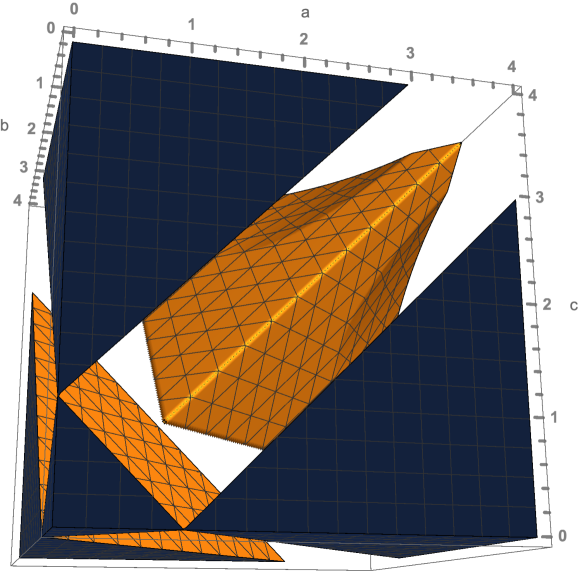
a Regions of known complexity in the eight-vertex model. The four corner regions constitute $\mathcal{F}_{>}$. The non-corner region depicted is $\mathcal{F}_{\leq^{2}}\bigcap\mathcal{A}_{\leq}\bigcap\mathcal{B}_{\leq}\bigcap\mathcal{C}_{\leq}$.

b An extra region that admits FPRAS on planar graphs.

Figure 2:

To prove the FPRAS result in Theorem 1.1, our most important contribution is a set of closure properties. We prove these closure properties for the eight-vertex model in Section 3. We then use these closure properties to show that a Markov chain designed for the six-vertex model can be adapted to provide our FPRAS. The Markov chain we adapt is the directed-loop algorithm which was invented by Rahman and Stillinger [RS72] and is widely used for the six-vertex model (e.g., [YN79, BN98, SZ04]). The state space of our Markov chain for the eight-vertex model consists of even orientations and near-even orientations, which is an extension of the space of valid configurations; the transitions of this algorithm are composed of creating, shifting, and merging of two “defective” edges. A formal description of the directed-loop algorithm is given in Section 4.

This leads to a Markov chain Monte Carlo approximate counting algorithm by sampling. To prove that this is an FPRAS, we show that (1) the above Markov chain is rapidly mixing via a conductance argument [JS89, DFK91, Sin92, Jer03], (2) the valid configurations take a non-negligible proportion in the state space, and (3) there is a (not totally obvious) self-reduction (to reduce the computation of the partition function of a graph to that of a “smaller” graph) [JVV86]. All three parts depend on the closure properties. Specifically, we show that when $(a,b,c,d)\in\mathcal{F}_{\leq^{2}}$, the conductance of the Markov chain can be polynomially bounded if the ratio of near-even orientations over even orientations can be polynomially bounded; when $(a,b,c,d)\in\mathcal{A}_{\leq}\bigcap\mathcal{B}_{\leq}\bigcap\mathcal{C}_{\leq}$, this ratio is indeed polynomially bounded according to the closure properties. Finally a self-reduction whose success in $\mathcal{A}_{\leq}\bigcap\mathcal{B}_{\leq}\bigcap\mathcal{C}_{\leq}$ requires an additional closure property. Therefore, there is an FPRAS in the intersection of $\mathcal{F}_{\leq^{2}}$ and $\mathcal{A}_{\leq}\bigcap\mathcal{B}_{\leq}\bigcap\mathcal{C}_{\leq}$.

The closure properties are keys to our FPRAS. We use the term a 4-ary construction to denote a 4-regular graph $\Gamma$ having four “dangling” edges, and consider all configurations on the edges of $\Gamma$ where every vertex satisfies the even orientation rule and has arrow reversal symmetry. We can prove that this $\Gamma$ defines a constraint function of arity 4 that also satisfies the even orientation rule and has arrow reversal symmetry. If we imagine the graph $\Gamma$ is shrunken to a single point except the 4 dangling edges, then a 4-ary construction can be viewed as a virtual vertex with parameters $(a^{\prime},b^{\prime},c^{\prime},d^{\prime})$ in the eight-vertex model, for some $a^{\prime},b^{\prime},c^{\prime},d^{\prime}\geq 0$.

In Theorem 3.2 we show that the set of 4-ary constraint functions in $\mathcal{A}_{\leq}\bigcap\mathcal{B}_{\leq}\bigcap\mathcal{C}_{\leq}$ is closed under 4-ary constructions. This is achieved by inventing a “quantum decomposition” of even-orientations. In [CLL19] a special case of Theorem 3.2 when $d=0$ is proved for the six-vertex model using a decomposition of Eulerian orientations. Given $G=(V,E)$, every Eulerian orientation defines a set of $2^{|V|}$ directed Eulerian partitions by pairing up the four edges around a vertex in one of two ways such that each pair of edges satisfies “1-in-1-out”. However, such a decomposition does not exist when sinks and sources appear in the eight-vertex model.

In order to overcome this difficulty, we introduce a quantum decomposition where each vertex has a “signed” pairing. Given an even orientation, a plus pairing groups the four edges around a vertex into two pairs such that both pairs satisfy “1-in-1-out”; a minus pairing groups the four edges around a vertex into two pairs such that both pairs independently satisfy either “2-in” or “2-out”. With weights, this gives rise to a quantum decomposition of $3^{|V|}$ “annotated” circuit partitions. (Details are in Section 3.) Although the idea of “pairings” and decompositions of Eulerian orientations have been used before [Ver88, Jae90, MW96], the idea of a signed pairing and the associated quantum decomposition of even orientations into annotated circuit partitions is new. Just as statistical physicists introduce the eight-vertex model on the square lattice for certain desirable properties and better universality over the six-vertex model, in approximate complexity on 4-regular graphs our technique that gives FPRAS for the eight-vertex model extends significantly beyond those for the six-vertex model.

Not only more sophisticated techniques are needed, the landscape of approximate complexity for the eight-vertex model is also richer. In the six-vertex model we have $d=0$. Then it follows that $\mathcal{F}_{\leq^{2}}\subset\mathcal{A}_{\leq}\bigcap\mathcal{B}_{\leq}\bigcap\mathcal{C}_{\leq}$ which means whenever the conductance of the directed-loop algorithm can be bounded by the ratio of near-even orientations over even orientations, there is an FPRAS. In the eight-vertex model, however, there are parameter settings in $\mathcal{F}_{\leq^{2}}$ where the ratio can be exponentially large. This indicates that the current MCMC method is unable to give FPRAS for the whole region $\mathcal{F}_{\leq^{2}}$, even though there is a nice upper bound for the conductance of this Markov chain.

Moreover, in the eight-vertex model we can give more positive results for planar graphs than for general graphs, unlike in the six-vertex model whenever we have an FPRAS for planar graphs we also have one for general graphs for the same parameters. For planar graphs, in Theorem 3.3 and Corollary 3.4 we show that the extra regions $\mathcal{A}_{\leq}\bigcap\mathcal{B}_{\leq}\bigcap\mathcal{C}_{\geq}\bigcap\overline{\mathcal{F}_{>}}$ and $\mathcal{A}_{\leq}\bigcap\mathcal{B}_{\leq}\bigcap\mathcal{C}_{=}$ also enjoy closure properties. It turns out that (only) on planar graphs we have an FPRAS when the parameter setting is in the intersection of $\mathcal{A}_{\leq}\bigcap\mathcal{B}_{\leq}\bigcap\mathcal{C}_{\geq}\bigcap\overline{\mathcal{F}_{>}}$ and $\mathcal{F}_{\leq^{2}}$. And since $\mathcal{F}_{\leq^{2}}\subset\overline{\mathcal{F}_{>}}$, combined with the FPRAS on general graphs, we get an FPRAS for $\mathcal{F}_{\leq^{2}}\bigcap\mathcal{A}_{\leq}\bigcap\mathcal{B}_{\leq}$ for all planar graphs. This tolerance of dropping off the requirement $c+d\leq a+b$ is in perfect accordance with the special role that “saddle” configurations (Figure 1-5 and Figure 1-6) play on planar graphs. Although this region is disjoint from the hard regions on general graphs, we find this region is FPRASable on planar graphs but its approximate complexity is unknown for general graphs. Considering the fact that the exact complexity for the eight-vertex model on planar graphs is not even understood, this is one of the very few cases where research on approximate complexity has advanced beyond that on exact complexity.

The NP-hardness of approximation in FE&AFE regions is shown by reductions from the problem of computing the maximum cut on a 3-regular graph. For the eight-vertex models not included in the six-vertex model ($d\neq 0$), both the reduction source and the “gadgets” we employ to prove the hardness are substantially different from those that were used in the hardness proof of the six-vertex model [CLL19]. We note that the parameter settings in [GR10] where torpid mixing is proved are contained in our NP-hardness region.

In addition to the complexity result, we show that there is a fundamental difference in the behavior on the two sides separated by the phase transition threshold, in terms of closure properties. In Theorem 3.1, we show that the set of 4-ary constraint functions lying in the complement of $\mathcal{F}_{>}$ is closed under 4-ary constructions. We prove in this paper that approximation is hard on $\mathcal{F}_{>}$. It is not known if the eight-vertex model in the full region of $\overline{\mathcal{F}_{>}}$ admits FPRAS or not.

The eight-vertex model fits into the wider class of Holant problems and serves as important basic cases for the latter. Previous results in approximate counting are mostly about spin systems and the present paper, together with [CLL19], are probably the first fruitful attempts in the Holant literature to make connections to phase transitions. While there is still a gap in the complexity picture for the six-vertex and eight-vertex models, we believe the framework set in this paper gives a starting point for studying the approximation complexity of a broader class of counting problems.

2 Preliminaries

Given a 4-regular graph $G=(V,E)$, the edge-vertex incidence graph $G^{\prime}=(U_{E},U_{V},E^{\prime})$ is a bipartite graph where $(u_{e},u_{v})\in U_{E}\times U_{V}$ is an edge in $E^{\prime}$ iff $e\in E$ in $G$ is incident to $v\in V$. We model an orientation ($w\rightarrow v$) on an edge $e=\left\{w,v\right\}\in E$ from $w$ into $v$ in $G$ by assigning $1$ to $(u_{e},u_{w})\in E^{\prime}$ and $0$ to $(u_{e},u_{v})\in E^{\prime}$ in $G^{\prime}$. A configuration of the eight-vertex model on $G$ is an edge 2-coloring on $G^{\prime}$, namely $\sigma:E^{\prime}\rightarrow\{0,1\}$, where for each $u_{e}\in U_{E}$ its two incident edges are assigned 01 or 10, and for each $u_{v}\in U_{V}$ the sum of values $\sum_{i=1}^{4}\sigma(e_{i})\equiv 0\pmod{2}$, over the four incident edges of $u_{v}$. Thus we model the even orientation rule of $G$ on all $v\in V$ by requiring “two-0-two-1/four-0/four-1” locally at each vertex $u_{v}\in U_{V}$.

The “one-0-one-1” requirement on the two edges incident to a vertex in $U_{E}$ is a binary Disequality constraint, denoted by $(\neq_{2})$. The values of a 4-ary constraint function $f$ can be listed in a matrix $M(f)=\left[\begin{smallmatrix}f_{0000}&f_{0010}&f_{0001}&f_{0011}\\ f_{0100}&f_{0110}&f_{0101}&f_{0111}\\ f_{1000}&f_{1010}&f_{1001}&f_{1011}\\ f_{1100}&f_{1110}&f_{1101}&f_{1111}\end{smallmatrix}\right]$, called the constraint matrix of $f$. For the eight-vertex model satisfying the even orientation rule and arrow reversal symmetry, the constraint function $f$ at every vertex $v\in U_{V}$ in $G^{\prime}$ has the form $M(f)=\left[\begin{smallmatrix}d&0&0&a\\ 0&b&c&0\\ 0&c&b&0\\ a&0&0&d\end{smallmatrix}\right]$, if we locally index the left, down, right, and up edges incident to $v$ by 1, 2, 3, and 4, respectively according to Figure 1. Thus computing the partition function $Z(G;a,b,c,d)$ is equivalent to evaluating (the Holant sum in the framework for Holant problems)

$$Z^{\prime}(G^{\prime};f):=\sum_{\sigma:E^{\prime}\rightarrow\left\{0,1\right\}}\prod_{u\in U_{E}}(\neq_{2})\left(\sigma|_{E^{\prime}(u)}\right)\prod_{u\in U_{V}}f\left(\sigma|_{E^{\prime}(u)}\right).$$

where $E^{\prime}(u)$ denotes the incident edges of $u\in U_{E}\cup U_{V}$.

When every vertex in $G$ has the same constraint function $f$ with $M(f)=\left[\begin{smallmatrix}d&&&a\\ &b&c&\\ &c&b&\\ a&&&d\end{smallmatrix}\right]$, we write the partition function $Z(a,b,c,d)$ as $Z(f)$, and denote by $Z(\mathcal{F})$ when each vertex is assigned some constraint function from a set $\mathcal{F}$ consisting of constraint functions of this form.

3 Closure Properties

Theorem 3.1.

The set of constraint functions in $\overline{\mathcal{F}_{>}}$ is closed under 4-ary constructions, i.e., the constraint function of any 4-ary construction using constraint functions from the set $\overline{\mathcal{F}_{>}}$ also belongs to the same set.

Theorem 3.2.

The set of constraint functions in $\mathcal{A}_{\leq}\bigcap\mathcal{B}_{\leq}\bigcap\mathcal{C}_{\leq}$ is closed under 4-ary constructions.

Theorem 3.3.

The set of constraint functions in $\mathcal{A}_{\leq}\bigcap\mathcal{B}_{\leq}\bigcap\mathcal{C}_{\geq}\bigcap\overline{\mathcal{F}_{>}}$ is closed under 4-ary plane constructions.

Corollary 3.4.

The set of constraint functions in $\mathcal{A}_{\leq}\bigcap\mathcal{B}_{\leq}\bigcap\mathcal{C}_{=}$ is closed under 4-ary plane constructions.

In order to prove the above closure properties, we introduce a quantum decomposition for the eight-vertex model, in which every even orientation of a 4-regular graph $G=(V,E)$ is a “superposition” of $3^{|V|}$ annotated circuit partitions (to be defined shortly).

Let $v$ be a vertex of $G$, and $e_{1},e_{2},e_{3},e_{4}$ the four labeled edges incident to $v$. A pairing $\varrho$ at $v$ is a partition of $\{e_{1},e_{2},e_{3},e_{4}\}$ into two pairs. There are exactly three distinct pairings at $v$ (Figure 3) which we denote by three special symbols: $\raisebox{-1.20007pt}{\includegraphics[height=8.39996pt,width=8.39996pt,keepaspectratio]{sub_1}},\raisebox{-1.20007pt}{\includegraphics[height=8.39996pt,width=8.39996pt,keepaspectratio]{sub_2}},\raisebox{-1.20007pt}{\includegraphics[height=8.39996pt,width=8.39996pt,keepaspectratio]{sub_3}}$, respectively. A circuit partition of a graph $G$ is a partition of the edges of $G$ into edge-disjoint circuits (in such a circuit vertices may repeat but edges may not). It is in 1-1 correspondence with a family of pairings $\varphi=\{\varrho_{v}\}_{v\in V}$, where $\varrho_{v}\in\{\raisebox{-1.20007pt}{\includegraphics[height=8.39996pt,width=8.39996pt,keepaspectratio]{sub_1}},\raisebox{-1.20007pt}{\includegraphics[height=8.39996pt,width=8.39996pt,keepaspectratio]{sub_2}},\raisebox{-1.20007pt}{\includegraphics[height=8.39996pt,width=8.39996pt,keepaspectratio]{sub_3}}\}$ is a pairing at $v$—once the pairing at each vertex is fixed, then the two edges paired together at each vertex is also adjacent in the same circuit.

a

b

c

Figure 3: (Unsigned) pairings at a degree 4 vertex.

A signed pairing $\boldsymbol{\varrho}_{v}$ at $v$ is a pairing with a sign, either plus ($+$) or minus ($-$). In other words, it is an element in $\{\raisebox{-1.20007pt}{\includegraphics[height=8.39996pt,width=8.39996pt,keepaspectratio]{sub_1}},\raisebox{-1.20007pt}{\includegraphics[height=8.39996pt,width=8.39996pt,keepaspectratio]{sub_2}},\raisebox{-1.20007pt}{\includegraphics[height=8.39996pt,width=8.39996pt,keepaspectratio]{sub_3}}\}\times\{+,-\}$. We denote a signed pairing by $\varrho_{+}$ or $\varrho_{-}$ if the pairing is $\varrho$ and the sign is plus or minus, respectively. An annotated circuit partition of $G$, or acp for short, is a circuit partition of $G$ together with a map $V\rightarrow\{+,-\}$ such that along every circuit one encounters an even number of $-$ (a repeat vertex with $-$ counts twice on the circuit). Thus, it is in 1-1 correspondence with a family of signed pairings for all $v\in V$, with the restriction that there is an even number of $-$ along each circuit. Each circuit $C$ in an acp has exactly two directed states—starting at an arbitrary edge in $C$ with one of the two orientations on this edge, one can uniquely orient every edge in $C$ such that for every vertex $v$ on $C$, two edges incident at $v$ paired up by $+$ have consistent orientations at $v$ (i.e., they form “1-in-1-out” at $v$), whereas two edges paired up by $-$ have contrary orientations at $v$ (i.e., they form “2-in” or “2-out” at $v$). These two directed states of $C$ are well-defined because cyclically the direction of edges along $C$ changes an even number of times, precisely at the minus signs. A directed annotated circuit partition (dacp) is an acp with each circuit in a directed state. If an acp has $k$ circuits, then it defines $2^{k}$ dacp’s.

Next we describe an association between even orientations and acp’s as well as dacp’s. Given an even orientation $\tau$ of $G$, every local configuration of $\tau$ at a vertex defines exactly three signed pairings at this vertex according to Table 1. Note that, given $\tau$ and a pairing at a vertex $v$, the two pairs have either both consistent or both contrary orientations. Thus the same sign, $+$ or $-$, works for both pairs, although this depends on the pairing at $v$.

Table 1: Map from eight local configurations to signed pairings.

Configurations		Weight		Sign
		$a$		-	+	+
		$b$		+	-	+
		$c$		+	+	-
		$d$		-	-	-

In this way, every even orientation $\tau$ defines $3^{|V|}$ acp’s, denoted by $\Phi(\tau)$. See Table 2 and Table 3 for two examples. Moreover, for any acp $\varphi\in\Phi(\tau)$, every circuit in $\varphi$ is in one of the two well-defined directed states under the orientation $\tau$. Thus each even orientation $\tau$ defines $3^{|V|}$ dacp’s.

Table 2: An even orientation and its quantum decomposition into acp’s.

$\tau$ abcdefg	$\Phi(\tau)$
abcdefg
abcdefg
abcdefg
abcdefg
abcdefg
abcdefg
abcdefg

Table 3: Another even orientation and its quantum decomposition into acp’s.

$\tau$ abcdefg	$\Phi(\tau)$
abcdefg
abcdefg
abcdefg
abcdefg
abcdefg
abcdefg
abcdefg

Conversely, for any dacp, if we ignore the signs at all vertices we get a valid even orientation (because each sign applies to both pairs). If a dacp comes from $\Phi(\tau)$ then we get back the even orientation $\tau$. Therefore, the association from even orientations to dacp’s is $1$-to-$3^{|V|}$, non-overlapping, and surjective. Define $w$ to be a function assigning a weight to every signed pairing at every vertex and let the weight $\tilde{w}(\varphi)$ of an annotated circuit partition $\varphi$, either undirected (acp) or directed (dacp), be the product of weights at each vertex. For every vertex in the eight-vertex model with the parameter setting $(a,b,c,d)$, we define $w$ such that

$$\left\{\begin{smallmatrix}a=w(\raisebox{-1.20007pt}{\includegraphics[height=12.0pt,width=12.0pt,keepaspectratio]{sub_1}}_{-})+w(\raisebox{-1.20007pt}{\includegraphics[height=12.0pt,width=12.0pt,keepaspectratio]{sub_2}}_{+})+w(\raisebox{-1.20007pt}{\includegraphics[height=12.0pt,width=12.0pt,keepaspectratio]{sub_3}}_{+})\\ b=w(\raisebox{-1.20007pt}{\includegraphics[height=12.0pt,width=12.0pt,keepaspectratio]{sub_1}}_{+})+w(\raisebox{-1.20007pt}{\includegraphics[height=12.0pt,width=12.0pt,keepaspectratio]{sub_2}}_{-})+w(\raisebox{-1.20007pt}{\includegraphics[height=12.0pt,width=12.0pt,keepaspectratio]{sub_3}}_{+})\\ c=w(\raisebox{-1.20007pt}{\includegraphics[height=12.0pt,width=12.0pt,keepaspectratio]{sub_1}}_{+})+w(\raisebox{-1.20007pt}{\includegraphics[height=12.0pt,width=12.0pt,keepaspectratio]{sub_2}}_{+})+w(\raisebox{-1.20007pt}{\includegraphics[height=12.0pt,width=12.0pt,keepaspectratio]{sub_3}}_{-})\\ d=w(\raisebox{-1.20007pt}{\includegraphics[height=12.0pt,width=12.0pt,keepaspectratio]{sub_1}}_{-})+w(\raisebox{-1.20007pt}{\includegraphics[height=12.0pt,width=12.0pt,keepaspectratio]{sub_2}}_{-})+w(\raisebox{-1.20007pt}{\includegraphics[height=12.0pt,width=12.0pt,keepaspectratio]{sub_3}}_{-})\\ \end{smallmatrix}\right..$$ (3.1)

Note that for any $a,b,c,d$ this is a linear system of rank 4 in six variables, and there is a solution space of dimension 2 (Lemma 3.7 discusses this freedom). Then the weight of an eight-vertex model configuration $\tau$ is equal to $\sum_{\varphi\in\Phi(\tau)}\tilde{w}(\varphi)$. This is obtained by writing a term in the summation in (1.1), which is a product of sums by (3.1), as a sum of products. Note that a single acp has the same weight when it becomes directed regardless which directed state the dacp is in.

We will illustrate the above in detail by the examples in Table 2 and Table 3. We assume the same constraint $(a,b,c,d)$ is applied at $u$ and $v$. The orientation at one vertex determines the other in this graph $G$. There are a total 8 valid configurations, 4 of which are total reversals of the other 4. $Z(G)=2[a^{2}+b^{2}+c^{2}+d^{2}]$. When we expand $Z(G)$ using (3.1) we get a total of 72 terms. These correspond to 72 dacp’s. There are 9 ways to assign a pairing at $u$ and at $v$. If we consider the configuration in Table 2, these 9 ways are listed under $\Phi(\tau)$, where the local orientation also determines a sign $\pm$ at both $u$ and $v$. These are 9 acp’s (without direction). For each acp $\varphi$, the weight $\tilde{w}(\varphi)$ is defined (without referring to the dacp, or the state of orientation on these circuits). Three of the acp’s (in the diagonal positions) define two distinct circuits while the other six define one circuit each. For each 2-tuple of pairings $(\rho_{u},\rho_{v})$ that results in two circuits, the only valid annotations assign $(+,+)$ or $(-,-)$ at $(u,v)$, giving a total of 6 acp’s. And since each has two circuits, there are a total of $24$ dacp’s. For the other six (off-diagonal) 2-tuples of pairings $(\rho_{u},\rho_{v})$ that results in a single circuit, each has 4 valid annotations, giving a total of 24 acp’s. But these have only one circuit and thus give 48 dacp’s. To appreciate the “quantum superposition” of the decomposition, note that the same acp that has $(\raisebox{-1.20007pt}{\includegraphics[height=8.39996pt,width=8.39996pt,keepaspectratio]{sub_2}}_{+},\raisebox{-1.20007pt}{\includegraphics[height=8.39996pt,width=8.39996pt,keepaspectratio]{sub_2}}_{+})$ at $(u,v)$ appears in both decompositions for the distinct configurations in Table 2 and Table 3.

Remark 3.1.

While a weight function $w$ satisfying (3.1) is not unique, there are some regions of $(a,b,c,d)$ that can be specified directly in terms of $w$ by any weight function $w$ satisfying (3.1), and the specification is independent of the choice of the weight function. E.g., the region $\overline{\mathcal{F}_{>}}$ is specified by $\left\{\begin{smallmatrix}w(\raisebox{-1.20007pt}{\includegraphics[height=12.0pt,width=12.0pt,keepaspectratio]{sub_1}}_{+})+w(\raisebox{-1.20007pt}{\includegraphics[height=12.0pt,width=12.0pt,keepaspectratio]{sub_2}}_{-})+w(\raisebox{-1.20007pt}{\includegraphics[height=12.0pt,width=12.0pt,keepaspectratio]{sub_3}}_{-})\geq 0\\ w(\raisebox{-1.20007pt}{\includegraphics[height=12.0pt,width=12.0pt,keepaspectratio]{sub_1}}_{-})+w(\raisebox{-1.20007pt}{\includegraphics[height=12.0pt,width=12.0pt,keepaspectratio]{sub_2}}_{+})+w(\raisebox{-1.20007pt}{\includegraphics[height=12.0pt,width=12.0pt,keepaspectratio]{sub_3}}_{-})\geq 0\\ w(\raisebox{-1.20007pt}{\includegraphics[height=12.0pt,width=12.0pt,keepaspectratio]{sub_1}}_{-})+w(\raisebox{-1.20007pt}{\includegraphics[height=12.0pt,width=12.0pt,keepaspectratio]{sub_2}}_{-})+w(\raisebox{-1.20007pt}{\includegraphics[height=12.0pt,width=12.0pt,keepaspectratio]{sub_3}}_{+})\geq 0\\ w(\raisebox{-1.20007pt}{\includegraphics[height=12.0pt,width=12.0pt,keepaspectratio]{sub_1}}_{+})+w(\raisebox{-1.20007pt}{\includegraphics[height=12.0pt,width=12.0pt,keepaspectratio]{sub_2}}_{+})+w(\raisebox{-1.20007pt}{\includegraphics[height=12.0pt,width=12.0pt,keepaspectratio]{sub_3}}_{+})\geq 0\\ \end{smallmatrix}\right.$. Also $\mathcal{A}_{\leq}$ is specified by $w(\raisebox{-1.20007pt}{\includegraphics[height=8.39996pt,width=8.39996pt,keepaspectratio]{sub_1}}_{-})\leq w(\raisebox{-1.20007pt}{\includegraphics[height=8.39996pt,width=8.39996pt,keepaspectratio]{sub_1}}_{+})$, $\mathcal{B}_{\leq}$ by $w(\raisebox{-1.20007pt}{\includegraphics[height=8.39996pt,width=8.39996pt,keepaspectratio]{sub_2}}_{-})\leq w(\raisebox{-1.20007pt}{\includegraphics[height=8.39996pt,width=8.39996pt,keepaspectratio]{sub_2}}_{+})$, and $\mathcal{C}_{\leq}$ by $w(\raisebox{-1.20007pt}{\includegraphics[height=8.39996pt,width=8.39996pt,keepaspectratio]{sub_3}}_{-})\leq w(\raisebox{-1.20007pt}{\includegraphics[height=8.39996pt,width=8.39996pt,keepaspectratio]{sub_3}}_{+})$. In Lemma 3.7, we will show that a nonnegative weight function $w$ satisfying (3.1) exists iff $(a,b,c,d)\in\overline{\mathcal{F}_{>}}$.

Remark 3.2.

Although the association from even orientations to dacp’s is $1$-to-$3^{|V|}$, non-overlapping, and surjective, the association from even orientations to acp’s is overlapping. If an acp has $k$ circuits, it will be associated with $2^{k}$ even orientations. It is this many-to-many association, with corresponding weights, between even orientations and acp’s, that we call a quantum decomposition of eight-vertex model configurations, and each is expressed as a “superposition” (weighted sum) of acp’s.

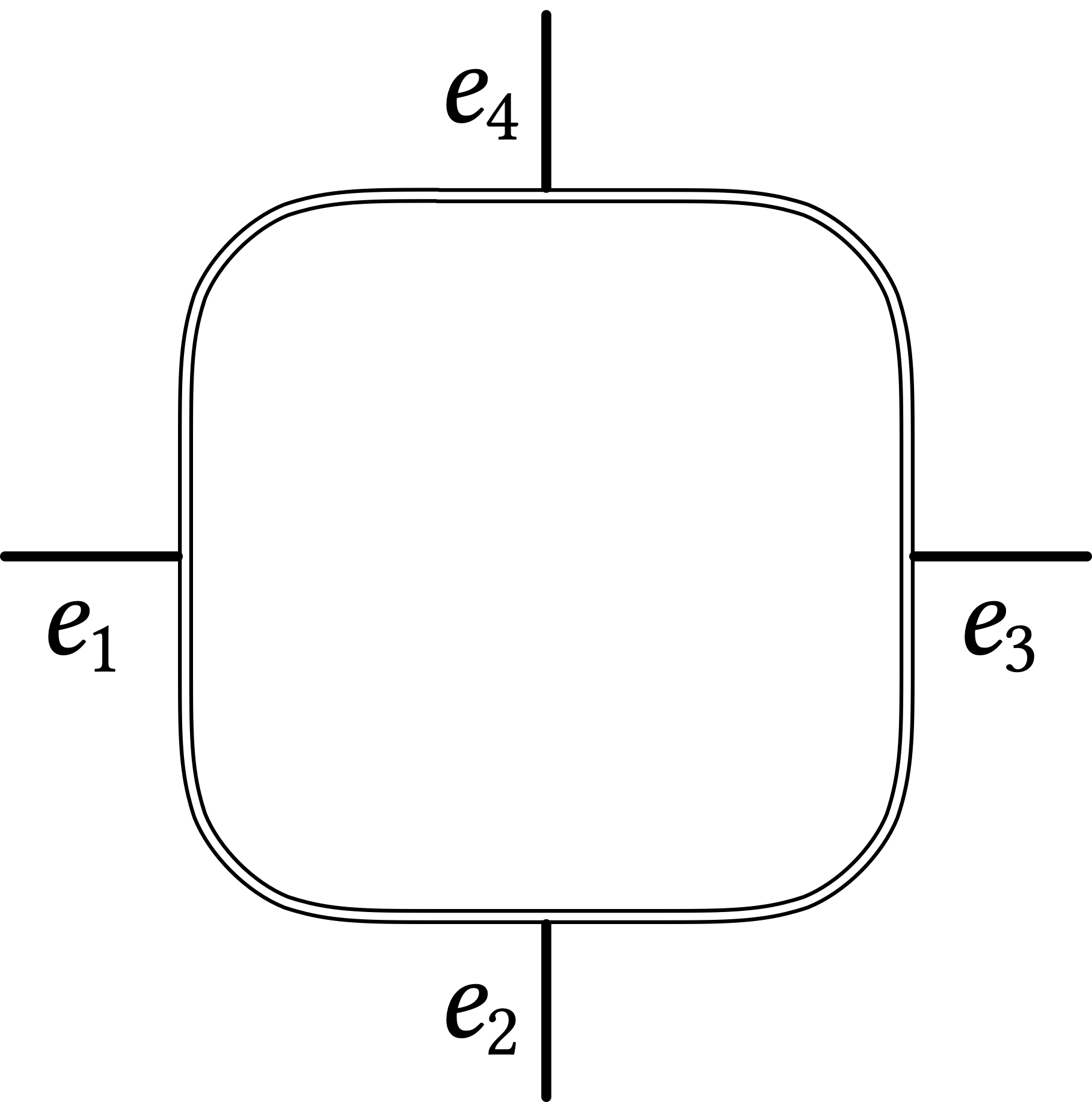
a

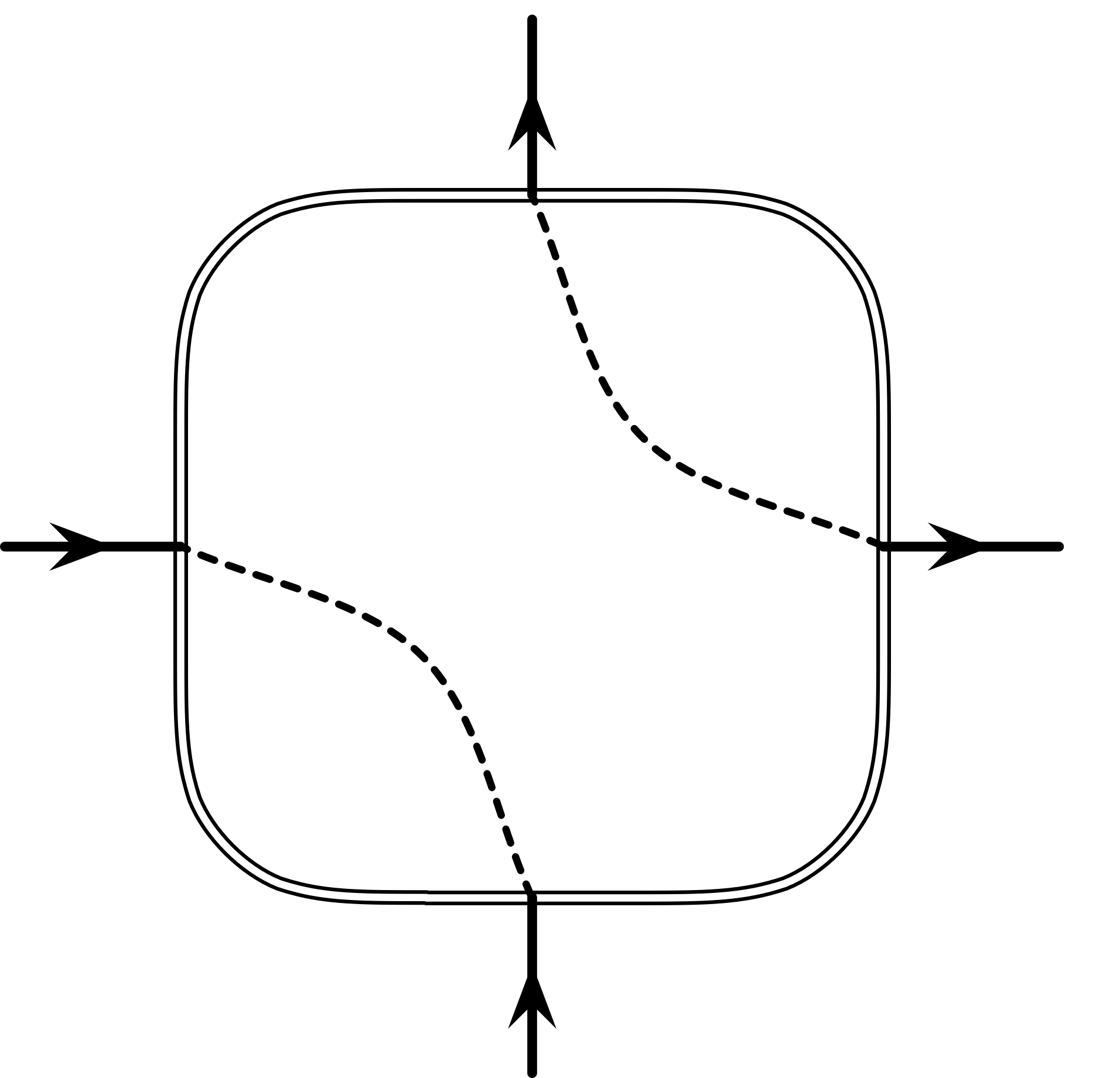
b

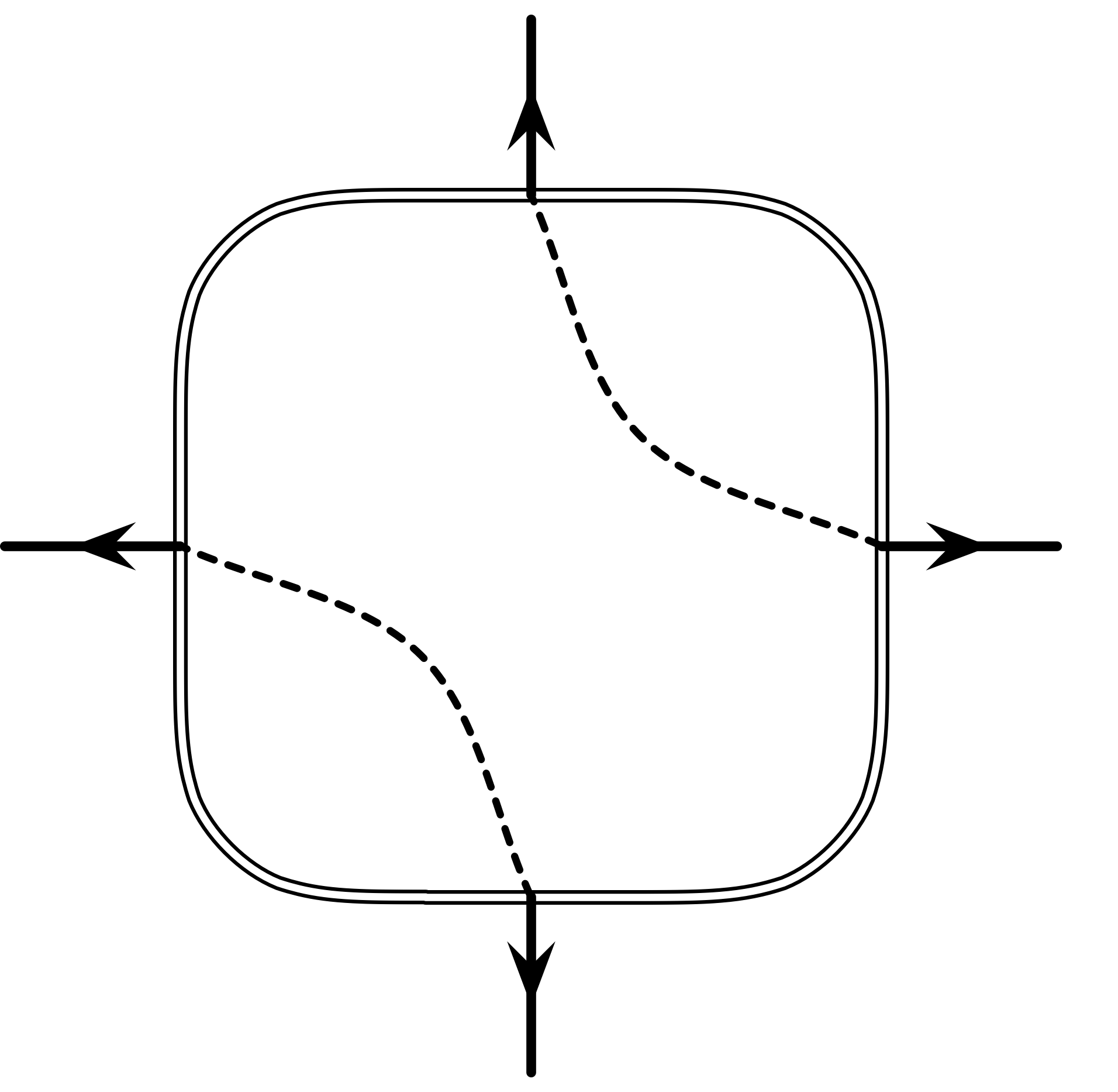
c

Figure 4: A 4-ary construction in the eight-vertex model.

A 4-ary construction is a 4-regular graph $\Gamma$ having four “dangling” edges (Figure 4a), and a constraint function on each node. It defines a 4-ary constraint function with these four dangling edges as input variables, when we sum the product of constraint function values on all vertices, over all configurations on the internal edges of $\Gamma$. If we imagine the graph $\Gamma$ is shrunken to a single point except the 4 dangling edges, then a 4-ary construction can be viewed as a virtual vertex with parameters $(a^{\prime},b^{\prime},c^{\prime},d^{\prime})$ in the eight-vertex model, for some $a^{\prime},b^{\prime},c^{\prime},d^{\prime}\geq 0$. This is proved in the following lemma. A planar 4-ary construction is a 4-regular plane graph with four dangling edges on the outer face ordered counterclockwise $e_{1},e_{2},e_{3},e_{4}$.

Lemma 3.5.

If constraint functions in $\Gamma$ satisfy the even orientation rule and have arrow reversal symmetry, then the constraint function $f$ defined by $\Gamma$ also satisfies the even orientation rule and has arrow reversal symmetry.

Proof.

Consider any even orientation on $\Gamma$, and let $\Delta$ be the (sum of all in-degrees) $-$ (the sum of all out-degrees). Each internal edge contrutes 0 to $\Delta$. By the even orientation rule, at every vertex this difference is $0\pmod{4}$. Thus $\Delta\equiv 0\pmod{4}$. Thus among the dangling edges, it also satisfies the even orientation rule.

If we reverse all directions of an even orientation, which is an involution, each vertex contributes the same weight by arrow reversal symmetry. Hence $f$ also has the arrow reversal symmetry. ∎

A trail & circuit partition (tcp) for a 4-ary construction $\Gamma$ is a partition of the edges in $\Gamma$ into edge-disjoint circuits and exactly two trails (walks with no repeated edges) which end in the four dangling edges. An annotated trail & circuit partition (atcp) for $\Gamma$ is a tcp with a valid annotation, which assigns an even number of $-$ sign along each circuit. Like circuits, each trail in an atcp has exactly two directed states. If an atcp $\varphi$ has $k$ circuits (and $2$ trails), then $\varphi$ defines $2^{k+2}$ directed annotated trail & circuit partitions (datcp’s). The weight $\tilde{w}(\varphi)$ of an annotated trail & circuit partition $\varphi$, either an atcp or datcp, can be similarly defined. Again set the weight function as in (3.1).

Denote the constraint function of $\Gamma$ by $f$ and use the notations introduced in Section 2. Consider $f(0011)$. Under the eight-vertex model, if a configuration $\tau$ of the 4-ary construction with constraint function $f$ has a nonzero contribution to $f(0011)$, it has $e_{1},e_{2}$ coming in and $e_{3},e_{4}$ going out. The contribution by $\tau$ is a weighted sum over a set $\Phi_{0011}(\tau)$ of datcp’s. Each datcp in $\Phi_{0011}(\tau)$ is captured in exactly one of the following three types, according to how $e_{1},e_{2},e_{3},e_{4}$ are connected by the two trails:

1. $\{\ \xrightarrow{e_{1}}\Square\xleftarrow{e_{2}},~{}\xleftarrow{e_{3}}\Square\xrightarrow{e_{4}}\}$ and on both trails the numbers of minus pairings are odd; or

2. $\{\ \xrightarrow{e_{1}}\Square\xrightarrow{e_{4}},~{}\xrightarrow{e_{2}}\Square\xrightarrow{e_{3}}\}$ and on both trails the numbers of minus pairings are even (Figure 4b); or

3. $\{\ \xrightarrow{e_{1}}\Square\xrightarrow{e_{3}},~{}\xrightarrow{e_{2}}\Square\xrightarrow{e_{4}}\}$ and on both trails the numbers of minus pairings are even.

Let $\Phi_{0011,\raisebox{-1.20007pt}{\includegraphics[height=8.39996pt,width=8.39996pt,keepaspectratio]{sub_1}}_{-}}$, $\Phi_{0011,\raisebox{-1.20007pt}{\includegraphics[height=8.39996pt,width=8.39996pt,keepaspectratio]{sub_2}}_{+}}$ and $\Phi_{0011,\raisebox{-1.20007pt}{\includegraphics[height=8.39996pt,width=8.39996pt,keepaspectratio]{sub_3}}_{+}}$ be the subsets of datcp’s contributing to $f(0011)$ defined in case (1), (2) and (3) respectively. The value $f(0011)$ is a weighted sum of contributions according to $\tilde{w}$ from these three disjoint sets. Defining the weight of a set $\Phi$ of datcp’s by $W(\Phi)=\sum_{\varphi\in\Phi}\tilde{w}(\varphi)$ yields $f(0011)=W(\Phi_{0011,\raisebox{-1.20007pt}{\includegraphics[height=8.39996pt,width=8.39996pt,keepaspectratio]{sub_1}}_{-}})+W(\Phi_{0011,\raisebox{-1.20007pt}{\includegraphics[height=8.39996pt,width=8.39996pt,keepaspectratio]{sub_2}}_{+}})+W(\Phi_{0011,\raisebox{-1.20007pt}{\includegraphics[height=8.39996pt,width=8.39996pt,keepaspectratio]{sub_3}}_{+}})$. Similarly we can define $\Phi_{1100,\raisebox{-1.20007pt}{\includegraphics[height=8.39996pt,width=8.39996pt,keepaspectratio]{sub_1}}_{-}},\Phi_{1100,\raisebox{-1.20007pt}{\includegraphics[height=8.39996pt,width=8.39996pt,keepaspectratio]{sub_2}}_{+}}$ and $\Phi_{1100,\raisebox{-1.20007pt}{\includegraphics[height=8.39996pt,width=8.39996pt,keepaspectratio]{sub_3}}_{+}}$, and get $f(1100)=W(\Phi_{1100,\raisebox{-1.20007pt}{\includegraphics[height=8.39996pt,width=8.39996pt,keepaspectratio]{sub_1}}_{-}})+W(\Phi_{1100,\raisebox{-1.20007pt}{\includegraphics[height=8.39996pt,width=8.39996pt,keepaspectratio]{sub_2}}_{+}})+W(\Phi_{1100,\raisebox{-1.20007pt}{\includegraphics[height=8.39996pt,width=8.39996pt,keepaspectratio]{sub_3}}_{+}})$. Note that there is a bijective weight-preserving map between $\Phi_{0011,\raisebox{-1.20007pt}{\includegraphics[height=8.39996pt,width=8.39996pt,keepaspectratio]{sub_1}}_{-}}$ and $\Phi_{1100,\raisebox{-1.20007pt}{\includegraphics[height=8.39996pt,width=8.39996pt,keepaspectratio]{sub_1}}_{-}}$ by reversing the direction of every circuit and trail of a datcp. Thus, $W(\Phi_{0011,\raisebox{-1.20007pt}{\includegraphics[height=8.39996pt,width=8.39996pt,keepaspectratio]{sub_1}}_{-}})=W(\Phi_{1100,\raisebox{-1.20007pt}{\includegraphics[height=8.39996pt,width=8.39996pt,keepaspectratio]{sub_1}}_{-}})$, $W(\Phi_{0011,\raisebox{-1.20007pt}{\includegraphics[height=8.39996pt,width=8.39996pt,keepaspectratio]{sub_2}}_{+}})=W(\Phi_{1100,\raisebox{-1.20007pt}{\includegraphics[height=8.39996pt,width=8.39996pt,keepaspectratio]{sub_2}}_{+}})$, and $W(\Phi_{0011,\raisebox{-1.20007pt}{\includegraphics[height=8.39996pt,width=8.39996pt,keepaspectratio]{sub_3}}_{+}})=W(\Phi_{1100,\raisebox{-1.20007pt}{\includegraphics[height=8.39996pt,width=8.39996pt,keepaspectratio]{sub_3}}_{+}})$. Consequently $f(0011)=f(1100)$. Similarly we have $f(0110)=f(1001)$, $f(0101)=f(1010)$ and $f(0000)=f(1111)$.

For any pairing $\varrho$, and for every 4-bit pattern $b_{1}b_{2}b_{3}b_{4}\in\{0,1\}^{4}$, we can define $\Phi_{b_{1}b_{2}b_{3}b_{4},\varrho_{+}}$ if (both) paired $b_{i}\not=b_{j}$, and $\Phi_{b_{1}b_{2}b_{3}b_{4},\varrho_{-}}$ if (both) paired $b_{i}=b_{j}$. Then a further important observation is that for each datcp in $\Phi_{0011,\raisebox{-1.20007pt}{\includegraphics[height=8.39996pt,width=8.39996pt,keepaspectratio]{sub_1}}_{-}}$, if we only reverse every edge in the trail between $\ \xrightarrow{e_{1}}\Square\xleftarrow{e_{2}}\$ and keep the states of all circuits and the other trail unchanged, this datcp has the same weight but now lies in $\Phi_{1111,\raisebox{-1.20007pt}{\includegraphics[height=8.39996pt,width=8.39996pt,keepaspectratio]{sub_1}}_{-}}$. This is because at every vertex $v$, reversing the orientation of any one branch of the given (annotated) pairing $\boldsymbol{\varrho}_{v}\in\{\raisebox{-1.20007pt}{\includegraphics[height=8.39996pt,width=8.39996pt,keepaspectratio]{sub_1}},\raisebox{-1.20007pt}{\includegraphics[height=8.39996pt,width=8.39996pt,keepaspectratio]{sub_2}},\raisebox{-1.20007pt}{\includegraphics[height=8.39996pt,width=8.39996pt,keepaspectratio]{sub_3}}\}\times\{+,-\}$ does not change the value $w(\boldsymbol{\varrho}_{v})$. In this way, we set up a one-to-one weight-preserving map between $\Phi_{0011,\raisebox{-1.20007pt}{\includegraphics[height=8.39996pt,width=8.39996pt,keepaspectratio]{sub_1}}_{-}}$ and $\Phi_{1111,\raisebox{-1.20007pt}{\includegraphics[height=8.39996pt,width=8.39996pt,keepaspectratio]{sub_1}}_{-}}$, hence $W(\Phi_{0011,\raisebox{-1.20007pt}{\includegraphics[height=8.39996pt,width=8.39996pt,keepaspectratio]{sub_1}}_{-}})=W(\Phi_{1111,\raisebox{-1.20007pt}{\includegraphics[height=8.39996pt,width=8.39996pt,keepaspectratio]{sub_1}}_{-}})$. Combining the result in the last paragraph we have proved the first item below, and we name its common value $W(\raisebox{-1.20007pt}{\includegraphics[height=8.39996pt,width=8.39996pt,keepaspectratio]{sub_1}}_{-})$. The other items are proved similarly.

• $W(\raisebox{-1.20007pt}{\includegraphics[height=8.39996pt,width=8.39996pt,keepaspectratio]{sub_1}}_{-})=W(\Phi_{0011,\raisebox{-1.20007pt}{\includegraphics[height=8.39996pt,width=8.39996pt,keepaspectratio]{sub_1}}_{-}})=W(\Phi_{1100,\raisebox{-1.20007pt}{\includegraphics[height=8.39996pt,width=8.39996pt,keepaspectratio]{sub_1}}_{-}})=W(\Phi_{0000,\raisebox{-1.20007pt}{\includegraphics[height=8.39996pt,width=8.39996pt,keepaspectratio]{sub_1}}_{-}})=W(\Phi_{1111,\raisebox{-1.20007pt}{\includegraphics[height=8.39996pt,width=8.39996pt,keepaspectratio]{sub_1}}_{-}})$;

• $W(\raisebox{-1.20007pt}{\includegraphics[height=8.39996pt,width=8.39996pt,keepaspectratio]{sub_2}}_{-})=W(\Phi_{0110,\raisebox{-1.20007pt}{\includegraphics[height=8.39996pt,width=8.39996pt,keepaspectratio]{sub_2}}_{-}})=W(\Phi_{1001,\raisebox{-1.20007pt}{\includegraphics[height=8.39996pt,width=8.39996pt,keepaspectratio]{sub_2}}_{-}})=W(\Phi_{0000,\raisebox{-1.20007pt}{\includegraphics[height=8.39996pt,width=8.39996pt,keepaspectratio]{sub_2}}_{-}})=W(\Phi_{1111,\raisebox{-1.20007pt}{\includegraphics[height=8.39996pt,width=8.39996pt,keepaspectratio]{sub_2}}_{-}})$;

• $W(\raisebox{-1.20007pt}{\includegraphics[height=8.39996pt,width=8.39996pt,keepaspectratio]{sub_3}}_{-})=W(\Phi_{0101,\raisebox{-1.20007pt}{\includegraphics[height=8.39996pt,width=8.39996pt,keepaspectratio]{sub_3}}_{-}})=W(\Phi_{1010,\raisebox{-1.20007pt}{\includegraphics[height=8.39996pt,width=8.39996pt,keepaspectratio]{sub_3}}_{-}})=W(\Phi_{0000,\raisebox{-1.20007pt}{\includegraphics[height=8.39996pt,width=8.39996pt,keepaspectratio]{sub_3}}_{-}})=W(\Phi_{1111,\raisebox{-1.20007pt}{\includegraphics[height=8.39996pt,width=8.39996pt,keepaspectratio]{sub_3}}_{-}})$;

• $W(\raisebox{-1.20007pt}{\includegraphics[height=8.39996pt,width=8.39996pt,keepaspectratio]{sub_1}}_{+})=W(\Phi_{0110,\raisebox{-1.20007pt}{\includegraphics[height=8.39996pt,width=8.39996pt,keepaspectratio]{sub_1}}_{+}})=W(\Phi_{1001,\raisebox{-1.20007pt}{\includegraphics[height=8.39996pt,width=8.39996pt,keepaspectratio]{sub_1}}_{+}})=W(\Phi_{0101,\raisebox{-1.20007pt}{\includegraphics[height=8.39996pt,width=8.39996pt,keepaspectratio]{sub_1}}_{+}})=W(\Phi_{1010,\raisebox{-1.20007pt}{\includegraphics[height=8.39996pt,width=8.39996pt,keepaspectratio]{sub_1}}_{+}})$;

• $W(\raisebox{-1.20007pt}{\includegraphics[height=8.39996pt,width=8.39996pt,keepaspectratio]{sub_2}}_{+})=W(\Phi_{0011,\raisebox{-1.20007pt}{\includegraphics[height=8.39996pt,width=8.39996pt,keepaspectratio]{sub_2}}_{+}})=W(\Phi_{1100,\raisebox{-1.20007pt}{\includegraphics[height=8.39996pt,width=8.39996pt,keepaspectratio]{sub_2}}_{+}})=W(\Phi_{0101,\raisebox{-1.20007pt}{\includegraphics[height=8.39996pt,width=8.39996pt,keepaspectratio]{sub_2}}_{+}})=W(\Phi_{1010,\raisebox{-1.20007pt}{\includegraphics[height=8.39996pt,width=8.39996pt,keepaspectratio]{sub_2}}_{+}})$;

• $W(\raisebox{-1.20007pt}{\includegraphics[height=8.39996pt,width=8.39996pt,keepaspectratio]{sub_3}}_{+})=W(\Phi_{0011,\raisebox{-1.20007pt}{\includegraphics[height=8.39996pt,width=8.39996pt,keepaspectratio]{sub_3}}_{+}})=W(\Phi_{1100,\raisebox{-1.20007pt}{\includegraphics[height=8.39996pt,width=8.39996pt,keepaspectratio]{sub_3}}_{+}})=W(\Phi_{0110,\raisebox{-1.20007pt}{\includegraphics[height=8.39996pt,width=8.39996pt,keepaspectratio]{sub_3}}_{+}})=W(\Phi_{1001,\raisebox{-1.20007pt}{\includegraphics[height=8.39996pt,width=8.39996pt,keepaspectratio]{sub_3}}_{+}})$.

Consequently, $f$ has parameters $\left\{\begin{smallmatrix}a^{\prime}=W(\raisebox{-1.20007pt}{\includegraphics[height=12.0pt,width=12.0pt,keepaspectratio]{sub_1}}_{-})+W(\raisebox{-1.20007pt}{\includegraphics[height=12.0pt,width=12.0pt,keepaspectratio]{sub_2}}_{+})+W(\raisebox{-1.20007pt}{\includegraphics[height=12.0pt,width=12.0pt,keepaspectratio]{sub_3}}_{+})\\ b^{\prime}=W(\raisebox{-1.20007pt}{\includegraphics[height=12.0pt,width=12.0pt,keepaspectratio]{sub_1}}_{+})+W(\raisebox{-1.20007pt}{\includegraphics[height=12.0pt,width=12.0pt,keepaspectratio]{sub_2}}_{-})+W(\raisebox{-1.20007pt}{\includegraphics[height=12.0pt,width=12.0pt,keepaspectratio]{sub_3}}_{+})\\ c^{\prime}=W(\raisebox{-1.20007pt}{\includegraphics[height=12.0pt,width=12.0pt,keepaspectratio]{sub_1}}_{+})+W(\raisebox{-1.20007pt}{\includegraphics[height=12.0pt,width=12.0pt,keepaspectratio]{sub_2}}_{+})+W(\raisebox{-1.20007pt}{\includegraphics[height=12.0pt,width=12.0pt,keepaspectratio]{sub_3}}_{-})\\ d^{\prime}=W(\raisebox{-1.20007pt}{\includegraphics[height=12.0pt,width=12.0pt,keepaspectratio]{sub_1}}_{-})+W(\raisebox{-1.20007pt}{\includegraphics[height=12.0pt,width=12.0pt,keepaspectratio]{sub_2}}_{-})+W(\raisebox{-1.20007pt}{\includegraphics[height=12.0pt,width=12.0pt,keepaspectratio]{sub_3}}_{-})\\ \end{smallmatrix}\right.$.

Proof of Theorem 3.1.

For any weight function satisfying (3.1), one can easily verify that $(a,b,c,d)\in\overline{\mathcal{F}_{>}}$ iff the following inequalities hold: $\left\{\begin{smallmatrix}w(\raisebox{-1.20007pt}{\includegraphics[height=12.0pt,width=12.0pt,keepaspectratio]{sub_1}}_{+})+w(\raisebox{-1.20007pt}{\includegraphics[height=12.0pt,width=12.0pt,keepaspectratio]{sub_2}}_{-})+w(\raisebox{-1.20007pt}{\includegraphics[height=12.0pt,width=12.0pt,keepaspectratio]{sub_3}}_{-})\geq 0\\ w(\raisebox{-1.20007pt}{\includegraphics[height=12.0pt,width=12.0pt,keepaspectratio]{sub_1}}_{-})+w(\raisebox{-1.20007pt}{\includegraphics[height=12.0pt,width=12.0pt,keepaspectratio]{sub_2}}_{+})+w(\raisebox{-1.20007pt}{\includegraphics[height=12.0pt,width=12.0pt,keepaspectratio]{sub_3}}_{-})\geq 0\\ w(\raisebox{-1.20007pt}{\includegraphics[height=12.0pt,width=12.0pt,keepaspectratio]{sub_1}}_{-})+w(\raisebox{-1.20007pt}{\includegraphics[height=12.0pt,width=12.0pt,keepaspectratio]{sub_2}}_{-})+w(\raisebox{-1.20007pt}{\includegraphics[height=12.0pt,width=12.0pt,keepaspectratio]{sub_3}}_{+})\geq 0\\ w(\raisebox{-1.20007pt}{\includegraphics[height=12.0pt,width=12.0pt,keepaspectratio]{sub_1}}_{+})+w(\raisebox{-1.20007pt}{\includegraphics[height=12.0pt,width=12.0pt,keepaspectratio]{sub_2}}_{+})+w(\raisebox{-1.20007pt}{\includegraphics[height=12.0pt,width=12.0pt,keepaspectratio]{sub_3}}_{+})\geq 0\\ \end{smallmatrix}\right.$.

By Lemma 3.7, we can assume $w$ is a nonnegative weight function. By definition, each of the six quantities $W(\raisebox{-1.20007pt}{\includegraphics[height=8.39996pt,width=8.39996pt,keepaspectratio]{sub_1}}_{+}),W(\raisebox{-1.20007pt}{\includegraphics[height=8.39996pt,width=8.39996pt,keepaspectratio]{sub_1}}_{-}),W(\raisebox{-1.20007pt}{\includegraphics[height=8.39996pt,width=8.39996pt,keepaspectratio]{sub_2}}_{+}),W(\raisebox{-1.20007pt}{\includegraphics[height=8.39996pt,width=8.39996pt,keepaspectratio]{sub_2}}_{-}),W(\raisebox{-1.20007pt}{\includegraphics[height=8.39996pt,width=8.39996pt,keepaspectratio]{sub_3}}_{+})$ and $W(\raisebox{-1.20007pt}{\includegraphics[height=8.39996pt,width=8.39996pt,keepaspectratio]{sub_3}}_{-})$ is a sum over a set of datcp’s of products of values of $w$, and thus they are all nonnegative. Hence, the constraint function $f$ defined by $\Gamma$ satisfies $\left\{\begin{smallmatrix}W(\raisebox{-1.20007pt}{\includegraphics[height=12.0pt,width=12.0pt,keepaspectratio]{sub_1}}_{+})+W(\raisebox{-1.20007pt}{\includegraphics[height=12.0pt,width=12.0pt,keepaspectratio]{sub_2}}_{-})+W(\raisebox{-1.20007pt}{\includegraphics[height=12.0pt,width=12.0pt,keepaspectratio]{sub_3}}_{-})\geq 0\\ W(\raisebox{-1.20007pt}{\includegraphics[height=12.0pt,width=12.0pt,keepaspectratio]{sub_1}}_{-})+W(\raisebox{-1.20007pt}{\includegraphics[height=12.0pt,width=12.0pt,keepaspectratio]{sub_2}}_{+})+W(\raisebox{-1.20007pt}{\includegraphics[height=12.0pt,width=12.0pt,keepaspectratio]{sub_3}}_{-})\geq 0\\ W(\raisebox{-1.20007pt}{\includegraphics[height=12.0pt,width=12.0pt,keepaspectratio]{sub_1}}_{-})+W(\raisebox{-1.20007pt}{\includegraphics[height=12.0pt,width=12.0pt,keepaspectratio]{sub_2}}_{-})+W(\raisebox{-1.20007pt}{\includegraphics[height=12.0pt,width=12.0pt,keepaspectratio]{sub_3}}_{+})\geq 0\\ W(\raisebox{-1.20007pt}{\includegraphics[height=12.0pt,width=12.0pt,keepaspectratio]{sub_1}}_{+})+W(\raisebox{-1.20007pt}{\includegraphics[height=12.0pt,width=12.0pt,keepaspectratio]{sub_2}}_{+})+W(\raisebox{-1.20007pt}{\includegraphics[height=12.0pt,width=12.0pt,keepaspectratio]{sub_3}}_{+})\geq 0\\ \end{smallmatrix}\right.$. This is equivalent to the assertion that the parameters $(a^{\prime},b^{\prime},c^{\prime},d^{\prime})$ of $f$ belong to the region $\overline{\mathcal{F}_{>}}$. ∎

Proof of Theorem 3.2.

By definition $(a,b,c,d)\in\mathcal{A}_{\leq}\bigcap\mathcal{B}_{\leq}\bigcap\mathcal{C}_{\leq}$ means that $\left\{\begin{smallmatrix}a+d\leq b+c\\ b+d\leq a+c\\ c+d\leq a+b\\ \end{smallmatrix}\right.$. By the weight function $w$ defined in (3.1) this is equivalent to $\left\{\begin{smallmatrix}w(\raisebox{-1.20007pt}{\includegraphics[height=12.0pt,width=12.0pt,keepaspectratio]{sub_1}}_{+})\geq w(\raisebox{-1.20007pt}{\includegraphics[height=12.0pt,width=12.0pt,keepaspectratio]{sub_1}}_{-})\\ w(\raisebox{-1.20007pt}{\includegraphics[height=12.0pt,width=12.0pt,keepaspectratio]{sub_2}}_{+})\geq w(\raisebox{-1.20007pt}{\includegraphics[height=12.0pt,width=12.0pt,keepaspectratio]{sub_2}}_{-})\\ w(\raisebox{-1.20007pt}{\includegraphics[height=12.0pt,width=12.0pt,keepaspectratio]{sub_3}}_{+})\geq w(\raisebox{-1.20007pt}{\includegraphics[height=12.0pt,width=12.0pt,keepaspectratio]{sub_3}}_{-})\\ \end{smallmatrix}\right.$. Since $\mathcal{A}_{\leq}\bigcap\mathcal{B}_{\leq}\bigcap\mathcal{C}_{\leq}\subset\overline{\mathcal{F}_{>}}$, by Lemma 3.7 we can assume $w$ is nonnegative. To prove Theorem 3.2 we only need to establish $\left\{\begin{smallmatrix}W(\raisebox{-1.20007pt}{\includegraphics[height=12.0pt,width=12.0pt,keepaspectratio]{sub_1}}_{+})\geq W(\raisebox{-1.20007pt}{\includegraphics[height=12.0pt,width=12.0pt,keepaspectratio]{sub_1}}_{-})\\ W(\raisebox{-1.20007pt}{\includegraphics[height=12.0pt,width=12.0pt,keepaspectratio]{sub_2}}_{+})\geq W(\raisebox{-1.20007pt}{\includegraphics[height=12.0pt,width=12.0pt,keepaspectratio]{sub_2}}_{-})\\ W(\raisebox{-1.20007pt}{\includegraphics[height=12.0pt,width=12.0pt,keepaspectratio]{sub_3}}_{+})\geq W(\raisebox{-1.20007pt}{\includegraphics[height=12.0pt,width=12.0pt,keepaspectratio]{sub_3}}_{-})\\ \end{smallmatrix}\right.$. We prove $W(\raisebox{-1.20007pt}{\includegraphics[height=8.39996pt,width=8.39996pt,keepaspectratio]{sub_1}}_{+})\geq W(\raisebox{-1.20007pt}{\includegraphics[height=8.39996pt,width=8.39996pt,keepaspectratio]{sub_1}}_{-})$. Proof for the other two inequalities is symmetric.

An atcp is a tcp together with a valid annotation. Consider the set $\Psi$ of tcp’s such that the two (unannotated) trails connect $e_{1}$ with $e_{2}$, and $e_{3}$ with $e_{4}$. Denote by $\chi_{12}$ (respectively $\chi_{34}$) the trail in $\psi$ connecting $e_{1}$ and $e_{2}$ (respectively $e_{3}$ and $e_{4}$). Each tcp $\psi\in\Psi$ may have many valid annotations.

Since $\Gamma$ is 4-regular, any vertex inside $\Gamma$ appears exactly twice counting multiplicity in a tcp $\psi$. It appears either as a self-intersection point of a trail or a circuit, or alternatively in exactly two distinct trails/circuits. So when traversed, in total one encounters an even number of $-$ among all circuits and the two trails in any valid annotation of $\psi$, and since one encounters an even number of $-$ along each circuit, the numbers of $-$ along $\chi_{12}$ and $\chi_{34}$ have the same parity. We say a valid annotation of $\psi$ is positive if there is an even number of $-$ along $\chi_{12}$ (and $\chi_{34}$), and negative otherwise.

To prove $W(\raisebox{-1.20007pt}{\includegraphics[height=8.39996pt,width=8.39996pt,keepaspectratio]{sub_1}}_{+})\geq W(\raisebox{-1.20007pt}{\includegraphics[height=8.39996pt,width=8.39996pt,keepaspectratio]{sub_1}}_{-})$, it suffices to prove that for each tcp $\psi\in\Psi$, the total weight $W_{+}$ contributed by the set of positive annotations of $\psi$ is at least the total weight $W_{-}$ contributed by the set of negative annotations of $\psi$. We prove this nontrivial statement by induction on the number $N$ of vertices shared by any two distinct circuits in $\psi$.

Base case: The base case is $N=0$. Let us first also assume that no trail or circuit is self-intersecting. Then every vertex on any circuit $C$ of $\psi$ is shared by $C$ and exactly one trail, $\chi_{12}$ or $\chi_{34}$. Also, every vertex on $\chi_{12}$ or $\chi_{34}$ is shared with some circuit or the other trail.

We will account for the product values of $w(\boldsymbol{\varrho}_{v})$ according to how $v$ is shared. We first consider shared vertices of a circuit $C\in\psi$ with the trails. Let $s,t\geq 0$ be the numbers of vertices $C$ shares with $\chi_{12}$ and $\chi_{34}$, respectively. Let $x_{i}\ (1\leq i\leq s)$ (if $s>0$) and $y_{j}\ (1\leq j\leq t)$ (if $t>0$) be these shared vertices respectively (for $s=0$ or $t=0$, the statements below are vacuously true). For any $v$, if $\varrho$ is the pairing at $v$ according to $\psi$, then let $w_{+}(v)=w(\varrho_{+})$, and $w_{-}(v)=w(\varrho_{-})$, both at $v$. In any valid annotation of $\psi$ (either positive or negative), one encounters an even number of $-$ on the vertices along $C$, each of which is shared with exactly one of $\chi_{12}$ and $\chi_{34}$. Hence the number of $-$ in $x_{i}\ (1\leq i\leq s)$ has the same parity as the number of $-$ in $y_{j}\ (1\leq j\leq t)$. Other than having the same parity, the annotation for $x_{i}\ (1\leq i\leq s)$ is independent from the annotation for $y_{j}\ (1\leq j\leq t)$ for a valid annotation, and from the annotations on other circuits. Let $S_{+}(C)$ (respectively $S_{-}(C)$) be the sum of products of $w(\boldsymbol{\varrho}_{v})$ over $v\in\{x_{i}\mid 1\leq i\leq s\}$, summed over valid annotations such that the number of $-$ in $x_{i}\ (1\leq i\leq s)$ is even (respectively odd). Similarly let $T_{+}(C)$ (respectively $T_{-}(C)$) be the corresponding sums for $y_{j}\ (1\leq j\leq t)$. We have

$$S_{+}(C)-S_{-}(C)=\prod_{i=1}^{s}\left(w_{+}(x_{i})-w_{-}(x_{i})\right)\geq 0,\;~{}~{}~{}T_{+}(C)-T_{-}(C)=\prod_{j=1}^{t}\left(w_{+}(y_{j})-w_{-}(y_{j})\right)\geq 0.$$

Both differences are nonnegative by the hypothesis of Theorem 3.2.

The product $S_{+}(C)T_{+}(C)$ is the sum over all valid annotations of vertices on $C$ such that the numbers of $-$ on vertices shared by $\chi_{12}$ and $C$ and by $\chi_{34}$ and $C$ are both even. Similarly $S_{-}(C)T_{-}(C)$ is the sum over all valid annotations of vertices on $C$ such that the numbers of $-$ on vertices shared by $\chi_{12}$ and $C$ and by $\chi_{34}$ and $C$ are both odd. We have $S_{+}(C)T_{+}(C)\geq S_{-}(C)T_{-}(C)$.

Next we also account for the vertices shared by $\chi_{12}$ and $\chi_{34}$ in $\psi$. Let $p$ be this number and if $p>0$ let $z_{k}\ (1\leq k\leq p)$ be these vertices. Let $q$ be the number of circuits in $\psi$, denoted by $C_{l}\ (1\leq l\leq q)$. Then we claim that

$$W_{+}-W_{-}=\prod_{k=1}^{p}\left(w_{+}(z_{k})-w_{-}(z_{k})\right)\prod_{l=1}^{q}\left(S_{+}(C_{l})T_{+}(C_{l})-S_{-}(C_{l})T_{-}(C_{l})\right),$$

and in particular $W_{+}-W_{-}\geq 0$. To prove this claim we only need to expand the product, and separately collect terms that have a $+$ sign and a $-$ sign. In a product term in the fully expanded sum, let $p^{\prime}$ be the number of $-w_{-}(z_{k})$, and $q^{\prime}$ be the number of $-S_{-}(C_{l})T_{-}(C_{l})$. Then a product term has a $+$ sign (and thus included in $W_{+}$) iff $p^{\prime}+q^{\prime}\equiv 0\pmod{2}$.

Now let us deal with the case when there are self-intersecting trails or circuits. Suppose $v$ is a self-intersecting vertex. Let its four incident edges be $\{e,f,g,h\}$. Without loss of generality we assume the pairing $\varrho_{v}$ in $\psi$ is $\{e,f\}$ and $\{g,h\}$ (Figure 5a). Define $\Gamma^{\prime}$ to be the 4-ary construction obtained from $\Gamma$ by deleting $v$, and merging $e$ with $f$, and $g$ with $h$ (Figure 5b). Define $W^{\prime}_{+}$ and $W^{\prime}_{-}$ similarly for $\Gamma^{\prime}$ with tcp being $\psi^{\prime}=\psi\setminus\{\varrho_{v}\}$.

Since $v$ contributes either zero or two $-$ to the trail or circuit it belongs to, an annotation is valid for $\psi$ iff its restriction on $\Gamma^{\prime}$ is valid for $\psi^{\prime}$. Moreover, for every valid annotation of vertices in $\psi^{\prime}$ contributing a factor to $W^{\prime}_{+}$ (or $W^{\prime}_{-}$), if we impose an arbitrary sign on $\varrho_{v}$, we get a valid annotation for $\psi$ contributing a factor to $W_{+}$ (or $W_{-}$, respectively). If the sign of the annotation at $v$ is $+$ (or $-$ respectively) then each product term in $W^{\prime}_{+}$ or $W^{\prime}_{-}$ gains the same extra factor $w_{+}(v)$. If the annotation at $v$ is $-$, then they gain the factor $w_{-}(v)$. Therefore, we have $W_{+}-W_{-}=(w_{+}(v)+w_{-}(v))(W^{\prime}_{+}-W^{\prime}_{-})$. Hence $W_{+}\geq W_{-}$ if $W^{\prime}_{+}\geq W^{\prime}_{-}$. Thus we have reduced from $\Gamma$ to $\Gamma^{\prime}$ which has one fewer self-intersections. Repeating this finitely many times we end up with no self-intersections.

a

b

c

Figure 5: Possible ways of deleting a vertex. The vertex (not explicitly shown) at the center of part (a) is removed in part (b) and (c).

Induction step: Suppose $v$ is a shared vertex between two distinct circuits $C_{1}$ and $C_{2}$, and let $\{e,f,g,h\}$ be its incident edges in $\Gamma$. We may assume the pairing $\varrho_{v}$ in $\psi$ is $\{e,f\}$ and $\{g,h\}$, and thus $e,f$ are in one circuit, say $C_{1}$, while $g,h$ are in another circuit $C_{2}$ (Figure 5a). Define $\Gamma^{\prime}$ to be the 4-ary construction obtained from $\Gamma$ by deleting $v$ and merging $e$ with $f$, and $g$ with $h$ (Figure 5b). Define $\Gamma^{\prime\prime}$ to be the 4-ary construction obtained from $\Gamma$ by deleting $v$ and merging $e$ with $h$, and $f$ with $g$ (Figure 5c). Note that in $\Gamma^{\prime}$, we have two circuits $C^{\prime}_{1}$ and $C^{\prime}_{2}$ (each has one fewer vertex $v$ from $C_{1}$ and $C_{2}$), but in $\Gamma^{\prime\prime}$ the two circuits are merged into one $C^{*}$. Define $W^{\prime}_{+}$ and $W^{\prime}_{-}$ (respectively $W^{\prime\prime}_{+}$ and $W^{\prime\prime}_{-}$) similarly for $\Gamma^{\prime}$ (respectively $\Gamma^{\prime\prime}$) with tcp being $\psi^{\prime}=\psi\setminus\{\varrho_{v}\}$.

We can decompose $W_{+}-W_{-}$ according to whether the sign on $\varrho_{v}$ is $+$ or $-$. Recall that for any valid annotation of $\psi$, one encounters an even number of $-$ along $C_{1}$ and $C_{2}$. If the sign on $\varrho_{v}$ is $+$, the number of $-$ along $C_{1}$ (and $C_{2}$) at all vertices other than $v$ in any valid annotation is always even; if the sign on $\varrho_{v}$ is $-$, this number (for both $C_{1}$ and $C_{2}$) is always odd. $W_{+}-W_{-}$ can be decomposed into two parts, corresponding to terms with $\varrho_{v}$ being $+$ or $-$ respectively. All terms of the first (and second) part have a factor $w_{+}(v)$ (and $w_{-}(v)$ respectively). And so we can write

$$W_{+}-W_{-}=w_{+}(v)[W_{+}-W_{-}]_{e}+w_{-}(v)[W_{+}-W_{-}]_{o},$$ (3.2)

where $[W_{+}-W_{-}]_{e}$ and $[W_{+}-W_{-}]_{o}$ collect terms in $W_{+}-W_{-}$ in the first and second part respectively, but without the factor at $v$.

However by considering valid annotations for $\Gamma^{\prime}$ we also have

$$W^{\prime}_{+}-W^{\prime}_{-}=[W_{+}-W_{-}]_{e},$$ (3.3)

because a valid annotation on both $C^{\prime}_{1}$ and $C^{\prime}_{2}$ is equivalent to a valid annotation on both $C_{1}$ and $C_{2}$ with $v$ assigned $+$. Similarly, by considering valid annotations for $\Gamma^{\prime\prime}$ we also have

$$W^{\prime\prime}_{+}-W^{\prime\prime}_{-}=[W_{+}-W_{-}]_{e}+[W_{+}-W_{-}]_{o},$$ (3.4)

because depending on whether $\varrho_{v}$ is assigned $+$ or $-$, a valid annotation on both $C_{1}$ and $C_{2}$ gives either both an even or both an odd number of $-$ on $C_{1}\setminus\{v\}$ and $C_{2}\setminus\{v\}$, which is equivalent to an even number of $-$ on the merged circuit $C^{*}$.

From (3.2,3.3,3.4) we have

$$W_{+}-W_{-}=(w_{+}(v)-w_{-}(v))(W^{\prime}_{+}-W^{\prime}_{-})+w_{-}(v)(W^{\prime\prime}_{+}-W^{\prime\prime}_{-}).$$

By induction, both $W^{\prime}_{+}\geq W^{\prime}_{-}$ and $W^{\prime\prime}_{+}\geq W^{\prime\prime}_{-}$. Since $w_{+}(v)\geq w_{-}(v)$ is given by hypothesis, we get $W_{+}\geq W_{-}$. ∎

Proof of Theorem 3.3.

By Lemma 3.7, for $(a,b,c,d)\in\overline{\mathcal{F}_{>}}$ we can choose a nonnegative function $w$ to satisfy (3.1).It is easily verified that for any weight function $w$ satisfying (3.1), $w(\raisebox{-1.20007pt}{\includegraphics[height=8.39996pt,width=8.39996pt,keepaspectratio]{sub_1}}_{+})\geq w(\raisebox{-1.20007pt}{\includegraphics[height=8.39996pt,width=8.39996pt,keepaspectratio]{sub_1}}_{-})$ iff $a+d\leq b+c$ (in $\mathcal{A}_{\leq}$), $w(\raisebox{-1.20007pt}{\includegraphics[height=8.39996pt,width=8.39996pt,keepaspectratio]{sub_2}}_{+})\geq w(\raisebox{-1.20007pt}{\includegraphics[height=8.39996pt,width=8.39996pt,keepaspectratio]{sub_2}}_{-})$ iff $b+d\leq a+c$ (in $\mathcal{B}_{\leq}$), $w(\raisebox{-1.20007pt}{\includegraphics[height=8.39996pt,width=8.39996pt,keepaspectratio]{sub_3}}_{+})\leq w(\raisebox{-1.20007pt}{\includegraphics[height=8.39996pt,width=8.39996pt,keepaspectratio]{sub_3}}_{-})$ iff $c+d\geq a+b$ (in $\mathcal{C}_{\geq}$). Since $(a,b,c,d)\in\mathcal{A}_{\leq}\bigcap\mathcal{B}_{\leq}\bigcap\mathcal{C}_{\geq}\bigcap\overline{\mathcal{F}_{>}}$ by hypothesis, we have a nonnegative function $w$ satisfying (3.1) and $\left\{\begin{smallmatrix}w(\raisebox{-1.20007pt}{\includegraphics[height=12.0pt,width=12.0pt,keepaspectratio]{sub_1}}_{+})\geq w(\raisebox{-1.20007pt}{\includegraphics[height=12.0pt,width=12.0pt,keepaspectratio]{sub_1}}_{-})\\ w(\raisebox{-1.20007pt}{\includegraphics[height=12.0pt,width=12.0pt,keepaspectratio]{sub_2}}_{+})\geq w(\raisebox{-1.20007pt}{\includegraphics[height=12.0pt,width=12.0pt,keepaspectratio]{sub_2}}_{-})\\ w(\raisebox{-1.20007pt}{\includegraphics[height=12.0pt,width=12.0pt,keepaspectratio]{sub_3}}_{+})\leq w(\raisebox{-1.20007pt}{\includegraphics[height=12.0pt,width=12.0pt,keepaspectratio]{sub_3}}_{-})\\ \end{smallmatrix}\right.$.

We say a tcp $\psi$ of a 4-ary construction has type- if its two trails connect dangling edges $e_{1}$ with $e_{2}$ and $e_{3}$ with $e_{4}$, type- if they connect $e_{1}$ with $e_{4}$ and $e_{2}$ with $e_{3}$, and type- if they connect $e_{1}$ with $e_{3}$ and $e_{2}$ with $e_{4}$. Sometimes we also say a pairing $\varrho\in\{\raisebox{-1.20007pt}{\includegraphics[height=8.39996pt,width=8.39996pt,keepaspectratio]{sub_1}},\raisebox{-1.20007pt}{\includegraphics[height=8.39996pt,width=8.39996pt,keepaspectratio]{sub_2}},\raisebox{-1.20007pt}{\includegraphics[height=8.39996pt,width=8.39996pt,keepaspectratio]{sub_3}}\}$ (without a sign) has type-$\varrho$.

We prove this theorem not only for 4-ary plane constructions, but for any 4-ary construction $\Gamma$ that satisfies the following property $\mathcal{P}$.

For any tcp $$\psi \Gamma \psi \psi \mathcal{P}$$ of the number of vertices that have type- pairings shared: (1) by any two distinct circuits is even; (2) by a trail and a circuit is even; (3) by two trails is even, if has type- or type-; and (4) by two trails is odd, if has type-. ()

Observe that every 4-ary plane construction satisfies property $\mathcal{P}$ by Jordan Curve Theorem.

The structure of this proof is similar to that of the proof of Theorem 3.2, but the details are more delicate because of the reversed inequality $w(\raisebox{-1.20007pt}{\includegraphics[height=8.39996pt,width=8.39996pt,keepaspectratio]{sub_3}}_{+})\leq w(\raisebox{-1.20007pt}{\includegraphics[height=8.39996pt,width=8.39996pt,keepaspectratio]{sub_3}}_{-})$, which we need to use property $\mathcal{P}$ and a parity argument to finesse.

Inheriting notations from the proof of Theorem 3.2, we prove that for any tcp $\psi\in\Psi$, $W_{+}\geq W_{-}$ if $\psi$ has type- or type-; and $W_{+}\leq W_{-}$ if $\psi$ has type-. We prove this statement still by induction on the number $N$ of vertices shared by any two distinct circuits in $\psi$.

Base case: The base case is $N=0$. Let us first assume that no trail or circuit is self-intersecting. Consider the case $\psi$ has type-. Then every vertex on any circuit $C$ of $\psi$ is shared by $C$ and exactly one trail, $\chi_{12}$ or $\chi_{34}$. Also, every vertex on $\chi_{12}$ or $\chi_{34}$ is shared with some circuit or the other trail.

For a circuit $C\in\psi$, by property $\mathcal{P}$ the number of vertices it shares with a trail that have a type- pairing is even. Denote the number of vertices it shares with $\chi_{12}$ that have a type- or type- pairing by $s$ and those that have a type- pairing by $s^{\prime}$, and let the vertices be $x_{i}\ (1\leq i\leq s)$ and $x^{\prime}_{i}\ (1\leq i\leq s^{\prime})$ respectively; similarly denote the number of vertices it shares with $\chi_{34}$ that have a type- or type- pairing by $t$ and those that have a type- pairing by $t^{\prime}$, and let the vertices be $y_{j}\ (1\leq j\leq t)$ and $y^{\prime}_{j}\ (1\leq j\leq t^{\prime})$ respectively (the following statement is still true if there is any zero among $s,s^{\prime},t,t^{\prime}$). Define the quantities $S_{+}(C),S_{-}(C),T_{+}(C)$ and $T_{-}(C)$ as in the proof of Theorem 3.2, then we have

$$S_{+}(C)-S_{-}(C)=\prod_{i=1}^{s^{\prime}}\left(w_{+}(x^{\prime}_{i})-w_{-}(x^{\prime}_{i})\right)\prod_{i=1}^{s}\left(w_{+}(x_{i})-w_{-}(x_{i})\right),$$

$$T_{+}(C)-T_{-}(C)=\prod_{j=1}^{t^{\prime}}\left(w_{+}(y^{\prime}_{j})-w_{-}(y^{\prime}_{j})\right)\prod_{j=1}^{t}\left(w_{+}(y_{j})-w_{-}(y_{j})\right).$$

We have $S_{+}(C)\geq S_{-}(C)$ because each $w_{+}(x_{i})-w_{-}(x_{i})\geq 0$ and each $w_{+}(x^{\prime}_{i})-w_{-}(x^{\prime}_{i})\leq 0$ but $s^{\prime}$ is even. By the same argument, $T_{+}(C)\geq T_{-}(C)$.

Now we account for the shared vertices between the two trails. According to property $\mathcal{P}$, the number of vertices shared by $\chi_{12}$ and $\chi_{34}$ that have a type- pairing must also be even. Denote the number of vertices in $\psi$ shared by $\chi_{12}$ and $\chi_{34}$ that have a type- or type- pairing by $p$ and those that have a type- pairing by $p^{\prime}$, and denote these vertices by $z_{k}\ (1\leq k\leq p)$ and $z^{\prime}_{k}\ (1\leq k\leq p^{\prime})$ (again the following is still true if $p$ or $p^{\prime}$ is 0). Then, by the same proof,

$$W_{+}-W_{-}=\prod_{k=1}^{p^{\prime}}\left(w_{+}(z^{\prime}_{k})-w_{-}(z^{\prime}_{k})\right)\prod_{k=1}^{p}\left(w_{+}(z_{k})-w_{-}(z_{k})\right)\prod_{l=1}^{q}\left(S_{+}(C_{l})T_{+}(C_{l})-S_{-}(C_{l})T_{-}(C_{l})\right).$$

Since $S_{+}(C_{l})T_{+}(C_{l})\geq S_{-}(C_{l})T_{-}(C_{l})$ ($1\leq l\leq q$), $w_{+}(z_{k})-w_{-}(z_{k})\geq 0$ ($1\leq k\leq p$), and $w_{+}(z^{\prime}_{k})-w_{-}(z^{\prime}_{k})\leq 0$ ($1\leq k\leq p^{\prime}$ and $p^{\prime}$ is even), we get $W_{+}\geq W_{-}$.

The same proof applies for $\psi$ of type-. For type- we have the corresponding $p^{\prime}$ odd, and thus $W_{+}\leq W_{-}$.

The way to deal with self-intersections is exactly the same as in the proof of Theorem 3.2. We will not repeat here.

Induction step: When the pairings at intersections between distinct circuits are all of type- or type- only, our proof is the same as the induction step of the proof of Theorem 3.2. We only note that the constructions of $\Gamma^{\prime}$ and $\Gamma^{\prime\prime}$ in that proof preserve property $\mathcal{P}$. When there are type- intersections between distinct circuits, we show how to reduce to the previous case by getting rid of all type- intersections while preserving property $\mathcal{P}$.

a $\Gamma$

b $\Gamma^{\prime}$

c $\Gamma^{\prime\prime}$

Figure 6:

For any two circuits $C_{1}$ and $C_{2}$ in $\psi$, the number of intersections of type- between these two circuits must be even (according to property $\mathcal{P}$). Suppose this number is not zero, let $u$ and $v$ be two vertices with intersections of type- between $C_{1}$ and $C_{2}$. For $b\in\{1,2\}$, let $\{e_{b},f_{b},g_{b},h_{b}\}$ be the edges incident to $u$ and $v$ in $\Gamma$ respectively. We may assume the pairings at $u$ and $v$ are $\{e_{b},g_{b}\}$ and $\{f_{b},h_{b}\}$ and thus $e_{b},g_{b}$ are in one circuit, while $f_{b},h_{b}$ are in another circuit. Futhermore, we may name the edges so that $e_{1},g_{1}$ and $f_{2},h_{2}$ are in the same circuit, say $C_{1}$, and $e_{2},g_{2}$ and $f_{1},h_{1}$ are in another circuit (in this case $C_{2}$) (Figure 6a). Define $\Gamma^{\prime}$ to be the 4-ary construction obtained from $\Gamma$ by deleting $u,v$ and merging $e_{b}$ with $g_{b}$, and $f_{b}$ with $h_{b}$ for $b\in\{1,2\}$ (Figure 6b). Define $\Gamma^{\prime\prime}$ to be the 4-ary construction obtained from $\Gamma$ by deleting $u,v$ and merging $e_{1}$ with $f_{1}$, $g_{1}$ with $h_{1}$, $e_{2}$ with $g_{2}$, and $f_{2}$ with $h_{2}$ (Figure 6c). Note that in $\Gamma^{\prime}$, we have two circuits $C^{\prime}_{1}$ and $C^{\prime}_{2}$ (each has two fewer vertices $u$ and $v$ from $C_{1}$ and $C_{2}$), but in $\Gamma^{\prime\prime}$ the two circuits are merged into one $C^{*}$. Define $W^{\prime}_{+}$ and $W^{\prime}_{-}$ (respectively $W^{\prime\prime}_{+}$ and $W^{\prime\prime}_{-}$) similarly for $\Gamma^{\prime}$ (respectively $\Gamma^{\prime\prime}$) with tcp being $\psi^{\prime}=\psi\setminus\{\varrho_{u},\varrho_{v}\}$.

We can decompose $W_{+}-W_{-}$ according to whether the signs on $\varrho_{u}$ and $\varrho_{v}$ are $+$ or $-$. Recall that for any valid annotation of $\psi$, one encounters an even number of $-$ along $C_{1}$ and $C_{2}$. If the signs on $\varrho_{u}$ and $\varrho_{v}$ are both $+$ or both $-$, the number of $-$ along $C_{1}$ (and $C_{2}$) at all vertices other than $u$ and $v$ in any valid annotation is always even; if the signs on $\varrho_{u}$ and $\varrho_{v}$ are different (one $+$ and one $-$), this number (for both $C_{1}$ and $C_{2}$) is always odd. $W_{+}-W_{-}$ can be decomposed into four parts, corresponding to terms with the signs on $\varrho_{u}$ and $\varrho_{v}$ being $\pm$. So we can write

$$W_{+}-W_{-} = \,\/~{}~{}w_{+}(u)w_{+}(v)[W_{+}-W_{-}]_{++}+w_{-}(u)w_{-}(v)[W_{+}-W_{-}]_{--}$$ (3.6)

$$+w_{+}(u)w_{-}(v)[W_{+}-W_{-}]_{+-}+w_{-}(u)w_{+}(v)[W_{+}-W_{-}]_{-+},$$

where $[W_{+}-W_{-}]_{\pm\pm}$ collect terms in $W_{+}-W_{-}$ in the respective parts, but without the factors at $u$ and $v$.

Let $X$ (respectively $X^{\prime}$) be the set of vertices of $C_{1}$ (excluding $u,v$) between $e_{1}$ and $f_{2}$ (respectively between $g_{1}$ and $h_{2}$). Let $Y$ (respectively $Y^{\prime}$) be the set of vertices of $C_{2}$ (excluding $u,v$) between $h_{1}$ and $g_{2}$ (respectively between $f_{1}$ and $e_{2}$). If we write $\sigma(x)=1$ if the annotation on $x$ is $-$, and $\sigma(x)=0$ otherwise, then the requirement for an annotation on $C^{\prime}_{1}$ and $C^{\prime}_{2}$ to be valid is $\sum_{x\in X\cup X^{\prime}}\sigma(x)\equiv\sum_{x\in Y\cup Y^{\prime}}\sigma(x)\equiv 0\pmod{2}$. This is equivalent to requiring an extension that assigns the same sign to both $u$ and $v$ (either $(++)$ or $(--)$) to be a valid annotation on $C_{1}$ and $C_{2}$. The latter is just $\sum_{x\in X\cup X^{\prime}\cup\{u,v\}}\sigma(x)\equiv\sum_{x\in Y\cup Y^{\prime}\cup\{u,v\}}\sigma(x)\equiv 0\pmod{2}$, conditioned on $\sigma(u)=\sigma(v)$. Hence

$$W^{\prime}_{+}-W^{\prime}_{-}=[W_{+}-W_{-}]_{++}=[W_{+}-W_{-}]_{--}$$ (3.7)

The requirement for an annotation to be valid on $C^{*}$ is $\sum_{x\in X\cup X^{\prime}\cup Y\cup Y^{\prime}}\sigma(x)\equiv 0\pmod{2}$, which is equivalent to either $\sum_{x\in X\cup X^{\prime}}\sigma(x)\equiv\sum_{x\in Y\cup Y^{\prime}}\sigma(x)\equiv 0\pmod{2}$, or $\sum_{x\in X\cup X^{\prime}}\sigma(x)\equiv\sum_{x\in Y\cup Y^{\prime}}\sigma(x)\equiv 1\pmod{2}$. This is equivalent to combining two types of extensions to a valid annotation on $C_{1}$ and $C_{2}$, where type (1) assigns the same sign to both $u$ and $v$ (either $(++)$ or $(--)$), or type (2) assigns different signs to $u$ and $v$ (either $(+-)$ or $(-+)$). Hence, in addition to (3.7) we have

$$[W_{+}-W_{-}]_{+-}=[W_{+}-W_{-}]_{-+},$$ (3.8)

and also

$$W^{\prime\prime}_{+}-W^{\prime\prime}_{-}=[W_{+}-W_{-}]_{++}+[W_{+}-W_{-}]_{+-}.$$ (3.9)

It follows from (3.6, 3.8, 3.7, 3.9) that

$$W_{+}-W_{-}$$

$$= (w_{+}(u)w_{+}(v)+w_{-}(u)w_{-}(v))[W_{+}-W_{-}]_{++}+(w_{+}(u)w_{-}(v)+w_{-}(u)w_{+}(v))[W_{+}-W_{-}]_{+-}$$

$$= [(w_{+}(u)-w_{-}(u))(w_{+}(v)-w_{-}(v))](W^{\prime}_{+}-W^{\prime}_{-})+[w_{+}(u)w_{-}(v)+w_{-}(u)w_{+}(v)](W^{\prime\prime}_{+}-W^{\prime\prime}_{-}).$$

Note that if $\Gamma$ satisfies property $\mathcal{P}$, $\Gamma^{\prime}$ and $\Gamma^{\prime\prime}$ also satisfy property $\mathcal{P}$, but with fewer intersections of type- between distinct circuits. By induction, both $W^{\prime}_{+}-W^{\prime}_{-}\geq 0$ and $W^{\prime\prime}_{+}-W^{\prime\prime}_{-}\geq 0$. Since $w_{+}(u)\leq w_{-}(u)$ and $w_{+}(v)\leq w_{-}(v)$ are given by hypothesis, the product $(w_{+}(u)-w_{-}(u))(w_{+}(v)-w_{-}(v))\geq 0$. Also $w_{+}(u)w_{-}(v)+w_{-}(u)w_{+}(v)\geq 0$ as $w$ is nonnegative. Therefore, $W_{+}\geq W_{-}$.

We have finished the proof for $W(\raisebox{-1.20007pt}{\includegraphics[height=8.39996pt,width=8.39996pt,keepaspectratio]{sub_1}}_{+})\geq W(\raisebox{-1.20007pt}{\includegraphics[height=8.39996pt,width=8.39996pt,keepaspectratio]{sub_1}}_{-})$. The proof for $W(\raisebox{-1.20007pt}{\includegraphics[height=8.39996pt,width=8.39996pt,keepaspectratio]{sub_2}}_{+})\geq W(\raisebox{-1.20007pt}{\includegraphics[height=8.39996pt,width=8.39996pt,keepaspectratio]{sub_2}}_{-})$ is the same. The proof for $W(\raisebox{-1.20007pt}{\includegraphics[height=8.39996pt,width=8.39996pt,keepaspectratio]{sub_3}}_{+})\leq W(\raisebox{-1.20007pt}{\includegraphics[height=8.39996pt,width=8.39996pt,keepaspectratio]{sub_3}}_{-})$ can be adapted. We only need to note that the two trails in $\Gamma^{\prime}$ and $\Gamma^{\prime\prime}$ are unchanged from $\Gamma$, thus both are still of type-. Thus inductively we have $W^{\prime}_{+}-W^{\prime}_{-}\leq 0$ and $W^{\prime\prime}_{+}-W^{\prime\prime}_{-}\leq 0$, and thus $W_{+}-W_{-}\leq 0$ as a nonnegative combination of these two quantities. ∎

Corollary 3.4 follows immediately from Theorem 3.2 and Theorem 3.3 since $\mathcal{C}_{=}=\mathcal{C}_{\leq}\bigcap\mathcal{C}_{\geq}$ and $\mathcal{A}_{\leq}\bigcap\mathcal{B}_{\leq}\bigcap\mathcal{C}_{\leq}\subset\overline{\mathcal{F}_{>}}$, and therefore the intersection of the two regions $\mathcal{A}_{\leq}\bigcap\mathcal{B}_{\leq}\bigcap\mathcal{C}_{\leq}$ and $\mathcal{A}_{\leq}\bigcap\mathcal{B}_{\leq}\bigcap\mathcal{C}_{\geq}\bigcap\overline{\mathcal{F}_{>}}$ is precisely $\mathcal{A}_{\leq}\bigcap\mathcal{B}_{\leq}\bigcap\mathcal{C}_{=}$.

Lemma 3.6.

Suppose $x,x^{\prime},y,y^{\prime},z,z^{\prime}\in\mathbb{R}$ satisfy the eight inequalities: $X+Y+Z\geq 0$ where $X\in\{x,x^{\prime}\},Y\in\{y,y^{\prime}\},Z\in\{z,z^{\prime}\}$. Then there exist nonnegative $\tilde{x},\tilde{x}^{\prime},\tilde{y},\tilde{y}^{\prime},\tilde{z},\tilde{z}^{\prime}$ such that all eight sums $X+Y+Z$ are unchanged when $x,x^{\prime},y,y^{\prime},z,z^{\prime}$ are substituted by the respective values $\tilde{x},\tilde{x}^{\prime},\tilde{y},\tilde{y}^{\prime},\tilde{z},\tilde{z}^{\prime}$.

Proof.

The condition is obviously symmetric so that there is a symmetry group $S_{2}\times S_{2}\times S_{2}$ acting on $\{x,x^{\prime},y,y^{\prime},z,z^{\prime}\}$. Thus, we may assume without loss of generality that $x\leq x^{\prime},y\leq y^{\prime},z\leq z^{\prime}$. Let $\alpha,\beta$ be two distinct symbols among $x,y,z$. For any $c\in\mathbb{R}$, if we add $c$ to $\alpha$ and $\alpha^{\prime}$, and subtract $c$ from $\beta$ and $\beta^{\prime}$, the eight sums $X+Y+Z$ are unchanged, because in each $X+Y+Z$ exactly one of $\alpha$ and $\alpha^{\prime}$ appears once and also exactly one of $\beta$ and $\beta^{\prime}$ appears once.

Note that $x+y+z\geq 0$. In two steps we can replace $\{x,x^{\prime},y,y^{\prime},z,z^{\prime}\}$ by

$$x\rightarrow x+y+z, x^{\prime}\rightarrow x^{\prime}+y+z$$

$$y\rightarrow y-y=0, y^{\prime}\rightarrow y^{\prime}-y$$

$$z\rightarrow z-z=0, z^{\prime}\rightarrow z^{\prime}-z$$

This completes the proof. ∎

Lemma 3.7.

The parameter setting $(a,b,c,d)$ belongs to $\overline{\mathcal{F}_{>}}$ iff there exists a nonnegative weight function $w$ satisfying (3.1).

Proof.

The assignment of the weight function $w$ satisfying (3.1) can be viewed as a linear system on six variables $(x,x^{\prime},y,y^{\prime},z,z^{\prime})=(w(\raisebox{-1.20007pt}{\includegraphics[height=8.39996pt,width=8.39996pt,keepaspectratio]{sub_1}}_{+}),w(\raisebox{-1.20007pt}{\includegraphics[height=8.39996pt,width=8.39996pt,keepaspectratio]{sub_1}}_{-}),w(\raisebox{-1.20007pt}{\includegraphics[height=8.39996pt,width=8.39996pt,keepaspectratio]{sub_2}}_{+}),w(\raisebox{-1.20007pt}{\includegraphics[height=8.39996pt,width=8.39996pt,keepaspectratio]{sub_2}}_{-}),w(\raisebox{-1.20007pt}{\includegraphics[height=8.39996pt,width=8.39996pt,keepaspectratio]{sub_3}}_{+}),w(\raisebox{-1.20007pt}{\includegraphics[height=8.39996pt,width=8.39996pt,keepaspectratio]{sub_3}}_{-}))$. This linear system has rank 4 and therefore there is a nonempty solution space of dimension 2.

Pick any solution to (3.1). Recall that membership $(a,b,c,d)\in\overline{\mathcal{F}_{>}}$ is characterized by $\left\{\begin{smallmatrix}w(\raisebox{-1.20007pt}{\includegraphics[height=12.0pt,width=12.0pt,keepaspectratio]{sub_1}}_{+})+w(\raisebox{-1.20007pt}{\includegraphics[height=12.0pt,width=12.0pt,keepaspectratio]{sub_2}}_{-})+w(\raisebox{-1.20007pt}{\includegraphics[height=12.0pt,width=12.0pt,keepaspectratio]{sub_3}}_{-})\geq 0\\ w(\raisebox{-1.20007pt}{\includegraphics[height=12.0pt,width=12.0pt,keepaspectratio]{sub_1}}_{-})+w(\raisebox{-1.20007pt}{\includegraphics[height=12.0pt,width=12.0pt,keepaspectratio]{sub_2}}_{+})+w(\raisebox{-1.20007pt}{\includegraphics[height=12.0pt,width=12.0pt,keepaspectratio]{sub_3}}_{-})\geq 0\\ w(\raisebox{-1.20007pt}{\includegraphics[height=12.0pt,width=12.0pt,keepaspectratio]{sub_1}}_{-})+w(\raisebox{-1.20007pt}{\includegraphics[height=12.0pt,width=12.0pt,keepaspectratio]{sub_2}}_{-})+w(\raisebox{-1.20007pt}{\includegraphics[height=12.0pt,width=12.0pt,keepaspectratio]{sub_3}}_{+})\geq 0\\ w(\raisebox{-1.20007pt}{\includegraphics[height=12.0pt,width=12.0pt,keepaspectratio]{sub_1}}_{+})+w(\raisebox{-1.20007pt}{\includegraphics[height=12.0pt,width=12.0pt,keepaspectratio]{sub_2}}_{+})+w(\raisebox{-1.20007pt}{\includegraphics[height=12.0pt,width=12.0pt,keepaspectratio]{sub_3}}_{+})\geq 0\\ \end{smallmatrix}\right.$. We also have $a,b,c,d\geq 0$. Hence we can apply Lemma 3.6 and get a nonnegative valued $w$ satisfying (3.1).

The reverse direction is obvious, once we realize that membership in $\overline{\mathcal{F}_{>}}$ is characterized by the four inequalities above, for any solution to (3.1). ∎

Notation.

Fix for each vertex $v$ in a 4-regular graph $G$ a weight function $w$ on signed pairings (satisfying (3.1) at $v$). Let $Z_{v}(\boldsymbol{\varrho})$ be the weighted sum of the set of all $dacp$ having the signed pairing $\boldsymbol{\varrho}$ at $v$.

Corollary 3.8.

If at each vertex in a 4-regular graph $G$ we have a nonnegative weight function $w$ such that $w\left(\raisebox{-1.20007pt}{\includegraphics[height=8.39996pt,width=8.39996pt,keepaspectratio]{sub_1}}_{+}\right)\geq w\left(\raisebox{-1.20007pt}{\includegraphics[height=8.39996pt,width=8.39996pt,keepaspectratio]{sub_1}}_{-}\right)$, $w\left(\raisebox{-1.20007pt}{\includegraphics[height=8.39996pt,width=8.39996pt,keepaspectratio]{sub_2}}_{+}\right)\geq w\left(\raisebox{-1.20007pt}{\includegraphics[height=8.39996pt,width=8.39996pt,keepaspectratio]{sub_2}}_{-}\right)$, and $w\left(\raisebox{-1.20007pt}{\includegraphics[height=8.39996pt,width=8.39996pt,keepaspectratio]{sub_3}}_{+}\right)\geq w\left(\raisebox{-1.20007pt}{\includegraphics[height=8.39996pt,width=8.39996pt,keepaspectratio]{sub_3}}_{-}\right)$, then $Z_{v}\left(\raisebox{-1.20007pt}{\includegraphics[height=8.39996pt,width=8.39996pt,keepaspectratio]{sub_1}}_{+}\right)\geq Z_{v}\left(\raisebox{-1.20007pt}{\includegraphics[height=8.39996pt,width=8.39996pt,keepaspectratio]{sub_1}}_{-}\right)$, $Z_{v}\left(\raisebox{-1.20007pt}{\includegraphics[height=8.39996pt,width=8.39996pt,keepaspectratio]{sub_2}}_{+}\right)\geq Z_{v}\left(\raisebox{-1.20007pt}{\includegraphics[height=8.39996pt,width=8.39996pt,keepaspectratio]{sub_2}}_{-}\right)$, and $Z_{v}\left(\raisebox{-1.20007pt}{\includegraphics[height=8.39996pt,width=8.39996pt,keepaspectratio]{sub_3}}_{+}\right)\geq Z_{v}\left(\raisebox{-1.20007pt}{\includegraphics[height=8.39996pt,width=8.39996pt,keepaspectratio]{sub_3}}_{-}\right)$ at each vertex $v$ in $G$.

Proof.

Let $(a,b,c,d)$ be the parameters of the constraint function at a vertex $v$. We first collect terms in the partition function $Z(G)$ according to which of the 8 local configurations in Figure 1 $v$ is in. If we remove the vertex $v$ from $G$, the rest of $G$ forms a 4-ary construction whose dangling edges are those incident to $v$. Using notations for 4-ary constructions, we can write $Z(G)$ as

$$2a\left[W\left(\Phi_{0011,\raisebox{-1.20007pt}{\includegraphics[height=8.39996pt,width=8.39996pt,keepaspectratio]{sub_1}}_{-}}\right)+W\left(\Phi_{0011,\raisebox{-1.20007pt}{\includegraphics[height=8.39996pt,width=8.39996pt,keepaspectratio]{sub_2}}_{+}}\right)+W\left(\Phi_{0011,\raisebox{-1.20007pt}{\includegraphics[height=8.39996pt,width=8.39996pt,keepaspectratio]{sub_3}}_{+}}\right)\right]+2b\left[W\left(\Phi_{0110,\raisebox{-1.20007pt}{\includegraphics[height=8.39996pt,width=8.39996pt,keepaspectratio]{sub_1}}_{+}}\right)+W\left(\Phi_{0110,\raisebox{-1.20007pt}{\includegraphics[height=8.39996pt,width=8.39996pt,keepaspectratio]{sub_2}}_{-}}\right)+W\left(\Phi_{0110,\raisebox{-1.20007pt}{\includegraphics[height=8.39996pt,width=8.39996pt,keepaspectratio]{sub_3}}_{+}}\right)\right]+$$

$$2c\left[W\left(\Phi_{0101,\raisebox{-1.20007pt}{\includegraphics[height=8.39996pt,width=8.39996pt,keepaspectratio]{sub_1}}_{+}}\right)+W\left(\Phi_{0101,\raisebox{-1.20007pt}{\includegraphics[height=8.39996pt,width=8.39996pt,keepaspectratio]{sub_2}}_{+}}\right)+W\left(\Phi_{0101,\raisebox{-1.20007pt}{\includegraphics[height=8.39996pt,width=8.39996pt,keepaspectratio]{sub_3}}_{-}}\right)\right]+2d\left[W\left(\Phi_{0000,\raisebox{-1.20007pt}{\includegraphics[height=8.39996pt,width=8.39996pt,keepaspectratio]{sub_1}}_{-}}\right)+W\left(\Phi_{0000,\raisebox{-1.20007pt}{\includegraphics[height=8.39996pt,width=8.39996pt,keepaspectratio]{sub_2}}_{-}}\right)+W\left(\Phi_{0000,\raisebox{-1.20007pt}{\includegraphics[height=8.39996pt,width=8.39996pt,keepaspectratio]{sub_3}}_{-}}\right)\right]$$

$$= 2\left(w(\raisebox{-1.20007pt}{\includegraphics[height=8.39996pt,width=8.39996pt,keepaspectratio]{sub_1}}_{-})+w(\raisebox{-1.20007pt}{\includegraphics[height=8.39996pt,width=8.39996pt,keepaspectratio]{sub_2}}_{+})+w(\raisebox{-1.20007pt}{\includegraphics[height=8.39996pt,width=8.39996pt,keepaspectratio]{sub_3}}_{+})\right)\left[W(\raisebox{-1.20007pt}{\includegraphics[height=8.39996pt,width=8.39996pt,keepaspectratio]{sub_1}}_{-})+W(\raisebox{-1.20007pt}{\includegraphics[height=8.39996pt,width=8.39996pt,keepaspectratio]{sub_2}}_{+})+W(\raisebox{-1.20007pt}{\includegraphics[height=8.39996pt,width=8.39996pt,keepaspectratio]{sub_3}}_{+})\right]+2\left(w(\raisebox{-1.20007pt}{\includegraphics[height=8.39996pt,width=8.39996pt,keepaspectratio]{sub_1}}_{+})+w(\raisebox{-1.20007pt}{\includegraphics[height=8.39996pt,width=8.39996pt,keepaspectratio]{sub_2}}_{-})+w(\raisebox{-1.20007pt}{\includegraphics[height=8.39996pt,width=8.39996pt,keepaspectratio]{sub_3}}_{+})\right)\left[W(\raisebox{-1.20007pt}{\includegraphics[height=8.39996pt,width=8.39996pt,keepaspectratio]{sub_1}}_{+})+W(\raisebox{-1.20007pt}{\includegraphics[height=8.39996pt,width=8.39996pt,keepaspectratio]{sub_2}}_{-})+W(\raisebox{-1.20007pt}{\includegraphics[height=8.39996pt,width=8.39996pt,keepaspectratio]{sub_3}}_{+})\right]+$$

$$2\left(w(\raisebox{-1.20007pt}{\includegraphics[height=8.39996pt,width=8.39996pt,keepaspectratio]{sub_1}}_{+})+w(\raisebox{-1.20007pt}{\includegraphics[height=8.39996pt,width=8.39996pt,keepaspectratio]{sub_2}}_{+})+w(\raisebox{-1.20007pt}{\includegraphics[height=8.39996pt,width=8.39996pt,keepaspectratio]{sub_3}}_{-})\right)\left[W(\raisebox{-1.20007pt}{\includegraphics[height=8.39996pt,width=8.39996pt,keepaspectratio]{sub_1}}_{+})+W(\raisebox{-1.20007pt}{\includegraphics[height=8.39996pt,width=8.39996pt,keepaspectratio]{sub_2}}_{+})+W(\raisebox{-1.20007pt}{\includegraphics[height=8.39996pt,width=8.39996pt,keepaspectratio]{sub_3}}_{-})\right]+2\left(w(\raisebox{-1.20007pt}{\includegraphics[height=8.39996pt,width=8.39996pt,keepaspectratio]{sub_1}}_{-})+w(\raisebox{-1.20007pt}{\includegraphics[height=8.39996pt,width=8.39996pt,keepaspectratio]{sub_2}}_{-})+w(\raisebox{-1.20007pt}{\includegraphics[height=8.39996pt,width=8.39996pt,keepaspectratio]{sub_3}}_{-})\right)\left[W(\raisebox{-1.20007pt}{\includegraphics[height=8.39996pt,width=8.39996pt,keepaspectratio]{sub_1}}_{-})+W(\raisebox{-1.20007pt}{\includegraphics[height=8.39996pt,width=8.39996pt,keepaspectratio]{sub_2}}_{-})+W(\raisebox{-1.20007pt}{\includegraphics[height=8.39996pt,width=8.39996pt,keepaspectratio]{sub_3}}_{-})\right].$$

Now we collect terms according to the 6 signed pairings $\boldsymbol{\varrho}$ at $v$. These are precisely $Z_{v}\left(\raisebox{-1.20007pt}{\includegraphics[height=8.39996pt,width=8.39996pt,keepaspectratio]{sub_1}}_{+}\right)$, $Z_{v}\left(\raisebox{-1.20007pt}{\includegraphics[height=8.39996pt,width=8.39996pt,keepaspectratio]{sub_1}}_{-}\right)$, $Z_{v}\left(\raisebox{-1.20007pt}{\includegraphics[height=8.39996pt,width=8.39996pt,keepaspectratio]{sub_2}}_{+}\right)$, $Z_{v}\left(\raisebox{-1.20007pt}{\includegraphics[height=8.39996pt,width=8.39996pt,keepaspectratio]{sub_2}}_{-}\right)$, $Z_{v}\left(\raisebox{-1.20007pt}{\includegraphics[height=8.39996pt,width=8.39996pt,keepaspectratio]{sub_3}}_{+}\right)$, and $Z_{v}\left(\raisebox{-1.20007pt}{\includegraphics[height=8.39996pt,width=8.39996pt,keepaspectratio]{sub_3}}_{-}\right)$ respectively, and $Z(G)$ is the sum of these 6 terms

$$2w(\raisebox{-1.20007pt}{\includegraphics[height=8.39996pt,width=8.39996pt,keepaspectratio]{sub_1}}_{+})\left[2W(\raisebox{-1.20007pt}{\includegraphics[height=8.39996pt,width=8.39996pt,keepaspectratio]{sub_1}}_{+})+W(\raisebox{-1.20007pt}{\includegraphics[height=8.39996pt,width=8.39996pt,keepaspectratio]{sub_2}}_{+})+W(\raisebox{-1.20007pt}{\includegraphics[height=8.39996pt,width=8.39996pt,keepaspectratio]{sub_2}}_{-})+W(\raisebox{-1.20007pt}{\includegraphics[height=8.39996pt,width=8.39996pt,keepaspectratio]{sub_3}}_{+})+W(\raisebox{-1.20007pt}{\includegraphics[height=8.39996pt,width=8.39996pt,keepaspectratio]{sub_3}}_{-})\right]+2w(\raisebox{-1.20007pt}{\includegraphics[height=8.39996pt,width=8.39996pt,keepaspectratio]{sub_1}}_{-})\left[2W(\raisebox{-1.20007pt}{\includegraphics[height=8.39996pt,width=8.39996pt,keepaspectratio]{sub_1}}_{-})+W(\raisebox{-1.20007pt}{\includegraphics[height=8.39996pt,width=8.39996pt,keepaspectratio]{sub_2}}_{+})+W(\raisebox{-1.20007pt}{\includegraphics[height=8.39996pt,width=8.39996pt,keepaspectratio]{sub_2}}_{-})+W(\raisebox{-1.20007pt}{\includegraphics[height=8.39996pt,width=8.39996pt,keepaspectratio]{sub_3}}_{+})+W(\raisebox{-1.20007pt}{\includegraphics[height=8.39996pt,width=8.39996pt,keepaspectratio]{sub_3}}_{-})\right]+$$

$$2w(\raisebox{-1.20007pt}{\includegraphics[height=8.39996pt,width=8.39996pt,keepaspectratio]{sub_2}}_{+})\left[2W(\raisebox{-1.20007pt}{\includegraphics[height=8.39996pt,width=8.39996pt,keepaspectratio]{sub_2}}_{+})+W(\raisebox{-1.20007pt}{\includegraphics[height=8.39996pt,width=8.39996pt,keepaspectratio]{sub_1}}_{+})+W(\raisebox{-1.20007pt}{\includegraphics[height=8.39996pt,width=8.39996pt,keepaspectratio]{sub_1}}_{-})+W(\raisebox{-1.20007pt}{\includegraphics[height=8.39996pt,width=8.39996pt,keepaspectratio]{sub_3}}_{+})+W(\raisebox{-1.20007pt}{\includegraphics[height=8.39996pt,width=8.39996pt,keepaspectratio]{sub_3}}_{-})\right]+2w(\raisebox{-1.20007pt}{\includegraphics[height=8.39996pt,width=8.39996pt,keepaspectratio]{sub_2}}_{-})\left[2W(\raisebox{-1.20007pt}{\includegraphics[height=8.39996pt,width=8.39996pt,keepaspectratio]{sub_2}}_{-})+W(\raisebox{-1.20007pt}{\includegraphics[height=8.39996pt,width=8.39996pt,keepaspectratio]{sub_1}}_{+})+W(\raisebox{-1.20007pt}{\includegraphics[height=8.39996pt,width=8.39996pt,keepaspectratio]{sub_1}}_{-})+W(\raisebox{-1.20007pt}{\includegraphics[height=8.39996pt,width=8.39996pt,keepaspectratio]{sub_3}}_{+})+W(\raisebox{-1.20007pt}{\includegraphics[height=8.39996pt,width=8.39996pt,keepaspectratio]{sub_3}}_{-})\right]+$$

$$2w(\raisebox{-1.20007pt}{\includegraphics[height=8.39996pt,width=8.39996pt,keepaspectratio]{sub_3}}_{+})\left[2W(\raisebox{-1.20007pt}{\includegraphics[height=8.39996pt,width=8.39996pt,keepaspectratio]{sub_3}}_{+})+W(\raisebox{-1.20007pt}{\includegraphics[height=8.39996pt,width=8.39996pt,keepaspectratio]{sub_1}}_{+})+W(\raisebox{-1.20007pt}{\includegraphics[height=8.39996pt,width=8.39996pt,keepaspectratio]{sub_1}}_{-})+W(\raisebox{-1.20007pt}{\includegraphics[height=8.39996pt,width=8.39996pt,keepaspectratio]{sub_2}}_{+})+W(\raisebox{-1.20007pt}{\includegraphics[height=8.39996pt,width=8.39996pt,keepaspectratio]{sub_2}}_{-})\right]+2w(\raisebox{-1.20007pt}{\includegraphics[height=8.39996pt,width=8.39996pt,keepaspectratio]{sub_3}}_{-})\left[2W(\raisebox{-1.20007pt}{\includegraphics[height=8.39996pt,width=8.39996pt,keepaspectratio]{sub_3}}_{-})+W(\raisebox{-1.20007pt}{\includegraphics[height=8.39996pt,width=8.39996pt,keepaspectratio]{sub_1}}_{+})+W(\raisebox{-1.20007pt}{\includegraphics[height=8.39996pt,width=8.39996pt,keepaspectratio]{sub_1}}_{-})+W(\raisebox{-1.20007pt}{\includegraphics[height=8.39996pt,width=8.39996pt,keepaspectratio]{sub_2}}_{+})+W(\raisebox{-1.20007pt}{\includegraphics[height=8.39996pt,width=8.39996pt,keepaspectratio]{sub_2}}_{-})\right].$$

Notice the common multipliers when comparing the three pairs $Z_{v}\left(\raisebox{-1.20007pt}{\includegraphics[height=8.39996pt,width=8.39996pt,keepaspectratio]{sub_1}}_{+}\right)$ vs. $Z_{v}\left(\raisebox{-1.20007pt}{\includegraphics[height=8.39996pt,width=8.39996pt,keepaspectratio]{sub_1}}_{-}\right)$, $Z_{v}\left(\raisebox{-1.20007pt}{\includegraphics[height=8.39996pt,width=8.39996pt,keepaspectratio]{sub_2}}_{+}\right)$ vs. $Z_{v}\left(\raisebox{-1.20007pt}{\includegraphics[height=8.39996pt,width=8.39996pt,keepaspectratio]{sub_2}}_{-}\right)$, and $Z_{v}\left(\raisebox{-1.20007pt}{\includegraphics[height=8.39996pt,width=8.39996pt,keepaspectratio]{sub_3}}_{+}\right)$ vs. $Z_{v}\left(\raisebox{-1.20007pt}{\includegraphics[height=8.39996pt,width=8.39996pt,keepaspectratio]{sub_3}}_{-}\right)$. The corollary follows because $w\left(\raisebox{-1.20007pt}{\includegraphics[height=8.39996pt,width=8.39996pt,keepaspectratio]{sub_1}}_{+}\right)\geq w\left(\raisebox{-1.20007pt}{\includegraphics[height=8.39996pt,width=8.39996pt,keepaspectratio]{sub_1}}_{-}\right)$, $w\left(\raisebox{-1.20007pt}{\includegraphics[height=8.39996pt,width=8.39996pt,keepaspectratio]{sub_2}}_{+}\right)\geq w\left(\raisebox{-1.20007pt}{\includegraphics[height=8.39996pt,width=8.39996pt,keepaspectratio]{sub_2}}_{-}\right)$, and $w\left(\raisebox{-1.20007pt}{\includegraphics[height=8.39996pt,width=8.39996pt,keepaspectratio]{sub_3}}_{+}\right)\geq w\left(\raisebox{-1.20007pt}{\includegraphics[height=8.39996pt,width=8.39996pt,keepaspectratio]{sub_3}}_{-}\right)$ by the assumption, and $W\left(\raisebox{-1.20007pt}{\includegraphics[height=8.39996pt,width=8.39996pt,keepaspectratio]{sub_1}}_{+}\right)\geq W\left(\raisebox{-1.20007pt}{\includegraphics[height=8.39996pt,width=8.39996pt,keepaspectratio]{sub_1}}_{-}\right)$, $W\left(\raisebox{-1.20007pt}{\includegraphics[height=8.39996pt,width=8.39996pt,keepaspectratio]{sub_2}}_{+}\right)\geq W\left(\raisebox{-1.20007pt}{\includegraphics[height=8.39996pt,width=8.39996pt,keepaspectratio]{sub_2}}_{-}\right)$, and $W\left(\raisebox{-1.20007pt}{\includegraphics[height=8.39996pt,width=8.39996pt,keepaspectratio]{sub_3}}_{+}\right)\geq W\left(\raisebox{-1.20007pt}{\includegraphics[height=8.39996pt,width=8.39996pt,keepaspectratio]{sub_3}}_{-}\right)$ by Theorem 3.2. ∎

Corollary 3.9.

If at each vertex in a 4-regular plane graph $G$ we have a nonnegative weight function $w$ such that $w\left(\raisebox{-1.20007pt}{\includegraphics[height=8.39996pt,width=8.39996pt,keepaspectratio]{sub_1}}_{+}\right)\geq w\left(\raisebox{-1.20007pt}{\includegraphics[height=8.39996pt,width=8.39996pt,keepaspectratio]{sub_1}}_{-}\right)$, $w\left(\raisebox{-1.20007pt}{\includegraphics[height=8.39996pt,width=8.39996pt,keepaspectratio]{sub_2}}_{+}\right)\geq w\left(\raisebox{-1.20007pt}{\includegraphics[height=8.39996pt,width=8.39996pt,keepaspectratio]{sub_2}}_{-}\right)$, and $w\left(\raisebox{-1.20007pt}{\includegraphics[height=8.39996pt,width=8.39996pt,keepaspectratio]{sub_3}}_{+}\right)\leq w\left(\raisebox{-1.20007pt}{\includegraphics[height=8.39996pt,width=8.39996pt,keepaspectratio]{sub_3}}_{-}\right)$, then $Z_{v}\left(\raisebox{-1.20007pt}{\includegraphics[height=8.39996pt,width=8.39996pt,keepaspectratio]{sub_1}}_{+}\right)\geq Z_{v}\left(\raisebox{-1.20007pt}{\includegraphics[height=8.39996pt,width=8.39996pt,keepaspectratio]{sub_1}}_{-}\right)$, $Z_{v}\left(\raisebox{-1.20007pt}{\includegraphics[height=8.39996pt,width=8.39996pt,keepaspectratio]{sub_2}}_{+}\right)\geq Z_{v}\left(\raisebox{-1.20007pt}{\includegraphics[height=8.39996pt,width=8.39996pt,keepaspectratio]{sub_2}}_{-}\right)$, and $Z_{v}\left(\raisebox{-1.20007pt}{\includegraphics[height=8.39996pt,width=8.39996pt,keepaspectratio]{sub_3}}_{+}\right)\leq Z_{v}\left(\raisebox{-1.20007pt}{\includegraphics[height=8.39996pt,width=8.39996pt,keepaspectratio]{sub_3}}_{-}\right)$ at each vertex $v$ in $G$.

Proof.

The proof is similar to that of Corollary 3.8, with the only difference that we are given $w\left(\raisebox{-1.20007pt}{\includegraphics[height=8.39996pt,width=8.39996pt,keepaspectratio]{sub_3}}_{+}\right)\leq w\left(\raisebox{-1.20007pt}{\includegraphics[height=8.39996pt,width=8.39996pt,keepaspectratio]{sub_3}}_{-}\right)$, and we have $W\left(\raisebox{-1.20007pt}{\includegraphics[height=8.39996pt,width=8.39996pt,keepaspectratio]{sub_3}}_{+}\right)\leq W\left(\raisebox{-1.20007pt}{\includegraphics[height=8.39996pt,width=8.39996pt,keepaspectratio]{sub_3}}_{-}\right)$ by Theorem 3.3. ∎

4 FPRAS

Theorem 4.1.

There is an FPRAS for $Z(a,b,c,d)$ if $(a,b,c,d)\in\mathcal{F}_{\leq^{2}}\bigcap\mathcal{A}_{\leq}\bigcap\mathcal{B}_{\leq}\bigcap\mathcal{C}_{\leq}$.

Theorem 4.2.

There is an FPRAS for $Z(a,b,c,d)$ on planar graphs if $(a,b,c,d)\in\mathcal{F}_{\leq^{2}}\bigcap\mathcal{A}_{\leq}\bigcap\mathcal{B}_{\leq}\bigcap\mathcal{C}_{\geq}$.

Remark 4.1.

Our FPRAS result is actually stronger. The FPRAS in Theorem 4.1 for general graphs (including planar graphs) works even if different constraint functions from $\mathcal{F}_{\leq^{2}}\bigcap\mathcal{A}_{\leq}\bigcap\mathcal{B}_{\leq}\bigcap\mathcal{C}_{\leq}$ are assigned at different vertices. Similarlry the FPRAS in Theorem 4.2 for (only) planar graphs works even if different constraint functions from $\mathcal{F}_{\leq^{2}}\bigcap\mathcal{A}_{\leq}\bigcap\mathcal{B}_{\leq}\bigcap\mathcal{C}_{\geq}$ are assigned at different vertices. (For logical reasons concerning models of computation, the functions should take values in algebraic numbers, and if these functions are not chosen from a fixed finite set then the description of each constraint function used must be included in the input. In this section for simplicity, we assume all constraint functions are from a fixed finite subset.)

We design our FPRAS using the common approach of approximately counting via almost uniformly sampling [JVV86, JS89, DFK91, Sin92, Jer03] by showing that a Markov chain designed for the six-vertex model can be adapted for the eight-vertex model. The Markov chain we adapt is the directed-loop algorithm which was invented by Rahman and Stillinger [RS72] and is widely used for the six-vertex model (e.g., [YN79, BN98, SZ04]). The state space of our Markov chain $\mathcal{MC}$ for the eight-vertex model consists of even orientations and near-even orientations, which is an extension of the space of valid configurations; the transitions of this algorithm are composed of creating, shifting, and merging of the two defects on edges. Some examples of the states in the directed-loop algorithm are shown in Figure 7 where the state in Figure 7a is an even orientation and the state in Figure 7b and the state in Figure 7c are near-even orientations with exactly two defects. Some typical moves in the directed-loop algorithm are as follows: the transition from the state in Figure 7a to the state in Figure 7b creates two defects; the transition from the state in Figure 7b to the state in Figure 7a merges two defects; the transitions between Figure 7b and Figure 7c shift one of the defects. (Formal description of this Markov chain will be given shortly.)

a

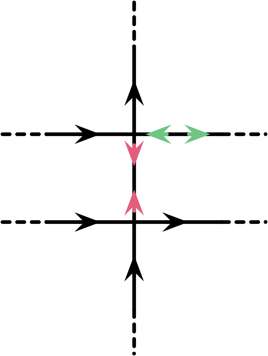
b

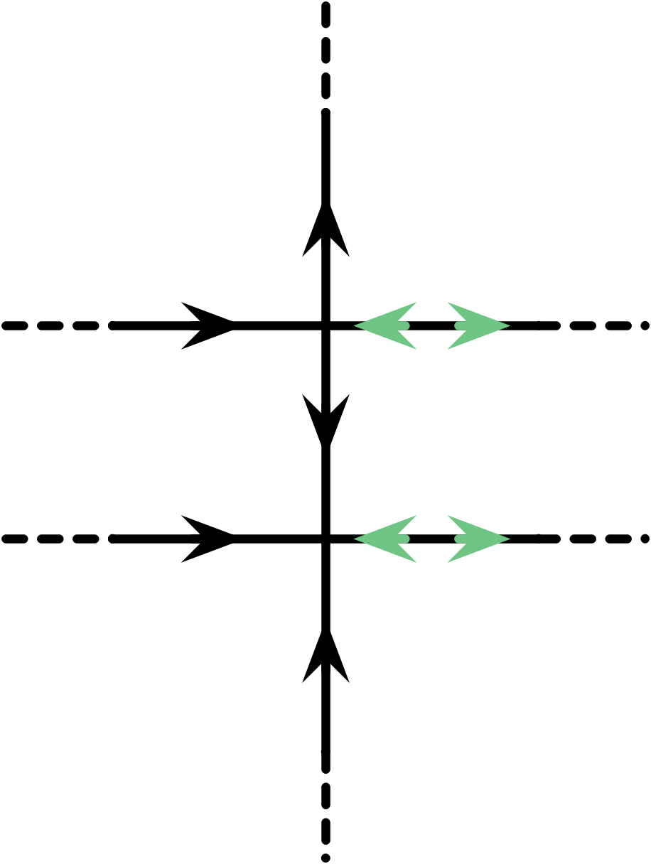
c

Figure 7: Examples of the states in the directed-loop algorithm.

Notation.

For a 4-regular graph, denote the set of even orientations by $\Omega_{0}$ and the set of near-even orientations by $\Omega_{2}$. The state space of $\mathcal{MC}$ is $\Omega=\Omega_{0}\cup\Omega_{2}$. Let $\mathcal{Z}(S)$ be the weighted sum of states in the set $S$.

Proof of Theorem 4.1.

We will show (later) that $\mathcal{MC}$ is irreducible and aperiodic, and it satisfies the detailed balance condition under the Gibbs distribution. By the theory of Markov chains, we have an almost uniform sampler of $\Omega_{0}\cup\Omega_{2}$. This sampler is efficient if $\mathcal{MC}$ is rapidly mixing. In this proof we show that for a 4-regular graph, if all constraint functions used in an instance belong to $\mathcal{F}_{\leq^{2}}\bigcap\mathcal{A}_{\leq}\bigcap\mathcal{B}_{\leq}\bigcap\mathcal{C}_{\leq}$, then

1. the $\mathcal{MC}$ is rapidly mixing via a conductance argument [JS89, DFK91, Sin92, Jer03];

2. even orientations take a non-negligible proportion in the state space;

3. there exists a self-reduction (to reduce the computation of the partition function of a graph to that of a “smaller” graph) [JVV86].

We remark that all three parts (1)(2)(3) depend on the idea of quantum decomposition and the closure properties shown in Section 3.

According to Lemma 4.5, when $(a,b,c,d)\in\mathcal{F}_{\leq^{2}}$, the conductance of this $\mathcal{MC}$ is polynomially bounded if $\frac{\mathcal{Z}(\Omega_{2})}{\mathcal{Z}(\Omega_{0})}$ is polynomially bounded. According to Corollary 4.3, when $(a,b,c,d)\in\mathcal{A}_{\leq}\bigcap\mathcal{B}_{\leq}\bigcap\mathcal{C}_{\leq}$, $\frac{\mathcal{Z}(\Omega_{2})}{\mathcal{Z}(\Omega_{0})}$ is polynomially bounded, which proves part (2) above. Combining Lemma 4.5 and Corollary 4.3, we can also conclude part (1). As a consequence of (1) and (2), we are able to efficiently sample valid eight-vertex configurations according to the Gibbs measure on $\Omega_{0}$ (almost uniformly), and in the following algorithm we only work with states in $\Omega_{0}$, the set of even orientations.

Before we state the algorithm, we need to extend the type of vertices a graph can have in the eight-vertex model. Previously, a graph can only have degree 4 vertices, on each of which a constraint function satisfies the even orientation rule and arrow reversal symmetry. Now, a graph can also have degree 2 vertices, on each of which the constraint function satisfies the “1-in-1-out” rule and both valid local configurations have weight $1$. Both Lemma 4.5 and Corollary 4.3 still hold with this extension, because such a degree 2 vertex and its two incident edges just work together as a single edge.

We design the following algorithm to approximately compute the partition function $Z(G)$ via sampling with the directed-loop algorithm $\mathcal{MC}$. As we have argued in Section 3, the partition function of the eight-vertex models can be viewed as the weighted sum over a set of dacp’s. Since every constraint function belongs to $\overline{\mathcal{F}_{>}}$, by Lemma 3.7 for each vertex we can choose a nonnegative weight function $w$ on signed pairings at $v$. For a vertex $v\in V$, the ratios among different signed pairings $\{\raisebox{-1.20007pt}{\includegraphics[height=8.39996pt,width=8.39996pt,keepaspectratio]{sub_1}},\raisebox{-1.20007pt}{\includegraphics[height=8.39996pt,width=8.39996pt,keepaspectratio]{sub_2}},\raisebox{-1.20007pt}{\includegraphics[height=8.39996pt,width=8.39996pt,keepaspectratio]{sub_3}}\}\times\{+,-\}$ in weighted dacp’s can be uniquely determined by the ratios among different orientations (represented by $a$, $b$, $c$, and $d$) at $v$. For example, if we express $Z(G)$ as $2aA+2bB+2cC+2dD$ according to the local orientation configuration at $v$, as in the proof of Corollary 3.8, we see that indeed $2w(\raisebox{-1.20007pt}{\includegraphics[height=8.39996pt,width=8.39996pt,keepaspectratio]{sub_1}}_{-})(A+D)$ is the weight for finding the signed pairing $\raisebox{-1.20007pt}{\includegraphics[height=8.39996pt,width=8.39996pt,keepaspectratio]{sub_1}}_{-}$ at $v$. As long as the partition function is not zero (this can be easily tested in polynomial time), there is a signed pairing $\boldsymbol{\varrho}$ showing up at $v$ with probability at least $\frac{1}{6}$ among all six signed pairings. Moreover, according to Corollary 3.8, one of the pairings in $\{\raisebox{-1.20007pt}{\includegraphics[height=8.39996pt,width=8.39996pt,keepaspectratio]{sub_1}}_{+},\raisebox{-1.20007pt}{\includegraphics[height=8.39996pt,width=8.39996pt,keepaspectratio]{sub_2}}_{+},\raisebox{-1.20007pt}{\includegraphics[height=8.39996pt,width=8.39996pt,keepaspectratio]{sub_3}}_{+}\}$ shows up at $v$ with probability at least $\frac{1}{6}$. Therefore, running $\mathcal{MC}$ on $G$, we can approximate, with a sufficient $1/{\rm poly}(n)$ precision, the probability of having $\boldsymbol{\varrho}\in\{\raisebox{-1.20007pt}{\includegraphics[height=8.39996pt,width=8.39996pt,keepaspectratio]{sub_1}}_{+},\raisebox{-1.20007pt}{\includegraphics[height=8.39996pt,width=8.39996pt,keepaspectratio]{sub_2}}_{+},\raisebox{-1.20007pt}{\includegraphics[height=8.39996pt,width=8.39996pt,keepaspectratio]{sub_3}}_{+}\}$ at $v$, denoted by $\Pr_{v}(\boldsymbol{\varrho})$. Denote by $G_{v,\boldsymbol{\varrho}}$ the graph with $v$ being split into $v_{1}$ and $v_{2}$ and the edges reconnected according to $\boldsymbol{\varrho}$. Recall that the degree 2 vertices $v_{1}$ and $v_{2}$ must satisfy the “1-in-1-out” rule in any valid configuration. Write the partition function of $G_{v,\boldsymbol{\varrho}}$ as $Z(G_{v,\boldsymbol{\varrho}})$, we have $\Pr_{v}(\boldsymbol{\varrho})=w(\boldsymbol{\varrho})Z(G_{v,\boldsymbol{\varrho}})/Z(G)$ which means $Z(G)=w(\boldsymbol{\varrho})Z(G_{v,\boldsymbol{\varrho}})/\Pr_{v}(\boldsymbol{\varrho})$. To approximate $Z(G)$ it suffices to approximate $Z(G_{v,\boldsymbol{\varrho}})$, which can be done by running $\mathcal{MC}$ on $G_{v,\boldsymbol{\varrho}}$ and recursing. Repeating this process for $|V|$ steps we decompose the graph $G$ into the base case, a set of disjoint cycles. The partition function of this cycle graph is just $2^{C}$ where $C$ is the number of cycles. By this self-reduction, the partition function $Z(G)$ can be approximated. ∎

Proof of Theorem 4.2.

The proof is similar to that of Theorem 4.1, with the help of Corollary 4.4 and Corollary 3.9, two corollaries of the closure property Theorem 3.3 which holds on planar graphs.

Given a plane graph $G$ with a constraint function on every vertex from $\mathcal{F}_{\leq^{2}}\bigcap\mathcal{A}_{\leq}\bigcap\mathcal{B}_{\leq}\bigcap\mathcal{C}_{\geq}$, we can still efficiently sample even orientations according to the Gibbs measure. However, in order to do self-reduction, we have to prove something more.

To make our algorithm work, we need to extend the type of vertices in the eight-vertex model again. Previously in the proof of Theorem 4.1, a graph can have degree 4 vertices, on each of which the constraint function satisfies the even orientation rule and arrow reversal symmetry, and degree 2 vertices, on each of which the constraint function satisfies the “1-in-1-out” rule and both valid local configurations have weight $1$. Now, a graph can also have degree 2 vertices, on each of which the constraint function satisfies the “2-in/2-out” rule and both valid local configurations have weight $1$. One can check that Lemma 4.5 still holds even with this extension.

The self-reduction still processes one vertex $v$ at a time. As long as the partition function is not zero, there is a signed pairing $\boldsymbol{\varrho}$ showing up at $v$ with probability at least $\frac{1}{6}$ among all six signed pairings. Moreover, according to Corollary 3.9, one of the pairings $\{\raisebox{-1.20007pt}{\includegraphics[height=8.39996pt,width=8.39996pt,keepaspectratio]{sub_1}}_{+},\raisebox{-1.20007pt}{\includegraphics[height=8.39996pt,width=8.39996pt,keepaspectratio]{sub_2}}_{+},\raisebox{-1.20007pt}{\includegraphics[height=8.39996pt,width=8.39996pt,keepaspectratio]{sub_3}}_{-}\}$ shows up at $v$ with probability at least $\frac{1}{6}$. If $\boldsymbol{\varrho}$ is $\raisebox{-1.20007pt}{\includegraphics[height=8.39996pt,width=8.39996pt,keepaspectratio]{sub_1}}_{+}$ or $\raisebox{-1.20007pt}{\includegraphics[height=8.39996pt,width=8.39996pt,keepaspectratio]{sub_2}}_{+}$, let $G_{v,\boldsymbol{\varrho}}$ be the graph with $v$ being split into $v_{1}$ and $v_{2}$ and the edges reconnected according to $\boldsymbol{\varrho}$. The degree 2 vertices $v_{1}$ and $v_{2}$ must satisfy the “1-in-1-out” rule in any valid configuration, just as in the proof of Theorem 4.1.

If $\boldsymbol{\varrho}$ is $\raisebox{-1.20007pt}{\includegraphics[height=8.39996pt,width=8.39996pt,keepaspectratio]{sub_3}}_{-}$, let $G_{v,\raisebox{-1.20007pt}{\includegraphics[height=8.39996pt,width=8.39996pt,keepaspectratio]{sub_3}}_{-}}$ be the graph with $v$ being split into $v_{1}$ and $v_{2}$ and the edges reconnected according to $\raisebox{-1.20007pt}{\includegraphics[height=8.39996pt,width=8.39996pt,keepaspectratio]{sub_3}}_{-}$. This time, the degree 2 vertices $v_{1}$ and $v_{2}$ must satisfy the “2-in/2-out” rule in any valid configuration. Observe that Theorem 3.3 holds for $G_{v,\raisebox{-1.20007pt}{\includegraphics[height=8.39996pt,width=8.39996pt,keepaspectratio]{sub_3}}_{-}}$ if and only if it holds for $G^{\prime}_{v,\raisebox{-1.20007pt}{\includegraphics[height=8.39996pt,width=8.39996pt,keepaspectratio]{sub_3}}_{-}}$, which is obtained from $G$ by replacing $v$ by a virtual vertex $v^{\prime}$ with parameter setting $(a,b,c,d)=(0,0,1,1)$ (this is equivalent to choosing $w(\raisebox{-1.20007pt}{\includegraphics[height=8.39996pt,width=8.39996pt,keepaspectratio]{sub_3}}_{-})=1$ and $w$ being 0 on the other five signed pairings, for a nonnegative $w$ at $v^{\prime}$). Since $(0,0,1,1)\in\mathcal{A}_{\leq}\bigcap\mathcal{B}_{\leq}\bigcap\mathcal{C}_{\geq}\bigcap\overline{\mathcal{F}_{>}}$, Theorem 3.3 and consequently Corollary 4.4 still hold for $G^{\prime}_{v,\raisebox{-1.20007pt}{\includegraphics[height=8.39996pt,width=8.39996pt,keepaspectratio]{sub_3}}_{-}}$ thus also for $G_{v,\raisebox{-1.20007pt}{\includegraphics[height=8.39996pt,width=8.39996pt,keepaspectratio]{sub_3}}_{-}}$. (Note that this $G^{\prime}_{v,\raisebox{-1.20007pt}{\includegraphics[height=8.39996pt,width=8.39996pt,keepaspectratio]{sub_3}}_{-}}$ is not involved algorithmically in subsequent steps; its only purpose is to show that Theorem 3.3 holds for $G_{v,\raisebox{-1.20007pt}{\includegraphics[height=8.39996pt,width=8.39996pt,keepaspectratio]{sub_3}}_{-}}$, on which the algorithm continues.)

The subsequent steps in the self-reduction step for $v$ are the same as in the proof of Theorem 4.1. The base case is a decomposition of $G$ into a set of disjoint cycles with an even number of degree 2 vertices that satisfy the “2-in/2-out” rule. This is proved by using the Jordan Curve Theorem: The graph is initially planar. Any step replacing $v$ with $v_{1}$ and $v_{2}$ for $\raisebox{-1.20007pt}{\includegraphics[height=8.39996pt,width=8.39996pt,keepaspectratio]{sub_1}}_{+}$ or $\raisebox{-1.20007pt}{\includegraphics[height=8.39996pt,width=8.39996pt,keepaspectratio]{sub_2}}_{+}$ in $G_{v,\boldsymbol{\varrho}}$ does not create any non-planar crossings nor vertices satisfying the “2-in/2-out” rule. Only the third type of steps replacing $v$ with $v_{1}$ and $v_{2}$ for $\raisebox{-1.20007pt}{\includegraphics[height=8.39996pt,width=8.39996pt,keepaspectratio]{sub_3}}_{-}$ in $G_{v,\raisebox{-1.20007pt}{\includegraphics[height=8.39996pt,width=8.39996pt,keepaspectratio]{sub_3}}_{-}}$ create a non-planar crossing and also a vertex satisfying the “2-in/2-out” rule at each crossing locally at each branch of the crossing. Thus at the end we are left with a set of disjoint cycles where along each cycle degree 2 vertices satisfying the “2-in/2-out” rule are in 1-1 correspondence with non-planar crossings. By the Jordan Curve Theorem this number is even, for every cycle. The partition function of this cycle graph is just $2^{C}$ where $C$ is the number of cycles. Again, the partition function $Z(G)$ can be approximated. ∎

Corollary 4.3.

Given a 4-regular graph $G=(V,E)$, if the constraint function on every vertex is from $\mathcal{A}_{\leq}\bigcap\mathcal{B}_{\leq}\bigcap\mathcal{C}_{\leq}$, then $\frac{\mathcal{Z}(\Omega_{2})}{\mathcal{Z}(\Omega_{0})}\leq\binom{|E|}{2}$.

Proof.

a A near-even orientation with defects at $e$ and $e^{\prime}$.

b A 4-ary construction by cutting open $e$ and $e^{\prime}$.

Figure 8:

For each near-even orientation, there are exactly two defective edges. Let $\Omega_{2}^{\{e,e^{\prime}\}}\subseteq\Omega_{2}$ be the set of near-even orientations in which $e,e^{\prime}$ are these two defective edges. We have $\frac{\mathcal{Z}(\Omega_{2})}{\mathcal{Z}(\Omega_{0})}=\sum_{\{e,e^{\prime}\}\ \in\ {E\choose 2}}\frac{\mathcal{Z}(\Omega_{2}^{\{e,e^{\prime}\}})}{\mathcal{Z}(\Omega_{0})}$.

For any $\tau\in\Omega_{2}$, each of $e$ and $e^{\prime}$ may have both half-edges coming in or going out, with 4 possibilities. An example is in Figure 8a where both $e$ and $e^{\prime}$ have their half-edges going out. If we “cut open” $e$ and $e^{\prime}$ as shown in Figure 8b, we get a 4-ary construction $\Gamma$ using degree 4 vertices with constraint functions in $\mathcal{A}_{\leq}\bigcap\mathcal{B}_{\leq}\bigcap\mathcal{C}_{\leq}$. Denote the constraint function of $\Gamma$ by $(a^{\prime},b^{\prime},c^{\prime},d^{\prime})$, with the input order being counter-clockwise starting from the upper-left edge. For this 4-ary construction $\Gamma$ we observe that: the set of near-even orientations in $\Omega_{2}^{\{e,e^{\prime}\}}$ contributes a total weight $(a^{\prime}+a^{\prime}+d^{\prime}+d^{\prime})$, i.e. $\mathcal{Z}(\Omega_{2}^{\{e,e^{\prime}\}})=2(a^{\prime}+d^{\prime})$; the set of even orientations in $\Omega_{0}$ has a total weight $\mathcal{Z}(\Omega_{0})=2(b^{\prime}+c^{\prime})$. By Theorem 3.2 we know that for the 4-ary construction $\Gamma$, $a^{\prime}+d^{\prime}\leq b^{\prime}+c^{\prime}$. Therefore, $\frac{\mathcal{Z}(\Omega_{2}^{\{e,e^{\prime}\}})}{\mathcal{Z}(\Omega_{0})}\leq 1$. In total, $\frac{\mathcal{Z}(\Omega_{2})}{\mathcal{Z}(\Omega_{0})}\leq\binom{|E|}{2}$. ∎

Corollary 4.4.

Given a 4-regular plane graph $G=(V,E)$, if the constraint function on every vertex is from $\mathcal{A}_{\leq}\bigcap\mathcal{B}_{\leq}\bigcap\mathcal{C}_{\geq}\bigcap\overline{\mathcal{F}_{>}}$, then $\frac{\mathcal{Z}(\Omega_{2})}{\mathcal{Z}(\Omega_{0})}\leq\binom{|E|}{2}$.

Proof.

For any 4-regular plane graph $G=(V,E)$, if we cut the two defective edges of $\tau\in\Omega_{2}$, we obtain a planar $\Gamma$ with 4 dangling edges using constraint functions from $\mathcal{A}_{\leq}\bigcap\mathcal{B}_{\leq}\bigcap\mathcal{C}_{\geq}\bigcap\overline{\mathcal{F}_{>}}$. We name $e_{1}$ and $e_{2}$ the two dangling edges cut from one edge in $G$, and $e_{3}$ and $e_{4}$ cut from the other. Both $e_{1}$ and $e_{2}$ now reside in a single face of $\Gamma$, and so do $e_{3}$ and $e_{4}$. We can modify the proof of Theorem 3.3 to establish that for $\Gamma$, we still have $a^{\prime}+d^{\prime}\leq b^{\prime}+c^{\prime}$. ∎

Although $\mathcal{MC}$ runs on the even orientations and near-even orientations of a 4-regular graph $G$, it is formally defined and analyzed using the edge-vertex incidence graph $G^{\prime}$ of $G$ introduced in Section 2.

Let $G^{\prime}=(V,U,E)$ be the edge-vertex incidence graph of $G$, an instance of $Z(a,b,c,d)$. Each vertex in $V$ is assigned $(\neq_{2})$; each vertex $u\in U$ is assigned a constraint function $f_{u}\in\mathcal{F}_{\leq^{2}}$. An assignment $\sigma$ assigns a value in $\{0,1\}$ to each edge $e\in E$. The state space of $\mathcal{MC}$ is $\Omega=\Omega_{0}\cup\Omega_{2}$, which consists of “perfect” or “near-perfect” assignments to $E$, defined as follows: all assignments satisfy the “two-0-two-1/four-0/four-1” rule at every vertex $u\in U$ of degree 4; all assignments satisfy the “one-0-one-1” at every $v\in V$ with possibly exactly two exceptions. Assignments in $\Omega_{0}$ have no exceptions, and are “perfect” (corresponding to the even orientations in $G$). Assignments in $\Omega_{2}$ have exactly two exceptions, and are “near-perfect” (corresponding to the near-even orientations in $G$). Thus any $\sigma\in\Omega_{0}$ sastifies all $(\neq_{2})$ on $V$, and any $\sigma\in\Omega_{2}$ sastifies all $(\neq_{2})$ on $V-\{v^{\prime},v^{\prime\prime}\}$ for some two vertices $v^{\prime},v^{\prime\prime}\in V$ where it satisfies $(=_{2})$ (which outputs 1 on inputs 00, 11 and outputs 0 on 01, 10). For any assignment $\sigma\in\Omega$ and any subset $S\subseteq\Omega$, define the weight function $\mathcal{W}$ by $\mathcal{W}(\sigma)=\prod_{u\in U}f_{u}(\sigma|_{E(u)})$ and $\mathcal{Z}(S)=\sum_{\sigma\in S}\mathcal{W}(\sigma)$. Then the Gibbs measure for $\Omega$ is defined by $\pi(\sigma)=\frac{\mathcal{W}(\sigma)}{\mathcal{Z}(\Omega)}$, assuming $\mathcal{Z}(\Omega)>0$.

Transitions in $\mathcal{MC}$ are comprised of three types of moves. Suppose $\sigma\in\Omega_{0}$. An $\Omega_{0}$-to-$\Omega_{2}$ move from $\sigma$ takes a degree 4 vertex $u\in U$ and two incident edges $e^{\prime}=(v^{\prime},u),e^{\prime\prime}=(v^{\prime\prime},u)\in V\times U$, and changes it to $\sigma_{2}\in\Omega_{2}$ which flips both $\sigma(e^{\prime})$ and $\sigma(e^{\prime\prime})$. The effect is that at $v^{\prime}$ and $v^{\prime\prime}$, $\sigma_{2}$ satisfies $(=_{2})$ instead of $(\neq_{2})$. An $\Omega_{2}$-to-$\Omega_{0}$ move is the opposite. An $\Omega_{2}$-to-$\Omega_{2}$ move is, intuitively, to shift one $(=_{2})$ from one vertex $v^{\prime}\in V$ to another $v^{*}\in V$, where for some $u\in U$, $v^{\prime}$ and $v^{*}$ are both incident to $u$ and the “two-0-two-1/four-0/four-1” rule at $u$ is preserved. Formally, let $\sigma\in\Omega_{2}$ be a near-perfect assignment with $v^{\prime},v^{\prime\prime}\in V$ being the two exceptional vertices (i.e., $\sigma$ satisfies $(=_{2})$ at $v^{\prime}$ and $v^{\prime\prime}$). Let $v^{*}\in V-\{v^{\prime},v^{\prime\prime}\}$ be such that for some $u\in U$, both $e^{\prime}=(v^{\prime},u),e^{*}=(v^{*},u)\in E$. Then an $\Omega_{2}$-to-$\Omega_{2}$ move changes $\sigma$ to $\sigma^{*}$ by flipping both $\sigma(e^{\prime})$ and $\sigma(e^{*})$. The effect is that $\sigma^{*}$ satisfies $(\neq_{2})$ at $v^{\prime}$ and $(=_{2})$ at $v^{*}$. Note that $\sigma^{*}$ continues to satisfy $(=_{2})$ at $v^{\prime\prime}$.

The above describes a symmetric binary relation neighbor ($\sim$) on $\Omega$. No two states in $\Omega_{0}$ are neighbors. Set $n=|U|$. The number of neighbors of a $\Omega_{0}$-state is at most $6n$ (by first picking a vertex and then picking a pair of edges incident to this vertex) and the number of neighbors of a $\Omega_{2}$-state is at most a constant. The transition probabilities $P(\cdot,\cdot)$ of $\mathcal{MC}$ are Metropolis moves between neighboring states:

$$P(\sigma_{1},\sigma_{2})=\left\{\begin{array}[]{ll}\frac{1}{12n}\min\left(1,\frac{\pi(\sigma_{2})}{\pi(\sigma_{1})}\right)&\text{if }\sigma_{2}\sim\sigma_{1};\\ 1-\frac{1}{12n}\sum_{\sigma^{\prime}\sim\sigma_{1}}\min\left(1,\frac{\pi(\sigma^{\prime})}{\pi(\sigma_{1})}\right)&\text{if }\sigma_{1}=\sigma_{2};\\ 0&\text{otherwise.}\end{array}\right.$$

$\mathcal{MC}$ is aperiodic due to the “lazy” movement; one can verify that $\mathcal{MC}$ is irreducible by creating, shifting, and merging two $(=_{2})$’s; as the transitions are Metropolis moves, detailed balance conditions are satisfied with regard to $\pi$. By results from [JS89, Sin92], such a Markov chain is rapidly mixing if there is a flow whose congestion can be bounded by a polynomial in $n$.

Lemma 4.5.

Assume $\mathcal{Z}(\Omega_{0})>0$. Given $f_{u}\in\mathcal{F}_{\leq^{2}}$ for every vertex $u\in U$, there is a flow on $\Omega$ with congestion at most $O\left(n^{2}\left(\frac{\mathcal{Z}(\Omega)}{\mathcal{Z}(\Omega_{0})}\right)^{2}\right)$, using paths of length $O(n)$.

Proof.

The idea is to design a flow $\mathfrak{F}:\mathcal{P}\rightarrow\mathbb{R}^{+}$ from $\Omega_{2}$ to $\Omega_{0}$ which satisfies

$$\sum_{p\in\mathcal{P}_{\sigma_{2}\sigma_{0}}}\mathfrak{F}(p)=\pi(\sigma_{2})\pi(\sigma_{0})\text{, \; for all }\sigma_{2}\in\Omega_{2},\sigma_{0}\in\Omega_{0},$$

where $\mathcal{P}_{\sigma_{2}\sigma_{0}}$ is defined to be a set of simple directed paths from $\sigma_{2}$ to $\sigma_{0}$ in $\mathcal{MC}$ and $\mathcal{P}=\bigcup_{\sigma_{2}\in\Omega_{2},\sigma_{0}\in\Omega_{0}}\mathcal{P}_{\sigma_{2}\sigma_{0}}$. Once the congestion of $\mathfrak{F}$ from $\Omega_{2}$ to $\Omega_{0}$ is polynomially bounded, so is the flow from $\Omega_{0}$ to $\Omega_{2}$ by symmetric construction. Moreover, there is a flow from $\Omega_{2}$ to $\Omega_{2}$ (or from $\Omega_{0}$ to $\Omega_{0}$) whose congestion can also be polynomially bounded by randomly picking an intermediate state in $\Omega_{0}$ (or $\Omega_{2}$, respectively). Thus we have a flow on $\Omega$ with polynomially bounded congestion. This technique has been used in [JSV04, McQ13]. In the following we show that the congestion of $\mathfrak{F}$ from $\Omega_{2}$ to $\Omega_{0}$ is bounded by $O(n^{2})\frac{\mathcal{Z}(\Omega_{2})}{\mathcal{Z}(\Omega_{0})}$. Then the bound in the lemma for a flow on $\Omega$ follows.

To describe the flow $\mathfrak{F}$, we first specify the sets of paths that are going to take the flow. In line with the definition of $\Omega_{0}$ and $\Omega_{2}$, we define $\Omega_{4}$ to be the set of assignments where there are exactly four violations of $(\neq_{2})$ in $V$. Let $\Omega^{\prime}=\Omega_{0}\cup\Omega_{2}\cup\Omega_{4}$. For $\sigma,\sigma^{\prime}\in\Omega^{\prime}$, let $\sigma\oplus\sigma^{\prime}$ denote the symmetric difference (or bitwise XOR), where we view $\sigma$ and $\sigma^{\prime}$ as two bit strings in $\{0,1\}^{|E|}$. This is a 0-1 assignment to the edge set of the edge-vertex incidence graph $G^{\prime}=(V,U,E)$ of $G$. We also treat $\sigma\oplus\sigma^{\prime}$ as an edge subset of $E$ (corresponding to bit positions having bit 1, where $\sigma$ and $\sigma^{\prime}$ assign opposite values), and this defines an edge-induced subgraph of $G^{\prime}$, which we will just call it $\sigma\oplus\sigma^{\prime}$. Since at every $u\in U$ of degree 4, the “two-0-two-1/four-0/four-1” rule is satisfied by both $\sigma$ and $\sigma^{\prime}$, this edge-induced subgraph has even degree (0, 2, or 4) at every $u\in U$.

Let us introduce the set of atcp’s (annotated trail & circuit partitions) for the symmetric difference $\sigma\oplus\sigma^{\prime}$. It is similar to the notions of acp for 4-regular graphs and atcp for 4-ary constructions defined in Section 3. Let us assume $\sigma\in\Omega_{0}$ and $\sigma^{\prime}\in\Omega_{2}$, and the set of atcp’s for $\sigma\oplus\sigma^{\prime}$ in general cases when $\sigma,\sigma^{\prime}\in\Omega^{\prime}$ can be similarly defined. If $\sigma\in\Omega_{0}$ and $\sigma^{\prime}\in\Omega_{2}$, on the edge where $\sigma^{\prime}$ is defective (but $\sigma\in\Omega_{0}$ is not), $\sigma\oplus\sigma^{\prime}$ has a degree 1 vertex. First we assign a pairing (that groups four incident edges into two unordered pairs) at every vertex of degree 4 in $\sigma\oplus\sigma^{\prime}$. This partitions the edges of $\sigma\oplus\sigma^{\prime}$ into a set of edge-disjoint circuits and exactly one trail which ends in the two vertices in $V$ of degree 1. Then we affix a $\pm$ at every vertex $u\in U$ of degree 2 or degree 4 in $\sigma\oplus\sigma^{\prime}$ as follows: If $u\in U$ has degree 4 in $\sigma\oplus\sigma^{\prime}$ then $\sigma$ and $\sigma^{\prime}$ represent total reversal orientations of each other at $u$, and thus the pairing at $u$ has the same sign according to Table 1 for $\sigma$ and $\sigma^{\prime}$. We affix this sign at $u$. If $u\in U$ has degree 2 in $\sigma\oplus\sigma^{\prime}$, then $\sigma$ and $\sigma^{\prime}$ disagree on exactly two edges. On these two edges, if one assigns 01 the other assigns 10 (and vice versa), and if one assigns 00 the other assigns 11 (and vice versa). We affix $+$ at $u$ in the first case, and $-$ in the second case. One can check that for any atcp $\varphi$ of $\sigma\oplus\sigma^{\prime}$, one encounters an even number of $-$ along any circuit of $\varphi$.

Denote by $U_{4}\subseteq U$ the degree-4 vertices in $\sigma\oplus\sigma^{\prime}$. Then there are exactly $3^{|U_{4}|}$ atcp’s for $\sigma\oplus\sigma^{\prime}$. Note that an atcp of $\sigma\oplus\sigma^{\prime}$ is uniquely determined by a family of signed pairings on $U_{4}$. This is a 1-1 correspondence and we will identify the two sets. For any signed pairing in $\{\raisebox{-1.20007pt}{\includegraphics[height=8.39996pt,width=8.39996pt,keepaspectratio]{sub_1}},\raisebox{-1.20007pt}{\includegraphics[height=8.39996pt,width=8.39996pt,keepaspectratio]{sub_2}},\raisebox{-1.20007pt}{\includegraphics[height=8.39996pt,width=8.39996pt,keepaspectratio]{sub_3}}\}\times\{+,-\}$ on a vertex $u$ with constraint matrix $M(f_{u})=\left[\begin{smallmatrix}d&&&a\\ &b&c&\\ &c&b&\\ a&&&d\end{smallmatrix}\right]$, define the weight function $\mathfrak{w}$ for signed pairings as follows, $\left\{\begin{smallmatrix}a^{2}=\mathfrak{w}(\raisebox{-1.20007pt}{\includegraphics[height=12.0pt,width=12.0pt,keepaspectratio]{sub_1}}_{-})+\mathfrak{w}(\raisebox{-1.20007pt}{\includegraphics[height=12.0pt,width=12.0pt,keepaspectratio]{sub_2}}_{+})+\mathfrak{w}(\raisebox{-1.20007pt}{\includegraphics[height=12.0pt,width=12.0pt,keepaspectratio]{sub_3}}_{+})\\ b^{2}=\mathfrak{w}(\raisebox{-1.20007pt}{\includegraphics[height=12.0pt,width=12.0pt,keepaspectratio]{sub_1}}_{+})+\mathfrak{w}(\raisebox{-1.20007pt}{\includegraphics[height=12.0pt,width=12.0pt,keepaspectratio]{sub_2}}_{-})+\mathfrak{w}(\raisebox{-1.20007pt}{\includegraphics[height=12.0pt,width=12.0pt,keepaspectratio]{sub_3}}_{+})\\ c^{2}=\mathfrak{w}(\raisebox{-1.20007pt}{\includegraphics[height=12.0pt,width=12.0pt,keepaspectratio]{sub_1}}_{+})+\mathfrak{w}(\raisebox{-1.20007pt}{\includegraphics[height=12.0pt,width=12.0pt,keepaspectratio]{sub_2}}_{+})+\mathfrak{w}(\raisebox{-1.20007pt}{\includegraphics[height=12.0pt,width=12.0pt,keepaspectratio]{sub_3}}_{-})\\ d^{2}=\mathfrak{w}(\raisebox{-1.20007pt}{\includegraphics[height=12.0pt,width=12.0pt,keepaspectratio]{sub_1}}_{-})+\mathfrak{w}(\raisebox{-1.20007pt}{\includegraphics[height=12.0pt,width=12.0pt,keepaspectratio]{sub_2}}_{-})+\mathfrak{w}(\raisebox{-1.20007pt}{\includegraphics[height=12.0pt,width=12.0pt,keepaspectratio]{sub_3}}_{-})\\ \end{smallmatrix}\right.$. Note that $\mathfrak{w}$ has a nonnegative solution if and only if $f_{u}\in\mathcal{F}_{\leq^{2}}$ by a proof similar to that of Lemma 3.7. Let $\Phi_{\sigma\oplus\sigma^{\prime}}$ be the set of atcp’s for $\sigma\oplus\sigma^{\prime}$. For $\varphi\in\Phi_{\sigma\oplus\sigma^{\prime}}$, define

$$\mathfrak{W}(\sigma,\sigma^{\prime},\varphi):=\left(\prod_{u\in U\setminus U_{4}}f_{u}\left(\sigma|_{E(u)}\right)f_{u}\left(\sigma^{\prime}|_{E(u)}\right)\right)\left(\prod_{u\in U_{4}}\mathfrak{w}(\varphi(u))\right),$$

where $\varphi(u)$ is the signed pairing given by $\varphi$ at $u$. Then for all distinct $\sigma,\sigma^{\prime}\in\Omega^{\prime}$, we have

$$\sum_{\varphi\in\Phi_{\sigma\oplus\sigma^{\prime}}}\mathfrak{W}(\sigma,\sigma^{\prime},\varphi) =\sum_{\varphi\in\Phi_{\sigma\oplus\sigma^{\prime}}}\left(\prod_{u\in U\setminus U_{4}}f_{u}\left(\sigma|_{E(u)}\right)f_{u}\left(\sigma^{\prime}|_{E(u)}\right)\right)\left(\prod_{u\in U_{4}}\mathfrak{w}(\varphi(u))\right)$$

$$=\left(\prod_{u\in U\setminus U_{4}}f_{u}\left(\sigma|_{E(u)}\right)f_{u}\left(\sigma^{\prime}|_{E(u)}\right)\right)\left(\sum_{\varphi\in\Phi_{\sigma\oplus\sigma^{\prime}}}\prod_{u\in U_{4}}\mathfrak{w}(\varphi(u))\right)$$

$$=\left(\prod_{u\in U\setminus U_{4}}f_{u}\left(\sigma|_{E(u)}\right)f_{u}\left(\sigma^{\prime}|_{E(u)}\right)\right)\left(\prod_{u\in U_{4}}f_{u}\left(\sigma|_{E(u)}\right)f_{u}\left(\sigma^{\prime}|_{E(u)}\right)\right)$$

$$=\prod_{u\in U}f_{u}\left(\sigma|_{E(u)}\right)f_{u}\left(\sigma^{\prime}|_{E(u)}\right)$$

$$=\mathcal{W}(\sigma)\mathcal{W}(\sigma^{\prime}).$$

The equality from line 2 to line 3 is due to the following: when the degree (in the induced subgraph $\sigma\oplus\sigma^{\prime}$) of a vertex $u\in U$ is 4, $\sigma$ and $\sigma^{\prime}$ must take the same value at $u$, since one represents a total reversal of all arrows of another; thus $f_{u}\left(\sigma|_{E(u)}\right)f_{u}\left(\sigma^{\prime}|_{E(u)}\right)$ is in $\{a^{2},b^{2},c^{2},d^{2}\}$. Then

$$\prod_{u\in U_{4}}f_{u}\left(\sigma|_{E(u)}\right)f_{u}\left(\sigma^{\prime}|_{E(u)}\right)=\sum_{\varphi\in\Phi_{\sigma\oplus\sigma^{\prime}}}\prod_{u\in U_{4}}\mathfrak{w}(\varphi(u))$$

is obtained by using the sum expressions for $a^{2}$, $b^{2}$, $c^{2}$, and $d^{2}$ in terms of $\mathfrak{w}(\raisebox{-1.20007pt}{\includegraphics[height=8.39996pt,width=8.39996pt,keepaspectratio]{sub_1}}_{+})$, $\mathfrak{w}(\raisebox{-1.20007pt}{\includegraphics[height=8.39996pt,width=8.39996pt,keepaspectratio]{sub_1}}_{-})$, $\mathfrak{w}(\raisebox{-1.20007pt}{\includegraphics[height=8.39996pt,width=8.39996pt,keepaspectratio]{sub_2}}_{+})$, $\mathfrak{w}(\raisebox{-1.20007pt}{\includegraphics[height=8.39996pt,width=8.39996pt,keepaspectratio]{sub_2}}_{-})$, $\mathfrak{w}(\raisebox{-1.20007pt}{\includegraphics[height=8.39996pt,width=8.39996pt,keepaspectratio]{sub_3}}_{+})$, and $\mathfrak{w}(\raisebox{-1.20007pt}{\includegraphics[height=8.39996pt,width=8.39996pt,keepaspectratio]{sub_3}}_{-})$, and then expressing the product-of-sums as a sum-of-products.

Now we are ready to specify the “paths” which take nonzero flow from $\sigma_{2}\in\Omega_{2}$ to $\sigma_{0}\in\Omega_{0}$. In order to transit from $\sigma_{2}$ to $\sigma_{0}$, paths in $\mathcal{P}_{\sigma_{2}\sigma_{0}}$ go through states in $\Omega$ that gradually decrease the number of conflicting assignments along trails and circuits in $\sigma_{2}\oplus\sigma_{0}$. We first specify a total order on $E$, the set of edges of $G^{\prime}$. This induces a total order on circuits by lexicographic order. In the induced subgraph $\sigma_{2}\oplus\sigma_{0}$, exactly two vertices in $V$ have degree 1 (called endpoints) and all other vertices have degree 2 or degree 4. The set of paths in $\mathcal{P}_{\sigma_{2}\sigma_{0}}$ are designed to be in 1-to-1 correspondence with elements in $\Phi_{\sigma_{2}\oplus\sigma_{0}}$. Given any family of signed pairings $\varphi\in\Phi_{\sigma_{2}\oplus\sigma_{0}}$, we have a unique decomposition of the induced subgraph $\sigma_{2}\oplus\sigma_{0}$ as an edge disjoint union of one trail $[e_{1}](v_{1},e^{\prime}_{1},u_{1},e_{2},v_{2},e^{\prime}_{2},u_{2},\ldots,e_{k},v_{k})[e^{\prime}_{k}]$ (where $e_{1}$ and $e^{\prime}_{k}$ are not part of the trail), and zero or more edge disjoint circuits, which are ordered lexicographically. Here $v_{i}\in V$ and $u_{i}\in U$, and the two exceptional vertices are $v_{1}$ and $v_{k}$ where $\sigma_{2}$ satisfies $(=_{2})$. The unique path $p_{\varphi}$ first reverses all arrows along the trail, starting from the smaller of $e^{\prime}_{1}$ and $e_{k}$. If we assume, without loss of generality, $e^{\prime}_{1}$ is the smaller one, then $p_{\varphi}$ “pushes” the $(=_{2})$ from $v_{1}$, to $v_{2}$, then to $v_{3},\ldots,v_{k-1}$, and then “merge” at $v_{k}$, arriving at a configuration in $\Omega_{0}$. Next $p_{\varphi}$ reverses all arrows on each circuit in lexicographic order, and within each circuit $C$ it starts at the least edge $e$ (according to the edge order) and reverses all arrows on $C$ in a cyclic order starting in the direction indicated by $\sigma_{2}$ on $e$. (Technically it flips a pair of incident edges to vertices in $U$ in each step.) Such paths $p_{\varphi}$ are well-defined and are valid paths in $\mathcal{MC}$ since along any path every state is in $\Omega=\Omega_{0}\cup\Omega_{2}$ and every move is a valid transition defined in $\mathcal{MC}$. With regard to the flow distribution, the flow value put on $p_{\varphi}$ is $\frac{\mathfrak{W}(\sigma_{2},\sigma_{0},\varphi)}{\left(\mathcal{Z}(\Omega)\right)^{2}}$, making the following hold for all $\sigma_{2}\in\Omega_{2},\sigma_{0}\in\Omega_{0}$:

$$\sum_{p_{\varphi}\in\mathcal{P}_{\sigma_{2}\sigma_{0}}}\mathfrak{F}(p_{\varphi}) =\sum_{\varphi\in\Phi_{\sigma_{2}\oplus\sigma_{0}}}\frac{\mathfrak{W}(\sigma_{2},\sigma_{0},\varphi)}{\left(\mathcal{Z}(\Omega)\right)^{2}}$$

$$=\frac{\mathcal{W}(\sigma_{2})\mathcal{W}(\sigma_{0})}{\left(\mathcal{Z}(\Omega)\right)^{2}}$$

$$=\pi(\sigma_{2})\pi(\sigma_{0}).$$

Note that in each path, no edge is flipped more than once, so the length is $O(n)$. For any transition $(\sigma^{\prime},\sigma^{\prime\prime})$ where $\sigma^{\prime}\neq\sigma^{\prime\prime}$, we have $P(\sigma^{\prime},\sigma^{\prime\prime})=\frac{1}{12n}\min\left(1,\frac{\pi(\sigma^{\prime\prime})}{\pi(\sigma^{\prime})}\right)=\Omega\left(\frac{1}{n}\right)$, as $\frac{\pi(\sigma^{\prime\prime})}{\pi(\sigma^{\prime})}$ is a constant. (This is a constant because we have restricted the constraint function $f_{u}$ to be from a fixed finite set $\mathcal{F}$.) Let $H_{\sigma^{\prime}}=\{\sigma_{2}\oplus\sigma_{0}\ |\ \sigma_{2}\in\Omega_{2},\sigma_{0}\in\Omega_{0},\exists\varphi\in\Phi_{\sigma_{2}\oplus\sigma_{0}}\text{ s.t. }\sigma^{\prime}\in p_{\varphi}\}$. The congestion of $\mathfrak{F}$ is

$$\max_{\text{transition }(\sigma^{\prime},\sigma^{\prime\prime})}\frac{1}{\pi(\sigma^{\prime})P(\sigma^{\prime},\sigma^{\prime\prime})}\sum_{\begin{subarray}{c}\sigma_{2}\in\Omega_{2}\\ \sigma_{0}\in\Omega_{0}\end{subarray}}\sum_{\begin{subarray}{c}p_{\varphi}\in\mathcal{P}_{\sigma_{2}\sigma_{0}}\\ p_{\varphi}\ni(\sigma^{\prime},\sigma^{\prime\prime})\end{subarray}}\frac{\mathfrak{W}(\sigma_{2},\sigma_{0},\varphi)}{\left(\mathcal{Z}(\Omega)\right)^{2}}$$

$$\leq \max_{\sigma^{\prime}\in\Omega}\frac{O(n)}{\mathcal{W}(\sigma^{\prime})\mathcal{Z}(\Omega)}\sum_{\begin{subarray}{c}\sigma_{2}\in\Omega_{2}\\ \sigma_{0}\in\Omega_{0}\end{subarray}}\sum_{\begin{subarray}{c}\varphi\in\Phi_{\sigma_{2}\oplus\sigma_{0}}\\ p_{\varphi}\ni\sigma^{\prime}\end{subarray}}\mathfrak{W}(\sigma_{2},\sigma_{0},\varphi)$$

$$\leq \max_{\sigma^{\prime}\in\Omega}\frac{O(n)}{\mathcal{W}(\sigma^{\prime})\mathcal{Z}(\Omega)}\sum_{\sigma_{2}\in\Omega_{2}}\sum_{\eta\in H_{\sigma^{\prime}}}\sum_{\varphi\in\Phi_{\eta}}\mathfrak{W}(\sigma_{2},\sigma_{2}\oplus\eta,\varphi)$$

$$= \max_{\sigma^{\prime}\in\Omega}\frac{O(n)}{\mathcal{W}(\sigma^{\prime})\mathcal{Z}(\Omega)}\sum_{\eta\in H_{\sigma^{\prime}}}\sum_{\varphi\in\Phi_{\eta}}\sum_{\sigma_{2}\in\widetilde{\Omega}_{2}}\mathfrak{W}(\sigma_{2},\sigma_{2}\oplus\eta,\varphi).$$

On the last line above we exchange the order of summations where $\widetilde{\Omega}_{2}$ is the subset of $\Omega_{2}$-states of the form $\sigma_{2}=\eta\oplus\sigma_{0}$, for some $\sigma_{0}\in\Omega_{0}$ such that $p_{\varphi}$ (which passes through $\sigma^{\prime}$) goes from $\sigma_{2}$ to $\sigma_{0}$. These are $\Omega_{2}$-states “compatible” with the symmetric difference $\eta$ and its atcp $\varphi$. The number of states in $\widetilde{\Omega}_{2}$ is bounded by the length of the longest path $O(n)$ because $\sigma^{\prime}$ is an intermediate state on a path. Fix any $\sigma^{\prime}\in\Omega$. For any $\sigma_{2}\in\Omega_{2}$, and $\eta\in H_{\sigma^{\prime}}$ consisting of exactly one connected component with two endpoints of degree 1 and all other vertices having even degree (and zero or more connected components of even degree vertices), observe that $\sigma^{\prime}\oplus\eta\in\Omega^{\prime}$. Indeed, if $\sigma^{\prime}\in\Omega_{0}$ then $\sigma^{\prime}\oplus\eta\in\Omega_{2}$; if $\sigma^{\prime}\in\Omega_{2}$ then depending on whether $\sigma^{\prime}$

1. is $\sigma_{2}$, or

2. appears in the process of reversing arrows on the trail with two endpoints, or

3. appears after reversing arrows on the trail with endpoints,

$\sigma^{\prime}\oplus\eta$ lies in $\Omega_{0}$, $\Omega_{2}$, or $\Omega_{4}$, respectively. For the edges not in $\eta$, $\sigma^{\prime}$ agrees with $\sigma_{2}$ and $\sigma_{2}\oplus\eta$ as the path $p_{\varphi}$ never “touches” them, and so does $\sigma^{\prime}\oplus\eta$. Recall that

$$\mathfrak{W}(\sigma_{2},\sigma_{2}\oplus\eta,\varphi)=\left(\prod_{u\in U\setminus U_{4}}f_{u}\left(\sigma_{2}|_{E(u)}\right)f_{u}\left((\sigma_{2}\oplus\eta)|_{E(u)}\right)\right)\left(\prod_{u\in U_{4}}\mathfrak{w}(\varphi(u))\right).$$

For every vertex $u\in U$ that is not in $\eta$, $f_{u}$ takes the same value in all $\sigma_{2}$, $\sigma_{2}\oplus\eta$, $\sigma^{\prime}$, and $\sigma^{\prime}\oplus\eta$. For every vertex $u\in U$ that is degree-2 in $\eta$, assuming $M(f_{u})=\left[\begin{smallmatrix}d&&&a\\ &b&c&\\ &c&b&\\ a&&&d\end{smallmatrix}\right]$, $f_{u}\left(\sigma_{2}|_{E(u)}\right)$ and $f_{u}\left((\sigma_{2}\oplus\eta)|_{E(u)}\right)$ take two different elements in $\{a,b,c,d\}$. Meanwhile, $f_{u}\left(\sigma^{\prime}|_{E(u)}\right)$ and $f_{u}\left(\sigma^{\prime}\oplus\eta|_{E(u)}\right)$ also take these two elements (possibly in the opposite order). For example, at the vertex $u$ shown in Figure 9, $f_{u}\left(\sigma_{2}|_{E(u)}\right)=a$ and $f_{u}\left(\sigma_{2}\oplus\eta|_{E(u)}\right)=c$. The two solid edges are in $\eta$ and assignments on the two dotted edges are shared by $\sigma_{2}$ and $\sigma_{2}\oplus\eta$, as well as $\sigma^{\prime}$ and $\sigma^{\prime}\oplus\eta$. On the path $p_{\varphi}$ from $\sigma_{2}$ to $\sigma_{2}\oplus\eta$ decided by $\varphi$: if $\sigma^{\prime}$ appears before reversing the two solid edges, then $\sigma^{\prime}$ agrees with $\sigma_{2}$ on them ($f_{u}\left(\sigma^{\prime}|_{E(u)}\right)=a$) and $\sigma^{\prime}\oplus\eta$ agrees with $\sigma_{2}\oplus\eta$ on them ($f_{u}\left(\sigma^{\prime}\oplus\eta|_{E(u)}\right)=c$); if $\sigma^{\prime}$ appears after reversing the two solid edges, then $\sigma^{\prime}$ agrees with $\sigma_{2}\oplus\eta$ on them ($f_{u}\left(\sigma^{\prime}|_{E(u)}\right)=c$) and $\sigma^{\prime}\oplus\eta$ agrees with $\sigma_{2}$ on them ($f_{u}\left(\sigma^{\prime}\oplus\eta|_{E(u)}\right)=a$). For every vertex $u\in U$ that is degree-4 in $\eta$, $\mathfrak{w}(\varphi(u))$ takes the same value in $\mathfrak{W}(\sigma_{2},\sigma_{2}\oplus\eta,\varphi)$ and $\mathfrak{W}(\sigma^{\prime},\sigma^{\prime}\oplus\eta,\varphi)$ as the weight only depends on $\varphi(u)$, the signed pairing at $u$.

a $\sigma_{2}$.

b $\sigma_{2}\oplus\eta$.

Figure 9:

By the above argument, we established that $\mathfrak{W}(\sigma_{2},\sigma_{2}\oplus\eta,\varphi)=\mathfrak{W}(\sigma^{\prime},\sigma^{\prime}\oplus\eta,\varphi)$. Therefore, the congestion of $\mathfrak{F}$ can be bounded by

$$\max_{\sigma^{\prime}\in\Omega}\frac{O(n)}{\mathcal{W}(\sigma^{\prime})\mathcal{Z}(\Omega)}\sum_{\eta\in H_{\sigma^{\prime}}}\sum_{\varphi\in\Phi_{\eta}}\sum_{\sigma_{2}\in\widetilde{\Omega}_{2}}\mathfrak{W}(\sigma^{\prime},\sigma^{\prime}\oplus\eta,\varphi)$$

$$\leq \max_{\sigma^{\prime}\in\Omega}\frac{O(n^{2})}{\mathcal{W}(\sigma^{\prime})\mathcal{Z}(\Omega)}\sum_{\eta\in H_{\sigma^{\prime}}}\sum_{\varphi\in\Phi_{\eta}}\mathfrak{W}(\sigma^{\prime},\sigma^{\prime}\oplus\eta,\varphi)$$

$$\leq \max_{\sigma^{\prime}\in\Omega}\frac{O(n^{2})}{\mathcal{W}(\sigma^{\prime})\mathcal{Z}(\Omega)}\sum_{\eta\in H_{\sigma^{\prime}}}\mathcal{W}(\sigma^{\prime})\mathcal{W}(\sigma^{\prime}\oplus\eta)$$

$$= \max_{\sigma^{\prime}\in\Omega}\frac{O(n^{2})}{\mathcal{Z}(\Omega)}\sum_{\eta\in H_{\sigma^{\prime}}}\mathcal{W}(\sigma^{\prime}\oplus\eta)$$

$$\leq \frac{O(n^{2})}{\mathcal{Z}(\Omega)}\sum_{\sigma\in\Omega^{\prime}}\mathcal{W}(\sigma)$$

$$= O(n^{2})\frac{\mathcal{Z}(\Omega^{\prime})}{\mathcal{Z}(\Omega)}.$$

By a standard argument as in [JS89, MW96, McQ13], $\frac{\mathcal{Z}(\Omega_{4})}{\mathcal{Z}(\Omega_{2})}\leq\frac{\mathcal{Z}(\Omega_{2})}{\mathcal{Z}(\Omega_{0})}$. Therefore, the congestion is bounded by $O(n^{2})\frac{\mathcal{Z}(\Omega_{2})}{\mathcal{Z}(\Omega_{0})}$. ∎

Remark 4.2.

Lemma 4.5 can be alternatively derived using the notion of “windability” [McQ13].

5 Hardness

Theorem 5.1.

If $(a,b,c,d)\in\mathcal{F}_{>}$, then $Z(a,b,c,d)$ does not have an FPRAS unless RP=NP.

Remark 5.1.

For any $(a,b,c,d)\in\mathcal{F}_{>}$, there are at least two nonzero numbers among $a$, $b$, $c$, and $d$. The case $d=0$ and $a,b,c>0$ was proved in  [CLL19]. The case $d=0$ and one of $a,b,c$ is zero can be proved by a reduction from computing the partition function of the anti-ferromagnetic Ising model on 3-regular graphs; we postpone this proof to an expanded version of this paper. In this section, we prove the theorem when $d>0$ and at least one of $a,b,c$ is positive.

Remark 5.2.

The construction in our proof for the cases when $a>b+c+d$, or $b>a+c+d$, or $c>a+b+d$, is in fact a bipartite graph. This means that approximating $Z(a,b,c,d)$ in those cases is NP-hard even for bipartite graphs.

Proof.

Let 3-MAX CUT denote the NP-hard problem of computing the cardinality of a maximum cut in a 3-regular graph [Yan78]. We reduce 3-MAX CUT to approximating $Z(a,b,c,d)$. We first prove the case when $a>b+c+d$, then adapt our proof to the case when $d>a+b+c$. Since the proof of NP-hardness for $Z(a,b,c,d)$ is for general (i.e., not necessarily planar) graphs, we can permute the parameters $a,b,c$. Thus the proof for $b>a+c+d$ and $c>a+b+d$ is symmetric to the first case.

Before proving the theorem we briefly state our idea. Denote an instance of 3-MAX CUT by $G=(V,E)$. Given $V_{+}\subseteq V$ and $V_{-}=V\setminus V_{+}$, an edge $\{u,v\}\in E$ is in the cut between $V_{+}$ and $V_{-}$ if and only if $(u\in V_{+},v\in V_{-})$ or $(u\in V_{-},v\in V_{+})$. The maximum cut problem favors the partition of $V$ into $V_{+}$ and $V_{-}$ so that there are as many edges in $V_{+}\times V_{-}$ as possible. We want to encode this local preference on each edge by a local fragment of a graph $G^{\prime}$ in terms of configurations in the eight-vertex model.

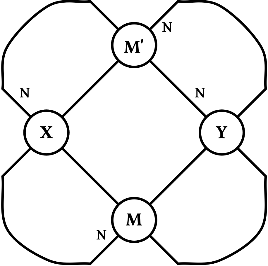
a

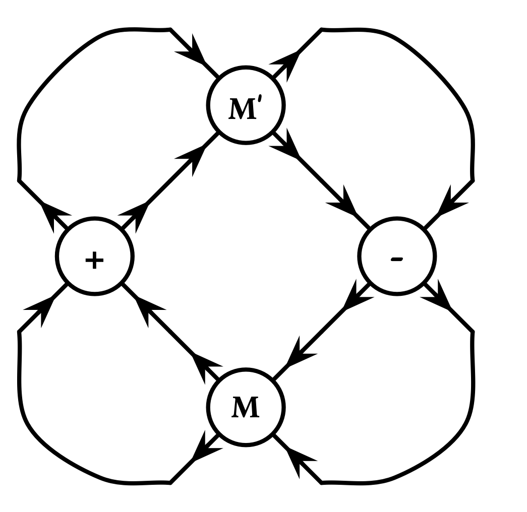
b

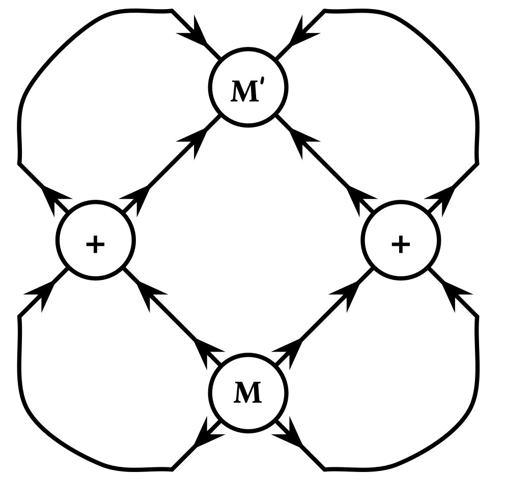
c

Figure 10: A four-way connection implementing a single edge in 3-MAX CUT.

Let us start with the case when $a>b+c+d$. Recall that we require $d>0$. First we show how to implement a toy example—a single edge $\{u,v\}$—by a construction in the eight-vertex model. Suppose there are four vertices $X,Y,M,M^{\prime}$ connected as in Figure 10a shows. The order of the 4 edges at each vertex is aligned to Figure 1 by a rotation so that the edge marked by “N” corresponds to the north edge in Figure 1. Let us impose the virtual constraint on $X$ and $Y$ so that the parameter setting on each of them is $\check{a}>\check{b}=\check{c}=\check{d}=0$. (We will show how to implement this virtual constraint in the sense of approximation later.) In other words, the four edges incident on $X$ can only be in two possible configurations, Figure 1-1 or Figure 1-2. The same is true for $Y$. We say $X$ (and similarly $Y$) is in state $+$ if its local configuration is in Figure 1-1 (with the “top” two edges going out and the “bottom” two edges coming in); it is in state $-$ if its local configuration is in Figure 1-2 (with the “top” two edges coming in and the “bottom” two edges going out). Hence there are a total of 4 valid configurations given the virtual constraints. When $(X,Y)$ is in state $(+,-)$ (or $(-,+)$), $M$ and $M^{\prime}$ have local configurations both being Figure 1-1 (or both being Figure 1-2), with weight $a$ (Figure 10b); when $(X,Y)$ is in state $(+,+)$ (or $(-,-)$), $M$ and $M^{\prime}$ have local configurations both being Figure 1-7 or Figure 1-8, with weight $d<a$ (Figure 10c). This models how two adjacent vertices interact in 3-MAX CUT. We will call the connection pattern described in Figure 10a between the set of 4 external edges incident to $X$ and the set of 4 external edges incident to $Y$ (each with two on “top” and two on “bottom”) a four-way connection.

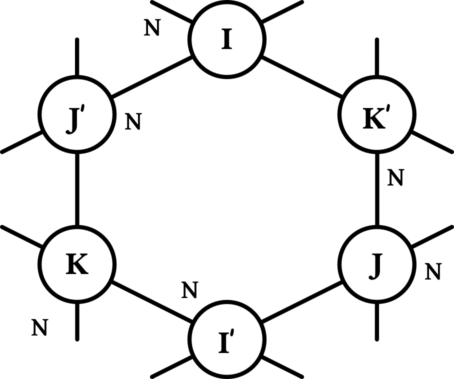
a

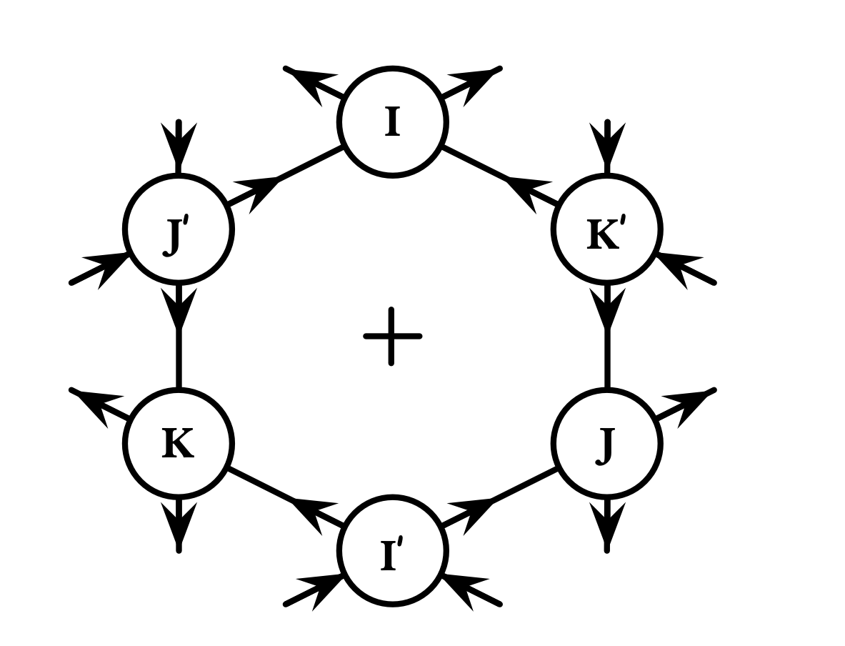
b

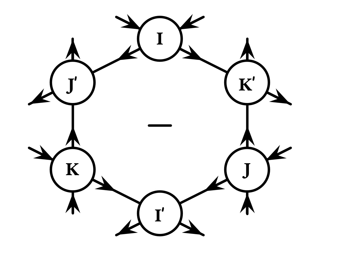
c

Figure 11: A locking device implementing a vertex of degree 3 in 3-MAX CUT.

To model a vertex of degree 3 in a 3-MAX CUT instance, we use the locking device in Figure 11a. Let us assume we have the virtual constraint that each of $I,I^{\prime},J,J^{\prime},K,K^{\prime}$ can only be in two local configurations, Figure 1-1 or Figure 1-2. In fact, each locking device has two states, one shown in Figure 11b with every node in configuration Figure 1-1 (called the $+$ state) and the other shown in Figure 11c with every node in configuration Figure 1-2 (called the $-$ state). If we think of the external edges incident to $I,J,K$ to serve as the “top” edges (with “N” aligned with the “N” at $X$ or $Y$ in Figure 10a), and the edges incident to $I^{\prime},J^{\prime},K^{\prime}$ as the “bottom” edges there, then we simulate the $\pm$ state of a degree 3 vertex as follows: (1) top edges are going out and bottom edges are coming in if the device is in $+$ state, and top edges are coming in and bottom edges are going out if the device is in $-$ state; and (2) the top edges on $I,J,K$ are going out or coming in at the same time.

Figure 12: A 4-ary construction that amplifies the maximum among $a,b,c,d$.

Next we show how to enforce the virtual constraint in Figure 11a that each vertex has two contrary configurations, in the sense of approximation. The idea is to implement an amplifier as a 4-ary construction with parameter $(\hat{a},\hat{b},\hat{c},\hat{d})$ such that $\hat{a}\gg\hat{b}+\hat{c}+\hat{d}$ using polynomially many vertices in the eight-vertex model. We obtain such an amplifier by an iteration of $\Gamma$ shown in Figure 12 (input edges of $B,C,D$ labeled similarly as for $A$ and those of $P,Q$ labeled similarly as for $O$). Starting with $(a,b,c,d)$ on every vertex in $\Gamma$ (where $a>b+c+d$), the parameter setting $(a^{\prime},b^{\prime},c^{\prime},d^{\prime})$ of $\Gamma$ is $\left\{\begin{smallmatrix}a^{\prime}=\Lambda(a,b,c,d)\\ b^{\prime}=\Lambda(b,c,d,a)\\ c^{\prime}=\Lambda(c,d,a,b)\\ d^{\prime}=\Lambda(d,a,b,c)\\ \end{smallmatrix}\right.$, where

$$\Lambda(\xi,x,y,z)=\xi^{7}+(3x^{4}+3y^{4}+3z^{4}+4x^{2}y^{2}+4x^{2}z^{2}+4y^{2}z^{2})\xi^{3}\\ +(2x^{4}y^{2}+2x^{4}z^{2}+2x^{2}y^{4}+2y^{4}z^{2}+2x^{2}z^{4}+2y^{2}z^{4}+30x^{2}y^{2}z^{2})\xi.$$ (5.1)

This construction uses $7$ vertices and is called a $1$-amplifier. We obtain $(a_{1},b_{1},c_{1},d_{1})=(a^{\prime},b^{\prime},c^{\prime},d^{\prime})$ which amplifies the relative weight of configurations in Figure 1-1 or Figure 1-2. If we plug in the amplifier $\Gamma$ into each vertex of $\Gamma$ itself (called a $2$-amplifier), we can obtain $(a_{2},b_{2},c_{2},d_{2})$ using $7^{2}$ vertices. Iteratively, we can construct a series of constraint functions with parameters $(a_{k},b_{k},c_{k},d_{k})\ (k\geq 1)$ such that $\left\{\begin{smallmatrix}a_{k+1}=\Lambda(a_{k},b_{k},c_{k},d_{k})\\ b_{k+1}=\Lambda(b_{k},c_{k},d_{k},a_{k})\\ c_{k+1}=\Lambda(c_{k},d_{k},a_{k},b_{k})\\ d_{k+1}=\Lambda(d_{k},a_{k},b_{k},c_{k})\\ \end{smallmatrix}\right.$, using $7^{k}$ vertices for each $k$ (called a $k$-amplifier). Lemma 5.2 shows that the asymptotic growth rate is exponential in the number of vertices used.

To reduce the problem 3-MAX CUT to approximating $Z(a,b,c,d)$, let $\kappa>\lambda\geq 1$ be two constants that will be fixed later. For each 3-MAX CUT instance $G=(V,E)$ with $|V|=n$ and $|E|=m$, we construct a graph $G^{\prime}$ where a device in Figure 11a is created for each $v\in V$, and a four-way connection is made for every $\{u,v\}\in E(G)$, on the external edges corresponding to $\{u,v\}$ as in Figure 10a. For each 4-way connection in Figure 10a, each of the nodes $M,M^{\prime}$ is replaced by a $(\lambda\log n)$-amplifier to boost the ratio of the configurations in Figure 1-1 or Figure 1-2 over other configurations. For each device in Figure 11a, each of the nodes $I,I^{\prime},J,J^{\prime},K,K^{\prime}$ is replaced by a $(\kappa\log n)$-amplifier to lock in the configurations Figure 11b or Figure 11c.

Next we argue that the maximum size $s$ of all cuts in $G$ can be recovered from an approximate solution to $Z(G^{\prime};a,b,c,d)$.

Given a cut $(V_{+},V_{-})$ of size $s$ in $G$, we show there is a valid configuration (at the granularity of nodes and edges shown in Figure 11a) of weight $\geq\left(a_{\kappa\log n}\right)^{6n}\left(a_{\lambda\log n}\right)^{2s}\left(d_{\lambda\log n}\right)^{2(m-s)}$. For every vertex $u\in V_{+}$ and every $v\in V_{-}$ we set the corresponding locking devices in the $+$ state (Figure 11b) and $-$ state (Figure 11c) respectively. Consequently, for each edge $\{u,v\}$, the two nodes $M$ and $M^{\prime}$ in the 4-way connection between the external edges from $u$ and $v$ (two from each) are both in Figure 1-1 or Figure 1-2 if $\{u,v\}$ is in the cut; they are both in Figure 1-7 or Figure 1-8 if $\{u,v\}$ is not in the cut. We have defined a valid configuration, and it has weight $\geq\prod_{v\in V}\left({a_{\kappa\log n}}\right)^{6}\prod_{e\in V_{+}\times V_{-}}\left(a_{\lambda\log n}\right)^{2}\prod_{e\not\in V_{+}\times V_{-}}\left(d_{\lambda\log n}\right)^{2}=\left(a_{\kappa\log n}\right)^{6n}\left(a_{\lambda\log n}\right)^{2s}\left(d_{\lambda\log n}\right)^{2(m-s)}$, where the exponent $6$ comes from the 6 nodes $I,I^{\prime},J,J^{\prime},K,K^{\prime}$ in each locking device and $2$ comes from the two nodes $M,M^{\prime}$ in each four-way connection.

We also show that the weighted sum of all configurations is $<\frac{1}{2}\left(a_{\kappa\log n}\right)^{6n}\left(a_{\lambda\log n}\right)^{2(s+1)}\left(d_{\lambda\log n}\right)^{2(m-(s+1))}$, where $s$ is the maximum size of cuts in $G$. First we bound $W_{\rm lock}$, the sum of weights for configurations where all nodes labeled $I,I^{\prime},J,J^{\prime},K,K^{\prime}$ are locked. It follows that

$$W_{\rm lock}\leq 2^{n}\left(a_{\kappa\log n}\right)^{6n}\sum_{i=0}^{s}\binom{m}{i}\left(a_{\lambda\log n}\right)^{2i}\left(d_{\lambda\log n}\right)^{2(m-i)}\leq 2^{n+m}\left(a_{\kappa\log n}\right)^{6n}\left(a_{\lambda\log n}\right)^{2s}\left(d_{\lambda\log n}\right)^{2(m-s)},$$

where each locking device has 2 possible states each with weight $\left(a_{\kappa\log n}\right)^{6}$, and given a particular $\pm$ assignment of $n$ devices, there can be at most $s$ four-way connections that are between a $+$ device and a $-$ device. Hence $W_{\rm lock}<\frac{1}{4}\left(a_{\kappa\log n}\right)^{6n}\left(a_{\lambda\log n}\right)^{2(s+1)}\left(d_{\lambda\log n}\right)^{2(m-(s+1))}$ when $\lambda\geq 1$ is large.

It remains to upper-bound the weighted sum of configurations where there is at least one device with some lock broken. This quantity is bounded by

$$8^{6n}\sum_{i=0}^{6n-1}\binom{6n}{i}\left(a_{\kappa\log n}\right)^{i}\left(b_{\kappa\log n}+c_{\kappa\log n}+d_{\kappa\log n}\right)^{(6n-i)}\left[2\left(a_{\lambda\log n}+b_{\lambda\log n}+c_{\lambda\log n}+d_{\lambda\log n}\right)\right]^{2m}$$

$$\leq\; 2^{24n+2m}\left(a_{\kappa\log n}\right)^{6n}\left(\frac{b_{\kappa\log n}+c_{\kappa\log n}+d_{\kappa\log n}}{a_{\kappa\log n}}\right)\left(a_{\lambda\log n}+b_{\lambda\log n}+c_{\lambda\log n}+d_{\lambda\log n}\right)^{2m}$$

$$\leq\; 2^{24n+6m}\left(a_{\kappa\log n}\right)^{6n}\left(\frac{b_{\kappa\log n}+c_{\kappa\log n}+d_{\kappa\log n}}{a_{\kappa\log n}}\right)\left(a_{\lambda\log n}\right)^{2m}$$

$$\leq\; 2^{24n+6m}\left[\Theta(1)\right]^{mn^{6\lambda}}\left(a_{\kappa\log n}\right)^{6n}\frac{1}{\beta^{n^{\kappa}}},$$

where we use the fact that $a_{\lambda\log n}\leq a^{64^{{\lambda\log n}}}=a^{n^{6\lambda}}$ because there are in total $64=2^{6}$ terms in (5.1) and $\beta>1$ by Lemma 5.2. This quantity is $<\frac{1}{4}\left(a_{\kappa\log n}\right)^{6n}$ when $\kappa>\lambda\geq 1$ is sufficiently large.

We have finished the proof for $a>b+c+d$. The case when $b>a+c+d$ or $c>a+b+d$ can be similarly proved. We now adapt our proof to the case when $d>a+b+c$. Since not all $a,b,c=0$ by our assumption, let us assume without loss of generality that $a>0$. The amplifier remains exactly the same thanks to its symmetry. For the locking device, we can still lock into two states (with the help of amplifiers on each node in the device): the $+$ state where $I,J,K$ are sources and $I^{\prime},J^{\prime},K^{\prime}$ are sinks; the $-$ state where $I,J,K$ are sinks and $I^{\prime},J^{\prime},K^{\prime}$ are sources. The only difference in the construction is the way that four-way connections are set up (Figure 13a). This time, a node marked with $I,J,K$ in one locking device need to be connected to a node marked with $I^{\prime},J^{\prime},K^{\prime}$ (instead of still $I,J,K$ as is the case when $a>b+c+d$) in another locking device to make sure locking devices in contrary states are favored (by setting $M$ and $M^{\prime}$ as sinks and sources).

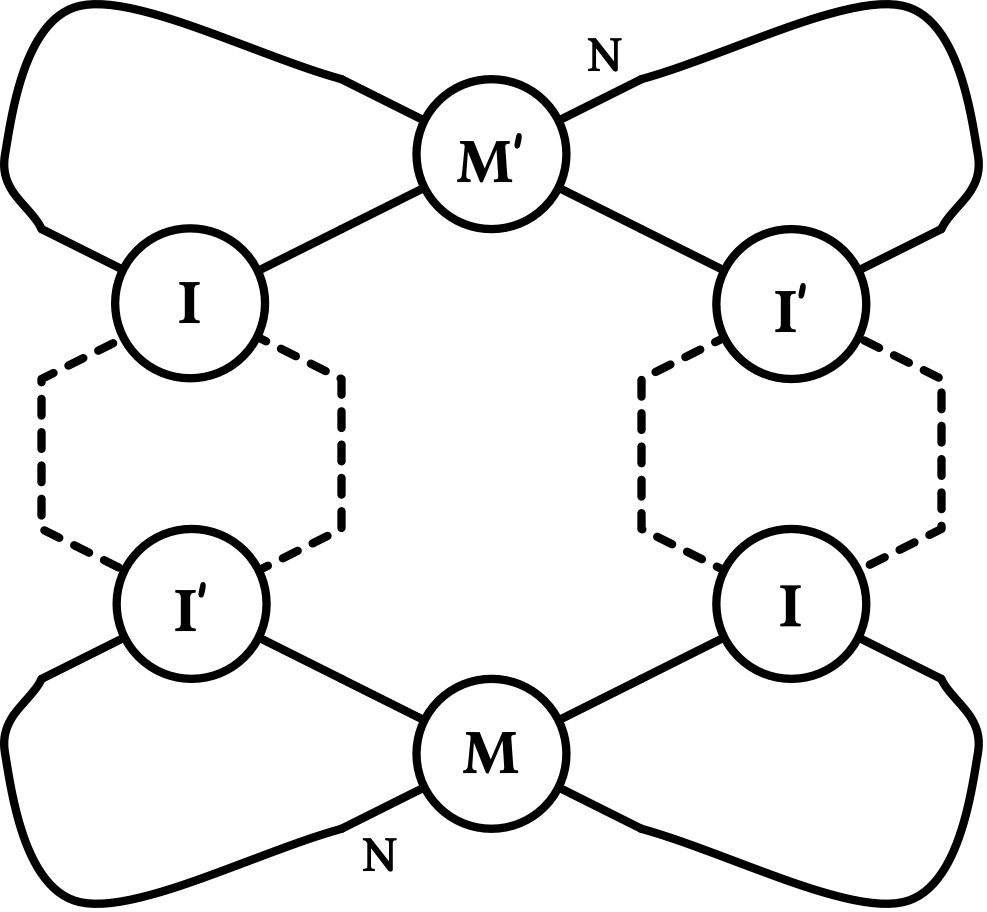
a

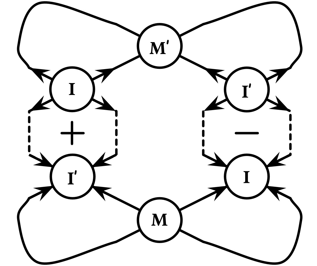
b

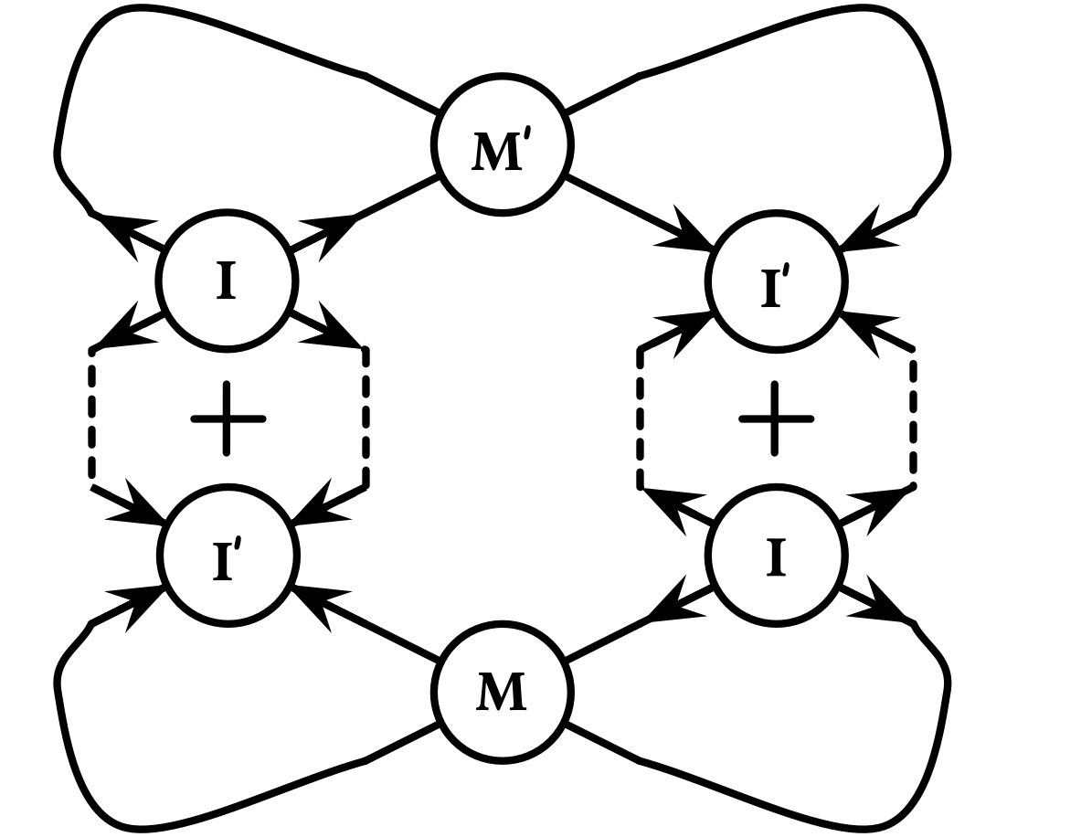
c

Figure 13: Modifying the four-way connection for the case when $d>a+b+c$.

Note that in the case when $a>b+c+d$ (or symmetrically $b>a+c+d$, $c>a+b+d$), the construction $G^{\prime}$ in the eight-vertex model is bipartite for any (not necessarily bipartite) 3-MAX CUT instance $G$. To see this, just check that (1) the amplifiers are bipartite and (2) the four way connections and the locking devices are bipartite by setting the nodes marked with $M,I,J,K$ on one side and the nodes marked with $M^{\prime},I^{\prime},J^{\prime},K^{\prime}$ on the other side. Therefore, approximately computing $Z(a,b,c,d)$ in these cases is NP-hard even on bipartite graphs. We remark this is no longer true for the construction of $G^{\prime}$ in the case when $d>a+b+c$. ∎

Lemma 5.2.

Let $(a_{k},b_{k},c_{k},d_{k})=\Lambda^{(k)}(a,b,c,d)$ given by (5.1). Assuming $a_{0}>b_{0}+c_{0}+d_{0}$, $a_{0},d_{0}>0$, and $b_{0},c_{0}\geq 0$, there exists some constants $\alpha>0,\beta>1$ depending only on $a_{0},b_{0},c_{0},d_{0}$ such that for all $k\geq 1$, $\frac{a_{k}}{b_{k}+c_{k}+d_{k}}\geq\alpha\beta^{2^{k}}$.

Proof.

Let $(a^{\prime},b^{\prime},c^{\prime},d^{\prime})=\Lambda(a,b,c,d)$ for any $a,b,c,d$ such that $a,d>0$ and $b,c\geq 0$. We have $a^{\prime}>0,b^{\prime},c^{\prime},d^{\prime}\geq 0$ and $b^{\prime}+c^{\prime}+d^{\prime}>0$. One can check that $\frac{a^{\prime}}{b^{\prime}+c^{\prime}+d^{\prime}}>\frac{a}{b+c+d}$ for any such $(a,b,c,d)$. One can check that

$$\frac{a^{\prime}}{b^{\prime}+c^{\prime}+d^{\prime}}-{\left(\frac{a}{b+c+d}\right)}^{2}=\frac{a(a-(b+c+d))F}{{(b+c+d)}^{2}(b^{\prime}+c^{\prime}+d^{\prime})},$$

where $F=(b^{2}+c^{2}+d^{2}+2bc+2bd+2cd)a^{5}+F_{4}a^{4}+F_{3}a^{3}+F_{2}a^{2}+F_{1}a+F_{0}$ and $F_{i}\ (0\leq i\leq 4)$ are polynomials only in $b,c,d$ (with not necessarily positive coefficients).

Therefore, when $\frac{a}{b+c+d}$ is sufficiently large, $\frac{a^{\prime}}{b^{\prime}+c^{\prime}+d^{\prime}}-{\left(\frac{a}{b+c+d}\right)}^{2}>0$. This indicates that the series $\left\{\frac{a_{k}}{b_{k}+c_{k}+d_{k}}\right\}_{k\geq 1}$ has a growth rate of $2^{k}$ after some finite $j$ such that $\frac{a_{j}}{b_{j}+c_{j}+d_{j}}$ is sufficiently large. If we normalize $a=1$, then $\Lambda$ takes a tuple $(\tilde{b},\tilde{c},\tilde{d})$ with $\tilde{b},\tilde{c},\tilde{d}\geq 0$ and $0<\tilde{b}+\tilde{c}+\tilde{d}\leq 1$ and maps it to another tuple $(\tilde{b^{\prime}},\tilde{c^{\prime}},\tilde{d^{\prime}})$ with $\tilde{b^{\prime}}+\tilde{c^{\prime}}+\tilde{d^{\prime}}<\tilde{b}+\tilde{c}+\tilde{d}$. The existence of such a point $j$ is proved in Lemma 5.3. This completes the proof by setting $\beta=\frac{a_{j}}{b_{j}+c_{j}+d_{j}}>1$. ∎

Lemma 5.3.

Let $\Delta=\{(b,c,d)\ |\ b,c,d\geq 0,b+c+d\leq 1\}$. Let $s:\Delta\rightarrow\mathbb{R}_{+}$ be the summation function $s((b,c,d))=b+c+d$. Suppose $g:\Delta\rightarrow\Delta$ is a continuous function such that for any $x\neq\mathbf{0}$, $s(g(x))<s(x)$. Then for any $\epsilon>0$, there exists $N\in\mathbb{Z}_{+}$ such that for any $x\in\Delta$, $s(g^{(N)}(x))<\epsilon$.

Proof.

For any $\epsilon>0$, let $\Delta_{\epsilon}=\{(b,c,d)\in\Delta\ |\ b+c+d\geq\epsilon\}$, and consider the continuous function $h(x)=s(x)-s(g(x))$ on $\Delta_{\epsilon}$. Since $\Delta_{\epsilon}$ is compact, $h$ reaches its minimum at some $x_{0}$ on $\Delta_{\epsilon}$. Since $h(x)>0$ for any $x\in\Delta_{\epsilon}$, we have $h(x_{0})>0$. Let $N=\lceil\frac{1}{h(x_{0})}\rceil$. Starting from any $x\in\Delta$, we claim that $s(g^{(N)}(x))<\epsilon$. If not, then $s(g^{(N)}(x))\geq\epsilon$, and by monotonicity, $g^{(n)}(x)\in\Delta_{\epsilon}$ for all $0\leq n\leq N$. But then $s(g^{(N)}(x))\leq s(x)-Nh(x_{0})\leq 0$, a contradiction. ∎

References

[Bax71]
R. J. Baxter.
Eight-vertex model in lattice statistics.
Phys. Rev. Lett., 26:832–833, Apr 1971.
[Bax72]
R. J. Baxter.
Partition function of the eight-vertex lattice model.
Annals of Physics, 70(1):193 – 228, 1972.
[Bax82]
R. J. Baxter.
Exactly Solved Models in Statistical Mechanics.
Academic Press Inc., San Diego, CA, USA, 1982.
[BN98]
G. T. Barkema and M. E. J. Newman.
Monte carlo simulation of ice models.
Phys. Rev. E, pages 1155–1166, 1998.
[CF17]
Jin-Yi Cai and Zhiguo Fu.
Complexity classification of the eight-vertex model.
CoRR, abs/1702.07938, 2017.
[CLL19]
Jin-Yi Cai, Tianyu Liu, and Pinyan Lu.