Equation of motion approach to black-box quantization: taming the multi-mode Jaynes-Cummings model

Abstract

An accurate modeling of a Josephson junction that is embedded in an arbitrary environment is of crucial importance for qubit design. We present a formalism to obtain a Lindblad master equation that describes the evolution of the system. As the qubit degrees of freedom oscillate with a well-defined frequency $\omega_{q}$, the environment only has to be modeled close to this frequency. Different from alternative approaches, we show that this goal can be achieved by modeling the environment with only few degrees of freedom. We treat the example of a transmon qubit coupled to a stripline resonator. We derive the parameters of a dissipative single-mode Jaynes-Cummings model starting from first principles. We show that the leading contribution of the off-resonant modes is a correlated decay process involving both the qubit and the resonator mode. In particular, our results show that the effect of the off-resonant modes in the multi-mode Jaynes-Cummings model is perturbative in $1/\omega_{q}$.

I Introduction

The theory of open quantum systems is needed to describe measurements or dissipation of a small quantum system such as a qubit. The most common approach is to use a Lindblad master equation.nielsen This equation is local in time due to the fact that the density of states of the environment is considered to be featureless and the coupling weak.breuer The main advantage of the Lindblad equation compared to more general approachesleggett:87 is that it directly describes the evolution of the reduced density matrix of the system without the need to solve for the environmental degrees of freedom. The study of systems that are coupled to more realistic (linear) environments is of immediate relevance for a better understanding of quantum systems. In this case, the dynamics of the environment is important and has to be treated appropriately.

For superconducting qubits, there has been recently a lot of interest in investigating and understanding quite general environments. If the environment is purely reactive, an equivalent circuit consists only of inductances and capacitances and can be quantized explicitly via one of the standard methods. devoret:96 ; burkard:04 ; ulrich:16 ; ansari:18 More importantly, a rather general approach called black-box quantization has been put forward recently for circuits with weak dissipation.nigg:12 A related method that works for arbitrary strong dissipation that relies on results in impedance synthesis has been proposed in Refs. solgun:14, ; solgun:15, . Based on this method it was also shown in Ref. solgun:17, that, considering the multi-port setting, the parameters in the Hamiltonian can be fundamentally related to the elements of the impedance matrix. All these methods have in common that a proper quantum description of the environment involves many degrees of freedom.

These results do not follow the physical expectation that for a good qubit at most a few degrees of freedom of the environment will be relevant. The physical intuition is even in contrast to recent findings that the multi-mode Jaynes-Cummings model differs considerably from its single-mode approximation.malekakhlagh:16 ; malekakhlagh:17 ; gely:17 ; parra:18 There is thus a clear need for a general formalism that allows to extract a few relevant degrees of freedom of the environment and treats the rest in an effective Lindbladian way.

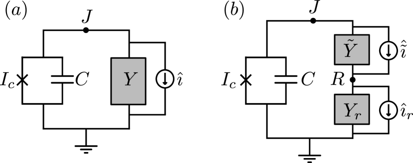
Figure 1: ($a$) Setup of a qubit (consisting of a capacitance $C$ and a Josephson junction with critical current $I_{c}$) coupled to an arbitrary environment described by the admittance $Y_{\omega}$. In particular, we are interested in cases where the admittance is small and is almost constant close to the frequency $\omega_{q}$ of the qubit. ($b$) If the latter condition is not fulfilled, we go over to an equivalent description of the system where the single admittance is replaced by two admittances $\tilde{Y}_{\omega}$ and $Y_{r,\omega}$ in series, such that $Y^{-1}=\tilde{Y}^{-1}+Y_{r}^{-1}$. The idea is that $Y_{r}$ is the admittance of a single bosonic mode and captures the frequency dependence whereas the (remaining) admittance $\tilde{Y}$ has a weaker frequency dependence.

Here, we address this question: we present results for a superconducting qubit that is embedded in a low admittance environment. We describe a self-consistent procedure that decides if and how many modes have to be extracted from the environment in order to obtain a good approximation of the dynamics of the system. We show that due to the fact that in a qubit both the voltage and the current fluctuate with the qubit frequency, the dynamics of the environment only has to be accurately modeled close to this frequency. In particular, we discuss the case of a featureless environment and the case where there is a single relevant degree of freedom. We obtain explicit expressions of the resulting Lindblad equation as a function of the admittance of the environment. As an example, we treat a transmon qubit that is capacitively coupled to a stripline resonator. We derive the effective parameters of a dissipative Jaynes-Cummings model involving the qubit and a single resonant mode of the cavity. We show that all the off-resonant modes can be treated perturbatively. In particular, we find that the main effect of the off-resonant modes is a correlated noise involving both the resonator and the cavity. Moreover, we show that our formalism is capable of analytically describing the asymmetric line-shape of the qubit decay rate that has been found in Ref. houck:08, .

The paper is organized as follows. In Sec. II we introduce the setup of a Josephson junction in parallel with an arbitrary admittance. Considering the problem in the Heisenberg picture, we obtain the equation of motion for the system operators. After projecting the equation of motion onto the relevant qubit subspace and within the assumption that the environment only weakly perturbs the qubit, we derive our central result, the approximate equation of motion, Eq. (8), satisfied by the qubit. In Sec. III, we introduce the admittance of a lossy stripline resonator that serves as a concrete application for our general formalism throughout the paper. The case in which the qubit is off-resonant with all the modes of the environment (dispersive regime) is treated in Sec. IV. In this case, the effect of the modes is just to cause a shift of the qubit frequency as well as a decay which are connected to the imaginary and real part of the admittance, respectively. In Sec. V, we consider the case in which the qubit is close to a resonance of one of the environmental modes. We explicitly show how the resonant mode can be split off from the environment while still taking the effect of the off-resonant modes into account. In particular, we obtain an effective Jaynes-Cummings model where all the parameters are expressed in terms of the admittance of the general environment. We confirm our results providing a comparison with numerical calculations in Sec. VI. The conclusions are finally drawn in Sec. VII.

II System

We are interested in modeling a Josephson junction coupled to an arbitrary environment. We denote the phase difference across the junction by $\varphi(t)$ which is related to the voltage by the Josephson relation $V(t)=(\hbar/2e)\dot{\varphi}(t)$ with $\hbar$ the reduced Planck’s constant and $e>0$ the elementary charge. We describe the influence of the linear environment by an admittance $Y(t)$ that relates the voltage $V(t)$ to the current $I_{e}(t)$ through the environment via

$$I_{e}(t)=\int_{-\infty}^{\infty}Y(t-t^{\prime})V(t^{\prime})\,dt^{\prime}=(Y\star V)(t).$$ (1)

Due to causality, its Fourier transform, given by $Y_{\omega}=\int e^{i\omega t}Y(t)dt$, is analytic with no poles or zeros in the upper half plane.triverio:07 The real (imaginary) part of $Y_{\omega}$ describes the dissipation (reactance). As the environment is assumed to be linear the equation (1) is also the correct relation between the current operator $\hat{I}_{e}$ and the voltage operator $\hat{V}$ in the Heisenberg picture.

Kirchhoff’s current law at the node $J$ in Fig. 1 demands that

$$\frac{\hbar C}{2e}\ddot{\hat{\varphi}}(t)+I_{c}\sin\hat{\varphi}(t)+\frac{\hbar}{2e}(Y\star\dot{\hat{\varphi}})(t)=\hat{\imath}(t)$$ (2)

with $C$ ($I_{c}$) the capacitance (critical current) of the Josephson junction and $\hat{\imath}$ the noise due to the dissipative part of $Y$. Equation (2) is Heisenberg’s equation of motion for the phase variable $\hat{\varphi}(t)$. The noise is characterized by the commutation relationzoller

$$[\hat{\imath}(t),\hat{\imath}(t^{\prime})]=i\hbar\frac{d}{dt}[Y(t-t^{\prime})+Y(t^{\prime}-t)].$$ (3)

Assuming that the dissipative elements of the environment (E) are well-thermalized at a temperature $T$, the fluctuations are Gaussian random variables with zero mean and a variance

$$\tfrac{1}{2}\langle\{\hat{\imath}^{\dagger}_{\omega},\hat{\imath}_{\omega^{\prime}}\}\rangle_{\text{E}}=2\pi\hbar\omega\operatorname{Re}(Y_{\omega})(2\bar{n}_{\omega}+1)\delta(\omega-\omega^{\prime}),$$ (4)

where $\{\hat{A},\hat{B}\}=\hat{A}\hat{B}+\hat{B}\hat{A}$ denotes the anticommutator and $\bar{n}_{\omega}=(e^{\hbar\omega/k_{B}T}-1)^{-1}$ is the mean photon number.

Equation (2) is valid for a Josephson junction coupled to an arbitrary linear environment. It is a true black-box equation, as the environment only enters via its admittance and the associated noise term. However, the equation is a non-linear stochastic operator equation for which there are no clear solution strategies. In the following, we will make a set of controlled assumptions in which we extract a few relevant degrees of freedom that evolve according to a Lindblad master equation. In particular, we are interested in the situation where Eq. (2) describes the dynamics of a qubit that is weakly perturbed by the environment which is achieved in the small admittance setting. The specific requirements is given in Eq. (18) and will be discussed below.

We first treat the environment as an open circuit ($Y=0$) and solve the equation

$$\frac{\hbar C}{2e}\ddot{\hat{\varphi}}(t)+I_{c}\sin\hat{\varphi}(t)=0;$$ (5)

note that this is the Heisenberg equation associated with the Hamiltonian

$$\hat{H}_{q}=-\frac{2e^{2}}{C}\frac{\partial^{2}}{\partial\varphi^{2}}-\frac{\hbar I_{c}}{2e}\cos(\varphi).$$ (6)

We assume that the dynamics only involves the two lowest eigenstates $|g,e\rangle$ at frequencies $\omega_{g,e}$. For the Hamiltonian $\hat{H}_{q}$ the two lowest eigenstates have opposite parity with respect to $\hat{\varphi}\mapsto-\hat{\varphi}$ such that the phase operator is off-diagonal in the eigenbasis. As a result, at $Y=0$, Eq. (5) is solved by

$$\hat{\varphi}(t)=\varphi_{0}\Bigl{[}e^{-i\omega_{q}t}\hat{\sigma}^{-}(t)+e^{i\omega_{q}t}\hat{\sigma}^{+}(t)\Bigr{]}.$$ (7)

for constant $\hat{\sigma}^{\pm}(t)\equiv\hat{\sigma}^{\pm}$ with $\varphi_{0}=\langle e|\hat{\varphi}|g\rangle$ and $\omega_{q}=\omega_{e}-\omega_{g}$; here and below, it will be convenient to parameterize the amplitude $\varphi_{0}$ of the phase fluctuation defining the characteristic impedance of the qubit $Z_{q}=\hbar\varphi_{0}^{2}/2e^{2}$ and introduce the effective qubit capacitance $C_{q}=(\omega_{q}Z_{q})^{-1}$.

At weak dissipation, we can thus employ a variant of the rotating wave approximation (RWA) in which we assume that $\hat{\sigma}^{\pm}_{\eta}$ contains only frequency components with $|\eta|\ll\omega_{q}$. For concreteness, we denote with $\bar{\eta}$ the typical frequency above which $\hat{\sigma}^{\pm}_{\eta}$ vanishes. In Appendix A, we show that with the ansatz (7) the projection of (2) onto the relevant qubit degrees of freedom leads to the equation of motion (valid for $\bar{\eta}\ll\omega_{q}$)

$$-2(\hat{\sigma}^{z}\partial_{t}\hat{\sigma}^{-})_{\eta}+\omega Z_{q}Y_{\omega}\hat{\sigma}^{-}_{\eta} =i\sqrt{\frac{2Z_{q}}{\hbar}}\hat{\imath}_{\omega}$$ (8)

in frequency space; here, $\eta=\omega-\omega_{q}$ is the frequency measured with respect to the qubit frequency. In the following, we will show how Eq. (8) can be used to analyze the influence of the environment on the qubit in a few cases. In particular, the goal is to render Eq. (8) into an equation that is local in time and thus can be related to a Lindblad master equation.

In order that the approach taken above is valid, a few assumptions have to be made about the environment. At first, we need that $\mathop{\rm Im}Y_{\omega}\to 0$ for $\omega\to 0$. This excludes the case of a shunting inductance (as in the fluxonium qubit) investigated in Ref. koch:09, ; smith:16, . Moreover, as we will see below, we need that $|Y_{\omega_{q}}|Z_{q}\ll 1$. In particular, this can be violated if there is an additional capacitance in the environment. In fact if $Z_{q}\mathop{\rm Im}Y_{\omega_{q}}\simeq 1$, we should extract a capacitance from the environment and add it to $C$ before continuing with the approach, see also below.

III Single- and multi-mode approximation of a stripline resonator

In the previous section, we have obtained our central result Eq. (8), which, under RWA, is valid for a general admittance. In order to fix ideas, we connect our general formalism to a concrete physical setup of a transmon qubit that is capacitively coupled to a stripline resonator whose admittance is introduced in this section. We will find a more and more refined effective Liouvillian description in the reminder of the paper. In particular, we want to show how all the modes of the stripline resonator (forming the environment) can be naturally incorporated and that there is a perturbative procedure to go beyond the single-mode approximation. For low dissipation, the admittance of the resonator is approximately given by

$$Y_{\text{mm}}=-\frac{2iC_{r}\omega_{0}}{\pi}\tan\left[\frac{\pi(\omega+\tfrac{i}{2}\kappa)}{\omega_{0}}\right]$$ (9)

with $\omega_{0}$ the fundamental frequency of the resonator, $\kappa$ the damping rate, and $C_{r}$ the characteristic capacitance of the resonator; see App. B. The modes of the resonator are at $\omega_{n}=n\omega_{0}$ with $n\in\mathbb{N}$. Including the coupling capacitance, the total impedance of the environment is given by $Y^{-1}=Y^{-1}_{c}+Y^{-1}_{\text{mm}}$ with $Y_{c}=-i\omega C_{c}$. As we will see in the following, the coupling capacitance $C_{c}$ (assumed to be small) is proportional to the coupling rate $g$ of the Jaynes-Cummings Hamiltonian.

If we assume that the qubit frequency is close to the frequency of mode $n_{0}$, i.e., $|\Delta|<\omega_{0}$ with the detuning $\Delta=\omega_{q}-\omega_{n_{0}}$, we can approximate the admittance by a single mode ($\omega>0$)

$$Y_{r} =-2iC_{r}(\omega-\omega_{r}+\tfrac{1}{2}i\kappa)$$ (10)

with $\omega_{r}=\omega_{n_{0}}$. This corresponds to the positive frequency response of an RLC circuit with a capacitance $C_{r}$, a resistance $R_{r}=(C_{r}\kappa)^{-1}$, and an inductance $L_{r}=(C_{r}\omega_{r}^{2})^{-1}$ in parallel. Note that close to the resonance with $\kappa,|\omega-\omega_{r}|\ll\omega_{0}$, the single-mode approximation is a very good approximation to the total admittance. In particular, one can model the stripline as the single mode $Y_{r}$ in series with another admittance of value $\tilde{Y}=(Y^{-1}-Y^{-1}_{r})^{-1}$. For small coupling ($C_{c}\ll C_{r}$), we find the expansion

$$\tilde{Y}=(Y^{-1}-Y^{-1}_{r})^{-1} \approx Y_{c}+Y_{c}^{2}(Y_{r}^{-1}-Y_{\text{mm}}^{-1})$$

$$\approx-i\omega C_{c}+\frac{\pi^{2}\omega^{2}C_{c}^{2}\kappa}{12\omega_{0}^{2}C_{r}}$$ (11)

valid close to the resonance frequency; the first term describes the influence of the coupling capacitance whereas the second term captures the leading contribution of the influence of all the modes that are off-resonant. Its effect is dissipative and will lead to the decay constant $\gamma$ in the Jaynes-Cummings model.

IV Dispersive regime

Having set the stage by presenting the central result as well as our concrete physical application, we will show how to derive a Lindblad master equation for the case when the qubit is detuned from all the resonances of the environment, i.e., we treat the case of a general though off-resonant environment. In this case, we can assume that the admittance is constant over the relevant frequency range $[\omega_{q}-\bar{\eta},\omega_{q}+\bar{\eta}]$. As a result (provided that $\bar{\eta}\ll\omega_{q}$), Eq. (8) becomes local in time and assumes the simple form

$$\partial_{t}\hat{\sigma}^{-}(t)+\tfrac{1}{2}\omega_{q}Z_{q}Y_{\omega_{q}}\hat{\sigma}^{-}(t)=\sqrt{\omega_{q}Z_{q}\operatorname{Re}(Y_{\omega_{q}})}\,\hat{\sigma}^{z}(t)\hat{b}(t)$$ (12)

of a quantum Stratonovich stochastic differential equation; here, we have introduced a new operator $\hat{b}(t)$ via

$$\hat{\imath}(t)=i\sqrt{2\hbar\omega_{q}\operatorname{Re}(Y_{\omega_{q}})}e^{-i\omega_{q}t}\hat{b}(t)$$ (13)

The operator $\hat{b}(t)$ is a quantum white noise with $[\hat{b}(t),\hat{b}^{\dagger}(t^{\prime})]=\delta(t-t^{\prime})$, $[\hat{b}(t),\hat{b}(t^{\prime})]=0$,

$$\langle\{\hat{b}(t),\hat{b}^{\dagger}(t^{\prime})\}\rangle_{\text{E}}=(2\bar{n}+1)\delta(t-t^{\prime}),$$ (14)

and $\langle\{\hat{b}(t),\hat{b}(t^{\prime})\}\rangle_{\text{E}}=0$ with $\bar{n}=\bar{n}_{\omega_{q}}$.

By inspecting the left hand side of Eq. (12), we immediately observe that the environment leads to a frequency shift (also called Lamb-shift)

$$\delta\omega_{q}=\tfrac{1}{2}\omega_{q}Z_{q}\operatorname{Im}(Y_{\omega_{q}})$$ (15)

and a decay rate (also called Purcell rate)

$$\gamma=\omega_{q}Z_{q}\operatorname{Re}(Y_{\omega_{q}});$$ (16)

see also Ref. esteve:86, ; houck:08, ; bronn:15, ; scheer:18, . As the equation of motion (including the noise) is local in time, it is equivalent to the Lindblad equation

$$\dot{\rho}=-\frac{i}{2}\delta\omega_{q}[\hat{\sigma}_{z},\rho]+\gamma(\bar{n}+1)\mathcal{D}[\hat{\sigma}^{-}](\rho)\\ +\gamma\bar{n}\mathcal{D}[\hat{\sigma}^{+}](\rho)$$ (17)

for the density matrix of the qubit; here, we have introduced the superoperator $\mathcal{D}[\hat{J}](\rho)=\hat{J}\rho\hat{J}^{\dagger}-\tfrac{1}{2}\{\hat{J}^{\dagger}\hat{J},\rho\}$ corresponding to the jump operator $\hat{J}$. Now, we can formulate (self-consistently) when the dispersive approximation is applicable. Indeed, we have that $\bar{\eta}\approx\max\{|\delta\omega_{q}|,\gamma\}$. As a result, the approach is valid as long as the admittance does not change appreciably on the scale $\bar{\eta}$; i.e., Eq. (17) is valid as long as the self-consistency equation

$$\frac{dY_{\omega_{q}}}{d\omega}\,\max\{|\delta\omega_{q}|,\gamma\}\ll Y_{\omega_{q}}$$ (18)

is fulfilled.

For the concrete example of stripline resonator, introduced in Sec. III, we can use the expansion

$$Y=Y_{c}-\frac{Y_{c}^{2}}{Y_{\text{mm}}}$$ (19)

valid for weak coupling with $|Y_{c}/Y_{\text{mm}}|\approx C_{c}/C_{r}\ll 1$. The first term in (19) corresponds to a capacitance in parallel to the junction capacitance. Its effect can be taken (exactly) into account by replacing $C_{q}\mapsto C_{q}+C_{c}$. The nontrivial effects of the environment solely arise from the second term. The admittance changes on the scale $\Delta$ such that for self-consistency, we have to require that $|\delta\omega_{q}|,\gamma\ll|\Delta|$. For the stripline resonator, we obtain the expressions

$$\delta\omega_{q}=\frac{\pi g^{2}\sin(2\pi\Delta/\omega_{0})}{\omega_{0}[\cosh(\pi\kappa/\omega_{0})-\cos(2\pi\Delta/\omega_{0})]},$$ (20)

$$\gamma=\frac{2\pi g^{2}\sinh(\pi\kappa/\omega_{0})}{\omega_{0}[\cosh(\pi\kappa/\omega_{0})-\cos(2\pi\Delta/\omega_{0})]};$$ (21)

here, we have introduced the coupling rate

$$g=\frac{C_{c}}{2\sqrt{C_{q}C_{r}}}\omega_{q}$$ (22)

which will later be shown to be the coupling constant of the Jaynes-Cummings model. Note that we have consciously defined the coupling rate different from the more common choice, with $\omega_{q}$ replaced by the symmetric expression $\sqrt{\omega_{r}\omega_{q}}$. The reason is twofold. First, we consider an initial situation where the qubit is excited while the resonator is still in its equilibrium state. Due to this, it is more natural to evaluate the environment at the qubit frequency. Second, due to this definition, the simple expressions in (23) and (24) are valid all the way up to order $(\Delta,\kappa)^{4}/\omega_{0}^{4}$ which is not true for the alternative definition.

In the expressions (20) and (21) still all the modes of the stripline resonator have been included. The only assumptions so far are weak coupling ($C_{c}\ll C_{r}$), small shifts ($|\delta\omega_{q}|,\gamma\ll|\Delta|$), and weak damping ($\kappa\ll\omega_{0}$). For the case of small detuning ($\Delta\ll\omega_{0}$), the expressions (20) and (21) can be further simplified to

$$\delta\omega_{q} =\frac{g^{2}\Delta}{\Delta^{2}+(\kappa/2)^{2}}-\frac{\pi^{2}g^{2}\Delta}{3\omega_{0}^{2}},$$ (23)

$$\gamma =\frac{g^{2}\kappa}{\Delta^{2}+(\kappa/2)^{2}}+\frac{\pi^{2}g^{2}\kappa}{3\omega_{0}^{2}}$$ (24)

with a correction term only appearing in order $1/\omega_{0}^{4}$. Note that the single-mode approximation corresponds to the first terms and the effect of all the other modes is captured perturbatively by the second term. The present approach gives a perturbative expansion in the small parameters and avoids the rediagonalization of the complete system as in Ref. gely:17, . In this expansion, the conventional single-mode approximation corresponds to the first term,blais:04 with all the remaining modes contributing to a small correction of order $\omega_{0}^{-2}$.

V Resonant regime

In the previous section, we have treated the simplest case of a dispersive qubit-environment coupling. In this case, the admittance does not vary too much close to the qubit frequency and we can simply replace it by a constant. A more elaborate analysis is necessary in the case where the shift is so large that the admittance cannot be assumed to be constant and Eq. (18) is violated. In particular, in the case of a small admittance, this can only happen when there is a root of the admittance (in the complex plane at $\omega_{*}$) close to the frequency of the qubit. Let us parameterize the root in question by $\omega_{*}=\omega_{r}-i\kappa/2$ and introduce the characteristic capacitance $C_{r}=\frac{i}{2}(dY/d\omega)_{\omega=\omega_{*}}$. The admittance close to the qubit frequency is then well approximated by a single mode $Y_{r}$. We assume that the remaining admittance $\tilde{Y}=(Y^{-1}-Y^{-1}_{r})^{-1}$ does not change appreciably over the range $\bar{\eta}$, i.e., that (18) is satisfied for $\tilde{Y}$ (even though it does not hold for $Y$ itself). Otherwise, the process of extracting a mode can be repeated until this assumption is fulfilled.

The resonant mode corresponds to an RLC circuit. We associate with this circuit a bosonic mode $\hat{a}$. Moreover, we extend the equation of motion to incorporate this mode. In particular, we have the equations of motion (for the nodes $J$ and $R$ in Fig. 1)

$$-2(\hat{\sigma}^{z}\partial_{t}\hat{\sigma}^{-})_{\eta}+\omega Z_{q}\tilde{Y}_{\omega}\biggl{(}\hat{\sigma}^{-}_{\eta}-\sqrt{\frac{C_{q}}{C_{r}}}\,\hat{a}_{\eta}\biggr{)}=i\sqrt{\frac{2Z_{q}}{\hbar}}\,\hat{\tilde{\imath}}_{\omega}\;,$$ (25)

$$-2iC_{r}(\eta+\Delta+\tfrac{i}{2}\kappa)\hat{a}_{\eta}+\tilde{Y}_{\omega}\biggl{(}\hat{a}_{\eta}-\sqrt{\frac{C_{r}}{C_{q}}}\,\hat{\sigma}^{-}_{\eta}\biggr{)}$$

$$\qquad\qquad\qquad\qquad\qquad\qquad=i\sqrt{\frac{2C_{r}}{\hbar\omega_{q}}}(\hat{\imath}_{r,\omega}-\hat{\tilde{\imath}}_{\omega})$$ (26)

where $\hat{\tilde{\imath}}$ ($\hat{\imath}_{r}$) corresponds to the noise due to $\operatorname{Re}\tilde{Y}$ ($\operatorname{Re}Y_{r}$). It can be checked by a straightforward calculation that solving (26) for $\hat{a}_{\eta}$ and inserting the resulting expression into (25) that (8) is recovered, see App. C. The advantage of the new representation is that the frequency dependence of $\tilde{Y}$ around the qubit frequency is milder than the one of $Y$. In particular, provided that $\tilde{Y}$ does not change appreciably on the scale $\bar{\eta}$, we can replace $\omega$ by $\omega_{q}$ and arrive at the system of equations

$$\partial_{t}\hat{\sigma}^{-}(t)+\frac{\tilde{Y}_{\omega_{q}}}{2C_{q}} \biggl{[}\hat{\sigma}^{-}(t)+\sqrt{\frac{C_{q}}{C_{r}}}\hat{\sigma}^{z}(t)\hat{a}(t)\biggl{]}$$

$$=\sqrt{C_{q}^{-1}\operatorname{Re}\tilde{Y}_{\omega_{q}}}\,\hat{\sigma}^{z}(t)\hat{\tilde{b}}(t),$$ (27)

$$(\partial_{t}-i\Delta+\tfrac{1}{2}\kappa)\hat{a}(t) +\frac{\tilde{Y}_{\omega_{q}}}{2C_{r}}\biggl{[}\hat{a}(t)-\sqrt{\frac{C_{r}}{C}}\hat{\sigma}^{-}(t)\biggr{]}$$

$$=\sqrt{C_{r}^{-1}\operatorname{Re}\tilde{Y}_{\omega_{q}}}\,\hat{\tilde{b}}(t)-\sqrt{\kappa}\,\hat{b}_{r}(t)$$ (28)

that are local in time.

The coherent evolution is generated by the Jaynes-Cummings Hamiltonian

$$\hat{H}_{\text{JC}}=\tfrac{1}{2}\delta\omega_{q}\hat{\sigma}_{z}+(\delta\omega_{r}-\Delta)\hat{a}^{\dagger}\hat{a}+g(\hat{\sigma}^{+}\hat{a}+\hat{a}^{\dagger}\hat{\sigma}^{-}),$$ (29)

with the parameters

$$\delta\omega_{q}=\frac{\operatorname{Im}(\tilde{Y}_{\omega_{q}})}{2C_{q}},\;\delta\omega_{r}=\frac{\operatorname{Im}(\tilde{Y}_{\omega_{q}})}{2C_{r}},\;g=-\frac{\operatorname{Im}(\tilde{Y}_{\omega_{q}})}{2\sqrt{C_{q}C_{r}}},$$ (30)

corresponding to the frequency shift of the qubit, the frequency shift of the resonator, and the coherent coupling rate. Transforming the quantum Stratonovich stochastic differential equations (V) and (V) to an equivalent Lindblad equation yields

$$\dot{\rho}=-i[\hat{H}_{\text{JC}},\rho] +\kappa(\bar{n}+1)\mathcal{D}[\hat{a}](\rho)+\kappa\bar{n}\mathcal{D}[\hat{a}^{\dagger}](\rho)$$

$$+\gamma(\bar{n}+1)\mathcal{D}\Bigl{[}\hat{\sigma}^{-}-\sqrt{\frac{C_{q}}{C_{r}}}\hat{a}\Bigr{]}(\rho)$$

$$+\gamma\bar{n}\mathcal{D}\Bigl{[}\hat{\sigma}^{+}-\sqrt{\frac{C_{q}}{C_{r}}}\hat{a}^{\dagger}\Bigr{]}(\rho)$$ (31)

with the decay rate

$$\gamma =\frac{\operatorname{Re}(\tilde{Y}_{\omega_{q}})}{C_{q}}.$$ (32)

This rate corresponds to a correlated decay process involving both the qubit as well as the oscillator. The master equation is valid as long as the self-consistency equation (18) is fulfilled where $Y$ is replaced by $\tilde{Y}$.

The Eq. (V) is the master equation of a Josephson junction coupled to a general environment. For the concrete example of a stripline resonator, we can use the expression (III) when the qubit is brought close to the $n_{0}$-th resonance of the resonator at the frequency $\omega_{r}$. In this case, the parameters of the Jaynes-Cummings model assume the form

$$\delta\omega_{q} =-\frac{C_{c}\omega_{q}}{2C_{q}}, \delta\omega_{r} =-\frac{C_{c}\omega_{q}}{2C_{r}}, g =\frac{C_{c}\omega_{q}}{2\sqrt{C_{q}C_{r}}}.$$ (33)

The qubit frequency shift and the coherent coupling corresponds to the first term expansion in $C_{c}$ of the results presented in Sec. IV. The leading contribution of the off-resonant modes is given by the correlated decay with a rate

$$\gamma=\frac{\pi^{2}g^{2}\kappa}{3\omega_{0}^{2}};$$ (34)

this is the leading effect of the off-resonant modes in the multi-mode resonator cf. Eq. (24); to the best of our knowledge, the correlated decay has never been discussed before in the literature.

VI Comparison to numerics

In this section, we would like to compare the results of Sec. IV to the numerical approaches of Refs. houck:08, ; gely:17, . The numerical approaches are designed to work in the transmon regime with $I_{c}\gg e^{3}/\hbar C$. In this regime, the Josephson junction acts as an inductance $L_{J}=2e/\hbar I_{c}$ as we can use the approximate equality $I_{c}\sin\phi\approx I_{c}\phi$ in Eq. (2). With this, the total system becomes linear and thus several solution strategies are available.

The admittance approach of Ref. houck:08, , directly solves for the eigenmodes of the complete system by seeking the roots of the total admittance

$$Y_{C}+Y_{J}+Y=0$$ (35)

as a function of $\omega$; here, $Y_{C}=-i\omega C$ and $Y_{L}=(-i\omega L_{J})^{-1}$ are the admittances of the capacitance and the linearized Josephson junction respectively. The approach works for reactive as well as for dissipative environments. For each solution $\omega_{*}$, the real part denotes the frequency and the imaginary part the decay rate. As long as the admittance of the environment is small, there is a solution close to the bare qubit frequency which is plotted in Fig. 2. This approach is in principle very close to our presentation in Sec. IV. However, crucially our approach works also outside the transmon regime where the total system is not approximately harmonic. In Fig. 2, it can be seen that the analytical results Eqs. (20) and (23) describe the behavior rather well. In particular, the simple expression (23) captures the asymmetry of the decay rate due to the higher modes that has been observed in Ref. houck:08, .

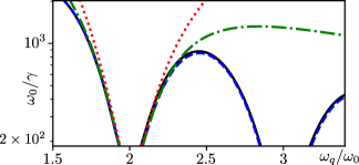
Figure 2: Dimensionless relaxation time $\omega_{0}/\gamma^{-1}$ of a qubit due to the multi-mode environment with $C_{c}/C_{r}=0.02$, $C_{c}/C=0.02$, and $\kappa/\omega_{0}=0.2$ as a function of the qubit frequency $\omega_{q}$. The solid line is the numerics given by the admittance approach of Ref. houck:08, . The plot shows $\gamma=-2\operatorname{Im}(\omega_{*})$. The dashed line is the result of Eq. (21). The dash-dotted line is the approximate expression (24) with $\omega_{r}=2\omega_{0}$. The dotted line is the single-mode approximation (first term of (24)). It can be seen that the analytical formulas describe the decay rate rather well. In particular (24) reproduces the asymmetry in the decay rate that has been observed in Ref. houck:08, .

The rediagonalization approach of Ref. gely:17, on the other hand, concentrates on reactive environments. It proceeds by finding new eigenmodes of the stripline resonator (=environment) once they are coupled to the qubit. For completeness, we show the procedure in App. D. The result are a set of frequencies $\nu_{n}$ and coupling constants $g_{n}$ which allow for treating the system as a multi-mode Jaynes-Cummings model. Note that we do not have $\nu_{n}=n\omega_{0}$ anymore. The Lamb shift then gets a contribution of all the eigenmodes which act independently. In particular, we find

$$\delta\omega_{q}=\sum_{n=0}^{\infty}\frac{g_{n}^{2}}{\Delta_{n}(1-\Delta_{n}/2\omega_{q})}$$ (36)

with $\Delta_{n}=\omega_{q}-\nu_{n}$. In Fig. 3, we show that there is an (approximate) sum rule associated with the new eigenmodes. In particular, the contribution of all the modes (Eq. (36)) approximately gives the result $g^{2}/\Delta$ of the bare single mode Jaynes-Cummings model. Moreover, we find that the contribution of the remaining modes is well captured by the second term in Eq. (23).

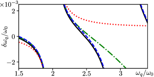
Figure 3: Lamb shift: The parameters are chosen as in Fig. 2 with $\kappa=0$. The solid line shows the numerical result of the rediagonlization approach of Ref. gely:17, , i.e., Eq. (36). Note that our analytical results, Eq. (20) (dashed line) and Eq. (23) (dash-dotted line), reproduce the numerical results rather well. Even the single-mode approximation, first term (23) (dotted line), is valid close to the resonance which indicates that Eq. (36) is approximately given by the naïve result $g^{2}/\Delta$.

VII Conclusion

In conclusion, we have presented a general approach to derive an effective Lindblad equation for a superconducting qubit embedded in an arbitrary linear environment with a small admittance. The approach yields an effective model where the qubit is coupled to a few harmonic degrees of freedom of the environment. For the case of a single relevant environmental mode, we have given explicit expressions of the model parameters (coupling constant, decay rates, jump operators) as a function of the admittance. In particular, we have found that the single-mode Jaynes-Cummings model is the leading term in the description of a superconducting qubit that is coupled to a multi-mode resonator. The main effect of the off-resonant modes is a novel, correlated decay that involves both the resonator and the qubit degrees of freedom. In particular, our results show that the multi-mode Jaynes-Cummings model does not only have a cutoff free description but that the correction of the off-resonant modes can be obtained analytically in a perturbative expansion in $1/\omega_{0}\simeq 1/\omega_{q}$. It is an interesting idea for further studies to extend our results to the case of a fluxonium qubit. In this case, the environment has a large admittance with $Z_{q}|Y_{\omega}|\gg 1$ such that an perturbative approach using the impedance $Z_{\omega}=1/Y_{\omega}$ instead of the admittance seems to be the appropriate as a starting point.

Appendix A Derivation of Eq. (8)

In this Appendix, we give a more rigorous derivation of Eq. (8) using the formalism developed in Chap. 3 of Ref. zoller, . We start by considering the Hamiltonian of a transmon coupled linearly to a linear environment that without loss of generality can be assumed to be a collection of harmonic oscillators. The Hamiltonian of the total system can be taken as

$$\hat{H}=\hat{H}_{q}(\hat{Q},\hat{\Phi})+\tfrac{1}{2}\sum_{n}\Bigl{[}(\hat{p}_{n}-\kappa_{n}\hat{\Phi})^{2}+\omega_{n}^{2}\hat{q}_{n}^{2}\Bigr{]},$$ (37)

with the system (qubit) Hamiltonian

$$\hat{H}_{q}=\frac{\hat{Q}^{2}}{2C}-E_{J}\cos\biggl{(}\frac{2\pi}{\Phi_{0}}\hat{\Phi}\biggr{)};$$ (38)

note that this definition is equivalent to Eq. (6) with $\hat{\varphi}=2\pi\hat{\Phi}/\Phi_{0}$, $\Phi_{0}=h/2e$, and $I_{c}=2\pi E_{J}/\Phi_{0}$. We further impose the following commutation relations for the bath

$$[\hat{p}_{n},\hat{p}_{m}]=[\hat{q}_{n},\hat{q}_{m}]=0,$$ (39a)

$$[\hat{q}_{n},\hat{p}_{m}]=i\hbar\delta_{nm},$$ (39b)

and for the system

$$[\hat{\Phi},\hat{Q}]=i\hbar,$$ (40)

while any system operators commutes with any bath operator. These commutation relations will hold true between operators in the Heisenberg picture at the same time. Following Ref. zoller, , we can show that from the Hamiltonian Eq. (37), our Eq. (2) follows, with the admittance in the time domain identified as

$$Y(t)=\begin{cases}0,\quad t<0,\\ \sum_{n}\kappa_{n}^{2}\cos(\omega_{n}t),\quad t\geq 0,\end{cases}$$ (41)

which is manifestly causal, and the noise current term

$$\hat{\imath}(t)=i\sum_{n}\kappa_{n}\sqrt{\frac{\hbar\omega_{n}}{2}}\hat{a}_{n}^{\dagger}(t_{0})+\text{H.c.}$$ (42)

with the annihilation operator of the $n$-th harmonic oscillator $\hat{a}_{n}=(\omega_{n}\hat{q}_{n}+i\hat{p}_{n})/\sqrt{2\hbar\omega_{n}}$ and $\hat{a}_{n}^{\dagger}$ its Hermitian conjugate.

After these identifications we perform the two level approximation by projecting the system Hamiltonian and the operator $\Phi$ onto the first two levels. This leads to the following substitutions

$$\hat{H}_{q}(\hat{\Phi},\hat{Q}) \mapsto\tfrac{1}{2}\hbar\omega_{q}\hat{\sigma}^{z}, \hat{\Phi} \mapsto\sqrt{\tfrac{1}{2}\hbar Z_{q}}\;\hat{\sigma}^{x}.$$ (43)

in the Hamiltonian Eq. (37). We then obtain the spin-boson Hamiltonianleppakangas:18

$$\hat{H}=\tfrac{1}{2}\hbar\omega_{q}\hat{\sigma}^{z}+\tfrac{1}{2}\sum_{n}(\hat{p}_{n}^{2}+\omega_{n}^{2}\hat{q}_{n}^{2})-\sqrt{\frac{\hbar Z_{q}}{2}}\hat{\sigma}^{x}\sum_{n}\kappa_{n}\hat{p}_{n},$$ (44)

where we have neglected constant terms. The Heisenberg equation of motion for a generic qubit operator $\hat{A}_{q}$ under the Hamiltonian Eq. (44) reads

$$\frac{d\hat{A}_{q}(t)}{dt}=\tfrac{i}{2}\omega_{q}[\hat{\sigma}^{z}(t),\hat{A}_{q}(t)]\\ -i\sqrt{\frac{Z_{q}}{2\hbar}}[\hat{\sigma}^{x}(t),\hat{A}_{q}(t)]\sum_{n}\kappa_{n}\hat{p}_{n}(t),$$ (45)

where we have used the fact that the operator $\sum_{n}\kappa_{n}\hat{p}_{n}(t)$ commutes with any system operator at the same time. Following Ref. zoller, , we also obtain

$$\sum_{n}\kappa_{n}\hat{p}_{n}(t)=\hat{\imath}(t)-\sqrt{\frac{\hbar Z_{q}}{2}}\int_{t_{0}}^{t}\!\!dt^{\prime}\frac{dY(t-t^{\prime})}{dt^{\prime}}\hat{\sigma}^{x}(t^{\prime});$$ (46)

in what follows, we will neglect the transient behavior and let $t_{0}\to-\infty$. We want to obtain the Heisenberg equation of motion for the operator $\hat{\sigma}^{-}(t)$. From Eq. (45), we readily obtain

$$\partial_{t}\hat{\sigma}^{-}(t)+i\omega_{q}\hat{\sigma}^{-}(t)-\tfrac{i}{2}Z_{q}\sigma^{z}(t)\int\!dt^{\prime}\frac{dY(t-t^{\prime})}{dt^{\prime}}\hat{\sigma}^{x}(t^{\prime})\\ =-i\sqrt{\frac{Z_{q}}{2\hbar}}\hat{\sigma}^{z}(t)\hat{\imath}(t).$$ (47)

Going over to a rotating frame with $\hat{\sigma}^{-}\mapsto\hat{\sigma}^{-}e^{-i\omega_{q}t}$, like in Eq. (7), yields

$$e^{-i\omega_{q}t}\hat{\sigma}^{z}(t)\partial_{t}\hat{\sigma}^{-}(t)-\tfrac{i}{2}Z_{q}\int\!dt^{\prime}\frac{dY(t-t^{\prime})}{dt^{\prime}}\\ \times[e^{-i\omega_{q}t^{\prime}}\hat{\sigma}^{-}(t^{\prime})+\text{H.c.}]=-i\sqrt{\frac{Z_{q}}{2\hbar}}\hat{\imath}(t).$$ (48)

Taking the Fourier transform, we obtain

$$-(\hat{\sigma}^{z}\partial_{t}\hat{\sigma}^{-})_{\eta}\!+\!\tfrac{1}{2}\omega Z_{q}Y_{\omega}\bigl{(}\hat{\sigma}_{\eta}^{-}+\hat{\sigma}_{\omega+\omega_{q}}^{+}\bigr{)}\!=\!i\sqrt{\frac{Z_{q}}{2\hbar}}\hat{\imath}_{\omega},$$ (49)

Now neglecting the term proportional to $\hat{\sigma}_{\omega+\omega_{q}}^{+}$ consistently with the approximation described in the text we finally obtain Eq. (8).

The result of the Appendix can be summarized as follows: in the two-level approximation, the current $\hat{I}_{q}=\hbar C\ddot{\hat{\varphi}}/2e+I_{c}\sin\hat{\varphi}$ that is flowing through the qubit assumes the form

$$\hat{I}_{q}(t)=i\sqrt{\frac{2\hbar}{Z_{q}}}\;\hat{\sigma}^{z}(t)\partial_{t}\hat{\sigma}^{-}(t)+\text{H.c.}$$ (50)

with $\sigma^{-}$ in the rotating frame. This result can be used in the equation of motion (2) to project it onto the qubit subspace.

Appendix B Admittance of a multi-mode stripline resonator

The admittance of a transmission line or stripline which is shunted by a load with admittance $Y_{L}$ is given bypozar

$$Y_{\text{tl}}=Z_{0}^{-1}\frac{Z_{0}Y_{L}-i\tan(\pi\omega/\omega_{0})}{1-iZ_{0}Y_{L}\tan(\pi\omega/\omega_{0})}$$ (51)

with $Z_{0}$ the characteristic impedance of the transmission line and $\omega_{0}$ the fundamental frequency. We are interested in the situation where the transmission line forms a good (multi-mode) resonator. In this case, we have that $|Y_{L}|Z_{0}\ll 1$ and we can use the expansion

$$Y_{\text{tl}}=-iZ_{0}^{-1}\tan(\pi\omega/\omega_{0})+Y_{L}$$ (52)

where we have made use of the fact that the second term is only relevant when $\tan(\pi\omega/\omega_{0})\ll 1$. We also can use the alternative expression $Y_{\text{tl}}=-iZ_{0}^{-1}\tan[\pi(\omega+i\kappa_{\omega}/2)/\omega_{0}]$ with

$$\kappa_{\omega}=\frac{2\omega_{0}Z_{0}Y_{L}}{\pi}$$ (53)

valid to the same order. Here, we have made explicit that in principle $\kappa_{\omega}$ depends on frequency via $Y_{L}$. However, as it is only important to accurately describe the admittance close to qubit frequency, we can approximately set $\omega=\omega_{q}$ in Eq. (53). For concreteness, we require $C_{L}\omega_{q}R\gg 1$ in order to obtain Eq. (9) with

$$\kappa=\frac{2\omega_{0}Z_{0}}{\pi R}\qquad\text{and}\qquad C_{r}=\frac{\pi}{2\omega_{0}Z_{0}}.$$ (54)

For typical experiments, this regime is not obtained. As a result the decay rate of the modes depends on the modenumber houck:08 . Our approach also works in this regime, however the results are not so nice as the admittance is not given by (1) but rather $\kappa$ becomes frequency dependent.

Appendix C Integrating out the resonator

In this appendix, we would like to show that the equations (25) and (26) are equivalent to (8) after the resonator mode $\hat{a}_{\eta}$ has been integrated out and thus the node $R$ eliminated. Solving (26) for $\hat{a}_{\eta}$ yields

$$\hat{a}_{\eta}=\frac{\tilde{Y}_{\omega}\sqrt{\frac{C_{r}}{C}}\,\hat{\sigma}^{-}_{\eta}+i\sqrt{\frac{2C_{r}}{\hbar\omega_{q}}}(\hat{\imath}_{r,\omega}-\hat{\tilde{\imath}}_{\omega})}{Y_{r,\omega}+\tilde{Y}_{\omega}}.$$ (55)

Plugging this expression into (25), we obtain (8) with $Y^{-1}=Y_{r}^{-1}+\tilde{Y}^{-1}$ and

$$\hat{\imath}_{\omega}=\frac{\tilde{Y}_{\omega}\hat{\imath}_{r,\omega}+Y_{r,\omega}\hat{\tilde{\imath}}}{Y_{r,\omega}+\tilde{Y}_{\omega}}.$$ (56)

Due to the relation

$$\operatorname{Re}(Y_{\omega})=\frac{|\tilde{Y}_{\omega}|^{2}\operatorname{Re}(Y_{r,\omega})+|\tilde{Y}_{r,\omega}|^{2}\operatorname{Re}(\tilde{Y}_{\omega})}{|Y_{r,\omega}+\tilde{Y}_{\omega}|^{2}}.$$ (57)

and the fact that $\hat{\imath}_{r,\omega}$ and $\hat{\tilde{\imath}}$ are distributed according to Eqs. (3) and (4) with $Y$ replaced by $Y_{r}$ and $\tilde{Y}_{\omega}$, it can be shown that $\hat{\imath}$ has the correct commutation relation and expectation value.

Appendix D Rediagonalization approach

In this section, we present the rediagonalization approach of Ref. gely:17, for the stripline resonator. However, for convenience, we diagonalize the system already on the Lagrangian level and not on the Hamiltonian as in Ref. gely:17, .

The Lagrangian of the qubit coupled to a stripline resonator (with $\kappa=0$) is given by

$$\mathcal{L} =\frac{C+C_{c}}{2}\dot{\varphi}^{2}+\frac{\hbar I_{c}}{2e}\cos(\varphi)-C_{c}\dot{\varphi}\sum_{\mu=0}^{\infty}\dot{\phi}_{\mu}+\mathcal{L}_{r},$$ (58)

$$\mathcal{L}_{r} =C_{r}\dot{\phi}_{0}^{2}+\sum_{\mu=1}^{\infty}\left(\frac{C_{r}\dot{\phi}_{\mu}^{2}}{2}-\frac{\phi_{\mu}^{2}}{2L_{\mu}}\right)+\frac{C_{c}}{2}\left(\sum_{\mu=0}^{\infty}\dot{\phi}_{\mu}\right)^{2}\,,$$

where $L_{\mu}=(\mu^{2}C_{r}\omega_{0}^{2})^{-1}$ for $\mu\in\mathbb{N}$. That this is the correct description of the environment, can be seen by the expansion

$$Y^{-1}_{\text{mm}} =\frac{\pi i}{2C_{r}\omega_{0}}\cot(\pi\omega/\omega_{0})$$

$$=(-iC_{r}\omega)^{-1}\left[\frac{1}{2}+\sum_{\mu=1}^{\infty}\left(1-\frac{\mu^{2}\omega_{0}^{2}}{\omega^{2}}\right)^{-1}\right]$$ (59)

which in circuit terms corresponds to a capacitance in series with an infinite ladder of LC-resonators.

The method proceeds by finding the eigenmodes of the resonator Lagrangian $\mathcal{L}_{r}$ including the coupling capacitance $C_{c}$. In particular, we would like to find eigensolutions to the Euler-Langrange equations

$$(C_{r}+C_{c})\ddot{\phi}_{\mu}+L_{\mu}^{-1}\phi_{\mu}+C_{c}\sum_{\lambda\neq\mu}\ddot{\phi}_{\lambda}=0$$ (60)

with $\phi_{\mu}(t)=e^{-i\nu t}v_{\mu}$. This corresponds to the generalized eigenvalues problem $A\bm{v}=\nu^{2}B\bm{v}$ where $A$ is diagonal with $A_{\mu\lambda}=L_{\mu}^{-1}\delta_{\mu\lambda}$ and $B_{\mu\lambda}=C_{r}\delta_{\mu\lambda}+C_{c}+C_{r}\delta_{\mu 0}\delta_{\lambda 0}$.

From the general theory of symmetric generalized eigenvalue problems with positive definite matrices, it is known that the eigenvalues $\nu_{n}^{2}$ are positive (thus we can choose $\nu_{n}\geq 0$) and that the eigenvectors can be normalized such that

$${\bm{v}}_{n}\cdot B{\bm{v}}_{m}=C_{r}\delta_{nm}$$ (61)

Thus, introducing the new modes $\psi_{n}(t)$ with

$$\bm{\phi}(t)=\sum_{n=0}^{\infty}\psi_{n}(t)\bm{v}_{n}$$ (62)

the Lagrangian assumes the diagonal form

$$\mathcal{L}=\frac{C+C_{c}}{2}\dot{\varphi}^{2}+\frac{\hbar I_{c}}{2e}\cos(\varphi)-\dot{\varphi}\sum_{n=0}^{\infty}C_{n}\dot{\psi}_{n}\\ +\frac{C_{r}}{2}\sum_{n=0}^{\infty}(\dot{\psi}_{n}^{2}-\nu_{n}^{2}\psi_{n}^{2})$$ (63)

with the coupling capacitance

$$C_{n}=C_{c}\sum_{\mu=0}^{\infty}(\bm{v}_{n})_{\mu}$$ (64)

to the $n$-eigenmode.

In order to define coupling strength $g_{n}$, the authors of Ref. gely:17, propose to treat the case of a qubit in the transmon regime. In this case, the Josephson junction effectively acts as an inductance. The coupling strength to the $n$-th mode can be identified with

$$g_{n}=\frac{C_{n}\omega_{q}}{2\sqrt{(C+C_{c})C_{r}}},$$ (65)

see Eq. (22). Note that crucially, the strength now depends on $n$ as $C_{n}$ is not simply $C_{c}$. The equations of motion are given by

$$(C+C_{c})(\ddot{\varphi}+\omega_{q}^{2}\varphi) =\sum_{n=0}^{\infty}C_{n}\ddot{\psi}_{n},$$ (66)

$$C_{r}(\ddot{\psi}_{n}+\nu_{n}^{2}\psi_{n}) =C_{n}\ddot{\varphi}.$$ (67)

Going over to frequency space and solving for the mode $\psi_{n}$, we obtain

$$\psi_{n,\omega}=\frac{C_{n}\omega^{2}\varphi_{\omega}}{C_{r}(\omega^{2}-\nu_{n}^{2})}\,.$$ (68)

The qubit equation Eq. (66) involves only frequencies close to the qubit frequency. Assuming that all the frequencies $\nu_{n}$ are sufficiently detuned from the qubit frequency $\omega_{q}$, we can replace $\omega\mapsto\omega_{q}$ in Eq. (68). Plugging this into the Eq. (66), we obtain

$$0 =\ddot{\varphi}+\omega_{q}^{2}\left(1+\sum_{n=0}^{\infty}\frac{4g^{2}_{n}}{\omega_{q}^{2}-\nu_{n}^{2}}\right)\varphi$$

$$\approx\ddot{\varphi}+\left(\omega_{q}+\sum_{n=0}^{\infty}\frac{2\omega_{q}g^{2}_{n}}{\omega_{q}^{2}-\nu_{n}^{2}}\right)^{2}\varphi,$$ (69)

i.e, the shift due to the different modes is independent as announced by Ref. gely:17, .

Numerically, the procedure is as follows. The number of modes in Eq. (58) is made finite with $\mu\leq N$. Then the generalized eigenvalue problem is solved on a computer. The eigenenergies $\nu_{n}$ as well as the coupling constants $g_{n}$ are calculated. As the different eigenmodes act independently, the Lamb shift is approximately given by the sum of the Lamb shifts of the individual modes, i.e.,

$$\delta\omega_{q}=\sum_{n=0}^{\infty}\frac{2\omega_{q}g_{n}^{2}}{\omega_{q}^{2}-\nu_{n}^{2}}=\sum_{n=0}^{\infty}\frac{g_{n}^{2}}{\Delta_{n}(1-\Delta_{n}/2\omega_{q})}$$ (70)

with $\Delta_{n}=\omega_{q}-\nu_{n}$. Note that due to the fact that some of the modes are highly detuned, we could not use the approximation

$$\frac{2\omega_{q}}{\omega_{q}^{2}-\nu_{n}^{2}}=\frac{1}{\Delta_{n}}$$ (71)

that is commonly used in the dispersive regime with $\Delta_{n}\ll\omega_{q}$.

References

- (1) M. A. Nielsen and I. L. Chuang, Quantum Computation and Quantum Information (Cambridge University Press, Cambridge, 2000).
- (2) H.-P. Breuer and F. Petruccione, The Theory of Open Quantum Systems (Oxford University Press, New York, 2007).
- (3) A. J. Leggett, S. Chakravarty, A. T. Dorsey, M. P. A. Fisher, A. Garg, and W. Zwerger, Dynamics of the dissipative two-states system, Rev. Mod. Phys. 59, 1 (1987).
- (4) M. H. Devoret, Quantum fluctuations in electrical circuits, in Les Houches Session LXIII, edited by S. Reynaud, E. Giacobino, and J. Zinn-Justin (Elsevier, Amsterdam, 1996).
- (5) G. Burkard, R. H. Koch, and D. P. DiVincenzo, Multi-level quantum description of decoherence in superconducting qubits, Phys. Rev. B 69, 064503 (2004).
- (6) J. Ulrich and F. Hassler, Dual approach to circuit quantization using loop charges, Phys. Rev. B 94, 094505 (2016).
- (7) M. H. Ansari, Exact quantization of superconducting circuits, arxiv:1807.00792 (2018).
- (8) S. E. Nigg, H. Paik, B. Vlastakis, G. Kirchmair, S. Shankar, L. Frunzio, M. Devoret, R. Schoelkopf, and S. Girvin, Black-box superconducting circuit quantization, Phys. Rev. Lett. 108, 240502 (2012).
- (9) F. Solgun, D. W. Abraham, and D. P. DiVincenzo, Blackbox quantization of superconducting circuits using exact impedance synthesis, Phys. Rev. B 90, 134504 (2014).
- (10) F. Solgun and D. P. DiVincenzo, Multiport impedance quantization, Ann. Phys. (NY) 361, 605 (2015).
- (11) F. Solgun, D. P. DiVincenzo, and J. M. Gambetta, Simple impedance response formulas for the dispersive interaction rates in the effective hamiltonians of low anharmonicity superconducting qubits, arXiv:1712.08154 (2017).
- (12) M. Malekakhlagh and H. E. Türeci, Origin and implications of an -like contribution in the quantization of circuit-QED systems, Phys. Rev. A 93, 012120 (2016).
- (13) M. Malekakhlagh, A. Petrescu, and H. E. Türeci, Cutoff-free circuit quantum electrodynamics, Phys. Rev. Lett. 119, 073601 (2017).
- (14) M. F. Gely, A. Parra-Rodriguez, D. Bothner, Y. M. Blanter, S. J. Bosman, E. Solano, and G. A. Steele, Convergence of the multimode quantum Rabi model of circuit quantum electrodynamics, Phys. Rev. B 95, 245115 (2017).
- (15) A. Parra-Rodriguez, E. Rico, E. Solano, and I. Egusquiza, Quantum networks in divergence-free circuit QED, Quantum Sci. Technol. 3, 024012 (2018).
- (16) We refer to the term proportional to in Eq. (V). It is interesting that the leading effect of the off-resonant modes is dissipative, see Eq. (III).
- (17) A. A. Houck, J. A. Schreier, B. R. Johnson, J. M. Chow, J. Koch, J. M. Gambetta, D. I. Schuster, L. Frunzio, M. H. Devoret, S. M. Girvin, and R. J. Schoelkopf, Controlling the spontaneous emission of a superconducting transmon qubit, Phys. Rev. Lett. 101, 080502 (2008).
- (18) P. Triverio, S. Grivet-Talocia, M. S. Nakhla, F. G. Canavero, and R. Achar, Stability, causality, and passivity in electrical interconnect models, IEEE Trans. Adv. Packag. 30, 795 (2007).
- (19) Note the different convention with respect to the electrical engineering literature. In particular, the admittance of a capacitance is given by .
- (20) C. W. Gardiner and P. Zoller, Quantum Noise (Springer-Verlag, Berlin, 2000).
- (21) Of course, we have that .
- (22) Note that in the transmon limit the qubit capacitance coincides with the geometric capacitance .
- (23) J. Koch, V. Manucharyan, M. H. Devoret, and L. I. Glazman, Charging effects in the inductively shunted josephson junction, Phys. Rev. Lett. 103, 217004 (2009).
- (24) W. C. Smith, A. Kou, U. Vool, I. M. Pop, L. Frunzio, R. J. Schoelkopf, and M. H. Devoret, Quantization of inductively shunted superconducting circuits, Phys. Rev. B 94, 144507 (2016).
- (25) See Sec. 3.4.5 of Ref. zoller, .
- (26) D. Esteve, M. H. Devoret, and J. M. Martinis, Effect of an arbitrary dissipative circuit on the quantum energy levels and tunneling of a Josephson junction, Phys. Rev. B 34, 158 (1986).
- (27) N. T. Bronn, E. Magesan, N. A. Masluk, J. M. Chow, J. M. Gambetta, and M. Steffen, Reducing spontaneous emission in circuit quantum electrodynamics by a combined read- out/filter technique, IEEE Trans. Appl. Supercond. 25, 1700410 (2015).
- (28) M. G. Scheer and M. B. Block, Computational modeling of decay and hybridization in superconducting circuits, arXiv:1810.11510 (2018).
- (29) Our derivation of the Lindblad equation does not include the ac-Stark shift which is typically unimportant. A more refined calculation leads to (17) with as the prefactor of the first term proportional to .carmichael1
- (30) In general, one can always include the effect of a capacitance of value exactly and only treat the remaining admittance as the environment.
- (31) A. Blais, R.-S. Huang, A. Wallraff, S. M. Girvin, and R. J. Schoelkopf, Cavity quantum electrodynamics for superconducting electrical circuits: an architecture for quantum computation, Phys. Rev. A 69, 062320 (2004).
- (32) Note that for weak dissipation the capacitance is always real.
- (33) J. Leppäkangas, J. Braumüller, M. Hauck, J.-M. Reiner, I. Schwenk, S. Zanker, L. Fritz, A. V. Ustinov, M. Weides, and M. Marthaler, Quantum simulation of the spin-boson model with a microwave circuit, Phys. Rev. A 97, 052321 (2018).
- (34) D. M. Pozar, Microwave Engineering (Wiley, New York, 2011).
- (35) H. Carmichael, Statistical Methods in Quantum Optics 1: Master Equations and Fokker-Planck Equations (Springer, Berlin, 1999).