Fundamental parameter accuracy of DA and DB white dwarfs in Gaia Data Release 2

Abstract

We report on a comparison of spectroscopic analyses for hydrogen (DA) and helium atmosphere (DB) white dwarfs with Gaia Data Release 2 (DR2) parallaxes and photometry. We assume a reddening law and a mass-radius relation to connect the effective temperatures ($T_{\rm eff}$) and surface gravities ($\log g$) to masses and radii. This allows the comparison of two largely independent sets of fundamental parameters for 7039 DA and 521 DB stars with high-quality observations. This subset of the Gaia white dwarf sample is large enough to detect systematic trends in the derived parameters. We find that spectroscopic and photometric parameters generally agree within uncertainties when the expectation of a single star is verified. Gaia allows the identification of a small systematic offset in the temperature scale between the two techniques, as well as confirming a small residual high-mass bump in the DA mass distribution around 11 000-13 000 K. This assessment of the accuracy of white dwarf fundamental parameters derived from Gaia is a first step in understanding systematic effects in related astrophysical applications such as the derivation of the local stellar formation history, initial-to-final mass relation, and statistics of evolved planetary systems.

1 Introduction

The atmospheric parameters of white dwarfs, the effective temperature ($T_{\rm eff}$) and surface gravity ($\log g$), play a fundamental role in the study of post-main-sequence stellar evolution (see, e.g., Kalirai et al., 2014; Rolland et al., 2018), evolved planetary systems (Koester et al., 2014), Galactic formation history (Tremblay et al., 2014), and the calibration of instruments (Bohlin et al., 2014). For decades, the most precise method to determine $T_{\rm eff}$ and $\log g$ has been the spectroscopic fitting of the Balmer lines in hydrogen-atmosphere DA white dwarfs (Bergeron et al., 1992; Finley et al., 1997), and the He I lines in helium-dominated DB stars (Beauchamp et al., 1999; Voss et al., 2007; Bergeron et al., 2011). In contrast, trigonometric parallax measurements of stellar remnants or their companions can also be used to characterise $T_{\rm eff}$ and stellar radii from photometric analyses (Koester et al., 1979; Bergeron et al., 2001). The surface gravity can then be inferred by using the white dwarf mass-radius relation (see, e.g., Fontaine et al., 2001), with a small dependence on the assumed internal stratification (Romero et al., 2012). The main advantage of the photometric technique is that it can be used to fit cool DC white dwarfs with no optical transitions as well as metal- or carbon-rich remnants where spectroscopic $\log g$ determinations are difficult (Dufour et al., 2005, 2007b). One shortcoming is that for $T_{\rm eff}\gtrapprox 12\,000$ K, optical colours of all stellar remnants get rather insensitive to the temperature, requiring very precise photometry for that determination (Carrasco et al., 2014). Until now, the main limitation of the photometric analyses has been that precise parallax measurements were available for only hundreds of white dwarfs (Bédard et al., 2017), compared to the $\approx$ 30 000 objects (Kleinman et al., 2013; Kepler et al., 2015, 2016; Gentile Fusillo et al., 2018) with spectroscopy from the Sloan Digital Sky Survey (SDSS; Abazajian et al., 2009).

The spectroscopic and photometric techniques have been combined to derive masses and radii independent of a theoretical mass-radius relation (Vauclair et al., 1997; Provencal et al., 1998; Holberg et al., 2012; Tremblay et al., 2017; Bédard et al., 2017). This method aims at understanding the internal stratification of white dwarfs, where additional constraints from asteroseismology (Romero et al., 2012) and statistical analyses (Tremblay & Bergeron, 2008) can also be considered. The cornerstone European Space Agency Gaia space mission is now challenging our knowledge of white dwarfs by providing a homogeneous and extremely precise sample of photometry and parallaxes. Tremblay et al. (2017) used 52 directly or indirectly (wide companions) observed white dwarfs in Gaia Data Release 1 and found that uncertainties on the spectroscopic parameters are now the dominant uncertainties on individual mass and radius determinations for bright and close white dwarfs. The authors conclude that the comparison of the photometric and spectroscopic techniques is equally a verification of the mass-radius relation and the model atmospheres (see also Genest-Beaulieu & Bergeron 2014). In the latter case, a number of improvements have been made in recent years for the bulk of the white dwarfs that have H- or He-dominated atmospheres, such as Stark broadening for hydrogen lines including non-ideal gas effects (Tremblay & Bergeron, 2009), neutral broadening for Lyman $\alpha$ (Kowalski & Saumon, 2006), improved opacities from collision-induced-absorption (CIA; Blouin et al., 2017), and the account of 3D convective effects for both DA and DB stars (Tremblay et al., 2013; Cukanovaite et al., 2018). It is highly desirable to compare these theoretical developments with Gaia.

There are approximately 250 000 white dwarfs (Gentile Fusillo et al., 2018) in the second Gaia Data Release (DR2; Gaia Collaboration et al., 2018). The sample is estimated to be $95.8{+1.3\atop-1.7}$ percent volume-complete within 20 pc (Hollands et al., 2018), and this is likely to hold up to a distance of $\approx$ 60 pc, where the coolest disk white dwarfs become too faint to be observed (Gentile Fusillo et al., 2018). In addition to parallaxes that have a median precision of 1.5% within 100 pc, Gaia DR2 provides colours in the broad $G$, $G_{\rm BP}$, and $G_{\rm RP}$ pass bands, which can be used to constrain white dwarf parameters using the photometric technique (El-Badry et al., 2018; Jiménez-Esteban et al., 2018; Gentile Fusillo et al., 2018; Kilic et al., 2018). For the 20 pc sample, Hollands et al. (2018) have demonstrated that the atmospheric parameters derived from Gaia are in very good agreement with earlier photometric analyses. Furthermore, Gentile Fusillo et al. (2018) have shown that for known single DA white dwarfs for which the monochromatic spectral energy distribution is well modeled (Bohlin et al., 2014), Gaia-derived $T_{\rm eff}$ values are in very good agreement with independent photometric temperatures obtained using instead the Pan-STARRS (Chambers et al., 2016) or SDSS data sets. This suggests that Gaia photometry is well calibrated at the precision level of other existing photometric surveys.

In this work, we present an overview of how Gaia DR2 compares with published or existing spectroscopic parameters for single, non-magnetic DA and DB/DBA white dwarfs (Gianninas et al., 2011; Koester & Kepler, 2015; Tremblay et al., 2016; Rolland et al., 2018). These correspond to the spectral types where both the photometric and spectroscopic techniques are deemed reliable and independent. Gaia provides such a dramatic update in sample size compared to existing parallax samples that we can now hope to identify trends as a function of $T_{\rm eff}$, $\log g$ or spectral subtypes. Our initial approach is to combine the spectroscopic atmospheric parameters, a theoretical mass-radius relation, and the Gaia $G$ apparent magnitude to predict a parallax that can be compared with the observed value. In a further step, we also derive independent $T_{\rm eff}$ and $\log g$ values from the photometric technique using the full Gaia data set. In all cases we present the current picture and make no attempt to improve any of the existing models, data calibration, or fitting techniques.

In Section 2 we present our selected spectroscopic samples and in Section 3 we compare existing spectroscopic distances for DA and DB/DBA stars with Gaia parallaxes. In Section 4 we compare Gaia DR2 photometric atmospheric parameters to spectroscopic analyses, followed by a discussion in Section 5 and a summary in Section 6.

2 White Dwarf Samples

The all-sky and bright sample of DA white dwarfs from Gianninas et al. (2011) drawn from the White Dwarf Catalog of McCook & Sion (1999) is a benchmark to study their fundamental parameters because of the high signal-to-noise ratio (S/N) of the spectroscopic observations. The relative proximity of the objects also allows for the most precise Gaia data set that we employ in this study. We rely on the 1D atmospheric parameters as published by the authors. We also use a sample of DA white dwarfs drawn from the Gaia-SDSS catalogue of Gentile Fusillo et al. (2018). We have secured all spectra from the SDSS SkyServer with the new data reduction from DR14 (Abolfathi et al., 2018), and fitted the observations using the same technique and 1D model atmospheres as those employed for our analyses of earlier data releases (Tremblay et al., 2011; Tremblay et al., 2016) as well as Gianninas et al. (2011). In brief, the model atmospheres rely on the Stark broadening profiles of Tremblay & Bergeron (2009), the Hummer & Mihalas (1988) equation-of-state, and fully account for NLTE effects (Tremblay et al., 2011). For all objects where we observed the so-called Balmer-line problem (Werner, 1996; Gianninas et al., 2010) with deeper than predicted cores at H$\alpha$ and H$\beta$, we employed the NLTE models with carbon, nitrogen, and oxygen computed by Gianninas et al. (2010) to provide a better fit to the Balmer lines and improved atmospheric parameters (see Section 4.3 of Tremblay et al., 2011).

Table 1: White dwarf samples

Sample	Initial	Clean (non-magnetic,	Gaia DR2 (with
		single WDs, S/N $>$ 20)	quality cuts, Eqs. 1-3)
DA: Gianninas et al. (2011)	1265	1201	1145
DA: SDSS DR1-DR7	12491	2941	2726a
DA: SDSS BOSS DR9-DR14	8650	3584	3168b
DB: Rolland et al. (2018)	119	119	116
DB: Koester & Kepler (2015)	1107	439	405
a Spectroscopic parameters available in Table LABEL:A1.
b Spectroscopic parameters available in Table LABEL:A2.
Notes: Spectroscopic parameters are otherwise taken from the sample papers and Gaia data
from Gentile Fusillo et al. (2018).

From a visual inspection of the SDSS spectra and fits to the $ugriz$ photometry, we have cleaned the sample of magnetic white dwarfs, DAO stars, cool He-rich atmospheres with weak hydrogen lines, and identifiable binaries of the types DA+DC, DA+DB and DA+dM. For the Gianninas et al. (2011) sample, we have used the existing flags in their catalogue to filter these subtypes. We note that double DA white dwarfs can not be identified from the spectrum and photometry alone except for rare double-lined binaries (Tremblay et al., 2011). We kept all DAZ white dwarfs as the presence of metals does not significantly influence the atmospheric parameters. For SDSS spectra, we restrict our analysis to objects with S/N $>$ 20 since this high-quality subsample is cleaner and already large enough to provide a robust comparison with Gaia.

In the following, we split the SDSS spectra in two subsamples, first based on observations made with the original SDSS spectrograph (Abazajian et al., 2009) up to DR7. This subsample largely overlaps with the catalogue of Kleinman et al. (2013) apart from a small fraction of cool DA white dwarfs not covered by their colour cuts (Gentile Fusillo et al., 2018). The second sample, overlapping with Kepler et al. (2015, 2016), is for white dwarfs observed within the newer SDSS-III Baryon Oscillation Spectroscopic Survey (BOSS; Ahn et al., 2012), corresponding to the SDSS Data Releases 9 to 14. The adopted spectroscopic samples of DA white dwarfs are summarised in Table 1. We emphasise that by using the same models and fitting technique for all three data sets, we can more easily study the effects from the different instruments and data reduction.

We also perform a comparison of the spectroscopic parameters of DB and DBA white dwarfs with Gaia. We rely on the all-sky sample of bright objects from Rolland et al. (2018) and the SDSS DR12 analysis of Koester & Kepler (2015). In both cases we employ the published atmospheric parameters. As for the DA white dwarfs in the SDSS, we restrict the comparison to S/N $>$ 20 to provide a comparison with Gaia on the same scale as the other samples. Both DB samples already exclude magnetic white dwarfs, and therefore we make no additional modifications. We also make no distinction between the SDSS spectrographs in this case because the number of objects is much smaller (see Table 1) and the two adopted samples use different models and fitting techniques, meaning that isolating data reduction issues is much more difficult.

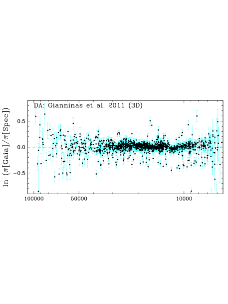
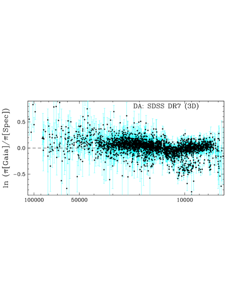
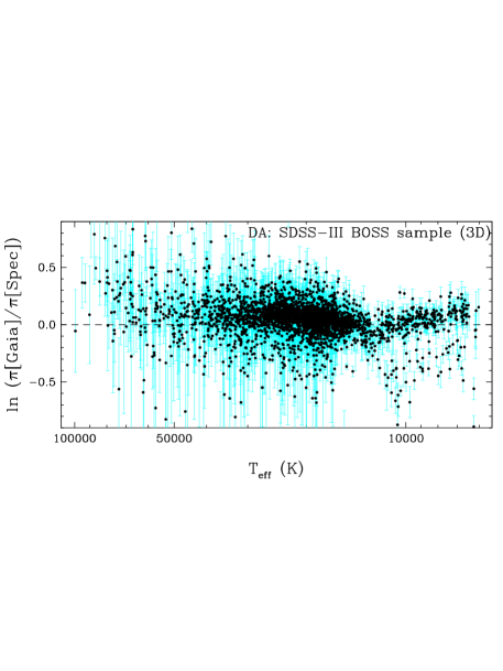
Figure 1: Natural logarithm of the ratio between observed Gaia DR2 and predicted spectroscopic parallaxes using 3D corrections for the samples of Gianninas et al. (2011) (top panel), SDSS DR7 (middle panel), and SDSS-III BOSS (bottom panel). We note that the natural logarithm of the ratio is close to the difference in percentage.

We have cross-matched our initial samples with the Gaia DR2 white dwarf catalogue of Gentile Fusillo et al. (2018). A number of Gaia sources have poor quality flags, and we made the following additional cuts

$$\textsc{astrometric\_excess\_noise}<0.75~{},$$ (1)

$$\textsc{phot\_bp\_rp\_excess\_factor}/$$

$$(1.3+0.06(G_{\rm BP}-G_{\rm RP})^{2})<1.0~{},$$ (2)

$$\textsc{astrometric\_sigma5d\_max}<1.0~{}.$$ (3)

The removal of a small fraction of lower quality data with likely underestimated Gaia errors does not significantly impact our analysis. We note that these cuts, coupled with the removal of DA+DC and DA+DB candidates based on a spectral visual inspection, implies that we have biases against detecting double degenerates in our adopted samples. Therefore, we make no attempt to derive the double degenerate fraction. The different samples are nevertheless a reasonable representation of the magnitude-limited local population of non-magnetic and apparently single white dwarfs, and completeness is not required to compare their fundamental parameters using different methods. The final number of white dwarfs with precise spectroscopic atmospheric parameters and clean Gaia data is given in Table 1.

The adopted samples are rather different in terms of the volume covered, with average parallaxes of 15.4, 6.1, and 3.8 mas for Gianninas et al. (2011), SDSS DR7, and SDSS-III BOSS, respectively. In the latter case, the upgraded and bluer sensitive BOSS spectrograph is allowing the observation of more distant white dwarfs at a higher S/N compared to what had been possible before. Given that Gaia precision decreases with both magnitude and distance, it suggests that the SDSS-III BOSS sample will provide a less thorough test of the consistency between Gaia and spectroscopic analyses.

We use the dereddened Gaia $G$, $G_{\rm BP}$ and $G_{\rm RP}$ magnitudes, parallaxes, and derived photometric atmospheric parameters as made available in Gentile Fusillo et al. (2018). In brief, the magnitudes are dereddened using the 2D maps (total line-of-sight reddening) of Schlegel et al. (1998) with corrections from Schlafly & Finkbeiner (2011). For the third spatial dimension, the distance, we use the reddening law described in equations 17-19 of Gentile Fusillo et al. (2018) where a gas scale height of 200 pc was constrained empirically from the Gaia white dwarf cooling sequence. The dereddened Gaia magnitudes are then converted to observed fluxes $f_{\lambda}^{S}$ in erg cm^-2 s^-1 in the revised Gaia DR2 passbands $S_{\lambda}$ (Evans et al., 2018) using the appropriate zero points (see table 3 of Gentile Fusillo et al., 2018). The minimised quantity is $f_{\lambda}^{S}=4\pi\varpi^{2}R^{2}H^{S}_{\lambda}(T_{\rm eff},\log g)$ where $R$ is the white dwarf radius, $\varpi$ is the parallax in arcsec, and $H^{S}_{\lambda}$ is the Eddington flux predicted from model atmospheres integrated over the Gaia passbands. Only $T_{\rm eff}$ and $\log g$ are kept as free parameters and the radius is fixed from the mass-radius relation of Fontaine et al. (2001) for C/O-cores (50/50 by mass fraction mixed uniformly). We use thick hydrogen layers ($M_{\rm H}/M_{\rm WD}=10^{-4}$) and thin hydrogen layers ($M_{\rm H}/M_{\rm WD}=10^{-10}$) for DA and DB white dwarfs, respectively. For $T_{\rm eff}>$ 30 000 K, we interpolate over the pure C-core sequences of Wood (1995). For masses below 0.46 $M_{\odot}$, we use the He-core cooling sequences of Serenelli et al. (2001).

Before comparing the photometric and spectroscopic analyses in two dimensions ($T_{\rm eff}$ and $\log g$) in Section 4, we proceed with an intermediate step in Section 3 where we neglect Gaia $G_{\rm BP}$ and $G_{\rm RP}$ in order to compare both techniques in 1D dimension, here with the independent variable chosen to be the parallax. In doing so, we use the same models as described above, but do not fit Gaia photometry and instead use the spectroscopic atmospheric parameters coupled with predicted stellar fluxes and the Gaia $G$ magnitude to predict a spectroscopic parallax. This makes any potential problem caused by the Gaia photometric calibration more easily tractable.

3 Predicted and Observed Parallaxes

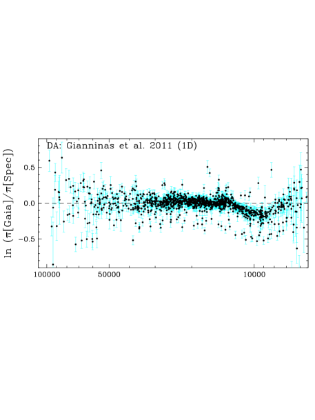
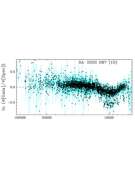
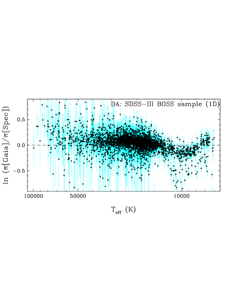
Figure 2: Natural logarithm of the ratio between observed Gaia DR2 and predicted spectroscopic parallaxes for the same samples as in Fig. 1 but with 1D model atmospheres.

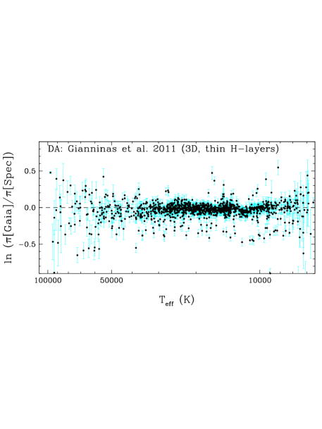
Figure 3: Natural logarithm of the ratio between observed Gaia DR2 and predicted spectroscopic parallaxes using 3D corrections and assuming thin H-layers for the Gianninas et al. (2011) sample.

The comparison of Gaia DR2 parallaxes with predicted values from spectroscopic analyses of DA white dwarfs is presented in Fig. 1 when the atmospheric parameters are corrected for 3D convective effects (Tremblay et al., 2013). The average spread clearly increases going from bright (Gianninas et al., 2011) to faint white dwarfs (SDSS-III BOSS), which is mainly caused by increasing Gaia error bars. Furthermore, the SDSS-III BOSS survey has fewer cool white dwarfs ($T_{\rm eff}<12\,000$ K) owing to a change in the spectroscopic follow-up selection function. Nevertheless there are enough objects over all selected samples to look at systematic trends.

In all three samples, an inflexion is seen in the range between 11 000 K and 13 000 K, where the spectroscopic parallaxes are slightly under luminous. While this is coincident with a high-mass problem (Tremblay et al., 2010), it is also close to the location of the maximum strength of the Balmer lines where $T_{\rm eff}$ determinations are less precise (Bergeron et al., 1995). Fig. 2 demonstrates that when using 1D model atmospheres, there is a strong discrepancy with Gaia for all three samples. This confirms that the 3D model atmospheres, including improved physics, are in much better agreement with the observations (Tremblay et al., 2013). In the range 11 000-13 000 K, it is tempting to suggest that there is a small, residual high-mass problem according to Fig. 1. This is further investigated in Section 4 making use of photometric parameters.

At warm $T_{\rm eff}$ values above 13 000 K where convective flux is negligible, we do not observe a systematic, cross-survey offset between spectroscopic and trigonometric parallaxes. However, both SDSS samples suggest a trend of luminosities that are over-predicted at high temperatures, which is not seen in the Gianninas et al. (2011) sample. One reason could be an issue with our approximate treatment of dereddening (Gentile Fusillo et al., 2018), but this is likely ruled out because the SDSS-III BOSS sample, which covers a larger volume, is not in significantly worse agreement with Gaia. Furthermore, all data sets were analysed with the same models and fitting technique. One explanation for the behaviour is within the spectroscopic calibration of the SDSS spectrograph. It has been reported on many occasions (Kleinman et al., 2004; Tremblay et al., 2011; Tremblay et al., 2016) that SDSS spectroscopic parameters are systematically offset from those of independent surveys but the issue remains unchanged with the DR14 data reduction. However, the SDSS-III BOSS spectrograph with the DR14 data reduction appears to show the same trend. Since both SDSS spectrographs share a data reduction pipeline, it may be that the two SDSS samples are not fully independent and one should be cautious in the interpretation of the differences with the Gianninas et al. (2011) sample.

Fig. 3 demonstrates that if thin instead of thick hydrogen layers are employed for the bright DA stars in Gianninas et al. (2011), the agreement is only marginally worse between spectroscopic and trigonometric parallaxes. It confirms that individual uncertainties are too large to assign hydrogen layer thicknesses on a case-by-case basis (Tremblay et al., 2017; Joyce et al., 2018). Additionally there is no clear split in the Gianninas et al. (2011) distribution of Fig. 1 that would suggest a bimodal distribution of H-layer thicknesses. Whether any information on the mass-radius relation or hydrogen layer masses as a function of white dwarf mass (Romero et al., 2012) can be extracted from these data sets will need to be considered from a more careful statistical analysis with a better understanding of the spectroscopic error bars.

There are a number of outliers in all surveys for which we have carefully examined the data. A significant number of these objects could be DA+DA or DA+DC unresolved double degenerates for which the optical spectrum behaves like a single star. In particular, Figs. 1-2 confirm a fairly obvious sequence of objects at cool $T_{\rm eff}$ below the standard white dwarf sequence where the Gaia fluxes are over-luminous by a factor of about of two, correspond to a parallax offset of a factor 1.5 ($\ln[\pi_{\rm Gaia}/\pi_{\rm Spectro}]\approx-0.35$). These are likely to be unresolved DA+DA double degenerates. DA+DC double degenerates have much more varied spectroscopic solutions owing to the arbitrary dilution of the Balmer lines (Tremblay et al., 2011), and are suspected to be the source of some of the outliers in other parts of the diagram. In some cases, these objects could also be single, helium-rich DA white dwarfs (Gentile Fusillo et al., 2017). Finally, a fraction of outliers are caused by a confusion between the cool and hot spectroscopic solutions (Bergeron et al., 1992), spectroscopic flux calibration issues, or Gaia data issues without raised quality flags. While outside of the scope of this work, this demonstrates the potential of this technique to unravel statistics on the population of double degenerates and helium-rich DA white dwarfs. We note that there are more outliers in the Gianninas et al. (2011) sample than in the SDSS, which is likely because the latter data set includes $ugriz$ photometry and a spectroscopic coverage up to $\approx$ 1 $\mu m$, which allowed us to more easily remove binaries and select between the cool and hot solutions at the pre-analysis stage.

The comparison of the spectroscopic analysis of DB and DBA white dwarfs from Rolland et al. (2018) with Gaia data is shown in Fig. 4 (upper panel). All these objects have a convective atmosphere and Cukanovaite et al. (2018) have recently proposed 3D corrections assuming pure-He composition. Fig. 4 (bottom panel) illustrates the effects of 3D modeling, with the important caveat that this is a preliminary assessment without accounting for the effect of hydrogen on 3D corrections, as the majority of DB white dwarfs are thought to have traces of hydrogen (Koester & Kepler, 2015; Rolland et al., 2018). The parameters of DB stars are in reasonable agreement with Gaia, although for cool objects ($T_{\rm eff}<14\,000~{}$K) where a problem with neutral line broadening is suspected (Rolland et al., 2018), Gaia clearly suggests lower masses than predicted from spectroscopy.

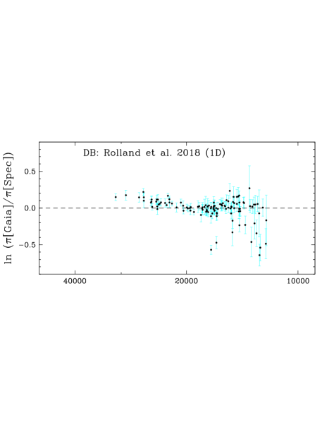
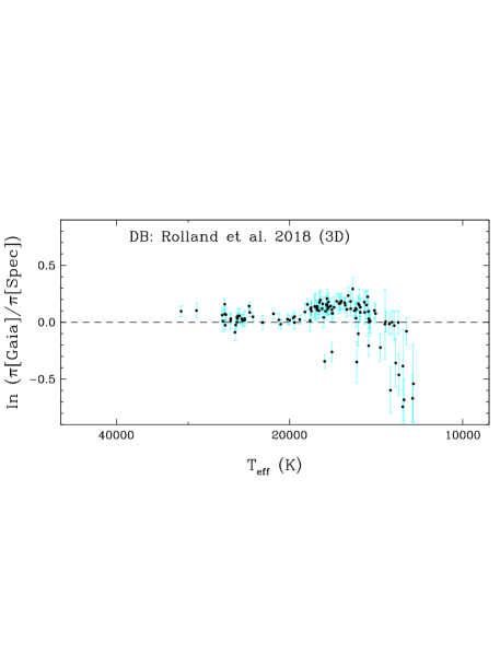
Figure 4: Natural logarithm of the ratio between observed Gaia DR2 and predicted spectroscopic parallaxes for the DB/DBA sample of Rolland et al. (2018) using 1D model atmospheres (Bergeron et al., 2011, top panel) and with 3D corrections (Cukanovaite et al., 2018, bottom panel).

We also present the comparison of Gaia with the SDSS DB and DBA spectroscopic sample of Koester & Kepler (2015) in Fig. 5, once again both for 1D and 3D model atmospheres. For objects below $T_{\rm eff}=16\,000$ K, Koester & Kepler (2015) have assumed $\log g=8.0$ due to potential issues with neutral line broadening. We still show these stars in Fig. 5 but with red points and no error bars. The two published analyses of DB white dwarfs presented in this paper use different models and fitting methods but the agreement with Gaia is similar according to Figs. 4 and 5. For $T_{\rm eff}\gtrapprox 16\,000$ K, both the 3D and 1D atmospheric parameters agree equally well with Gaia within 2$\sigma$ on a star-by-star basis.

The parameters of cool SDSS DB stars where $\log g=8.0$ was assumed do agree with Gaia parallaxes with a very small scatter. This suggests that the mass distribution of DB stars does not have a high-mass problem when the photometric technique is employed, and that the discrepancy is entirely caused by issues with the spectroscopic technique.

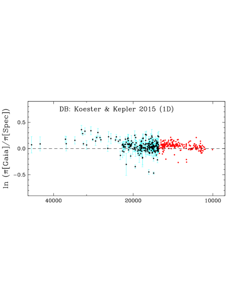
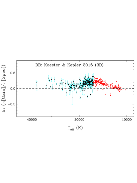
Figure 5: Same as Fig. 4 but for the SDSS DB/DBA sample and model atmosphere fits of Koester & Kepler (2015). Objects with fixed spectroscopic parameters at a value of $\log g=8.0$ are plotted as red points with no error bars.

4 The Temperature and Surface Gravity Scale

The predicted spectroscopic parallax depends on the absolute magnitude which is itself a function of both $T_{\rm eff}$ and $\log g$. As a consequence, it is of interest to study whether both spectroscopic parameters do agree with independent Gaia measurements.

We directly employ the photometric atmospheric parameters derived in section 4 of Gentile Fusillo et al. (2018) and briefly described earlier in Section 2. Gentile Fusillo et al. (2018) have demonstrated that Gaia photometric fits are in very good agreement with fits using instead Pan-STARRS DR1 or SDSS $ugriz$ photometry. As a starting point for this study, we assume that Gaia photometric parameters are as accurate as the model atmospheres, mass-radius relation, and dereddening procedure can describe them. We note that $T_{\rm eff}$ almost only depends on Gaia colours and is degenerate with the fixed dereddening procedure. On the other hand, $\log g$ almost only depends on the absolute Gaia fluxes and is degenerate with the fixed mass-radius relation.

Figs. 6-8 present the comparison of photometric and 3D spectroscopic parameters for our samples of DA white dwarfs. In all cases we can see similar trends, with the Gaia effective temperatures being systematically smaller than the spectroscopic values for all $T_{\rm eff}$, even though individual stars are in agreement within 1-2$\sigma$. The offset was not observed in Section 3 where photometric $T_{\rm eff}$ values were not employed, which could be suggesting an issue with reddening. However, the fact that similar trends are seen for all three samples covering very different volumes suggests that reddening is not the obvious culprit, and we have verified that unrealistic large reddening, i.e. close to the full line-of-sight independently of the distance, is needed to make the temperature scales in agreement. We conclude that a slight issue with the spectroscopic temperature scale is a more likely explanation. The discrepancy is slightly more important for the SDSS spectrograph, suggesting once again an issue with the flux calibration for observations taken up to DR7. The comparison of $\log g$ values has less obvious trends since most objects concentrate around $\log g=8.0$, although there is a slight systematic offset that largely cancels out with the temperature offset when calculating absolute magnitudes, which explains the good agreement in Section 3. It is interesting to remark that when non-ideal effects were included in currently employed Stark broadening tables (Tremblay & Bergeron, 2009), both $\log g$ and $T_{\rm eff}$ changed in the same direction so that the predicted absolute magnitude remained largely constant. Therefore, it is tantalizing to suggest that Gaia may be observing some residual issues in the line broadening. A similar result was found in Genest-Beaulieu & Bergeron (2014) where they used SDSS photometry.

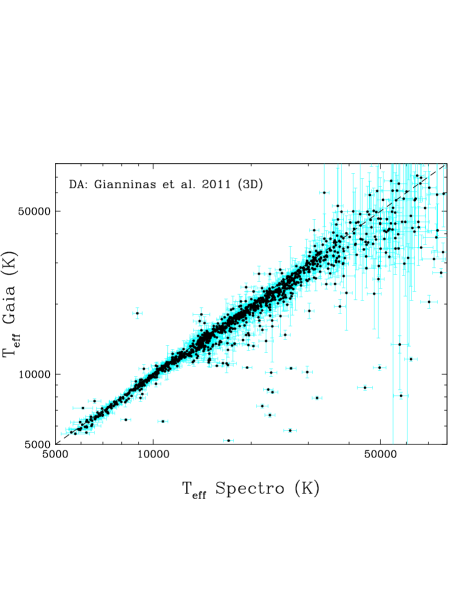
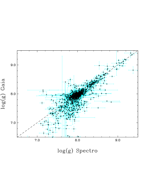
Figure 6: Comparison of spectroscopic and photometric Gaia effective temperatures (top panel) and surface gravities (bottom panel) for the DA sample of Gianninas et al. (2011) corrected for 3D effects (Tremblay et al., 2013). The one-to-one agreement is illustrated by the dashed lines.

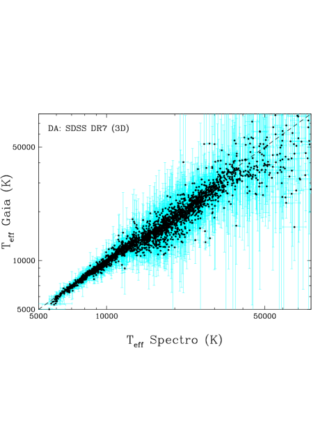
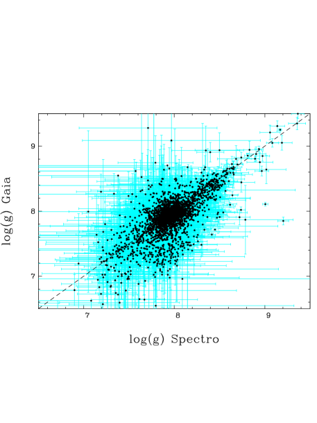
Figure 7: Same as Fig. 6 but for the SDSS DR7 sample.

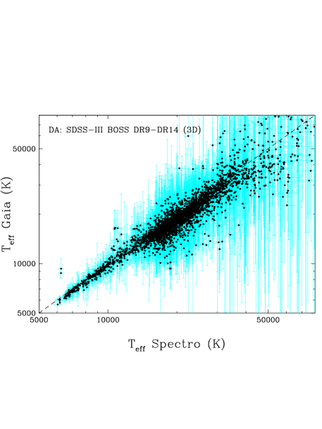
Figure 8: Same as Fig. 6 but for the SDSS-III BOSS sample.

Figs. 9-10 highlight the ratio between photometric and spectroscopic parameters in the region where 3D effects are important for the Gianninas et al. (2011) sample. We employ units of $T_{\rm eff}^{2}$ and $R$, the latter directly derived from the surface gravity because we assume a mass-radius relation, as they are directly proportional to the predicted parallax (Section 3). It is seen that 3D corrections mostly impact the predicted radii, and that there remains a small residual bump around 12 000 K when comparing with Gaia, in agreement with the inflexion observed at the same temperature in Section 3 for the predicted parallaxes. It is interesting to note that Tremblay et al. (2013) had already noticed a small residual bump, with an amplitude of $\approx$ 6%, in the 3D mass distribution of the Gianninas et al. (2011) sample in the range between 11 000 K and 12 000 K. This is consistent with a slight residual high-mass problem that is not fully accounted by 3D $\log g$ corrections in that range. Finally, Fig. 10 confirms a tight sequence of white dwarfs where Gaia suggests that the radius is larger by a factor of about two, or in other words that there are actually two DA white dwarfs at the observed location with similar $T_{\rm eff}$ and $\log g$.

Figure 9: Natural logarithm of the $T_{\rm eff}^{2}$ ratio between Gaia photometric fits and Gianninas et al. (2011) spectroscopic parameters as a function of effective temperature for both 1D (top panel) and 3D model atmospheres (bottom panel).

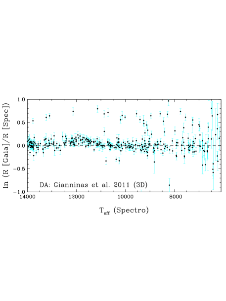
Figure 10: Similar to Fig. 9 but for the radius ratio.

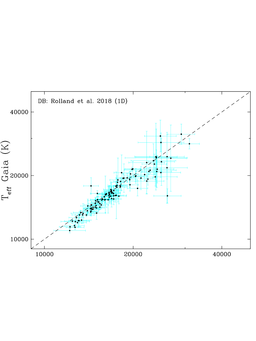
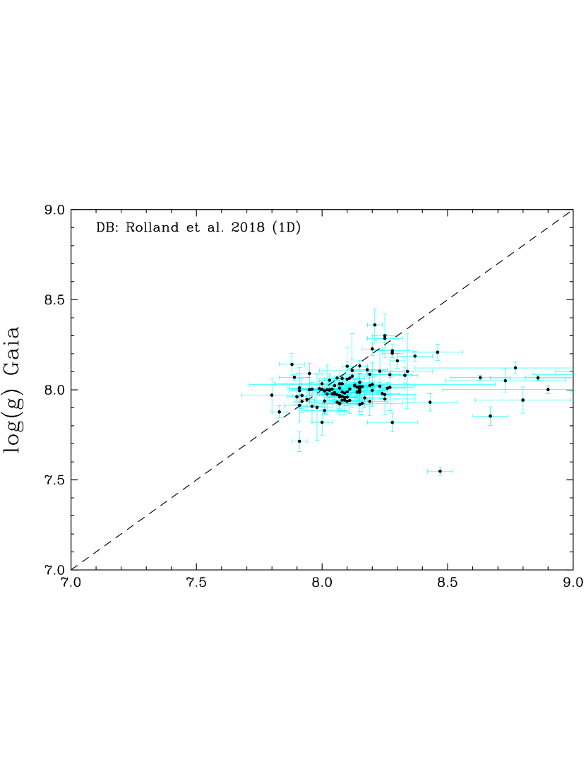
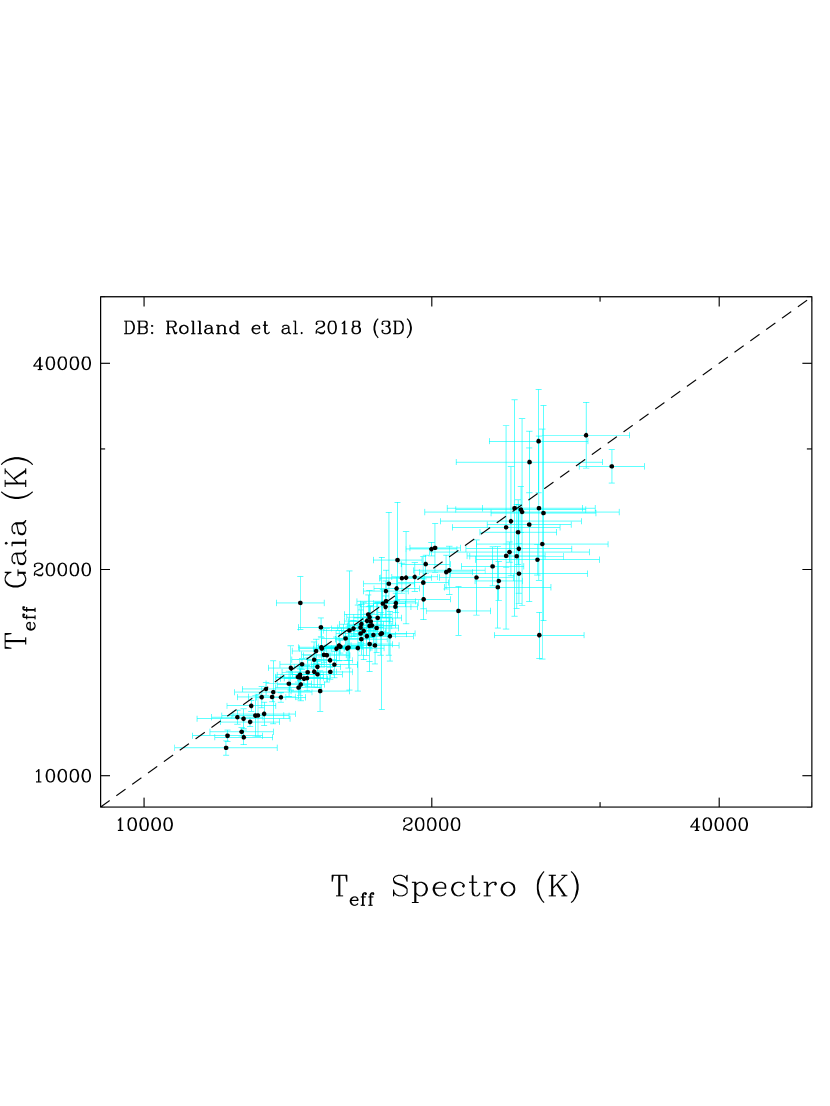
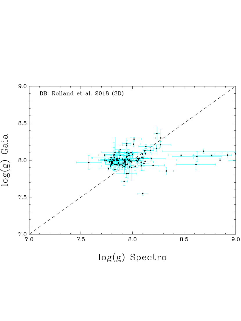
Figure 11: Top panels: Comparison of spectroscopic and photometric Gaia $T_{\rm eff}$ values (left panel) and surface gravities (right panels) for the DB and DBA sample of Rolland et al. (2018). The one-to-one agreement between the two measurements is indicated by the dashed lines. Bottom panels: Similar to the top panels but with the 3D spectroscopic parameter corrections of Cukanovaite et al. (2018) assuming pure-helium atmospheres.

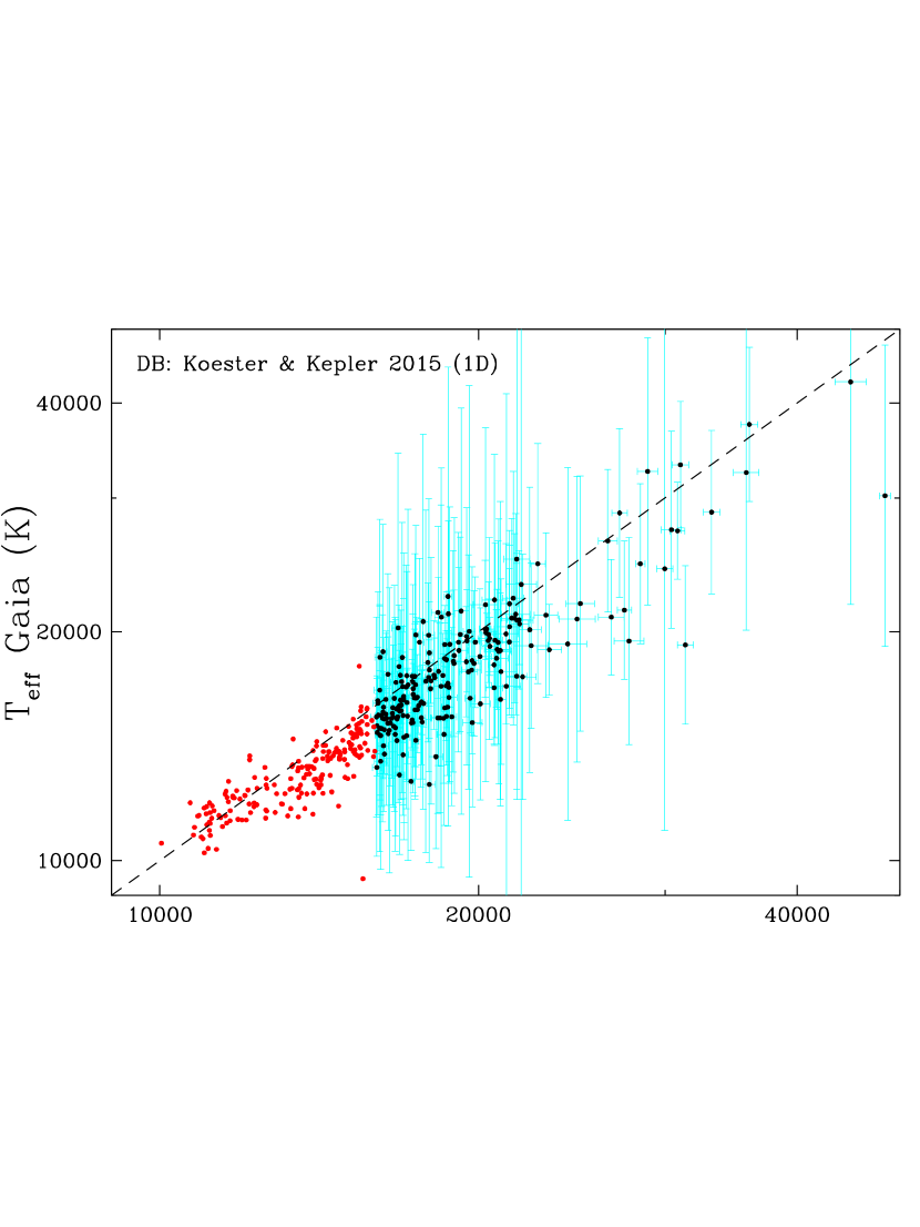
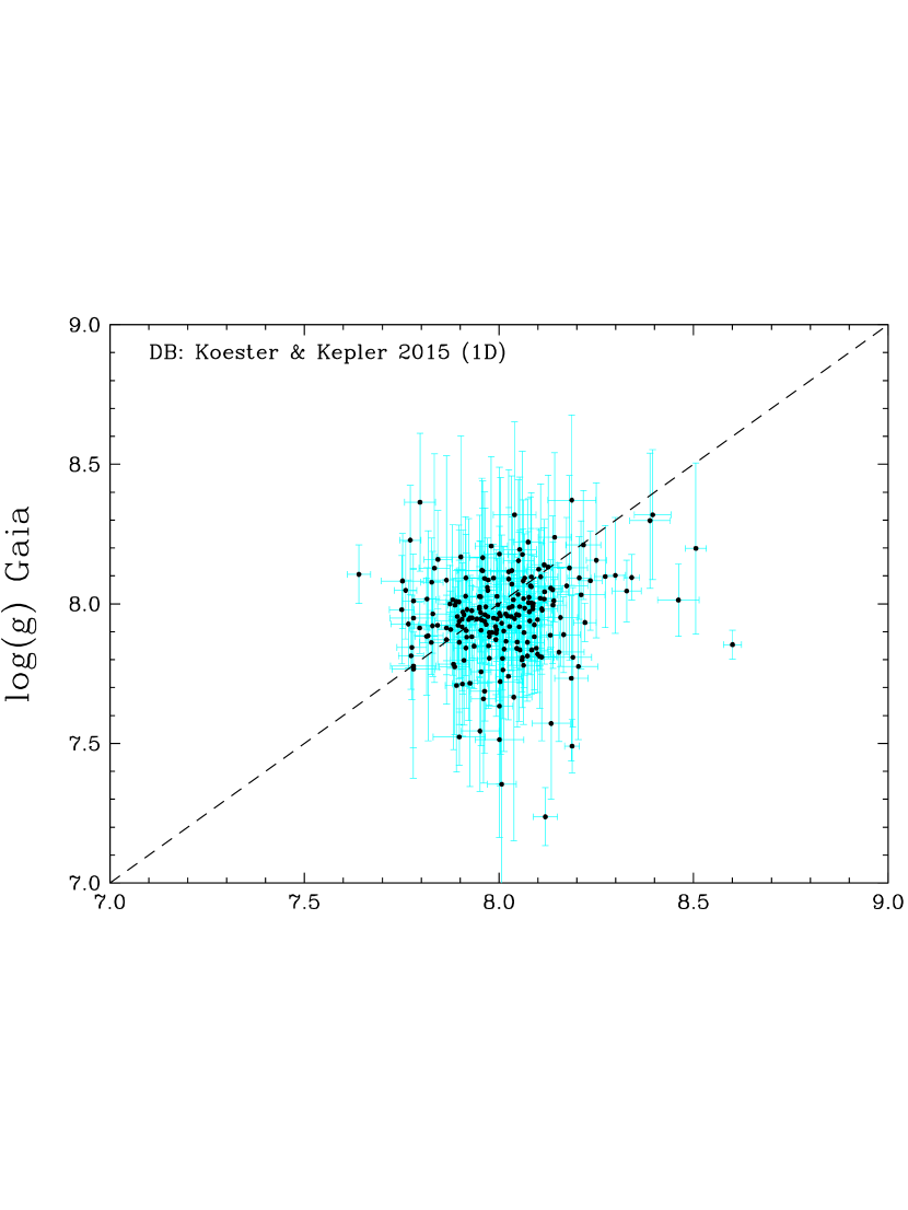
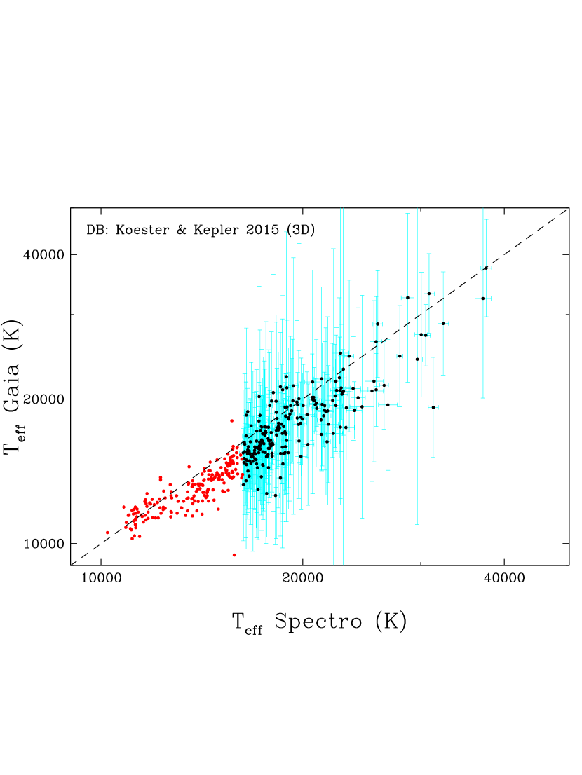
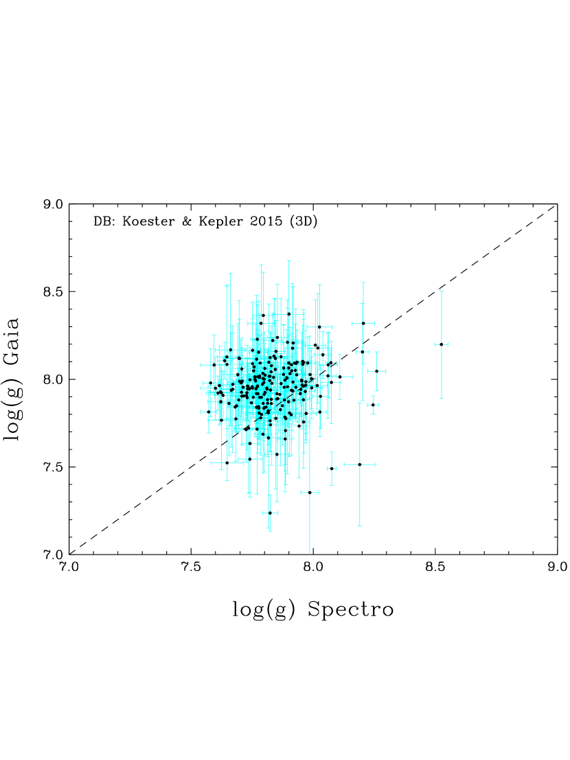
Figure 12: Similar to Fig. 11 but for the DB/DBA sample of Koester & Kepler (2015). Objects with fixed spectroscopic parameters at a value of $\log g=8.0$ are plotted as red points with no error bars on the left panels and omitted from the comparison of $\log g$ values.

The comparisons of Gaia photometric parameters with the DB/DBA spectroscopic samples of Rolland et al. (2018) and Koester & Kepler (2015) are presented in Figs. 11-12. We observe a pattern similar to that seen for DA white dwarfs, with Gaia $T_{\rm eff}$ values being systematically smaller than the spectroscopic ones, both for 1D and 3D models. There is no evidence, however, that the cause is the same as that for DA stars. As it was observed in Section 3, the 3D corrections of Cukanovaite et al. (2018), assuming pure-helium atmospheres, have a significant effect and must be included in the comparison, although they do not bring the spectroscopic parameters into obviously better agreement with Gaia. This must be re-assessed once 3D corrections for DBA stars become available. Finally, we note that all large spectroscopic $\log g$ values in the Rolland et al. (2018) sample, which correspond to objects with $T_{\rm eff}<14\,000$ K, are disproved by Gaia, suggesting instead standard $\log g=8.0$ values for these stars. The discrepancy is not observed in the Koester & Kepler (2015) sample, as they artificially fixed the surface gravity to $\log g=8.0$ for objects with $T_{\rm eff}<16\,000$ K and these stars are not shown on the right panel of Fig. 12.

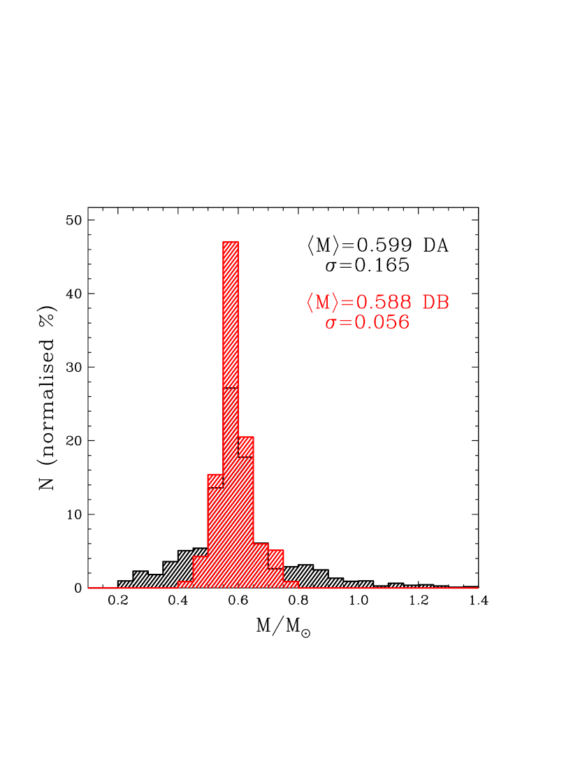
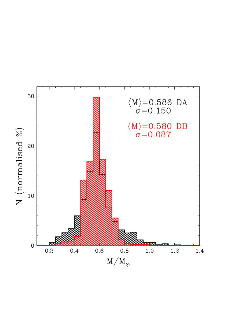
Figure 13: Left: Gaia photometric mass distributions for the DA white dwarfs in Gianninas et al. (2011) and the DB and DBA stars in Rolland et al. (2018). The total numbers of white dwarfs have been renormalised to unity for an easier comparison of the different samples. Right: Similar to the left panel but for the DA white dwarfs in SDSS DR7 and the DB/DBA stars from SDSS DR12 (Koester & Kepler, 2015).

5 Discussion

Gaia photometric parameters allow the derivation of stellar masses by adopting the white dwarf mass-radius relations described in Section 2. Despite their incompleteness, our adopted samples are expected to present a reasonable picture of the field white dwarf mass distribution for a magnitude limited survey, similarly to what has been done in the pre-Gaia era (see, e.g., Tremblay et al., 2016). Gaia selected samples will be more appropriate in the future to study the astrophysical implications of the white dwarf mass distribution, but such samples currently have very poor spectroscopic completeness beyond 20 pc, leading to potentially erroneous interpretations given the strong colour differences between cool DA and DC white dwarfs (El-Badry et al., 2018; Gentile Fusillo et al., 2018).

Fig. 13 compares the photometric mass distributions of DA and DB white dwarfs from the samples of Gianninas et al. (2011) and Rolland et al. (2018), and those found in the SDSS. We neglect the DA sample from SDSS-III BOSS as the results are very similar to SDSS DR7 and for DB stars we have made no such distinction between the SDSS spectrographs. We remind the reader that the mass distributions in Fig. 13 are independent from spectroscopy apart from the sample selection. We find very similar mean masses for all studied samples, suggesting that there is no strong bias from the selection function.

The SDSS sample of DB white dwarfs clearly has a larger standard deviation around the mean compared to the more local Rolland et al. (2018) sample. It illustrates that observational scatter dominates over intrinsic width for the SDSS sample. This is a remarkable result, illustrating that the standard deviation in DB masses is at least three times smaller than for DA white dwarfs and it is unclear if even Gaia is able to resolve the DB mass distribution. For DA white dwarfs, the standard deviations agree well between samples and also between photometric and spectroscopic analyses (Gianninas et al., 2011; Tremblay et al., 2011), confirming that the mass distribution is well resolved.

Gaia DR2 robustly suggests that the mean mass of DA and DB white dwarfs is the same within the uncertainties in the selection function of the samples and the assumption of thick hydrogen layers for all DA stars. However, there is also clear evidence that the DA and DB mass distributions have different shapes, with a sharp decline of the number of DB white dwarfs both at masses lower and higher than the average. These properties observed by Gaia have been suggested before from spectroscopic analyses (Bergeron et al., 2001; Koester & Kepler, 2015; Rolland et al., 2018), but they are now much more firmly established, with possible systematics from 3D effects and line broadening theories largely removed. This illustrates that while both spectral types may have the same mean mass, it can not be concluded that they originate from the same range of progenitors.

Almost all spectroscopically confirmed non-magnetic white dwarfs (e.g., excluding hot DQs, Dufour et al. 2007a) in the age range where DB stars are found appear to have hydrogen-atmospheres for masses below $\approx$ 0.5 $M_{\odot}$ and above 0.7 $M_{\odot}$. This trend appears to continue for older and cooler remnants according to the Gaia-SDSS catalogue of Gentile Fusillo et al. (2018). The behaviour at low masses is not surprising, as these objects are either low-mass white dwarfs ($M_{\rm WD}\lesssim$ 0.45 $M_{\rm\odot}$) or double degenerates. The former must have been formed through close binary evolution to have evolved in less than a Hubble time, and the samples of eclipsing binaries from Parsons et al. (2017) or the extremely-low-mass (ELM) white dwarfs from Gianninas et al. (2014) exclusively contain hydrogen-atmosphere stellar remnants. Double degenerates with mixed spectral types were likely eliminated from our samples as the optical spectra can identify them, which implies that only rare instances of DB+DB double degenerates may populate the very low-mass tail of the DB mass distribution.

The situation at higher-than-average masses is discussed in Gentile Fusillo et al. (2018), with a strong suggestion from young stellar clusters and Gaia that massive white dwarfs overwhelmingly have thick hydrogen layers (Kalirai et al., 2005) and are not subject to convective dilution or convective mixing (Rolland et al., 2018). Furthermore, the detailed shape of the DA mass distribution above 0.6 $M_{\rm\odot}$ could be explained from features in the initial-to-final-mass relation such as the onset of the second dredge-up (Tremblay et al., 2016; El-Badry et al., 2018). There is no evidence to rule out binary evolution for some of these objects (Toonen et al., 2017), but the latter does not lead to an unique, recognisable feature on the higher-than-average side of the white dwarf mass distribution.

6 Summary

Gaia DR2 has detected about eight times more white dwarfs than previously known (Gentile Fusillo et al., 2018). This allows for a rich variety of astrophysical applications, from constraining the local stellar formation history to the initial-to-final mass relation. As a first step, it is essential to understand the accuracy and systematics when deriving the fundamental parameters of these stellar remnants.

We have used DA and DB white dwarfs with well understood spectroscopic parameters and mass-radius relations, and compared these to Gaia-derived absolute magnitudes and fundamental stellar parameters. We emphasise that for all samples studied in this work (Gianninas et al., 2011; Rolland et al., 2018, as well as the SDSS), individual spectroscopic $T_{\rm eff}$ and $\log g$ values of both DA and DB white dwarfs are generally in good agreement with Gaia within 2$\sigma$ when the assumption of a single star is verified. For a few percent of the objects, Gaia has clearly uncovered previously unsuspected double degenerates, although we made no attempt to fully separate the two populations from the available data because of poorly constrained selection functions.

We confirm that even with the precision of Gaia DR2, it is not possible to robustly test the mass-radius relation or derive the hydrogen layer thickness on a star-by-star basis. We observe no evidence of a bimodal distribution of thin and thick layers, which is expected to be most prominent at large temperatures where a warm and thick hydrogen layer leads to a significant increase in stellar radius (Tremblay et al., 2017). However, these hot white dwarfs are generally distant, resulting in a lower Gaia precision and additional uncertainties from reddening. Furthermore, it is possible that additional scatter owing to the presence of undetected metals and NLTE effects (Gianninas et al., 2010) may hinder the detection of thin H-layers.

The size and precision of the Gaia sample has allowed the detection of small systematic offsets between the spectroscopic and photometric parameters. There is a small residual bump in the spectroscopic $\log g$ distribution of DA white dwarfs in the temperature range from 11 000 to 13 000 K, which is likely related to an incomplete account of 3D effects. For DB white dwarfs in the regime below $T_{\rm eff}<14\,000$ K, we find that the spectroscopic technique fails to get accurate surface gravities as it has long been suspected (Bergeron et al., 2011), and Gaia photometric parameters do not appear to have such issue. This is consistent with a problem with neutral line broadening. For both DA and DB white dwarfs, the photometric and spectroscopic temperature scales appear to have a slight systematic offset, with Gaia systematically predicting slightly cooler temperatures by a few percent. We have no obvious explanation for this offset, but residual issues with line broadening theories in spectral analyses remain a possibility.

The present study suggests that Gaia and current mass-radius relations can be employed to derive precise $T_{\rm eff}$, $\log g$, masses, and radii, which is the first step to link white dwarfs to their progenitors. Gaia has clearly confirmed that DA and DB white dwarfs have the same mean mass within less than two percent. However, it was also found that the DB mass distribution has a significantly smaller intrinsic width around its mean than for DA white dwarfs. The next steps will be to understand the precision of the Gaia photometric parameters for other types of white dwarfs as well as gain a better understanding of the cooling rates, e.g. from stellar remnants in wide binaries or clusters.

Appendix A Gaia-SDSS spectroscopic fits

Table 2: *

SDSSJ name	MJD-plate-fiber	$\pi_{\rm Gaia}$	$\sigma_{\rm\pi~{}Gaia}$	3D $T_{\rm eff}$	$\sigma_{\rm Teff}$	3D $\log g$	$\sigma_{\rm logg}$	$\pi_{\rm spectro}$	$\sigma_{\rm\pi~{}spectro}$	Comment
		[mas]	[mas]	[K]	[K]	[cgs]	[cgs]	[mas]	[mas]
000022.88$-$000635.7	51791-0387-166	2.41460	0.28810	23013	473	7.443	0.064	1.84623	0.12224
000034.06$-$052922.4	54380-2624-261	5.12254	0.17227	20299	148	7.799	0.022	5.23086	0.10821
000034.07$-$010820.0	52203-0685-187	5.68123	0.23765	13006	222	8.025	0.054	5.59269	0.25335
000051.85+272405.3	54452-2824-272	2.17536	0.38865	21961	371	7.946	0.051	2.25211	0.10966
000100.42$-$042742.9	54327-2630-359	2.41227	0.32521	17138	225	7.604	0.041	2.50832	0.09545
Notes: Atmospheric parameters are from Balmer line fitting and objects fitted with models including CNO (Gianninas et al., 2010) are indicated in the Comment column. For objects with multiple spectra, we only kept the spectrum with the highest S/N. This is a portion of the table and the full data is available as Supplementary material (online).

Table 3: *

SDSSJ name	MJD-plate-fiber	$\pi_{\rm Gaia}$	$\sigma_{\rm\pi~{}Gaia}$	3D $T_{\rm eff}$	$\sigma_{\rm Teff}$	3D $\log g$	$\sigma_{\rm logg}$	$\pi_{\rm spectro}$	$\sigma_{\rm\pi~{}spectro}$	Comment
		[mas]	[mas]	[K]	[K]	[cgs]	[cgs]	[mas]	[mas]
000006.75$-$004653.9	56956-7850-0719	4.67747	0.35240	11309	139	8.071	0.052	4.13786	0.19743
000022.87$-$000635.6	56959-7848-0062	2.41460	0.28810	22497	185	7.492	0.025	1.90322	0.04927
000034.09$-$052922.4	56564-7034-0336	5.12254	0.17227	19983	131	7.785	0.020	5.15266	0.09676
000104.05+000355.8	56959-7848-0026	3.53414	0.34839	13126	157	8.100	0.036	3.54205	0.11033
000106.93+082825.5	55863-4534-0466	6.60360	0.30072	7682	62	7.931	0.097	6.88215	0.48615
Notes: Atmospheric parameters are from Balmer line fitting and objects fitted with models including CNO (Gianninas et al., 2010) are indicated in the Comment column. For objects with multiple spectra, we only kept the spectrum with the highest S/N. This is a portion of the table and the full data is available as Supplementary material (online).

References

- Abazajian et al. (2009) Abazajian K. N., et al., 2009, ApJS, 182, 543
- Abolfathi et al. (2018) Abolfathi B., et al., 2018, ApJS, 235, 42
- Ahn et al. (2012) Ahn C. P., et al., 2012, ApJS, 203, 21
- Beauchamp et al. (1999) Beauchamp A., Wesemael F., Bergeron P., Fontaine G., Saffer R. A., Liebert J., Brassard P., 1999, ApJ, 516, 887
- Bédard et al. (2017) Bédard A., Bergeron P., Fontaine G., 2017, ApJ, 848, 11
- Bergeron et al. (1992) Bergeron P., Saffer R. A., Liebert J., 1992, ApJ, 394, 228
- Bergeron et al. (1995) Bergeron P., Wesemael F., Lamontagne R., Fontaine G., Saffer R. A., Allard N. F., 1995, ApJ, 449, 258
- Bergeron et al. (2001) Bergeron P., Leggett S. K., Ruiz M., 2001, ApJS, 133, 413
- Bergeron et al. (2011) Bergeron P., et al., 2011, ApJ, 737, 28
- Blouin et al. (2017) Blouin S., Kowalski P. M., Dufour P., 2017, ApJ, 848, 36
- Bohlin et al. (2014) Bohlin R. C., Gordon K. D., Tremblay P.-E., 2014, PASP, 126, 711
- Carrasco et al. (2014) Carrasco J. M., Catalán S., Jordi C., Tremblay P.-E., Napiwotzki R., Luri X., Robin A. C., Kowalski P. M., 2014, A&A, 565, A11
- Chambers et al. (2016) Chambers K. C., et al., 2016, preprint, (arXiv:1612.05560)
- Cukanovaite et al. (2018) Cukanovaite E., Tremblay P.-E., Freytag B., Ludwig H.-G., Bergeron P., 2018, MNRAS, in press
- Dufour et al. (2005) Dufour P., Bergeron P., Fontaine G., 2005, ApJ, 627, 404
- Dufour et al. (2007a) Dufour P., Liebert J., Fontaine G., Behara N., 2007a, Nature, 450, 522
- Dufour et al. (2007b) Dufour P., et al., 2007b, ApJ, 663, 1291
- El-Badry et al. (2018) El-Badry K., Rix H.-W., Weisz D. R., 2018, ApJ, 860, L17
- Evans et al. (2018) Evans D. W., et al., 2018, A&A, 616, A4
- Finley et al. (1997) Finley D. S., Koester D., Basri G., 1997, ApJ, 488, 375
- Fontaine et al. (2001) Fontaine G., Brassard P., Bergeron P., 2001, PASP, 113, 409
- Gaia Collaboration et al. (2018) Gaia Collaboration et al., 2018, A&A, 616, A1
- Genest-Beaulieu & Bergeron (2014) Genest-Beaulieu C., Bergeron P., 2014, ApJ, 796, 128
- Gentile Fusillo et al. (2017) Gentile Fusillo N. P., Gänsicke B. T., Farihi J., Koester D., Schreiber M. R., Pala A. F., 2017, MNRAS, 468, 971
- Gentile Fusillo et al. (2018) Gentile Fusillo N. P., et al., 2018, preprint, (arXiv:1807.03315)
- Gianninas et al. (2010) Gianninas A., Bergeron P., Dupuis J., Ruiz M. T., 2010, ApJ, 720, 581
- Gianninas et al. (2011) Gianninas A., Bergeron P., Ruiz M. T., 2011, ApJ, 743, 138
- Gianninas et al. (2014) Gianninas A., Dufour P., Kilic M., Brown W. R., Bergeron P., Hermes J. J., 2014, ApJ, 794, 35
- Holberg et al. (2012) Holberg J. B., Oswalt T. D., Barstow M. A., 2012, AJ, 143, 68
- Hollands et al. (2018) Hollands M. A., Tremblay P.-E., Gänsicke B. T., Gentile-Fusillo N. P., Toonen S., 2018, MNRAS, 480, 3942
- Hummer & Mihalas (1988) Hummer D. G., Mihalas D., 1988, ApJ, 331, 794
- Jiménez-Esteban et al. (2018) Jiménez-Esteban F. M., Torres S., Rebassa-Mansergas A., Skorobogatov G., Solano E., Cantero C., Rodrigo C., 2018, MNRAS, 480, 4505
- Joyce et al. (2018) Joyce S. R. G., Barstow M. A., Casewell S. L., Burleigh M. R., Holberg J. B., Bond H. E., 2018, MNRAS, 479, 1612
- Kalirai et al. (2005) Kalirai J. S., Richer H. B., Hansen B. M. S., Reitzel D., Rich R. M., 2005, ApJ, 618, L129
- Kalirai et al. (2014) Kalirai J. S., Marigo P., Tremblay P.-E., 2014, ApJ, 782, 17
- Kepler et al. (2015) Kepler S. O., et al., 2015, MNRAS, 446, 4078
- Kepler et al. (2016) Kepler S. O., et al., 2016, MNRAS, 455, 3413
- Kilic et al. (2018) Kilic M., Bergeron P., Dame K., Hambly N. C., Rowell N., Crawford C. L., 2018, preprint, (arXiv:1810.03536)
- Kleinman et al. (2004) Kleinman S. J., et al., 2004, ApJ, 607, 426
- Kleinman et al. (2013) Kleinman S. J., et al., 2013, ApJS, 204, 5
- Koester & Kepler (2015) Koester D., Kepler S. O., 2015, A&A, 583, A86
- Koester et al. (1979) Koester D., Schulz H., Weidemann V., 1979, A&A, 76, 262
- Koester et al. (2014) Koester D., Gänsicke B. T., Farihi J., 2014, A&A, 566, A34
- Kowalski & Saumon (2006) Kowalski P. M., Saumon D., 2006, ApJ, 651, L137
- McCook & Sion (1999) McCook G. P., Sion E. M., 1999, ApJS, 121, 1
- Parsons et al. (2017) Parsons S. G., et al., 2017, MNRAS, 470, 4473
- Provencal et al. (1998) Provencal J. L., Shipman H. L., Hog E., Thejll P., 1998, ApJ, 494, 759
- Rolland et al. (2018) Rolland B., Bergeron P., Fontaine G., 2018, ApJ, 857, 56
- Romero et al. (2012) Romero A. D., Córsico A. H., Althaus L. G., Kepler S. O., Castanheira B. G., Miller Bertolami M. M., 2012, MNRAS, 420, 1462
- Schlafly & Finkbeiner (2011) Schlafly E. F., Finkbeiner D. P., 2011, ApJ, 737, 103
- Schlegel et al. (1998) Schlegel D. J., Finkbeiner D. P., Davis M., 1998, ApJ, 500, 525
- Serenelli et al. (2001) Serenelli A. M., Althaus L. G., Rohrmann R. D., Benvenuto O. G., 2001, MNRAS, 325, 607
- Toonen et al. (2017) Toonen S., Hollands M., Gänsicke B. T., Boekholt T., 2017, A&A, 602, A16
- Tremblay & Bergeron (2008) Tremblay P.-E., Bergeron P., 2008, ApJ, 672, 1144
- Tremblay & Bergeron (2009) Tremblay P.-E., Bergeron P., 2009, ApJ, 696, 1755
- Tremblay et al. (2010) Tremblay P., Bergeron P., Kalirai J. S., Gianninas A., 2010, ApJ, 712, 1345
- Tremblay et al. (2011) Tremblay P.-E., Bergeron P., Gianninas A., 2011, ApJ, 730, 128
- Tremblay et al. (2013) Tremblay P.-E., Ludwig H.-G., Steffen M., Freytag B., 2013, A&A, 559, A104
- Tremblay et al. (2014) Tremblay P.-E., Kalirai J. S., Soderblom D. R., Cignoni M., Cummings J., 2014, ApJ, 791, 92
- Tremblay et al. (2016) Tremblay P.-E., Cummings J., Kalirai J. S., Gänsicke B. T., Gentile-Fusillo N., Raddi R., 2016, MNRAS, 461, 2100
- Tremblay et al. (2017) Tremblay P.-E., et al., 2017, MNRAS, 465, 2849
- Vauclair et al. (1997) Vauclair G., Schmidt H., Koester D., Allard N., 1997, A&A, 325, 1055
- Voss et al. (2007) Voss B., Koester D., Napiwotzki R., Christlieb N., Reimers D., 2007, A&A, 470, 1079
- Werner (1996) Werner K., 1996, ApJ, 457, L39
- Wood (1995) Wood M. A., 1995, in Koester D., Werner K., eds, Lecture Notes in Physics (Berlin, Springer) Vol. 443, Proceedings of the 9th European Workshop on White Dwarfs. p. 41