Statistical complexity of the quasiperiodical damped systems

Abstract

We consider the concept of statistical complexity to write the quasiperiodical damped systems applying the snapshot attractors. This allows us to understand the behaviour of these dynamical systems by the probability distribution of the time series making a difference between the regular, random and structural complexity on finite measurements. We interpreted the statistical complexity on snapshot attractor and determined it on the quasiperiodical forced pendulum.

Ágnes FÜLÖP
Eötvös University
fulop@caesar.elte.hu

1 Introduction

There is no universal definition of complexity in natural sciences. In the last two decades several complexity measures have been introduced, which contain various aspects of complex systems. We mention some ones as algorithmic complexity (Kolmogorov) [17], amount of information about the optimal predict the future corresponding to the expected past (Crutchfield, Young) [8], (Boffetta, Cencini, Falconi, Vulpiani)[6], complexity of finite sequence (Lempel, Ziv) [22].

An important contribution to this issue due to P. Grassberger [13], he studied the pattern-generation by the dynamics of a system and introduced the effective entropy considering the mixture of order and disorder, regularity and randomness, because the most complex situation is neither the one with highest Shannon information $\mathcal{S}$ (random structure) nor the one with lowest $\mathcal{S}$ (ordered structures).

We negotiate the statistical complexity in this article, which allows a description of a finite measured series to consider more complicated dynamical structures which was published in the article [23] (1995). It was widely used in the chaotic regim [9], biology [32], symbolic sequences[1], pseudorandom bit generator[12], earthquake [24], the number system [11].

The entropy appoints the direction of flow. The complexity determines the inner structure of the dynamical system. The statistical approaches are easier to implement than solving equations of motion and they offer the only way of dealing with otherwise intractable problems.

We study the complexity of the quasiperiodic driven dynamical systems considering the snapshot attractor[30] on the set of points, which are determined by the Poencare section. This object corresponds to a given time moment, which contains the points of the trajectories ensemble. These orbits were initialized in the past and the time dependent behaviour was determined by the same equation of motion.

We determined the numerical approximation of the aperiodic driven pendulum, which reflects the behaviour of complexity on the snapshot attractor. This system shows on-off intermittency[20] near to the axis (L=0), due to the fluctuation of the maximal Lyapunov exponent. The maximal Lyapunov exponent linearly intersects the axis, therefore it can be seen, that the system has scaling behaviour [19].

The structure of the article contains the next parts: In the section 1 we introduce the idea of complexity accordingly the measure of entropy and disequilibrium. We discuss the statistical complexity is extended to generalized complexity considering the Tsallis, Wooters, Renyi entropy and the Kullbac-Shannon, Kullbac-Tsallis, Kulback-Renyi divergency. We explained the quasi periodical motion by snapshot attractor, which disposes the on-off intermittency between chaotic and nonchaotic condition and this system provides the scaling behaviour in the section 2. A numerical approximation of the aperiodic forced system is illustrated by the quasiperiodic driven pendulum comparing the complexity and the dissipation rate, which due to the on-off intermittency.

2 Complexity

We investigate the statistical complexity, which is based on the effective entropy by P. Grassberger[13] and the main idea is published by R. López-Ruiz, H.L. Manchini, X. Calbet (LMC) [23, 25, 3, 7].

The expanded definition of the statistical complexity so called generalized statistical complexity measures were introduced by M.T. Martin, A. Plastino, O.A. Rosso (2006) [26], which apply various kinds of entropy and disequilibrium measure [18].

We use the notation of a measured sequence by the article [10]. The time series of the ensemble is denoted by $y_{1,j},\dots,y_{n,j}$, where $y_{i,j}$ means the measurement of the quantity $y$ at time $t_{i}=t_{0}+i\Delta t$, the time interval $\Delta t>0\in\mathbb{R}$ and $j$ $(1<j<m)$ assigned a number of the trajectory in the ensemble. The unit of the time interval $\Delta t$ equals to a constant in this description. The $\underline{x}^{(n)}$ indicates the trajectory of length $n$ in $\mathbb{R}^{d}$, which means a time series of the measurement. The $k$th point of the orbit of length $n$ in the manifold is written by ${{x}}^{(n)}_{k,j}$, where $(k=1,\dots n)$, and $j$ means the number of trajectory $(j=1,\dots m)$ in the manifold. We will research the sequent of $x_{1,j}^{(n)},x_{2,j}^{(n)},\dots,x_{n,j}^{(n)}$ as a time series over the $j$th trajectory. Let us choose this time development quantity of the ensemble at a given moment $i=t^{\prime}$, then we determine the probability distribution of the ${{x}}^{(n)}_{t^{\prime},j}(j=1,\dots m)$ over the points of the trajectories of the manifold.

We rephrase this notation by the symbolic dynamics, because the concept of complexity is much more universal idea than this question. We distinguish $M$ different value of the measurements. The points of the trajectories of length $n$ ${{x}}^{(n)}_{i,j}$ $(1<i<n)$ $(1<j<m)$ are noted by the symbol $o_{i,j}$, which is chosen from the set $\{1,\dots M\}$. Then the $j$th path of length $n$ in the ensemble corresponds to $O^{(n)}_{j}=(o_{1,j},o_{2,j},\dots o_{n,j})$. A series $O^{(n)}_{j}$ $(1<j<m)$ occurs with probability $P(O^{(n)}_{j})$ along a sequent of length $N$ ($n<N$).

2.1 Statistical complexity

The statistical complexity is well applicable concept characterizing finite measurement sequences with its probability distribution. This allows a statistical approximation of the measured quantities. We apply the basic article [23] to introduce this idea.

We suppose that there are $N$ various symbol series of length $n$ $(o_{1,j},\dots o_{N,j})$ $(j=1,\dots m)$ in the ensemble, then these series dispose the set of discrete probability distribution $P\equiv\{p_{1,j},\dots p_{N,j}\}$, where $p_{i,j}:=P(o_{i,j})$ $(\sum_{i=1}^{N}p_{i,j}=1)$ $(1\leq j\leq m)$ and $p_{i,j}>0$ for all $i$.

The statistical complexity measures contains two compositions: (i) entropy $\mathcal{H}$ and (ii) disequilibrium $\mathcal{D}$ i.e. distances in probability-space. It is introduced by the information theory, where the Shannon entropy assigns the gain of the information storage and the disequilibrium features the distance from uniform distribution. So the LMC measure gives a simultaneous quantification of randomness and correlation structures in the systems.

2.1.1 Measure of Entropy and Disequilibrium

Information measure

Information measure $\mathcal{I}[P]$ i.e. the uncertainty can be described by the probability distribution $P=\{p_{j},j=1,\dots,N\}$, with $N$ the number of possible states of the system ($\sum_{j=1}^{N}p_{j}=1$). In the information theory we define the quantity of disorder $\mathcal{H}$ for a given probability distribution $P$ corresponding to the information measure $\mathcal{I}[P]$ in the next term:

$$\mathcal{S}[P]=\mathcal{I}[P]/\mathcal{I}_{max}[P_{e}],$$ (1)

where $0\leq\mathcal{H}\leq 1$, $\mathcal{I}_{max}$ means the maximal value of $\mathcal{I}$, and $P_{e}$ is the uniform probability distribution. Let us consider the Shannon-Kinchin paradigm then $\mathcal{I}$ can be defined as a term of entropies. The statistical complexity was introduced by the Shannon entropy [33], therefore we will investigate this form in a finite system:

$$\mathcal{S}=-\sum_{i=1}^{N}p_{i}\log p_{i}.$$ (2)

This quantity approximately equals to zero $\mathcal{S}\sim 0$, if the symbol sequence $O^{(n)}_{j_{c}}$ has a high probability ($p_{c}\sim 1$) and other $O^{(n)}_{j}$ has very small probability ($p_{c}\sim 0$). In the range of entropy the maximal values $\mathcal{S}_{max}$ corresponds to the uniform probability distribution $p_{e}=\{1/N,1/N,\dots 1/N\}$, which means the the equal probability symbol sequence $O_{j_{e}}^{(n)}$, which leads to the maximum value of information. The normalized quantity ${\mathcal{H}}$ derives from ${\mathcal{H}}=\mathcal{S}/\mathcal{S}_{max}$, than $0\leq{\mathcal{H}}\leq 1$, where $\mathcal{S}_{max}=\log N$.

Disequilibrium measure

We introduce the function of disequilibrium $\mathcal{D}$ on the probability distribution $\{p_{j}:j=1\dots N\}$. The LMC uses some distance $\mathcal{D}$ of a given $P$ compared to the uniform distribution $P_{e}$ in the states of the system [23]. Therefore we investigate the disequilibrium by a distance-form:

$$\mathcal{Q}[P]=\mathcal{Q}_{0}\cdot\mathcal{D}[P,P_{e}],$$ (3)

where $\mathcal{Q}_{0}$ is a normalization constant $(0\leq\mathcal{Q}_{0}\leq 1)$, which equals to the inverse of the maximum possible value of the distance $\mathcal{D}[P,P_{e}]$. The maximum distance is obtained, when one of the components of $P$ i.e. $p_{l}$ equals to one and the remaining elements equal to zero. The disequilibrium $\mathcal{Q}$ differs from zero, if there exist preferred states among the accessible ones, i.e. this quantity features the systems’ architecture.

In the original definition of the statistical complexity the Euclidean norm ($\mathbb{R}^{N}$) have been used i.e. the quadratic distances from the probability distribution of each symbol sequences $P(O^{(n)}_{j})$ $(1\leq j\leq m)$ to the equal probability $P(O^{(n)}_{j_{e}})$. This choice for the distance $\mathcal{D}$ is written:

$$\mathcal{D}[P,P_{e}]=\sum_{i=1}^{N}\left(p_{i}-p_{e}\right)^{2},\;\;\mbox{where}\;\;p_{e}=\frac{1}{N}.$$ (4)

In the range of this quantity becomes maximum, when the disequilibrium achieves prevalent symbol sequences $O^{(n)}_{j_{c}}$ with $p_{c}\sim 1$ and $\mathcal{D}_{c}\to 1$ for $N$ is growing. Otherwise the disequilibrium equals to zero approximately $\mathcal{D}\sim 0$ for $p_{i}\sim 1/N$. The value of the $\mathcal{D}$ changes between these extrema corresponding to advanced probability distribution. The normalized factor equals to $\mathcal{Q}_{0}=\frac{N}{N-1}$.

2.1.2 Measure of statistical complexity

The whole complexity concept includes the functional product of disorder ${\mathcal{H}}$ and disequilibrium $\mathcal{D}$, which based on the various probability distribution corresponding to sequent of the advanced quantity. This shows the transition between the information stored in the system and its disequilibrium. The statistical complexity $\mathcal{C}$ is introduced by the published article of LMC [23]:

$$\mathcal{C}={\mathcal{H}}\cdot\mathcal{D}=-\left(\sum_{i=1}^{N}p_{i}\log p_{i}\right)\left(\sum_{i=1}^{N}\left(p_{i}-\frac{1}{N}\right)^{2}\right).$$ (5)

The value $\mathcal{C}\in\mathbb{R}^{+}$. The normalized $\mathcal{C}$ can be described as follows $\overline{\mathcal{C}}=\overline{\mathcal{H}}\cdot\overline{\mathcal{D}}=(\mathcal{H}/\log N)(\mathcal{D}\cdot(N/(N-1)))$. The range of complexity measure is finite and limiting between $\mathcal{C}_{min}$ and $\mathcal{C}_{max}$, but $\mathcal{H}$ is not necessarily a unique function.

We applied finite system, therefore the statistical complexity disposes the scaling behaviour. A new set of symbol sequences $O^{(n)}_{j}$ turns out at each scale of measurement, which provides an advanced probability distribution $P(O^{(n)}_{j})$ so the value of complexity becomes different.

Three basic cases are distinguished of the statistical complexity: (a) this is monotonous increasing in the function of entropy (b) it corresponds to a convex function, which contains a maximal $\mathcal{C}_{max}$ at the probability distribution $p_{e}$ and the minimum $\mathcal{C}_{min}$ appears, where the ${\mathcal{H}}=0$ i.e. total order and ${\mathcal{H}}=1$ and third kind is (c) the monotonous decreasing with increasing entropy [26].

There are two extremist situations of complexity $\mathcal{C}$ depending on entropy $\mathcal{H}$. On the one hand each set of series assigned to each set of symbol sequence $O^{(n)}_{j}$, which has the same probability distribution. All of them contribute to the information stored in equal measure as the ideal gas [21]. On the other hand, If we study an object, which features some symmetries properties and distance, then this system can be written by minimal information as mineral or symmetry in quantum mechanics.

2.1.3 Generalized statistical complexity

Generalized entropy

We expend the concept of classical statistical complexity to different measures of the entropy and disequilibrium. Tsallis introduced a generalisation of the Shannon-Boltzmann-Gibbs entropic measure [35]:

$$\mathcal{S}_{q}^{(T)}[P]=\frac{1}{(q-1)}\sum_{j=1}^{N}\left[p_{j}-(p_{j})^{q}\right],$$ (6)

where $q$ real number. Renyi suggested a definition of entropy for discrete probability distribution in 1950s years [28]:

$$\mathcal{S}_{q}^{(R)}[P]=\frac{1}{(1-q)}\ln\left\{\sum_{j=1}^{N}(p_{j})^{q}\right\}.$$ (7)

Then the generalized entropy $\mathcal{S}_{q}^{(\kappa)}$ denotes $\kappa=S,T,R$ Shannon,Tsallis and Renyi entropy.

$$\mathcal{H}_{q}^{(\kappa)}[P]=\mathcal{S}_{q}^{(\kappa)}[P]/\mathcal{S}_{max}^{(\kappa)},$$ (8)

where $\mathcal{S}_{max}^{(\kappa)}$ means the maximum value of the information measure, which corresponds the uniform probability distribution. The maximal value of Shannon and Renyi entropy correspond to $\mathcal{S}_{max}^{(S)}=\mathcal{S}_{max}^{(R)}=\ln N$ and Tsallis entropy involves $\mathcal{S}_{max}^{(T)}=\frac{1-N^{1-q}}{q-1}$ for $q\in(0,1)\cup(1,\infty)$.

Generalized disequilibrium

The Euclidean distances was investigated in the LMC. We introduce the generalized disequilibrium $\mathcal{D}$. The Wootters distance was applied for two probability distributions [36], which can be used in the quantum mechanic:

$$\mathcal{D}_{W}[P_{1},p_{2}]=\cos^{-1}\left\{\sum_{j=1}^{N}(p_{j}^{(1)})^{1/2}(p_{j}^{(2)})^{1/2}\right\}.$$ (9)

Consider two divergence-classes, which were published by Basseville [4]. The first class contains the divergence which is defined by the relative entropies. The second class consists of the divergence, which was introduced as the difference of the entropies. The Kullbac-Shannon expression following

$$\mathcal{D}_{\mathcal{K}^{S}}[P,P_{e}]=\mathcal{K}^{(\mathcal{S})}[P|P_{e}]=\mathcal{S}_{1}^{(\mathcal{S})}[P_{e}]-\mathcal{S}_{1}^{(\mathcal{S})}[P].$$ (10)

The Kullback-Tsallis entropy is introduced:

$$\mathcal{D}_{\mathcal{K}^{T}_{q}}[P,P_{e}]=\mathcal{K}_{q}^{(T)}[P|P_{e}]=N^{q-1}(\mathcal{S}_{q}^{(T)}[P_{e}]-\mathcal{S}_{q}^{(T)}[P]).$$ (11)

The Kulback-Renyi etropy following

$$\mathcal{D}_{\mathcal{K}^{R}_{q}}[P,P_{e}]=\mathcal{K}_{q}^{(R)}[P|P_{e}]=(\mathcal{S}_{q}^{(R)}[P_{e}]-\mathcal{S}_{q}^{(R)}[P]).$$ (12)

Then the generalized disequilibrium denoted by this form:

$$\mathcal{Q}_{q}^{(\nu)}[P]=\mathcal{Q}_{0}^{(\nu)}\mathcal{D}_{\nu}[P,P_{e}],$$ (13)

where $\nu=E,W,K,K_{q}$ and $\mathcal{Q}_{0}^{(\nu)}$ normalization constant ($0\leq\mathcal{Q}_{q}^{(\nu)}\leq 1$), and these are:

$$\begin{array}[]{ll}\mathcal{Q}_{0}^{(E)}=\frac{N}{N-1},&\mathcal{Q}_{0}^{(W)}=1/\cos^{-1}\left\{\left(\frac{1}{N}\right)^{1/2}\right\},\\ \mathcal{Q}_{0}^{\mathcal{K}_{q}^{R}}=\frac{1}{\ln N}&\mathcal{Q}_{0}^{\mathcal{K}_{q}^{T}}=\frac{q-1}{N^{(q-1)}-1}.\end{array}$$

Generalized statistical complexity

This quantity is defined following

$$\mathcal{C}_{\nu,q}^{(K)}[P]=\mathcal{Q}_{q}^{(\nu)}[P]\cdot\mathcal{H}_{q}^{(K)}[P],$$ (14)

where $K=S,R,T$ for fixed $q$ and the index $\nu=E,W,K_{q}$ means the disequilibrium with appropriated distance measures. This term (14) is a family of the statistical complexity corresponding to functional product form $\mathcal{C}=\mathcal{H}\cdot\mathcal{Q}$. We notice that the entropic difference $\mathcal{S}[P_{1}]-\mathcal{S}[P_{2}]$ does not specify the information gain or divergence, because this quantity is not necessary positive definit. This lead to the Jensen divergence.

Shinner, Davidson and Landsberg (SDL) published a term for the statistical complexity [34], this term is expressed for $\nu=K,K_{q}$:

$$\mathcal{C}_{K_{q}}^{(\kappa)}[P]=(1-\mathcal{H}_{q}^{(\kappa)}[P])\cdot\mathcal{H}_{q}^{(\kappa)}[P].$$ (15)

We get the LMC statistical complexity at $\kappa=S$, $q=1$ so $\mathcal{C}_{LMC}=\mathcal{C}_{K,1}^{(S)}$.

2.2 Time evolution

In statistical physics we study the isolated systems, which are characterized by initial, arbitrary and discrete probability distribution. The uniform distribution $P_{e}$ develops during the evolution towards equilibrium. Then we can research the time evolution of the LMC i.e. $\mathcal{C}$ versus time $t$ graph. Thanks to the second law of thermodynamics the entropy grows monotonically with time ($d\mathcal{H}/dt\geq 0$) in isolated system. Therefore $\mathcal{H}$ behaves as an arrow of time, so we can study the figure of $\mathcal{C}$ versus $\mathcal{H}$ as the time evolution of the LMC, thus the normalised entropy-axis can be substituted by the time-axis. This picture $\mathcal{H}\times\mathcal{C}$ can be utilized to research the changes in the dynamics of a system, which derives from the modulated parameters.

3 Driven system

In both experimental and theoretical physics, periodically excited nonlinear systems play important role. A typical case of these systems is described by this equation:

$$\frac{d^{2}\Theta}{dt^{2}}+\nu\frac{d\Theta}{dt}+\sin\Theta=f(t),$$ (16)

where the damped forcing f(t) is periodic in time, for example:

$$f(t)=K+V\cos(\omega t).$$ (17)

Such equations are used in many cases of physical research, as forced damped pendulum, the Stewart-McCumber model of the current-driven Josephson junction [2] and simple phenomenological model of sliding charge-density waves [5]. The nonlinear dynamical model can be characterized by strange attractor, period doubling cascades, crises, intermittency, fractal basin boundaries etc. These equations are intensively used in low dimensional chaotic dynamics research.

Periodic excitation is extended to examine aperiodic cases, when $f(t)$ is quasiperiodic for example:

$$f(t)=K+V[\cos(\omega_{1}t)+\cos(\omega_{2}t)],$$ (18)

where $\omega_{1}$ and $\omega_{2}$ are the incommensurate frequencies. It appears in the transition from quasiperiodic to chaos inside an electronic Josphson-junction simulator driven by two independent sources [5]. It is applied on the experiments inside an electron-hole plasma in germanium excited by two frequencies quasiperiodic external perturbations they observed stable three frequencies mode locking, and chaos [14, 15].

These are presented with quasiperiodic systems by two incommensurate frequencies. We consider the following quasiperiodically forced damped pendulum[29]:

$$\frac{d^{2}\Theta}{dt^{2}}+\nu\frac{d\Theta}{dt}+\sin\Theta=K+V[\cos(\omega_{1}t)+\cos(\omega_{2}t)],$$ (19)

where $\Theta$ is an angle of pendulum with the vertical axis, $\nu$ is the dissipation rate, $K$ is a constant, $V$ is the forcing amplitude and $\omega_{1}$ and $\omega_{2}$ are the incommensurate frequencies. Let us investigate new variables, $t\to\nu t$ and $\phi=\Theta+\frac{\pi}{2}$. Then the equation (19) becomes:

$$\frac{1}{p}\frac{d^{2}\phi}{dt^{2}}+\frac{d\phi}{dt}-\cos\phi=K+V[\cos(\omega_{1}t)+\cos(\omega_{2}t)],$$ (20)

where $p=\nu^{2}$ is a new parameter, and $\omega_{1}$ and $\omega_{2}$ are rescaled as follows: $\omega_{1}\to\omega_{1}\nu$ and $\omega_{2}\to\omega_{2}\nu$. In the expressions of the dynamical variables $\phi$,$v\equiv\frac{d\phi}{dt}$ and $z\equiv\omega_{2}t$, then we have

$$\left.\begin{array}[]{rcl}\frac{d\phi}{dt}&=&v,\\ \frac{dv}{dt}&=&p\left\{K+V\left[\cos\left(\frac{\omega_{1}}{\omega_{2}}z\right)+\cos z\right]+\cos\phi-v\right\},\\ \frac{dz}{dt}&=&\omega_{2}.\\ \hline\cr\end{array}\right\}$$ (24)

The equation (24) contains rich dynamical behaviour [31]. This system shows a special behaviour in some range of parameter space. Therefore we apply the snapshot attractor, because this structure reflects the properties of a dynamical systems at a given moment.

The dynamic of the quasiperiodic damped pendulum is characterised by the sign of maximal Lyapunov exponent which changes near to the axis (L=0), because this system has finite fluctuation. The Lyapunov exponent becomes to negative, then the system contracts on the nonchaotic side($L\leq 0$). Otherside the Lypunov exponent turns into positive, then the expansion characterizes the dynamical behaviour on the chaotic side ($L\geq 0$). Therefore the collective properties of the orbits can be studied near to the transition. This is a special behaviour of this model which is called on-off intermittency of the snapshot attractor. The trajectories spend stretches of time expanding (leading to nonzero-size snapshot attractor), yet there are also long time during the trajectories experience contraction, resulting extremely small-size of snapshot attractor. Then the time dependent size of snapshot attractor can be written by the dispersion rate [16]:

$$S(t)=\left(\frac{1}{N}\sum_{i=1}^{N}\left\{[\phi_{i}(t)-<\phi(t)>]^{2}+[v_{i}(t)-<v(t)>]^{2}\right\}\right)^{1/2},$$ (25)

where $N$ is the number of points on the snapshot attractor, $[\phi(t),v(t)]$ defines the geometric center of these points at a given time: $<\phi(t)>=\frac{1}{N}\sum_{i=1}^{N}\phi_{i}(t)$ and $<v(t)>=\frac{1}{N}\sum_{i=1}^{N}v_{i}(t)$.

The time averaged size of the snapshot attractor on the chaotic side near to the transition is defined as $<S(t)>=\lim_{T\to\infty}\int_{0}^{T}S(t)dt$ which obeys the following scaling relation:

$$<S(t)>\sim L\sim|p-p_{c}|,$$ (26)

where $p_{c}$ means the $p\geq p_{c}$ ($L\leq 0$) and $p\leq p_{c}$ ($L\geq 0$). This scaling behaviour of the transition to chaos was published in quasiperiodically driven dynamical systems[19] i.e. a route of chaos was investigated, where the largest Lyapunov exponent passes through zero linearly near the transition to chaos. Because the orbits burst out to separate from each others during the expansion time intervals [27], and the trajectories merge all together during the contraction time interval therefore the size of the chaotic snapshot attractor changes widely in time near to the transition in an intermittent fashion. The average size of the snapshot attractor scales linearly with a parameter similarly as the average interval between the bursts also scales linearly with parameter during transition (26).

4 Numerical approximation

In this section we consider the statistical complexity of the quasiperiodic driven systems, which is represented by the aperiodic forced pendulum (19). We calculated the Poencare section ($z=0$) of the time dependent model (24), which contains a snapshot attractor at the parameter values $V=0.55,p=0.6,K=0.8$ $\omega_{1}=(\sqrt{5}-1)/2$, $\omega_{2}=1.0$. The initial values of the orbits are chosen by uniform distribution in a small volume $<<10^{-6}$ in the phase space. We show the predictability of the intermittency between chaotic and nonchaotic regions.

Statistical complexity

We determined the statistical complexity of this system which was introduced by the quantity of information theory, where the entropy and the disequilibrium depend on the probability distribution (Section2.1.2). The snapshot attractor is written by the ensemble of trajectories instead of the long orbit $N^{\prime}$. Therefore we redefine the probability distribution of the manifold at a time instant $t^{\prime}$.

The ensemble of the snapshot attractor contains the $x_{1,j}^{(n)},x_{2,j}^{(n)},\dots,x_{n,j}^{(n)}$ points of the trajectories of length $n$ $(1\leq j\leq m)$. Therefore the $x_{t^{\prime},1}^{(n)},x_{t^{\prime},2}^{(n)},\dots,x_{t^{\prime},m}^{(n)}$ series corresponds to $\{p_{1},p_{2}\dots p_{m}\}$ probability distribution, where $p_{j}:=P(x_{t^{\prime},j}^{(n)})$ ($j=1,\dots m$).

The entropy $\mathcal{H}$, disequilibrium $\mathcal{D}$ and statistical complexity $\mathcal{C}$ can be determined by appropriate measures using the term of LMC complexity (5). The structure of the complexity is plotted in the $\mathcal{C}\times\mathcal{H}\times\mathcal{D}$ space (Figure 3), where parameter $p$ changes between 0 and 1. The behaviour of complexity $\mathcal{C}$ monotone decreasing, so this corresponds to class (c) over the parameter range [0,1]. In a small interval at $p\simeq 0.8$ the shape of complexity formed convex curve (class (b)).

On-off intermittency

The quasiperiodic damped pendulum provides on-off intermittency in a special values of parameter, where Lyapunov exponent has a finite fluctuation around axis of $L=0$ as it was detailed in the section (3). The volume of the snapshot attractor is widely changing near to axis ($L=0$), therefore we applied the dispersion rate $S(t)$ (25), which scales by the maximal Lyapunov exponent (26). The structure of the complexity $\mathcal{C}(p)$ shows local maximums (Figure 2) similarly as the average of the dispersion $<S(t)>$ over the parameter space $p$ (Figure 1). The complexity reflects the behaviour of the pendulum i.e. the on-off intermittency. Then the probability distribution of the snapshot attractor i.e. dispersion of the trajectories’ points in the manifold at a given time instant $t^{\prime}$ shows similar behaviour as the affect of the on-off intermittency.

Figure 1: The $<S(t)>$ depends on parameter $p$ in logarithm scale.

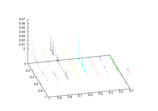
Figure 2: The complexity $\mathcal{C}$ depends on the entropy $\mathcal{S}$ and parameter $p$.

Figure 3: The complexity $\mathcal{C}$ depends on the entropy $\mathcal{H}$ and disequilibrium $\mathcal{D}$ for different parameter $p$ ($0<p<1$).

5 Conclusion

The inner structure of statistical complexity is determined in a quasiperiodical driven system at a given scale. The effect of the on-off intermittency appears in complexity of the aperiodic damped system, which allows the predictability by the by the distribution probabililty of the snapshot attractor.

References

- [1] C. Adami, N.T. Cerf, Physical complexity of symbolic sequences, Physica D 137 (2000) 62-69.
- [2] A. Aiello, A. Barone, G. A. Ovsyannikov, Influence of nonlinear conductance and term on the onset of chaos in Josephson junctions, Phys. Rev. B 30 (1984) 456.
- [3] C. Anteneodo, A.R. Plastino, Some features of the López-Ruiz-Manchini-Calbet (LMC) statistical measure of complexity, Physics Letters A 223 (1996) 348-354.
- [4] M. Basseville, Information: Entropies, Divergences et Mayennes, (IRISA) Publication Interne 1020 (1996) (Campus Universitaire de Beaulieu, 35042 Rennes Cedex, France).
- [5] T. Bhor, P. Bak, M. H. Jensen, Transition to chaos by interaction of resonances in dissipative systems. II. Josephson junctions, charge-density waves, and standard maps, Phys. Rev. A 30 (1984) 1970.
- [6] G. Boffetta, M. Cencini, M. Falcioni, A. Vulpiani, Predictability: a way to characterize complexity, Phys. Reports 356(2002) 367-474.
- [7] X. Calbet, R. López-Ruiz, Tendency towards maximum complexity in a nonequlibrium isolated system, Phys. Rev. E 63 066116.
- [8] J. P. Crutchfield, K. Young, Inferring statistical complexity, Phys. Rev. Lett. 63 (1989) 105.
- [9] G.L. Ferri, F. Pennini, A. Plastino, LMC-complexity and various chaotic regime, Physics Letters A 373 (2009) 2210-2214.
- [10] Á. Fülöp, Estimation of the Kolmogorov entropy in the generalized number system, Annales Univ. Sci. Budap est Sect. Comp. 40 (2013) 245–256.
- [11] Á. Fülöp, Statistical complexity and generalized number system, Acta Univ. Sapientiae, Informatica 6 (2) (2014) 230–251,
- [12] C.M. Gonzalez, H.A Larrondo, O.A. Rosso,Statistical complexity measure of pseudorandom bit generators, Physica A 354 (2005) 281.
- [13] P. Grassberger, Toward a Quantitative Theory of Self-Generated Complexity, Int. Journ. Theor. Phys. 25 (1988) 907–938.
- [14] D.-R. He, W. J. Yeh, Y. H. Kao,Transition from quasiperiodicity to chaos in a Josephson-junction analog, Phys. Rev. B 30 (1984) 172.
- [15] G. A. Held, C. Jeffries, Quasiperiodic Transitions to Chaos of Instabilities in an Electron-Hole Plasma Excited by ac Perturbations at One and at Two Frequencies, Phys. Rev. Lett. 56 (1986) 1183.
- [16] I-A. Khovanov, N-A. Khovanova, P-V-E. McClintock,V-S. Anishchenko, The effect of noise on the strange nonchaotic attractors, Phys. Lett. A 268 (2000) 315-322.
- [17] A.N. Kolmogorov, Entropy per unit time as a metric invariant of automorphism, Doklady of Russian Academy of Sciences, 124 (1959) 754–755.
- [18] A-M. Kowalski, M-T. Martin, A. Plastino, O-A. Rosso, M. Casas, Distances in Probability space and the statistical complexity setup, Entropy 13 (2011) 1055–1075.
- [19] Y-C. Lai, U. Feudel, C. Grebogi, Scaling behaviour of transition to chaos in quasiperiodically driven dynamical systems Phys. Rev. E, 54 (6) (1996) 6070-6073.
- [20] Y-C. Lai, C. Grebogi, Intermingled basins and two-state on-off intermittency, Phys. Rev. E 52 (4) (1995) R3313-R3316.
- [21] P.T. Landsberg, J.S. Shiner, Disorder and complexity in an ideal non-equilibrium Fermi gas, Phys. Lett. A245 (1998) 228.
- [22] A. Lempel, J. Ziv On the complexity of finite sequences, IEEE Trans. Inform Theory 22 (1976) 75–81.
- [23] R. López-Ruiz, H.L. Mancini, X. Calbet, A statistical measure of complexity, Phys. Letters A 209 (1995) 321–326.
- [24] M. Lovallo, V. Lapenna, L. Telesca, Transitionmatrix analysis of earthquake magnitude sequences Chaos,Soliton and Fractals 24 (1) (2005) 33–43.
- [25] M.T. Martin, A. Plastino, O.A. Rosso, Statistical complexity and disequilibrium, Physics Letters A 311 (2003) 126–132.
- [26] M-T. Martin, A. Plastino, O.A. Rosso, Generalized statistical complexity measures: Geometrical and analytical properties, Physica A 369 (2006) 439-462.
- [27] N. Platt, E-A. Spiegel, C. Tresser, On-off intermittency: a mechanism for bursting, Phys. Rev. Lett.70 (3) (1993) 279–282.
- [28] A. Renyi, Probability Theory (North-Holland, Amsterdam, 1970).
- [29] F. J. Romeiras, A. Bondenson, E. Ott, T. M. Antonsen, C. Grebogi, Quasi-Periodically forced dynamic-systems with strange nonchaotic attractors Physica D 26 (1987) 277.
- [30] F.J. Romeiras, C. Grebogi, E. Ott, Multifractal properties of snapshot attractors of random maps, Phys. Rev A 41 (2) (1990) 784–799.
- [31] F-J. Romeiras. E. Ott, Strange nonchaotic attractors of the damped pendulum with quasiperiodic forcing, Phys. Rev. A 35 (10) (1987)4404–4413.
- [32] P.T. Saunders, and M.W. Ho, On the increase in complexity in Evolution II. The relativity of complexity and the principle of minimum increase, Theor. Biol. 90 (1981) 515.
- [33] C.E. Shannon, The Mathematical Theory of Communication, Bell System Technical Journal, 27 (1948) 379-423, 623–656.
- [34] J-S. Shiner, M. Davison, P-T. Landsberg, Simple measure for complexity, Phys. Rev. E 59(2)(1999)1459-1464.
- [35] C. Tsallis, Possible generalization of Boltzmann-Gibbs statistics, J. Stat. Phys. 52 (1988) 479.
- [36] W.K. Wooters, Statistical distance and Hilbert space, Phys. Rev. D 23 (1981) 357.