Uniform Semantics for Interoperability in Engineering Systems Modeling
Abstract
Usually a network of lumped parameter models describes high-level dynamic behavior of a system. Mathematical model of system behaviors is a set of ordinate differential equations or differential algebraic equations. The system integration process hides or encapsulates the geometry of the system. We develop a unified semantics for such models to provide a basis for the standardization and interoperability of system modeling languages. It covers major types of lumped-parameter models and is compatible with other three dimensional models hence connects to geometry. The proposed semantics is based on Tonti diagram. It makes use of cochain complexes, a both geometric and algebraic tool from algebraic topology, as neutral formal syntax. Achieved semantics successfully applied to the interoperation of system modeling languages in single domain. This achievement consolidates the correspondence between algebraic structure and physical system behaviors, provides a possibility for connection to geometry, and therefore sets the stage for automatic design and analysis of engineering systems in computers. It permits model modification, re-utilization and allows direct interpretation of simulation outcomes. Future research will focus on extending the basis for standardization and interoperability of finite element method, discrete and hybrid system modeling languages, economical system modeling languages, etc.
Keywords: Interoperability, Algebraic topology, System modeling languages; Tonti diagrams
1 Introduction
1.1 Motivation
The development of dynamic system is going in the direction of becoming more and more interdisciplinary. Before manufacturing system products, prediction of overall behavior of designed system is particularly significant to avoid unnecessary overhead in time, manpower and material resources. For this reason, there is a desperate requirement of methodologies and theorems on analyzing the integrated interdisciplinary dynamic systems. While analyzing the performance of systems, system behavior plays a key role of describing their state. Description of high-level dynamic behavior of a system usually resorts to a network of lumped parameter models where time is the only independent variable. Languages for creating, editing, and simulating such models proliferated: Bond graphs, linear graph, Modelica, Simullink/Simscape, SysML and graphical interfaces which takes advantage of the graph structure in the network. In principle, all of these languages deal with the same class of problems; but in practice, each is somewhat different in the type of systems, how equations are derived, and how they are simulated. Mathematically seen, the behavior of lumped parameter models is viewed as a set of ordinary different equations (ODEs) or differential algebraic equations (DAEs) whose solutions depend on geometric domain and initial/boundary conditions. However, taking advantage of differential equations to describe continuous physical system shows several shortcomings. It contradicts the fact that every part of an physical system presents and behave simultaneously since differential equations are executed in sequential order. Differential equations are generally expressed by field variables while the geometric representations are associated with global variables that can be directly measured. Using differential equations to integrate discrete entities make the geometry of the system abstracted and encapsulated/hidden.
1.2 Challenges
The proliferation of different and usually incompatible simulation techniques leads to translation problem. Terminology and semantics differs making models incompatible, and complicating exchange, translation, and interoperability of such models. Connection to geometry is lost, making interfacing with 3D simulation tools difficult or impossible. The above challenges can be observed in: (1) recent efforts to incorporate such models of behavior into SysML, but the scope, limitations remain unclear. (2) Functional Mockup Interface - an effort to combine simulation for system integration, but interface systems models to 3D simulations is limited.
proliferation of different and often incompatible techniques
1.3 Contributions
Our aim is to develop a unified semantics for lumped parameter system modeling where geometry, algebra and physics coexist under the same model framework simulating and predicting system behaviors. Geometry represents the configuration, algebra serves as computation tool. It provides basis for the standardization and interoperability of system modeling languages and covers major types of lumped-parameter models. Moreover, the semantics is compatible with other 3D models and therefore make it connects to geometry. The neutral formal syntax of our approach is a tool from algebraic topology, called cochain complexes. Cochain complexes capture the system configuration; combinatorial operations of cochain complexes, a standard algebraic computation tool, describes system behaviors. The ideology of our presentation is based on Tonti diagrams, named after Enzo Tonti, who classified physical variables and equations of classical and relativistic physics into different diagrams. The proposed semantics mainly cover single domain system.
A brief outline of this paper is as follows: in section 2, we survey related works. Section 3 introduces algebraic topological models of physical behavior. Section 4 illustrates modeling process of a single-domain system. The application to express existing languages using proposed semantics is given in Section 5, followed by conclusions and future work in Section 6.
2 Related work
A typical method to describe behavior of dynamic systems is mathematical analysis of lumped-parameter models, such as electrical systems [grandi1997high, massarini1996lumped], mechanical systems [goldfarb1997lumped, parker2000dynamic], thermal systems [mellor1991lumped, gerling2005novel], hydraulic systems [golnaraghi2001development],etc . As the number of lumps increasing, response of models approaches actual system behaviors. Languages for creating such models proliferated in the past fifty years. bond graphs, a port-based modeling of dynamic behavior, initially proposed by H.M.Paynter in 1959, is based on the bilateral relation and its association with the conception of energy [paynter1959hydraulics, paynter1961analysis, karnopp1990system]. The connectivity of physical elements are encapsulated in the junctions. Standardized computer programs have been developed to directly generate system equations from established bond graphs for analysis use. Despite regarded as a universal system modeling language, the geometric information has been abstracted and informationally incomplete [shapiro1989role]. Several years later, linear graph, from mathematical discipline of graph theory, showed its power in physical system modeling depending on intuitive description of element connections. Linear graph uses interconnected line segments to represent lumped parameter system with property of elements allocated to lines. Although linear graph associates topological elements to physical models, it cannot deal with 3D or even higher dimensional models and therefore expanding the number of hierarchy levels of topological elements becomes necessary. [koenig1967analysis, kuo1967linear, blackwell1968mathematical].
In modern time, with the development of computers, people no longer reconciled to manually collect system equations from graphical model thus developed several commercial tools to help engineers efficiently construct system models by taking advantage of physical elements libraries. Simulation afterwards becomes automatic. Simulink is one of such tools. Simulink is a graphical modelling language simulating and analyzing multidomain dynamic systems by signal flow graphs [xue2013system, chaturvedi2009modeling]. It is under a graphical user interface environment. The uni-direction feature of signal flow makes the system running as a one way traffic. Not like other modeling languages based on physical-interaction, numeric information is communication media between physical elements in Simulink. Interaction between two connected elements is realized with the aid of feedback loops. In Simulink environment, Simscape is a system modeling language specially for multidomain physical systems modeling and simulation [esfandiari2014modeling, miller2010real]. Being a powerful complement to Simulink on physical system modeling, Simscape makes use of physical-interaction connections between physical elements. It makes up for the flaw of signal flow on physical modeling - does not subject to conservation laws and cannot intuitively represent the topological structure of systems as a consequence of feedback loops.
Nowadays, aiming to improve modeling efficiency by re-utilization and exchange of models, objected-oriented languages attract engineers’ attention. Modelica is one based on the objected-oriented principle. It is an object-oriented language to model continuous dynamic systems [elmqvist1999modelica, fritzson1998modelica, fritzson2010principles]. The development of Modelica released engineers from using one-to-one corresponding commercial tool to model systems, such as to model electric circuit in spice, multi-body system in Adams, etc. Modelica is powerful on describing system behaviors from heterogeneous engineering domains and allows symbolic manipulation of behavior equations. Even though it has tools connecting to 3D geometry and 3D graphics, necessary graphics properties and interaction between physics and geometry are limited. [engelson20003d].
Currently, with the increasing complexity of large-scale systems, hybrid of systems from multiple disciplines is an inevitable trend, such as engineering system, software system, economical system, etc. System Modeling Language (SysML), as an extension of Uniform Modeling Language (UML), is a graphical language for creating complex and multi-disciplinary system models [friedenthal2014practical, weilkiens2011systems]. Plenty of work has been done exploring the integration of engineering system and simulation. The integration semantics are directly determined by modeling methods of dynamic system behaviors. In SysML, system equations are given in parametric diagrams. But parametric diagrams of SysML and simulation tools are usually not focused on the same type of equations hence intercommunication cannot be directly realized. Another attempt to combine simulation for system integration is the invitation of FMI. This interface provides a standard to generate a uniform model from a given dynamic model. The uniform model can be utilized by other modeling and simulation languages. FMI allows coupled multiple models from different subsystems to be simulated under the same environment by allowing information exchange between them. But it mainly functions in two dimensional simulation, extension to three dimension is still limited.
All the system modeling languages above will be ultimately abstracted to ODEs or DAEs to describe behaviors of physical systems. In contrast, another type of system modeling languages only depend on algebraic equations. It takes advantage of tools in algebraic topology. Indication of correspondence between algebraic structure and physical system behaviors starts from Roth in 1955, four years earlier than bond graph. To describe such correspondence, Roth created his diagram composed of a chain and a cochain. Roth’s diagram focuses on algebraic-topological characterization of one dimensional network problem [roth1955application]. Topological structure of 1-network problems is a linear graph where nodes, branches and loops associate with physical elements of any vector space. The continuity and compatibility of the system hides in a pair reduced homology and cohomology sequences. There is a twisted isomorphism between them representing constitutive laws. Roth’s diagram only considered static and stationary fields, time is not included. In 1977, Branin extends Roth’s diagram to 3-network problems. He replaced the chain and cochain sequences by two cochains [branin2012problem]. Topological structure of 3-network problems contains interconnected points, lines, surface, and volume elements. The appearance of higher dimensional element expands the application of network theory followed by one more constitutive law and four more topological constraints to consider. Branin added time derivatives into the diagram. From Roth’s diagram of electric circuit to Branin’s diagram for electromagnetic field, the role of algebraic topology in network analysis becomes significant.
Tonti used, refined and extended Roth’s and Branin’s diagrams [tonti2003classification]. He classified variables and equations of classical and relativistic physics. The two cochains structure was conserved but time elements are considered. Tonti diagram has front and back double groups of cochains structure. These groups of cochains complexes are connected by time (co)boundary operations hence lead an isomorphism between them. Time derivative is a differential form in Branin’s diagram, but time element of Tonti diagram is an algebraic form by representing time derivative as a coboundary operation on cell complexes of time. For this present paper, the proposed unified semantics of dynamic system modeling is based on Tonti diagram.
3 Algebraic topological models of physical behavior
-
1.
Structure of physical theories a la Tonti
Based on similar types of physical elements and interaction between those elements, physical theories share similar theoretical structure. It is well known as analogies of physical theories. In accordance with this natural tendency of physical theories, the classification of physical variables and equations owns its theoretical foundation. Tonti established such a classification diagram while additionally considering geometric structure associated with physical variables and equations. In order to maintain the geometry of behaviors of physics, he took advantage of cell complexes, an algebraic formulation, as the main computation tool to describe physical behaviors.
-
(a)
classification of the physical variables. [Fig.1]
A system consisting of disconnected physical elements is called primitive system, in which every element functions independently. If global connections are imposed to elements in primitive system, behaviors of independent elements are constrained with each other, then one or several expected behavior occur. Mathematically, variables within physical elements and their mutually connectivity determine system behaviors. Though various types of systems vary widely in terms of behaviors, physical variables in different systems share common classification according to their roles, functions, etc. Tonti classifies physical variables in terms of roles: (1) configuration variables, (2) source variables, (3) energy variables. The definitions of these three variables from [tonti2013mathematical] are cited as follows:
-
i.
configuration variables
Configuration variables describe the configuration of a physical system-variables that linked to a potential by the operations of sum, difference, division by a length, an area, a volume or a time interval; by a limit process and, hence, by time derivatives or space derivatives; or by integrals on lines, surfaces, volumes and time intervals. No physical variables are contained in operations.
-
ii.
source variables
Source variables describe the source of a physical system-variables that linked to them by the operations of sum, difference, division by a length, an area, a volume or an interval; by a limit process and, hence, by time and space derivatives; line, surface, volume and time integrals.No physical variables are contained in operations.
-
iii.
energy variables
Energy variables are defined as the multiplication of a configuration variable by a source variable-variables linked to them, by the operations of sum, difference, division by a length, an area, a volume or an interval; by time or space derivatives; or by integrals on lines, surfaces, volumes and time intervals.
Source variables play a role of stimuli for the system while the configuration variable describe the system ”shape”. Without stimuli, system would stay at the initial state; without system configuration, incentive has no action point. Energy variables, the product of source and configuration variables, specify the distribution of energy of the whole system. Fig.1(a) shows the relations between those variables. The relation of variables within the same class satisfies topological equations - namely, gradient equations, circuital equations and balance equations as shown in Fig.1(b).

(a) elementary unit of diagram 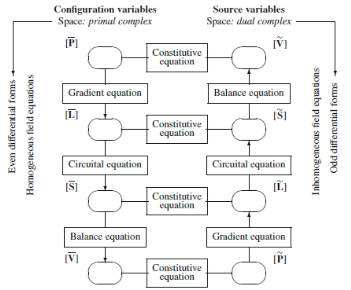
(b) Positions of configuration and source variables in Tonti diagram Figure 1: The classification of the physical variables -
i.
-
(b)
Geometric properties of physical variables
The mathematical machinery representing the physical variables is taking advantage of geometric and algebraic objects. According to the existing form in physical space, every physical variable associates with one geometric element (point/line/surface/volume), such as electric current is associated with a line, temperature is associated with a point. If each geometric element is furthermore allocated algebraic values, the combination of geometry and algebra would become powerful tool in modeling and computation of physical systems. Geometric elements are allocated to both space and time in Tonti’s diagram, named as space and time elements respectively. Space elements determine the field shape of physical systems at a time instant, time elements describe real-time change of field of one geometric configuration.
Since the direction character of physical variables, i.e. direction of fluid flow, allocated geometric elements are expected to own orientation property. Directed geometric elements maintain the original geometric elements characters while providing convenience for algebraic computation afterwards. Tonti defines two orientations (inner and outer) to geometric elements. The criterion to assign orientations of space and time elements is oddness principle, which is defined based on experimental evidence.
Oddness principle: Every global physical variable referring to an oriented space or a time element reverses its sign when the orientation of the space or the time element is reversed
According to the oddness principle, if reversal of space/time-element orientation affects the sign of a variable, the variable is assigned with inner space element /// and inner time interval element or outer time instant element . Otherwise, it is assigned with outer space element /// and outer time interval element or inner time instant element .
-
(c)
Introduction of cell complex
To represent the system state in a mathematical way, a reference structure is a must. Differential formulation takes advantage of coordinate system as reference structure. Algebraic formulation usually takes advantage of ”meshes” as reference structure, for examples, meshes in finite element method. The cell complexes provide us a powerful reference structure that combines both geometric and algebraic tools to model geometry and conduct computation of physical systems. Some necessary terminologies of cell complex for system modeling are introduced below.
In cell complex, -cells () denote the -dimensional geometric elements. A cell complex is an assembly of -cells. In Euclidean space, -cells represent points, lines, surfaces, volume respectively. Orientations of a -cell are compatible with the ordering of the vertices of the cell. This is consistent with the inner orientation defined in Tonti’s diagram. Outer orientation of a -cell inherits from the inner orientation of its dual, a -cell, where n is the dimension of the physical space. If the cell complex consisting of all -cells is called primal cell complex, then the cell complex consisting of all dual of -cells is called dual cell complex. Primal and dual cell complexes are dual to each other so one can call either of them primal and the other dual. Usually in Tonti diagram, primal cell complex consists of p-cells with inner orientation, dual cell complex consists of -cell with outer orientation. Fig.2 shows a pair of primal and dual cell complexes in a three dimensional space.

Figure 2: A cell complexes and its dual in three dimensional space -
(d)
The structure of Tonti diagram
-
i.
The two different structures of Tonti’s diagram in terms of mechanical and field theories.[Fig.3]
Based on the physical nature of sources, physical theories are usually divided into two kinds: (1) mechanical theories - sources are forces (2) field theories - other types of sources. In Tonti diagram, positions of space elements of these two theories are the same but positions differ within time-even elements ( or ) and time-odd elements ( and ). Fig.3 shows classification diagrams of mechanical and field theories, in which physical variables at each circle associates with a pair time and space elements. They are linked to each other by sets of equations: (1) variables on the left and right sides are linked by constitutive equations (2) variables at two adjacent vertical levels are linked by topological equations (3) variables at front and back sides are linked by coboundary operation in terms of time elements.
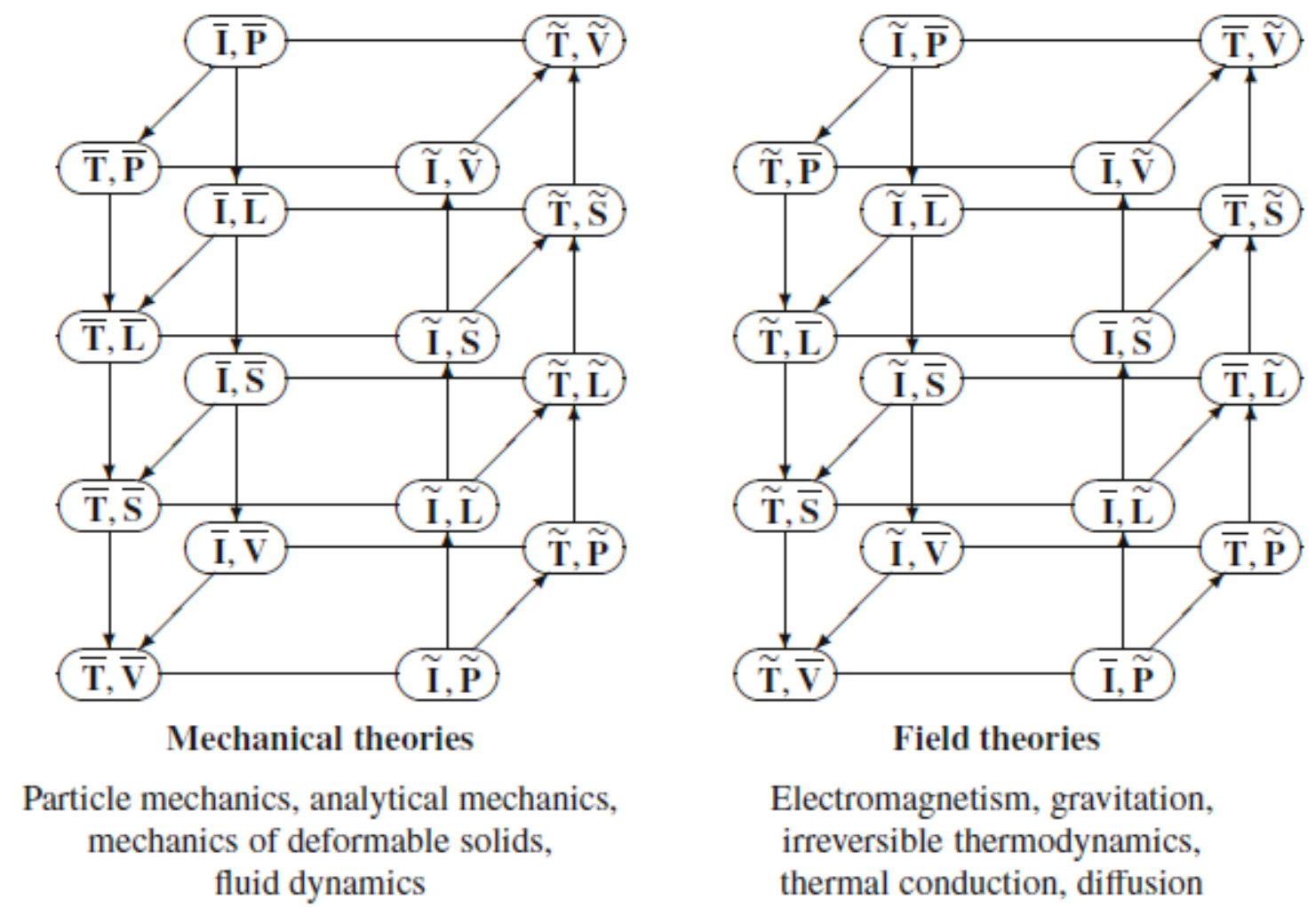
Figure 3: Behavior of field function -
ii.
Single primal-complex formulation is not reasonable, it is necessary to identify primal and dual cell complexes
Unlike other graphic languages of continuous system modeling, such as block diagrams, bond graphs, linear graphs where only one reference structure is sufficient for mathematical computation, Tonti diagram consists of two reference structures, primal and dual cell complexes. Either of them is not redundant because the cells dimension associated with a pair configuration and source variables may not the same thus they can not coexist in the same function space. Furthermore, even though the outer orientation of a dual cell inherits the inner orientation of its primal cell, the vector space embedded by configuration and source variables is independent from orientation inheritance.
-
iii.
balance,circuital,gradient equations (and corresponding dual equations)
Two adjacent vertical levels of Tonti diagram are linked by topological equations which plays a role of constraints in spatial dimensions: (1) gradient equations define the difference of variables associated with two points / (2) circuital equations define a relation between variables associated with faces / and those associated with boundaries / of faces. (3) Balance equations denote the conservation of energy of a system where the amount of variable produced in a domain equal to the amount flowing out of the domain plus the residual. Algebraically seen, topological equations can be expressed by cell complexes and coboundary operations.
-
i.
-
(e)
(co)boundary operations of cell complexes.[Fig.4]
Cell complex is one kind reference structure for algebraic formulation, the mathematical operator of it is boundary and coboundary operators. They are both linear operators. Given a cell complex, a face of a -cell is a -cell incident to the -cell; a coface of a -cell is a -cell incident to the -cell. The boundary operation of a -cell is to obtain all its faces; the coboundary operation of a -cell is to obtain all its cofaces [hatcher2001algebraic]. A group of -cell is named as a -chain having the form:
(1) where is -chain, represent the - cell of -chain, is the number of cells in -chain. denotes the multiplicity. is a finite collection of n simplices with integer multiplicities-the coefficients . The cochain is dual of the chain group . Since p-simplices form a basis for , coefficients of cochains are more general-real numbers, vector spaces,etc. -cochains are equivalent to functions from -simplices to the coefficients group. A -cochain is defined as
(2) where, is -cochain, denotes the general coefficients. The generalization of coefficients extends the functionality of cochains to represent a physical scalar/vector variable associated with a cell.
The boundary operation of a -chain is a collection of all faces of -cells of the -chain. Multiplicity of a face is addition of multiplicities transferred from all adjacent -cells of it. The boundary operation of a -cell with multiplicity is as follows:(3) where, is the number of cells in -chain, denotes the incidence number of a -cell and a -cell : if is not a face of , then ; if relative orientation between and is compatible, then ; if relative orientation between and is incompatible, then . Thus, the boundary operation over a -chain is as follows:
(4) Contrast to boundary operation of chain, the coboundary operation of cochains complex is collecting all cofaces of all -cells of a -cochain. Given a -cell with a multiplicity ,
(5) where, is the number of cells in -chain, denotes the incidence number of -cell and -cell : if is not a coface of then ; if relative orientation between and is compatible, then ; if relative orientation between and is incompatible, then then . The coefficient of a coface, -cell, is addition of coefficients transferred from all adjacent -cells of it.Thus, the coboundary operation of a -chain is as follows:
(6) Since the duality of primal and dual cell complexes, the boundary of a -chain and coboundary of a -cochain have the same form:
(7) where, n is the dimension of space, represents the boundary operation of a -chain in primal cell complex, denotes the coboundary operation of a -cochain in dual cell complex. For example, in a three-dimensional space, if primal 0-cells are oriented as sinks and dual 3-cells are induced with the inward orientation, then .
Because cochains are generated from chains with more general coefficients, chains can be also treated as cochains, coboundary operation of chains is therefore mathematically reasonable. In the following practice, we will view all chains as cochains. The boundary of a -chain and coboundary of a -chain in the same primal cell complex have relation:
(8) In algebraic formulation, three kinds of topological equations in primal cell complex are defined by coboudary operators: -gradient equation, -circuital equation, -divergence equation. The topological equations in dual cell complex are defined by -gradient equation,-circuital equation and -divergence equation. The relation of coboundary operator in primal and dual cell complexes derived from Eq.7 and Eq.8 is as follows:
(9) Classification diagram uses letters , , , to represent the , , as shown in Fig.4. The ”minus” symbol in exists due to the custom of defining outer orientation of a volume in physics, which is reversed to orientation the volume should have inherited from its dual point.
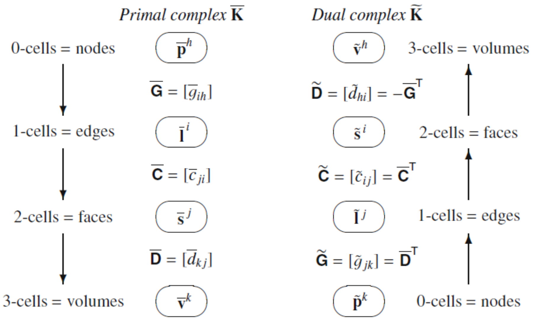
Figure 4: incidence numbers of three dimensional cell complex and its dual In time domain, to obtain variables below using coboundary operations in terms of time, we call it time coboundary operations.
-
i.
mesh charge (displacement)
-
ii.
mesh currents (velocity)
-
iii.
rate of mesh currents (acceleration)
Spacetime combines space and time into a uniform mathematical model of physics to study both non-relativistic and relativistic physical phenomenon. In algebraic formulation, the reference structure of spacetime is four dimensional cell complex: three dimensions represent the spatial region; one dimension represent the time axis. If add one dimensional cell complex of time to primal three dimensional cell complex of space, we obtain a primal four dimensional cell complex of spacetime. If add one dimensional cell complex of time to dual three dimensional cell complex of space, we obtain a dual four dimensional cell complex of spacetime.
Projection of primal and dual cell complex of spacetime to time axis shows us the adjacency of cells and duality of primal and dual cell complex of time as given in Fig.5. The primal cell complex of time are vacuum 0-cells and green 1-cells; the dual of it are solid 0-cells and red 1-cells. Primal/dual time instants (intervals) are associated with primal/dual 0-cells(1-cells) respectively.
The velocity and acceleration of a physical variable can be directly obtained under reference structure of space time and coboundary operation without need to separately discretize time in differential formulation. Take variables from electric network as an example, 0-cochain of mesh charge in primal cell complex is associated to primal time instants; the velocity of it, usually called mesh currents, can be obtained by coboundary of time as follows:
(10) where, is the time interval; donates the time coboundary operation of 0-cochain time instants in primal cell complex. Eq.10 assumes the time axis is divided by the same intervals.
To obtain the rate of mesh currents, we need to use the dual time cell complex. Re-associate the obtained 1-cochain mesh currents to dual time instants where it is re-defined as a 0-form , the acceleration of mesh charge , that is the velocity of mesh current is obtained as follows:
(11) where, , deleting the first and last rows of , is a restricted time coboundary operation of 0-cochain time instants in dual cell complex. It deletes the first and last row of . This is because if there are 5 initial mesh charge, we can only obtain 4 velocities and 3 accelerators of it as shown in Fig.5. Although the dimension of () induces the dimension of (), the effective parts of to deduce the acceleration are rows except the first and last rows.
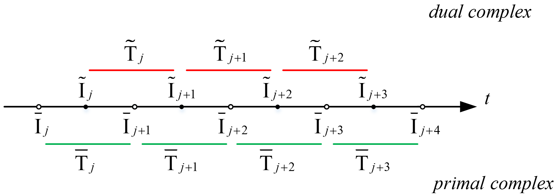
Figure 5: Primal and dual time elements -
i.
-
(f)
Governing equations [ferretti2015cell]
-
i.
grad: algebraic form vs differential form
-
ii.
curl: algebraic form vs differential form
-
iii.
div: algebraic form vs differential form
-
i.
-
(g)
Fundamental equations
Physics equations relating physical variables to express the behavior of physics field and system, are usually divided into five sorts: (1) defining equations - define new variables (2) topological equations - constrain values of variables through boundaries. (3) Equations of behaviors - specify a behavior condition must be obeyed (4) constitutive equations - associate source and configuration variables (5) coupling equations - describe relation of variables of different physical domains. Fundamental equations consist of above five sorts of equations, which turns physical problems to fundamental mathematical problems that describe the real-time configuration and behavior of physical systems. Fundamental equations of the main physical theories can be obtained by following specific paths in Tonti diagram.
-
(h)
Analogies of physical theories. [Fig.6]
Topological structure and physical elements co-determine the behavior of systems which is caused by the exchange, storage, dissipation of energy and physical information of the systems. As Fig.6 shows, in a singular domain physical system, types of physical elements are usually classified into (1) generalized resistors (2) generalized capacitors (3) generalized inductors (4) generalized voltage sources (5) generalized voltage sources [durfee2009fluid]. Although the behaviors of different physical systems with same topological structure are different, the running mechanism of physical elements of the same type are the same. This is the analogies of physical theories.
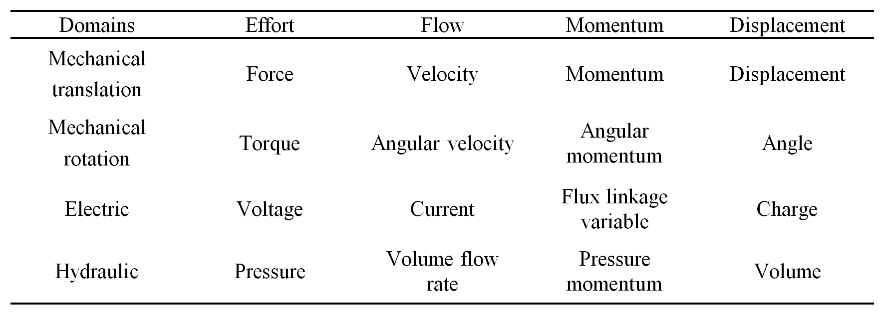
Figure 6: analogy of physical theories
-
(a)
4 Modeling of single-domain lumped parameter system
-
1.
Introduction of lumped parameter system
-
(a)
Definition of lumped parameter system
Mathematically speaking, the lumped parameter, as opposed to distributed-parameter means no spatial derivative, which is a simplification reducing partial differential equations (PDEs) of a physical system model of infinite number of degrees into ordinary differential equations (ODEs) of a finite degrees. The lumped parameter system is a topological structure consisting of discrete entities obtained by simplifying spatially distributed physical systems under specific assumptions [doebelin1998system].
-
(b)
Features of lumped parameter system
Variables of a lumped parameter system are assumed to be uniform in a finite spatial region yet properties of components are complete and self-contained. The analysis of lumped parameter systems stays at the component level. For a lumped parameter system, time is the only independent variable hence common measure to take to describe its behaviors is using ODEs by linking components together. With the birth of Tonti diagram, escpecially the introduction of time elements, pure AEs approximating system behaviors has been realized.
-
(a)
-
2.
Feasibility of modeling lumped parameter system in terms of Tonti diagram
-
(a)
Necessary factors of modeling a lumped parameter system
-
i.
interconnection between components
Each modeling language of continuous systems has its particular methodology to describe the interconnection between components. Bond graph takes advantage of 0 and 1 junctions to describe parallel or serial connection of components; Modelica/Simulink use connectors to link components; Linear graph uses connected lines to show the connectivity. For the Tonti diagram, the interconnection between components is described through the connection of cells and mathematically expressed by the (co)boundary operations. Such interconnection described by (co)boundary operations is more intuitive on describing the topological structure and running mechanism of physical system since it associates each variables of system component with one independent space element.
-
ii.
constitutive equations of components
Besides the interconnection between elements representing the topological structure of systems, the constitutive equation describes the behavior property of elements and functions as the constraints on degrees of behavior freedom. It is a necessary part included in each modeling languages: Bond graph associates across, through and constitutive variables to 1-ports; Modelica/Simulink stores the constitutive equations in the library where components are sorted by type; Linear graph explicitly associates constitutive variables with lines and implicitly associates across, through variables with lines. In Tonti diagram, the dissipative constitutive equations locate at the diagonal of the diagram; conservative constitutive equations locate at horizontal links between configuration and source variables of the same level.
-
i.
-
(b)
Describing system behaviors based on established models
When the model of systems are established, based on the information of connectivity and constitutive equations of elements, systems can be abstracted to mathematical equations, describing the system behaviors. Equations describing system behaviors are usually called state equations which usually consists of a set of DAEs in differential formulations or algebraic equations(AEs) in algebraic formulations. System state equations deduced from Tonti diagrams are AEs.
-
i.
Standard procedure to deduce state equations
Each system modeling language has a standard way to deduce system state equation, the procedure of which are generally introduced as follows:
Bond graph : (1) Assign causality to bond graph (2) select input and energy state variables (3) generate initial set of system equations (4) Simplify initial equations to state-space form [karnopp2012system].
Modelica/Simulink: (1) Based on the established model in Modelica/Matlab, extract equations of each component from library (2) find out dynamic variables which are state variables if DAE reduces to an ODE (3) express the problem as the smallest possible ODE system.
linear graph: (1) generate a normal tree from the linear graph (2) Select the primary and secondary variables, system order, state variables. (3) Formulate constitutive, continuity and compatibility equations and take advantage of these equations to obtain state equations
Tonti diagram: (1) given a physical system, find out the corresponding tonti diagram of this system. (2) follow paths in the diagram to obtain each item in the given fundamental equations (3) Sum up all the items. The fundamental equations given in the diagram are state equations of the system. The dual form of this state equation can be obtained by following the dual of the above paths in the diagram.
-
i.
-
(a)
-
3.
System of single dissipative constitutive relation [bamberg1991course]. [Fig.7]
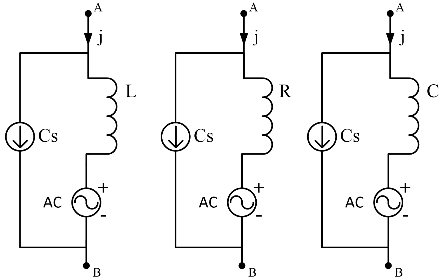
Figure 7: composite branch convention -
(a)
We will first forcus on the simplest linear steady state system where time is not included. Examples in this part are based on electric circuit of pure resistance, examples of pure generalized resistance in other physical systems can be solved in a similar way.
-
(b)
System modeling in terms of Tonti diagram
-
i.
The basic component of the system is shown in Fig.7
As can be seen from Fig.7, the fundamental unit of an physical system of pure resistance is made of a voltage source, a current source and a general resistor, where the polarity of sources can be arbitrary reversed and resistor can solely exist without either or both sources. Refer to [bamberg1991course] for more details. An electric circuit of pure resistance consists of at least one fundamental unit.
-
ii.
Model structure in Tonti diagram
All the information about physical systems model of pure resistance: interconnection of elements and dissipative constitutive equations, are contained in the two cochains linked by the diagonal lines. Specifically, interconnection of components is given by the three topological equations, dissipative constitutive equations are given on diagonal lines. With this modeling structure, system state equations can be obtained in a standard way.
-
i.
-
(c)
System behavior description in terms of Tonti diagram
-
i.
Follow routes in Tonti diagram to obtain state equations
The first method is based on Kirchhoff’s current law, following the primal cycle of diagram [ELE10] as shown in Fig.8.
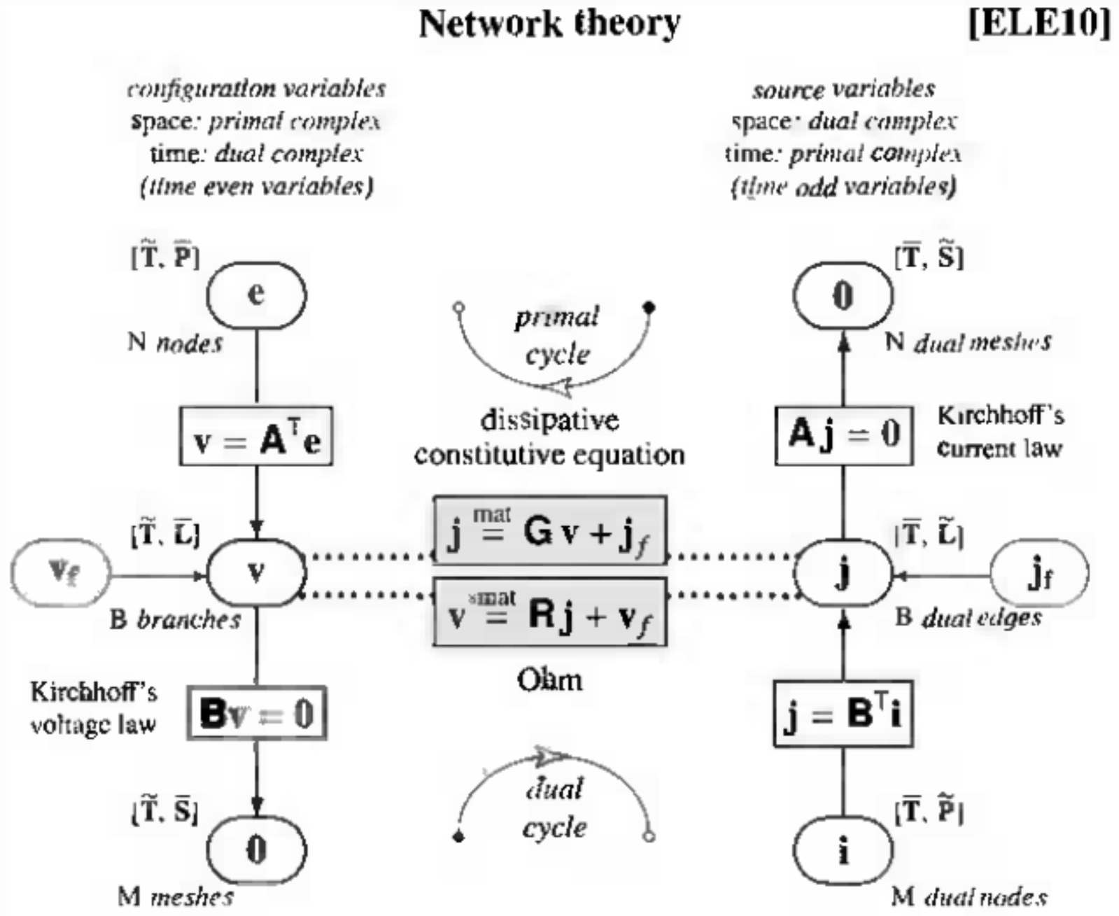
Figure 8: ELE10 (1) in primal complex, assume a 0-cochain of node potential voltages . (2) conduct coboundary operation over to obtain 1-cochain of voltage drops . If 1-cochain voltage sources exist, it will be reduced by to obtain a new 1-cochain of voltage drops .(3) take advantage of dissipative constitutive equation to obtain 1-cochain of branch currents , where is 1- cochain current sources. is now in dual complex (4) conduct boundary operation of , then a null 0-cochain of node currents is obtained because flows at a node sum to zero in conservative field. The process is usually called node potential method. The is obtained as follows:
(12) The second method is based on Kirchhoff’s current law. (1) in dual complex, assume a 2-cochain of mesh currents (2) conduct boundary operation over to obtain 1-cochain of branch currents . If 1-cochian current sources exist, it will be reduced by to obtain a new 1-cochain of branch currents (3) take advantage of the dissipative constitutive equation to obtain 1-cochain of voltage drops . is now in primal complex. (4) conduct boundary operation of , then a null 2-cochain of loop voltage drops is obtained because voltage drops around a loop sum to zero in conservative field. The process is usually called mesh current method. The is obtained as follows:
(13) All the single-domain network problems of pure generalized resistors in steady state can be solved following this semantics. If the network problem includes not only generalized resistors but also generalized capacitors and inductors, multiple time-dependent constitutive equations and time derivatives will be contained. Diagram ELE10 is not sufficient on network problems of mixed generalized resistors,capacitors and inductors.
-
ii.
Typical methods to solve non-ODE equations.
-
iii.
Example:[Fig.9(a)]
(a) An electrical circuit of pure resistances 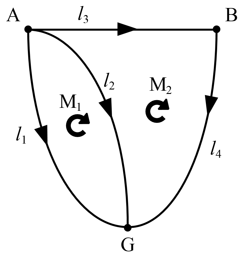
(b) topological structure of R problem Figure 9: A non-ODE electric circuit problem -
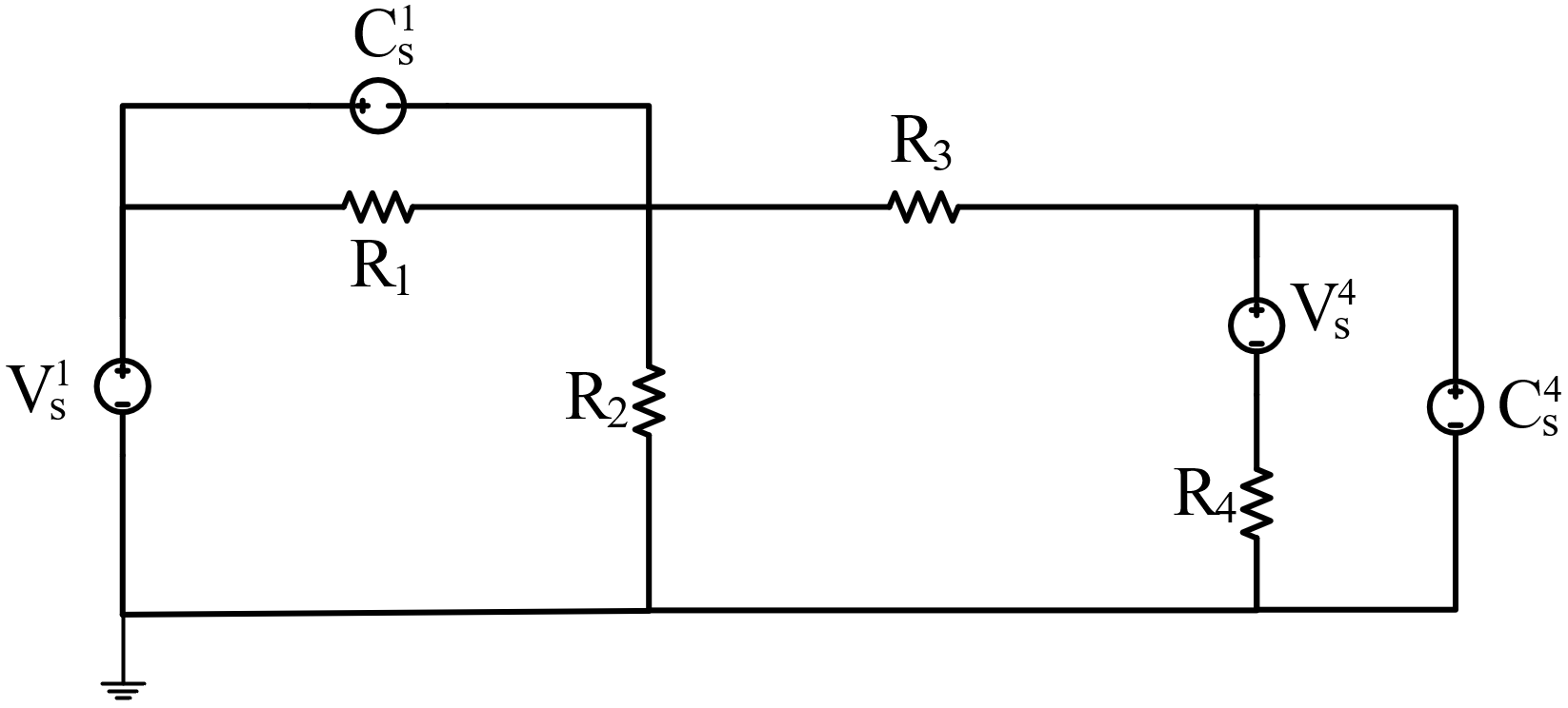
i.
Fig.9(a) shows a electric circuit problem of pure resistance. , are two voltage sources; , are two current sources; are four resistors. The topological structure of this problem is given in Fig.9(b). It is a 2 dimensional cell complex with three 0-cells, four 1-cells and two 2-cells.
If use node potential method to solve this problem, for Fig.9(b),(14) (15) (16) (17) Hence, the 0-cochain node potential voltage can be obtained by Eq.12; Moreover, the 1-cochain branch voltages can be obtained by and the 1-cochain branch currents can be deduced by constitutive equations.
If use node mesh current method to solve this problem,for Fig.9(b),(18) Hence, the 2-cochain mesh current can be obtained by Eq.13; The 1-cochain branch voltages can be obtained by and the 1-cochain branch voltages can be deduced by constitutive equations.
-
(a)
-
4.
System of multiple time-dependent constitutive relations
-
(a)
Time domain method
-
i.
Time included, ODE included, linear
If the constitutive equations of elements include time differential forms, the state equation of system behavior will be an ODE in differential formulations. Typical forms of constitutive equations in physical problems are and , where and are generalized capacitors and inductors. For this part, we will focus on modeling systems consisting of multiple time-dependent constitutive relations. Examples are RLC electrical circuits. Generalized RLC problems in other physical systems can be solved in a similar way
-
ii.
Follow routes in Tonti diagram to obtain state equations. [Fig.10]
To model the RLC electrical circuit problems, we have to resort to three dimensional cell complexes (two dimensional space and one dimensional time) since coboundary of time element is associated to the time derivative in an algebraic way. Combination of [ELE10] and [ELE11] of Tonti diagram provides a model of RLC systems, where two forms of state equations exist that are dual to each other, one of which is shown in [ELE11] of Tonti diagram as follows:
(19) The other dual form is
(20) Because electric charge , the first equation can be written as
(21) Because electric potential impulse , the second equation can be written as
(22) The algebraic form of Eq.21 and Eq.22 can be obtained by following paths in Fig.10.
.png)
(a) Tonti diagram of RLC electric circuit problem .png)
(b) mesh current method .png)
(c) node potential method Figure 10: routes and state equations
In Figure 10(b), each route of different color has its particular physical meaning. Take blue route as an example: we start at 0-cochain of electric potential impulse in primal space and dual time cell complexes. Conduct coboundary operation of to obtain 1-cochain of magnetic flux . Take advantage of constitutive equation to obtain 1-cochain of branch currents . is now in dual space cell complex and primal time cell complex. Conduct boundary operation of , then a null 0-cochain of node currents is obtained because flows at a node sum to zero in conservative field. Other routes can be illustrated in an similar way. If follow the blue, purple and pink route respectively, we obtain three independent items. The diagonal elements in each constitutive matrix represent the behavior in the corresponding vector space. Since it is a linear system, conduct superposition of these three objects. The pure algebraic equation of node potential method is obtained as follows:
(23) where, is 0-cochain of electric potential impulse. is coboundary operation of time in dual complex. is coboundary operation of time in primal complex.
In figure 10(c), analogously, the pure algebraic equation of node potential method is obtained as follows:(24) where, is 2-cochain of mesh current charge.
From Figure 10(b) and 10(c), it is seen that the two methods are dual to each other. -
i.
-
(b)
Example:[Fig.11(a)]
Fig.11(a) shows an RLC electric circuit problem. is resistor; , are capacitors; , are inductors; and are current and voltage sources respectively. Projection of the topological structure of this system (Fig.11(c)) to the two-dimensional cell complex of space are four 0-cells, five 1-cells and two 2-cells as shonw in Fig.11(b).
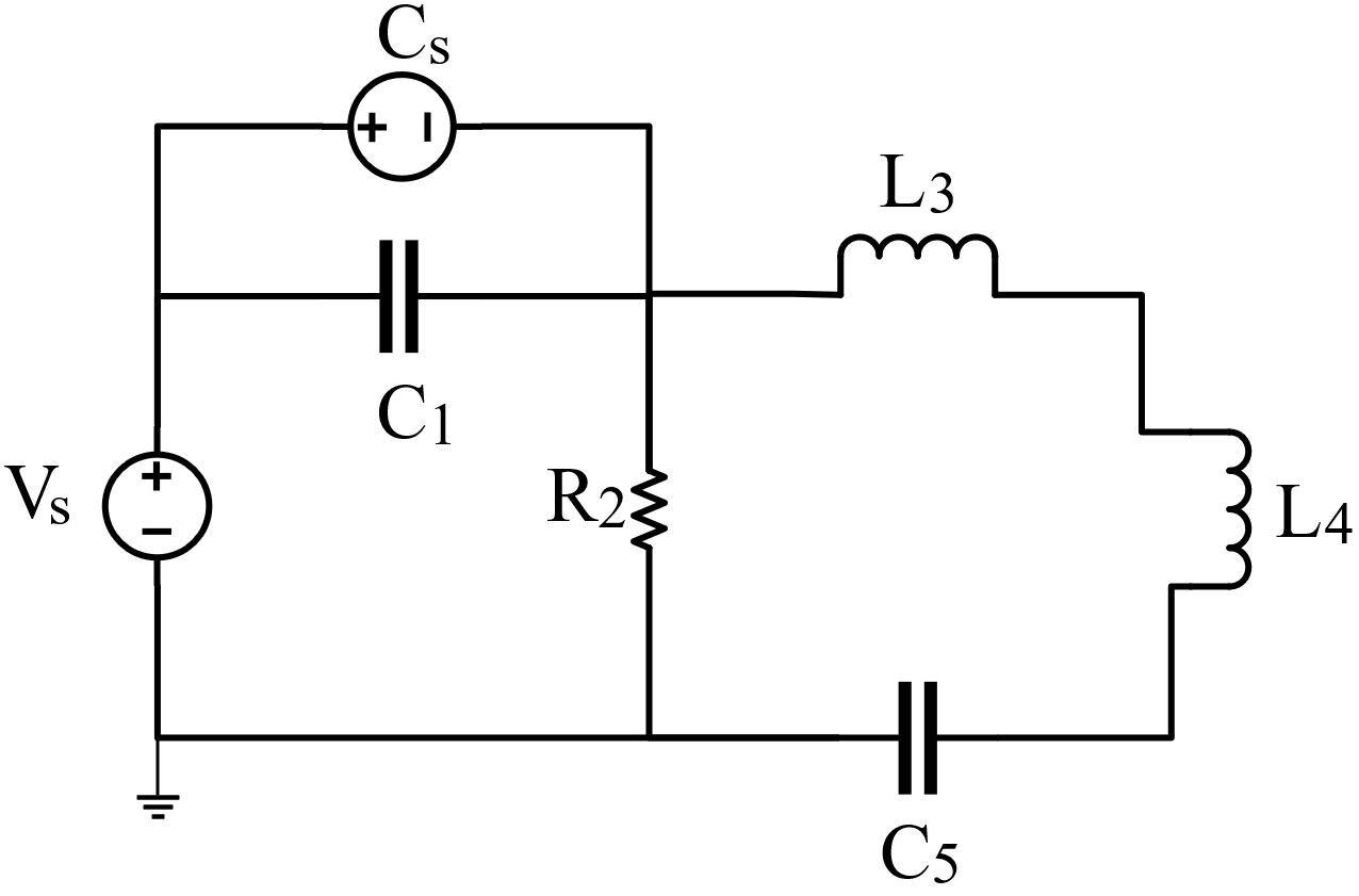
(a) An RLC electrical circuit 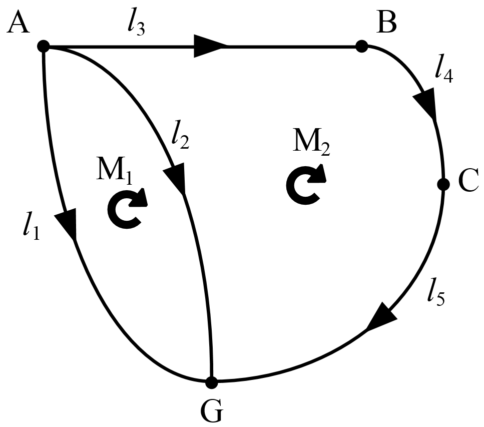
(b) projection of topological structure to space 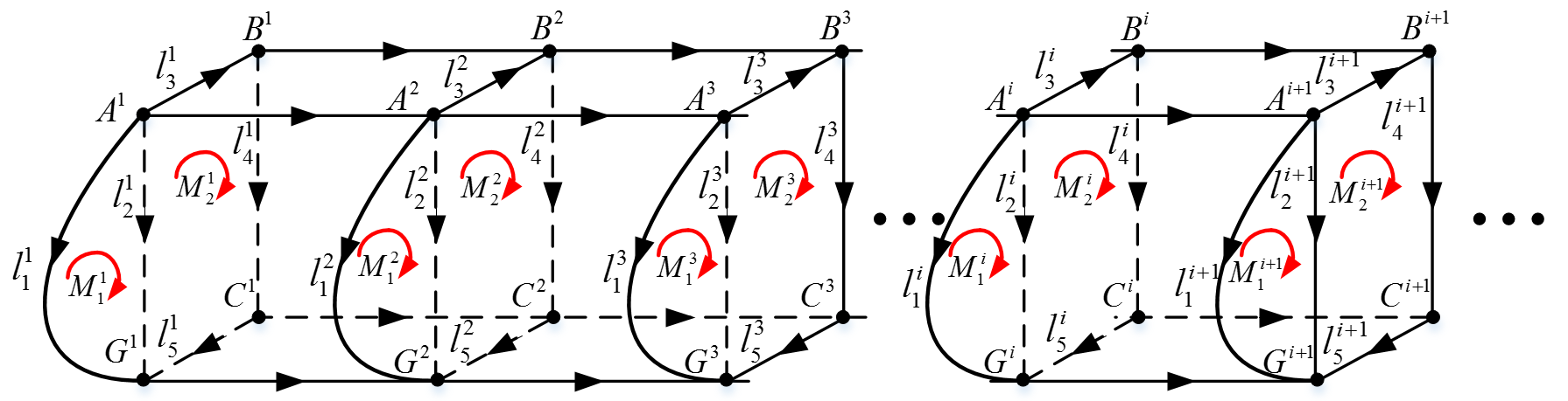
(c) Topological structure of RLC problem Figure 11: An ODE electric circuit problem -
(c)
Laplace frequency domain method
-
i.
Laplace frequency included, pure algebraic equation, linear
Laplace Transform,a linear operator, allows equations in the time domain to be transformed into equivalent equations in the complex s domain. Laplace-domain analysis is the dual of the time-domain analysis. The mathematical definition of the Laplace transform is as follows [poularikas2010transforms]:
(25) The transformation removes from the resulting equation, leaving instead the new variable , a complex number. The Laplace transform converts integral and differential equations into algebraic equations.
The inverse Laplace transform converts a function in the complex -domain to its counterpart in the time-domain. Its mathematical definition is as follows:
(26) Under Laplace transform, integral and differential operators are converted to linear Laplace operators, hence, integral and differential constitutive equations have corresponding algebraic form, which allows the integral and differential variables separate from the integral and differential operators while convert the constitutive variables to its Laplace form satisfying algebraic operation. Since all the constitutive variables can be combined into a single format dependent on s, we call the effect of all constitutive variables impedance.
-
ii.
The typical form of constitutive equations in time domain. i.e. . Linear system means superposition method works.
In Laplace domain, three typical constitutive equations become , and . The physical system in the Laplace domain is still linear since the Laplace operator is linear, thus, the superposition method still works.
-
iii.
Tonti diagram also works in Laplace frequency domain without considering time elements
In Laplace domain, ELE 10 in Tonti diagram is sufficient to model the system of multiple time-dependent constitutive relations. This is because the time derivative items has disappeared, we no longer need time elements, that is to say, only the the diagonal link still remain work, with the extension of constitutive equations associated with it, from only one constitutive equation to a set of constitutive equations , and . Matrices and is now a diagonal matrix of impedance.
-
iv.
Follow routes in Tonti diagram to obtain state equations
The procedure to obtain the state equations (in Laplace domain) is similar to it in terms of system of single constitutive relation.
-
v.
Example:[Fig.11(a)]
As for the example in Fig.11(a), if use node potential method, 0-cochain can be obtained by Eq.12. where,
(27) (28) (29) (30) the 1-cochain branch voltages can be obtained by and the 1-cochain branch currents can be deduced by constitutive equations in Laplace domain.
If use mesh current method, the 2-cochain mesh current can be obtained by Eq.13.where,
(31) The 1-cochain branch voltages can be obtained by and the 1-cochain branch voltages can be deduced by constitutive equations in Laplace domain.
-
i.
-
(a)
-
5.
Signal flows
-
(a)
cell complex model of signal flows [bjorke1995manufacturing]
Examples in Fig.9(a) and Fig.11(a) are both physical interaction models where physical components exchange energy. The energy transmission between components affect both sender and receptor. another type of model is signal flows where the physical components exchange numeric information. The information flow from sender to receptor only affects receptor.
Despite different languages to describe signal flow models, such as signal flow graph, Simulink, Modelilca, etc, they all can be attracted to a directed graph, where nodes are associated with function values and lines represent ordinal scale measurement. Directed graph is a special case of 1-cell complex, hence cell complex can be the tool to model signal flows.
The topological structure of signal flows described by different modeling languages is hidden in the coboundary operator and . represents the incidence of oriented lines (1-cells) and their tails (starting 0-cells); represents the incidence of oriented lines (1-cells) and their heads (ending 0-cells). The coboundary operator is actually the difference . For example, The and of 1-cell complex in Fig.11(b) are as follows:
(32) (33) -
(b)
Example
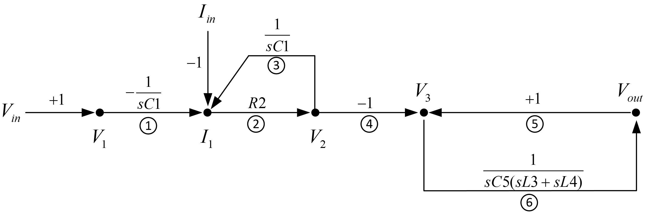
Figure 12: An example of signal flow Fig.12 shows one signal flow model of RLC example ( Laplace domain) in Fig.11(a). The topological structure of it contains five 0-cells and six 1-cells (inputs are not included in the property of topological structure). The local property of the ordinal scale measurement can be described by the Z matrix as follows:
(34) The and representing the connection of 0-cells and 1-cells is as follows:
(35) (36) With Eq.34, Eq.35 and Eq.36, we obtain the global property matrix of the ordinal scale measurement as follows:
(37) Using Eq.37, a set of equations are obtained as follows:
(38) Since there are two loops in the signal flow, the number of state equations are two. If choose , as state variables, state equations can be deduced from Eq. 38 as follows:
(39)
-
(a)
5 Applications - unification
-
1.
Introduction of interoperability
-
(a)
the definition of interoperability [manso2009gis]
-
(b)
Levels of interoperability.
-
i.
Interoperability of algebraic topology (AT) and other modeling languages realizes the semantic interoperability.
-
i.
-
(c)
How can modeling languages below be semantically interpreted in terms of AT model [sjostedt2009modeling]
-
i.
Modelica (Physical-interaction modeling)
Modelica is a multi-domain complex systems modeling language where system models are constructed via block-diagram or command-line user interface.It is an equation-based language building acasual models that permits reuse of classes. Another feature, object-oriented , facilitates this reuse and enhances evolution of models. Using Modelica to modeling, we need to decompose the system to components in a hierarchical top-down way, cite existing classes from appropriate library or self-define new classes for components and define communications between components by existing connectors or self-formulate new interfaces level by level.
For example, when modeling the electrical circuit problem in Fig.11(a) in Modelica, engineers first establish a diagram of this model, then Modelica will turn it into command lines form by automatically extract classes, instances and equations from existing and customer-defined libraries as shown in Fig.14(a), Fig.17 and Fig.15. After that, a ODE/DAE equations system is constructed with two parts, one of which is constitutive equations copied from instants and the other is connection equations derived from intersection between components. Finally, these equations are transformed and simplified to state equations before applying a numerical solver.
Modelica Standard Library gives necessary physical variables and related constitutive equations of individual component as shown in Fig.14(a) and Fig.17. Connection of pins (associated with components) describe the topological structure of the system as shown in Fig.15. These two factors determine Modelica model can be directly interpreted in terms of algebraic topological model. [fritzson2011introduction].
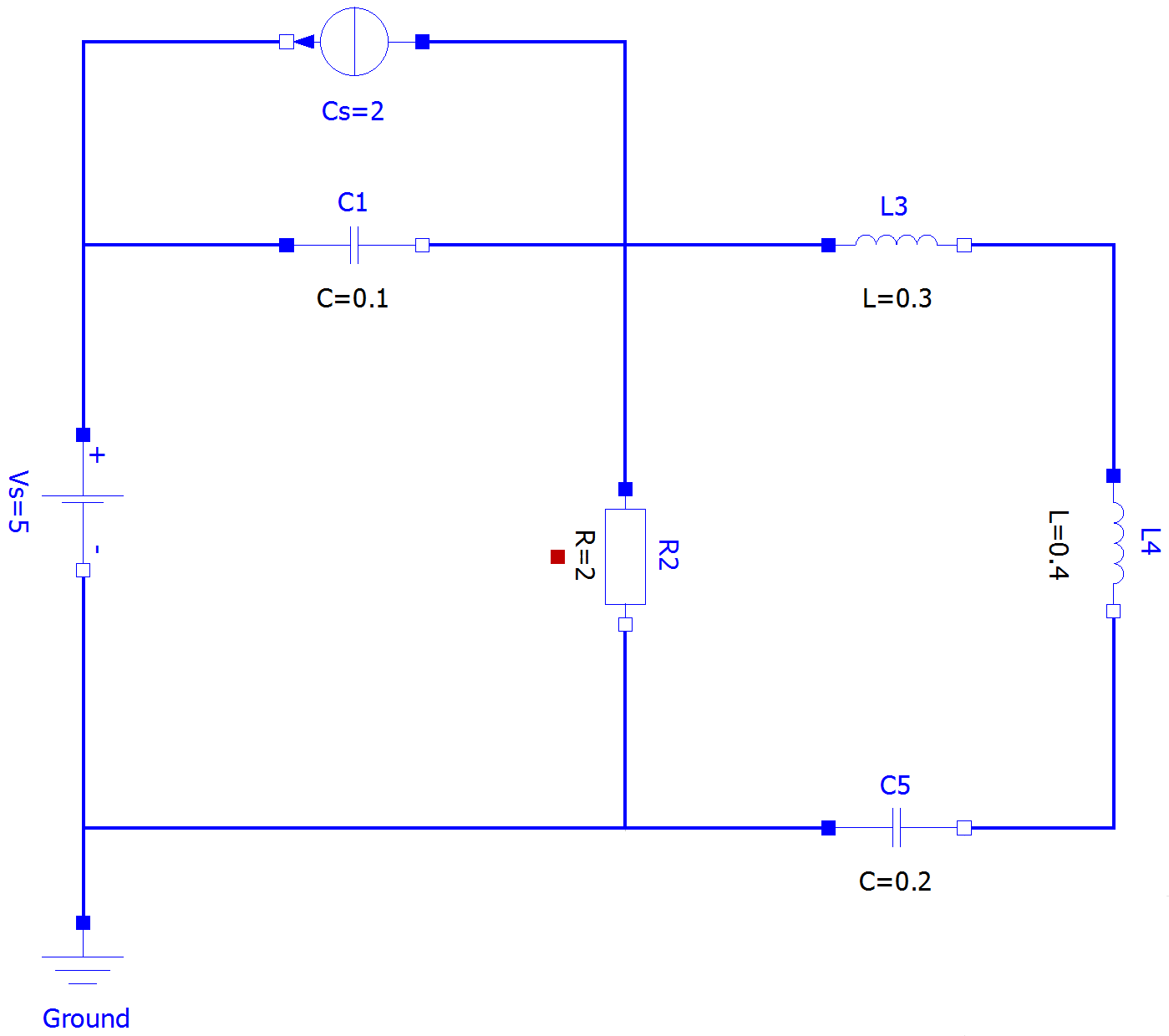
Figure 13: Connection diagram of an electrical circuit model 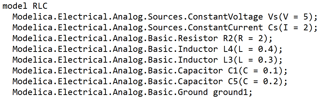
(a) ModelicaRLCcomponents 
(b) ModelicaRLC of R 
(c) ModelicaRLC of L 
(d) ModelicaRLC of C 
(e) ModelicaRLC of Cs 
(f) ModelicaRLC of Vs 
(g) ModelicaRLC of G Figure 14: Equations Extracted from electrical circuit Model an Implicit DAE System 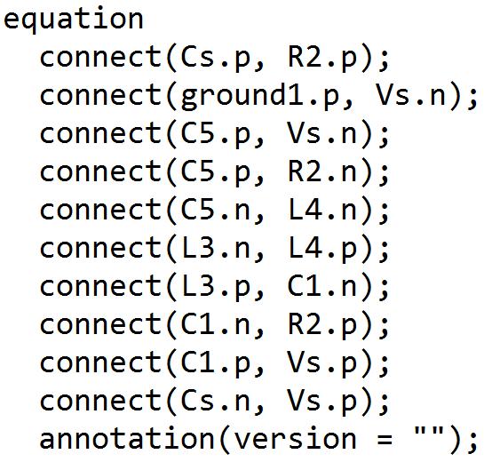
Figure 15: ModelicaRLCconnection -
ii.
Simulink/Simscape (signal-flow modeling) [Fig.16]
-
A.
Variables are associated with ports of blocks. The constitutive equation are given by each block.
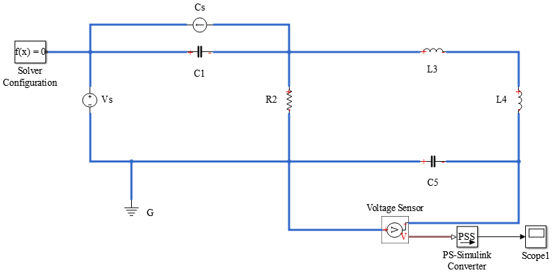
Figure 16: simscape 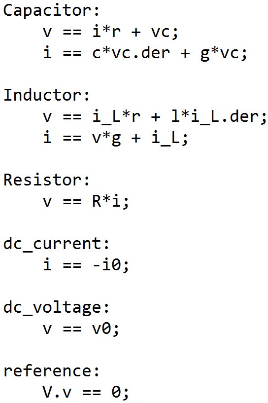
(a) simscapeComponents 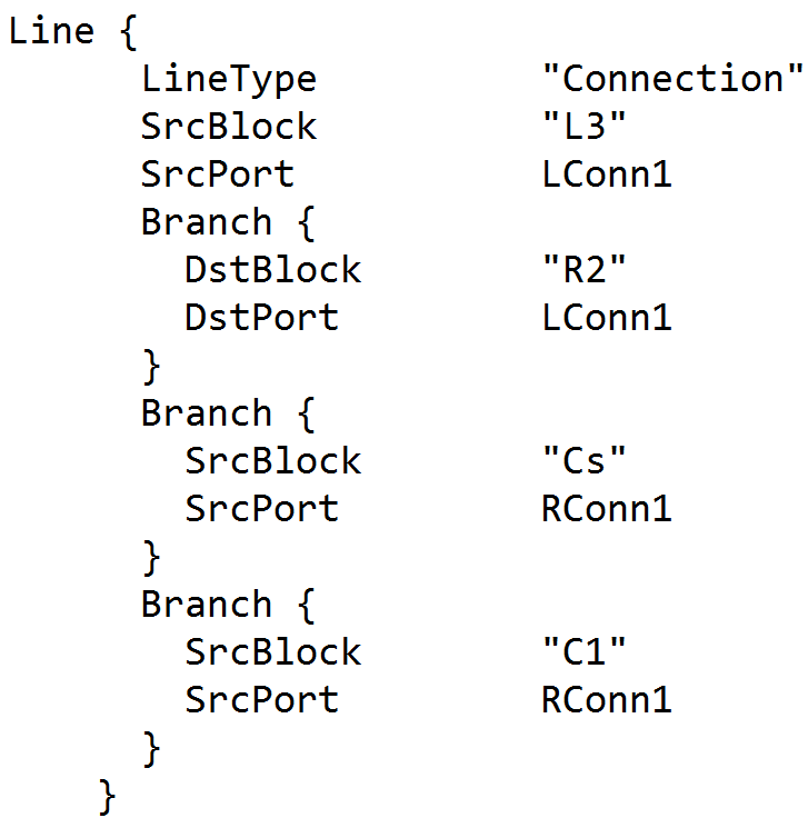
(b) simscapeConnection Figure 17: Equations Extracted -
B.
Links between ports define topological structure of the system
-
A.
-
iii.
Bond graph
Similar to block diagrams, bond graph is a graphical language of a multi-domain physical dynamic system, in which physical energy exchanges bi-directionally on bonds. The usual bond graphs of physical models are the simplest pattern derived from the original schematic diagram of models. All the external bonds include information of physical components and relative constitutive equations. The 0- and 1- junctions in bond graph represent the parallel and serial structure of all physical components of the system, where topological structure hides. For example, Fig.18 shows the bond graph model of electrical circuit problem in Fig.11(a). This model can be read in this way. There are seven components, such as ,, etc. Each component has its corresponding cross, through variables and constitutive equations(usually not drawn in bond graphs). The connection of components can be illustrated as follows. Part 1: and are in a parallel connection, is in serial with them ; Part 2: ,, are in serial connection; Part 3:. Part 1,2 and 3 are parallel. By extracting above information, bond graph model can be directly interpreted in terms of algebraic topological model.
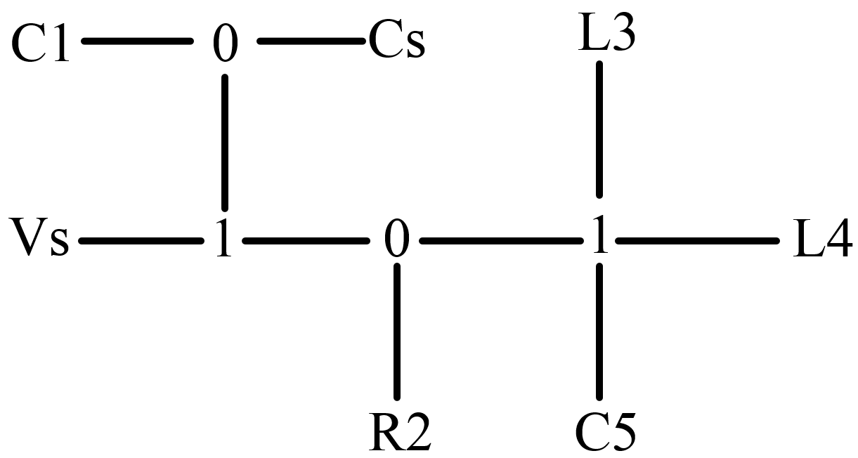
Figure 18: bond graph of RLC problem -
A.
Theoretically speaking, bond graphs can be converted to hypergraphs and hypergraphs include all the topological information required by cell complex.
Given any multiport system described by bond graph, it can be described by a hypernetwork if the bond graph satisfies the following two conditions [gattinger1984hypernetworks]: (1) except for exactly one (non-junction) n-port, every l-junction is bonded to nothing but 0-junctions; (2) every (non-junction) n-port is bonded only to l-junctions. Every bond graph can be converted into an equivalent bond graph satisfying (1) and (2) by inserting 0- and l-junctions if necessary [karnopp2012system]. Conversion to hypernetwork is another way to obtain topological and constitutive information contained in a bond graph and hence provides another method to convert bond graphs to cochain models.
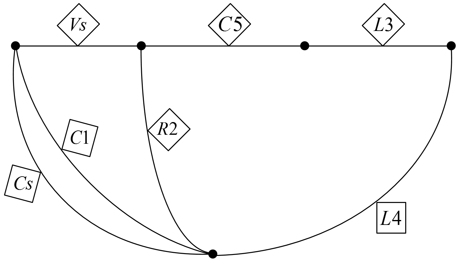
Figure 19: Interpret a bond graph model of an RLC problem as a hypernetwork
-
A.
-
iv.
Linear graph
One of another graphical technique used to form and represent models of dynamic systems is linear graph. Linear graph represent the topological structure of lumped elements connectivity of a system where the branches represent energy port associated with physical components and the nodes represent interconnections of lumped-elements. Because linear graph is a special case of cell complex, all models represented by linear graph can be interpreted directly in terms of algebraic topological model [rowell1997system].
-
A.
linear graph itself is a special case of cell complex.
-
A.
-
v.
NIST model (SysML)
Systems Modeling Language (SysML) is a general-purpose modeling language for engineering systems which is extended for physical interaction and signal flow simulation. SysML takes advantage of internal block diagrams to represent the interconnection of physical components, parametric diagrams and block definition diagrams to construct standard library of physical variables and relative constitutive equations. These three diagrams have all the information required by the algebraic topological model and therefore can be interpreted in terms of algebraic topological model.
-
A.
The variables and constitutive equations of components are defined by parametric diagrams and block definition diagrams [matei2012sysml]
-
B.
The interconnection of pins between blocks in internal block diagrams gives topology of the system
-
A.
-
i.
-
(a)
6 Conclusions and future directions
